1. Introduction
The behaviour of suspended particles in turbulent flows is of considerable interest to a variety of processes, including dispersion of aerosols and collisions of water droplets in the atmosphere, sediment transport and ecological processes in the plankton, see e.g. Shaw (Reference Shaw2003), Balachandar & Eaton (Reference Balachandar and Eaton2010), Guazzelli & Morris (Reference Guazzelli and Morris2011) and Ardekani et al. (Reference Ardekani, Sardina, Brandt, Karp-Boss, Bearon and Variano2017). These applications involve complex interactions between the dispersed and carrier phases, which depend on a large number of parameters: the fluid in which the particles are suspended may be quiescent or turbulent; particles may differ in size, shape, density and stiffness; the dispersed particles can sediment under the action of gravity. The range of temporal and spatial scales involved is wide and the global properties of these suspensions can be substantially different from one case to another. Because of these complexities, our general understanding of the problem is still incomplete (Brandt & Coletti Reference Brandt and Coletti2022).
Solid particles (or droplets) in turbulence are usually categorized by their relative size compared with the smallest turbulent length scale in the dissipative range, the Kolmogorov length scale (Balachandar & Eaton Reference Balachandar and Eaton2010; Dodd & Ferrante Reference Dodd and Ferrante2016). The dynamics of small particles (with the dimension smaller than the Kolmogorov length scale) in homogeneous isotropic turbulence (HIT) has been the object of several earlier studies, see e.g. Squires & Eaton (Reference Squires and Eaton1990), Elghobashi & Truesdell (Reference Elghobashi and Truesdell1993), Boivin, Simonin & Squires (Reference Boivin, Simonin and Squires1998) and Sundaram & Collins (Reference Sundaram and Collins1999). For these particles, the induced turbulence modulation is fully characterized by the ratio of their response time (
 $\tau _p$
) to the Kolmogorov time scale (
 $\tau _{\eta }$
), i.e. the Stokes number
 $St=\tau _p/\tau _{\eta }$
(Ferrante & Elghobashi Reference Ferrante and Elghobashi2003; Yang & Shy Reference Yang and Shy2005). It was found that particles with large Stokes numbers tend to suppress the energy of turbulent eddies of all sizes, whereas the opposite is true for particles whose response time is comparable to the Kolmogorov time scale (
 $St \approx 1$
). For particles with intermediate Stokes numbers between these two limits, however, the energy of the large-scale eddies is attenuated, while the energy of the small-scale ones is enhanced (Poelma & Ooms Reference Poelma and Ooms2006).
When the particle size becomes comparable to or larger than the Kolmogorov length scale (so called finite-size particles), the turbulence modulation cannot be solely predicted by the Stokes number. In this case, changing the particle size or the particle–fluid density ratio has different effects on the turbulence modulation (Lucci, Ferrante & Elghobashi Reference Lucci, Ferrante and Elghobashi2011; Chiarini & Rosti Reference Chiarini and Rosti2024). Finite-size particles usually alter the flow structures comparable or smaller than the particle size (Naso & Prosperetti Reference Naso and Prosperetti2010; Homann, Bec & Grauer Reference Homann, Bec and Grauer2013). For particles of the order of the Kolmogorov length scale, the experiments conducted by Hwang & Eaton (Reference Hwang and Eaton2006) demonstrated the reduced turbulent kinetic energy and dissipation rate when increasing the particle mass loading. Schneiders, Meinke & Schröder (Reference Schneiders, Meinke and Schröder2017) studied decaying turbulence laden with Kolmogorov-scale particles. These authors found that particles absorb energy from the large scales of the carrier phase, whereas the inertial particles increase the local flow dissipation due to the intense strain rate near the particle surfaces. Recently, Chiarini, Tandurella & Rosti (Reference Chiarini, Tandurella and Rosti2025) employed the particle-resolved and point-particle approaches to investigate sub-Kolmogorov particles in sustained turbulence. The comparison between these two different numerical approaches demonstrated that the Eulerian and Lagrangian statistics of the particle phase can be well captured with the point-particle simulation for light particles (particle–fluid density ratio
 $\rho _{\!p}/\rho _{\!f}=5$
). However, for the heavy particles with
 $\rho _{\!p}/\rho _{\!f}\sim 100$
, the discrepancy between the two approaches is non-negligible even in dilute cases, since the particle-induced turbulence modulations at small scales in turn alter the particle dynamics.
As regards larger particles with size of the Taylor length scale, plenty of studies have been performed. Using particle-resolved simulations, Ten Cate et al. (Reference Ten Cate, Derksen, Portela and Van Den Akker2004) showed that the presence of particles attenuates the turbulent kinetic energy at large scales and enhances the dissipation rate in the particle boundary layers. Lucci, Ferrante & Elghobashi (Reference Lucci, Ferrante and Elghobashi2010) numerically investigated the particle-laden decaying turbulence and demonstrated that the increased strain rate in the vicinity of the particle surface enhances the viscous dissipation, an effect becoming more pronounced for particles with higher density. Similarly, Shen et al. (Reference Shen, Peng, Wu, Chong, Lu and Wang2022) and Oka & Goto (Reference Oka and Goto2022) also reported the additional energy dissipation in the wake region surrounding the dispersed particles. This mechanism is intensified with increased particle Reynolds number and is responsible for the observed turbulence attenuation (Shen et al. Reference Shen, Peng, Wu, Chong, Lu and Wang2022). Nevertheless, augmentation of turbulence was also reported due to the vortex shedding of large particles at high particle Reynolds numbers (Gore & Crowe Reference Gore and Crowe1989; Hetsroni Reference Hetsroni1989). More recently, Chiarini & Rosti (Reference Chiarini and Rosti2024) numerically studied the turbulence modulation by finite-size particles of different size at a high Taylor Reynolds number
 ${\textit{Re}}_\lambda =400$
. It was found that particles with different sizes and density ratios have different influences on the energy transfer within the carrier fluid: the fluid–solid interactions become important for heavy particles since the viscous dissipation is amplified even in the regions away from highly inertial particles due to the flow separation. To summarize, the occurrence of both turbulence attenuation and augmentation demonstrates the complicated interactions between the particle and fluid phases of different properties. To predict the turbulence modulation, some empirical criteria that combine different governing factors (e.g. particle size, solid–fluid density ratio, particle volume fraction and the flow Reynolds number) have been proposed based on experimental and numerical data (Tanaka & Eaton Reference Tanaka and Eaton2010; Peng, Sun & Wang Reference Peng, Sun and Wang2023; Balachandar, Peng & Wang Reference Balachandar, Peng and Wang2024).
From a different perspective, the dynamics and spatial distribution of the finite-size particles are also relevant and significantly influenced by the carrier turbulent flow. Homann & Bec (Reference Homann and Bec2010) and Cisse, Homann & Bec (Reference Cisse, Homann and Bec2013) investigated the motion of a single sphere in forced turbulence by means of particle-resolved simulations. These authors found that the particle–fluid slip velocity of neutrally buoyant particles increases with the particle size with a scaling law of
 $(D/\eta )^{2/3}$
. As regards the particle collective behaviour, Fiabane et al. (Reference Fiabane, Zimmermann, Volk, Pinton and Bourgoin2012) experimentally studied the spatial distribution of finite-sized particles in turbulence, and observed the clustering of particles heavier than the fluid, with the neutrally buoyant particles showing no clustering. Accordingly, it was argued that the Stokes number, which is commonly used to characterize the preferential concentration of heavy small particles in turbulence (Squires & Eaton Reference Squires and Eaton1990; Balachandar & Eaton Reference Balachandar and Eaton2010; Monchaux, Bourgoin & Cartellier Reference Monchaux, Bourgoin and Cartellier2012), is not the most appropriate parameter to predict the spatial distribution of finite-size particles. Note that, particle clustering was also reported in the numerical simulations of finite-size particles in turbulence (Jin et al. Reference Jin, Wang, Zhang and He2013; Uhlmann & Chouippe Reference Uhlmann and Chouippe2017; Chiarini & Rosti Reference Chiarini and Rosti2024). The tendency of clustering for particles of Taylor length scale was found to be weakened with increasing particle size (Uhlmann & Chouippe Reference Uhlmann and Chouippe2017). The collective behaviours of the dispersed particles, in particular the particle clustering and relative motions, play a significant role in the particle collision efficiency, a key issue relevant to a variety of natural and industrial applications (Pumir & Wilkinson Reference Pumir and Wilkinson2016).
The problem becomes more complicated when the particle sedimentation is taken into consideration. Without the background turbulent flows, it has been found that settling particles in an initially quiescent fluid can form microstructures with different morphology at varying particle settling Reynolds numbers (Yin & Koch Reference Yin and Koch2007; Uhlmann & Doychev Reference Uhlmann and Doychev2014; Zaidi, Tsuji & Tanaka Reference Zaidi, Tsuji and Tanaka2014). The drafting–kissing–tumbling (DKT)-related hydrodynamic interactions between settling particles are responsible for the formation of particle microclusters that alter the particle settling rate (Uhlmann & Doychev Reference Uhlmann and Doychev2014; Zaidi et al. Reference Zaidi, Tsuji and Tanaka2014). The particle shape also plays a significant role once settling is considered, see e.g. Fornari, Ardekani & Brandt (Reference Fornari, Ardekani and Brandt2018), Moriche et al. (Reference Moriche, Hettmann, García-Villalba and Uhlmann2023) and Jiang, Zhao & Brandt (Reference Jiang, Brandt, Xu and Zhao2025), yet only spherical particles are considered in this study. Recently, Jiang et al. (Reference Jiang, Brandt, Xu and Zhao2025) investigated the pseudoturbulence induced by settling particles. The gravity-driven motion of the particles produces flow fluctuations that are anisotropic along the horizontal and vertical directions, and the particle–fluid interactions are crucial for the energy transfer in the particle-induced pseudoturbulence. When the background turbulence is taken into account, small heavy particles in HIT, typically at volume fraction lower than
 $10^{-4}$
, were reported to settle faster than isolated particles in quiescent flows (Wang & Maxey Reference Wang and Maxey1993; Aliseda et al. Reference Aliseda, Cartellier, Hainaux and Lasheras2002; Petersen, Baker & Coletti Reference Petersen, Baker and Coletti2019). This observation was explained by the so-called ‘preferential sweeping’ effect, i.e. the inertial particles tend to preferentially accumulate in the high-strain regions where downward fluid flows dominate, so the particle settling speed is enhanced (Wang & Maxey Reference Wang and Maxey1993). This effect was found to maximize when the particle relaxation time matches the turbulence viscous time, i.e.
 $St \sim O(1)$
. The settling enhancement is further strengthened when the feedback from the particle to the carrying flow is non-negligible, since the settling particles drag the surrounding fluid downwards, which in turn accelerates the particle settling motions (Bosse, Kleiser & Meiburg Reference Bosse, Kleiser and Meiburg2006; Monchaux & Dejoan Reference Monchaux and Dejoan2017; Huck et al. Reference Huck, Bateson, Volk, Cartellier, Bourgoin and Aliseda2018; Tom, Carbone & Bragg Reference Tom, Carbone and Bragg2022; Bhattacharjee et al. Reference Bhattacharjee, Tom, Carbone and Bragg2024). However, opposite is true for finite-size particles. By virtue of the particle-resolved simulations, the mean settling velocity of particles of
 $D\sim O(10) \eta$
in HIT was found to be lower than that of the isolated particle settling in the quiescent fluid (Chouippe & Uhlmann Reference Chouippe and Uhlmann2015; Fornari et al. Reference Fornari, Picano and Brandt2016a
,
Reference Fornari, Picano, Sardina and Brandtb
, Reference Fornari, Zade, Brandt and Picano2019). The nonlinear and unsteady effects increase the drag acting on settling particles in turbulent flows, so as to reduce the particle settling velocity (Chouippe & Uhlmann Reference Chouippe and Uhlmann2015; Fornari et al. Reference Fornari, Picano, Sardina and Brandt2016b
; Peng et al. Reference Peng, Karzhaubayev, Wang, Chen and Niu2025). Furthermore, the collision rate of the settling particles was found to be reduced in dilute cases, mainly due to the less frequent DKT in the presence of turbulence; conversely, the turbulent transport enhances the relative motion between particles in dense suspensions, leading to an increase in the collision rate compared with that in the quiescent fluid (Fornari et al. Reference Fornari, Zade, Brandt and Picano2019).
Despite the studies reviewed above, the turbulence modulation by finite-size settling particles has not been thoroughly investigated so far. From dimensional analysis, homogeneous turbulence laden with settling finite-size particles is governed by five dimensionless parameters, namely the Taylor-scale Reynolds number
 ${\textit{Re}}_{\lambda }$
, the particle-to-Kolmogorov size ratio
 $D/\eta$
, the particle-to-fluid density ratio
 $\rho _{\!p}/\rho _{\!f}$
, the particle volume fraction
 $\phi$
and the Galileo number
 ${\textit{Ga}}$
, instead of simply the Stokes number and volume and mass loadings as in the point-particle-laden turbulence (Brandt & Coletti Reference Brandt and Coletti2022). The Galileo number
 ${\textit{Ga}}$
here is a dimensionless parameter measuring the buoyancy and viscous force acting on settling particles, see § 2 for the concrete definition. Especially, how the turbulence intensity and the energy transfer in the carrier flow change with the particle settling velocity, which is relevant in many practical applications, yet remains unclear. Therefore, in this study, we aim to explore the effect of sedimentation velocity on the particle-induced turbulence modulation. To this end, we perform particle-resolved direct numerical simulations (PR-DNS) of finite-size particles settling in sustained HIT over a range of Galileo numbers
 ${\textit{Ga}} \in [0,120]$
. Variations in
 ${\textit{Ga}}$
are achieved by changing the particle–fluid density ratio while keeping the particle diameter fixed at the Taylor microscale (i.e.
 $O(10)$
Kolmogorov length scales). In contrast to previous PR-DNS studies of settling particles in HIT, which mostly considered dilute suspensions with
 $\phi \lt 0.5 \,\%$
(Chouippe & Uhlmann Reference Chouippe and Uhlmann2015; Fornari et al. Reference Fornari, Picano, Sardina and Brandt2016b
; Peng et al. Reference Peng, Karzhaubayev, Wang, Chen and Niu2025), we focus on a non-dilute regime at
 $\phi = 10\,\%$
. This choice of volume fraction allows for an appreciable modulation of the background turbulence by the settling particles. In particular, we observe a pronounced reshaping of the energy spectrum, including the emergence of a
 $\kappa ^{-3}$
scaling and marked anisotropy of energy distribution at intermediate scales. A scale-by-scale (SBS) energy budget analysis is conducted to study the underlying mechanisms. Apart from the fluid phase, the particle-phase statistics, including the settling velocity reduction, clustering and collision rate, are also investigated and compared with previous studies.
The remainder of this paper is organized as follows. In § 2, we briefly introduce the numerical method and the analysis tools employed in this study. Then, in § 3, we present the results of the simulations, including the statistics of the fluid flow and particle motion, the energy spectra and energy transfer within the carrier flows, and document the particle clustering and collision rates. Finally, we draw the main conclusion of this work in § 4.
2. Methodology
2.1. Governing equations and numerical methods
In the present study, we use the PR-DNS based on the immersed boundary method (IBM) to simulate the turbulent flow laden with finite-size particles. The fluid flow is governed by the incompressible Navier–Stokes (NS) equations as follows:
 \begin{align} \boldsymbol{\nabla }\boldsymbol{\cdot }\boldsymbol{u} &=0 , \end{align}
 \begin{align} \frac {\partial \boldsymbol{u}}{\partial t}+\boldsymbol{u} \boldsymbol{\cdot }\boldsymbol{\nabla }\boldsymbol{u} &=-\frac {1}{\rho _{\!f}}\boldsymbol{\nabla }\!p+ {\nu } {\nabla} ^{2} \boldsymbol{u}+ \boldsymbol{f}_{\!\textit{ext}}+ \boldsymbol{f}_{\!\textit{ib}} - \langle \boldsymbol{f}_{\!\textit{ib}} \rangle _\varOmega . \end{align}
Here,
 $\boldsymbol{u}=[u_x, u_y, u_z]$
is the fluid velocity vector,
 $p$
is the pressure, and
 $\rho _{\!f}$
and
 $\nu$
denote the density and kinematic viscosity of the Newtonian fluid. In (2.2), the body forcing term
 $\boldsymbol{f}_{\!\textit{ext}}$
represents the external forces that sustain the turbulent flow. Specifically, we employ the method proposed initially by Eswaran & Pope (Reference Eswaran and Pope1988) to compute
 $\boldsymbol{f}_{\!\textit{ext}}$
(denoted as ‘EP’ forces hereinafter). In brief, the body forces are obtained in the physical space from the inverse Fourier transformation of a set of random forces
 $\boldsymbol{\hat {f}}$
defined on
 $\|\boldsymbol{\kappa }\|\leqslant \kappa _{\!f}$
in the spectral space. Here,
 $\kappa _{\!f}$
is the cutoff wavenumber; the random forces are generated in the spectral space with Ornstein–Uhlenbeck processes. The readers are referred to Eswaran & Pope (Reference Eswaran and Pope1988) and Chouippe & Uhlmann (Reference Chouippe and Uhlmann2015) for more details about the computation of
 $\boldsymbol{f}_{\!\textit{ext}}$
.
The other forcing term
 $\boldsymbol{f}_{\!\textit{ib}}$
in (2.2) denotes the immersed-boundary (IB) forcing term for modelling the particle–fluid interactions. In particular, we employ the direct-forcing IBM with multiforcing corrections (Uhlmann Reference Uhlmann2005; Breugem Reference Breugem2012). Note that the spatial average of the IB forcing term,
 $\langle \boldsymbol{f}_{\!\textit{ib}}\rangle _{\varOmega }$
, is subtracted from the momentum (2.2) to retain the zero net flow rate (i.e.
 $\langle \boldsymbol{u}\rangle _{\varOmega } = 0$
) for simulations conducted in a triperiodic computational domain (Höfler & Schwarzer Reference Höfler and Schwarzer2000; Chouippe & Uhlmann Reference Chouippe and Uhlmann2015).
As concerns the numerical algorithm, we employ a projection-based finite difference method to numerically solve the incompressible NS equations (2.1)–(2.2), see the original work by Kim, Baek & Sung (Reference Kim, Baek and Sung2002). Specifically, the second-order central difference is employed for the spatial discretization, while the Crank–Nicolson temporal discretization is used for the diffusion and advection terms, leading to a fully implicit advancement in time. After obtaining the predicted velocity by integrating the diffusion and nonlinear terms, a Poisson equation is solved with the fast Fourier transformation algorithm to impose the divergence-free constraint. These schemes retain the second-order accuracy in both time and space (Kim et al. Reference Kim, Baek and Sung2002). For more details and validations of the present numerical method, the readers are referred to our previous publications (Jiang, Xu & Zhao Reference Jiang, Huang, Xu and Zhao2024a , Reference Jiang, Xu and Zhaob ).
The translational and rotational motions of the dispersed particles are governed by the classic Newton–Euler equations:
 \begin{align} \rho _{\!p} V_{\!p} \frac {\mathrm{d} \boldsymbol{v}}{\mathrm{d} t}&=\boldsymbol{F}_{\!H}+\left (\rho _{\!p}-\rho _{\!f}\right ) \boldsymbol{g} V_{\!p}+\boldsymbol{F}_{\!C}, \end{align}
 \begin{align} I_{\!p}\frac {\mathrm{d} \boldsymbol{\omega }}{\mathrm{d} t}&=\boldsymbol{T}_{\!H}+\boldsymbol{T}_{\!C}. \end{align}
Here,
 $\boldsymbol{v}=[v_x,v_y,v_z]$
and
 $\boldsymbol{\omega }=[\omega _x,\omega _y,\omega _z]$
denote the particle linear and angular velocity, respectively. The symbols
 $\rho _{\!p}$
,
 $V_{\!p}$
and
 $I_{\!p}$
represent the density, volume and moment of inertia of the particle, namely
 $V_{\!p}=\pi D^3/6$
and
 $I_{\!p}=\rho _{\!p}V_{\!p}D^2/10$
for a sphere;
 $\boldsymbol{g}$
is the gravity acceleration. The hydrodynamic force and torque acting on the dispersed particles, denoted by
 $\boldsymbol{F}_{\!H}$
and
 $\boldsymbol{T}_{\!H}$
, are obtained by integrating the IB forces (Breugem Reference Breugem2012; Kempe & Fröhlich Reference Kempe and Fröhlich2012). The contact force and torque
 $\boldsymbol{F}_{\!C}$
and
 $\boldsymbol{T}_{\!C}$
, which account for the particle–particle collisions, are modelled by the soft-sphere collision forces with lubrication correction (Jeffrey Reference Jeffrey1982; Costa et al. Reference Costa, Boersma, Westerweel and Breugem2015).
2.2. Simulation set-ups
The simulation cases and set-ups of the present study are summarized in table 1. Before examining the particle-laden flows, we first run one simulation of the single-phase turbulent flow, denoted by ‘case 0’ in table 1, as a reference case. The parameters related to the EP forces are listed in table 2, including the cutoff wavenumber
 $\kappa _{\!f}$
, the time scale of the Ornstein–Uhlenbeck process
 $T_L$
and the amplitude of the random forces
 $\sigma$
(see more details concerning the definition of these variables in Eswaran & Pope (Reference Eswaran and Pope1988) and Chouippe & Uhlmann (Reference Chouippe and Uhlmann2015)). The statistics of the single-phase turbulence obtained with these EP parameters, including the root-mean-square (r.m.s.) velocity fluctuation
 $u'$
, the mean dissipation rate
 $\epsilon$
, the Kolmogorov length scale
 $\eta =\nu ^{3/4}\epsilon ^{-1/4}$
, the Taylor micro scale
 $\lambda =\sqrt {15\nu u'{^2} \epsilon ^{-1}}$
, the integral length scale
 $L_{\textit{int}}=(3u'{^2/2)}^{3/2}\epsilon ^{-1}$
, the Kolmogorov time scale
 $\tau _\eta =\nu ^{1/2}\epsilon ^{-1/2}$
, the turn-over time scale
 $T_e=u'^2/\epsilon$
and the Taylor Reynolds number
 ${\textit{Re}}_\lambda =u'\lambda /\nu$
, are also provided in table 2. Note that the parameters related to the EP forces are kept constant in the particle-laden cases introduced below.
Simulation set-ups. Here,
 $\rho _{\!p}/\rho _{\!f}$
denotes the density ratio between the particle and fluid;
 ${\textit{Ga}}$
is the Galileo number;
 ${\textit{Re}}_{s0}$
is the Reynolds number defined by the settling velocity
 $V_{s0}$
of an isolated particle;
 $L_i$
(with
 $i=x$
,
 $y$
or
 $z$
) is the length of the computational domain;
 $N_i$
is the number of grid cells along the
 $i$
-direction;
 $N_{\!p}$
is the number of particles in the simulation.

Parameters used to generate the external forces that sustain the turbulent flow and the statistics of the single-phase turbulence (denoted by the subscript ‘0’). Here,
 $\kappa _{x,min}=2\pi /L_x$
is the fundamental wavenumber along the
 $x$
-direction,
 $\epsilon ^*=\sigma ^2 T_L$
is a bundled parameter (see Chouippe & Uhlmann Reference Chouippe and Uhlmann2015) and the time scale
 $\tau _p=D^2/18\nu$
represents the relaxation time of the neutrally buoyant particles.

Given the complexity of the current problem (with five governing parameters as stated in the introduction), the objective of the present study is to shed some light on the effect of the sedimentation velocity on the particle dynamics and turbulence modulation in HIT, while the other properties (i.e. the background turbulence intensity, particle size and particle volume fraction) are kept constant. To this end, we design four simulation cases of particle-laden turbulence with varying Galileo numbers, which is realized by adjusting the particle–fluid density ratio
 $\rho _{\!p}/\rho _{\!f}$
, as shown in table 1. The dimensionless parameter
 ${\textit{Ga}}$
, defined by
 ${\textit{Ga}}=\sqrt {(\rho _{\!p}/\rho _{\!f}-1)gD^3}/\nu$
, measures the ratio between the buoyant and viscous force acting on a settling particle in a viscous fluid. The values of
 ${\textit{Ga}}$
are selected by considering spherical particles with a fixed diameter
 $D=2\, \text{mm}$
settling in a Newtonian fluid with kinematic viscosity
 $\nu =1\times 10^{-6}\,\mathrm{m^2\,s^{-1}}$
, and gravity acceleration
 $\| \boldsymbol{g} \|=9.81\,\mathrm{m\,s^{-2}}$
. The particle size is of the order of the Taylor microscale of the single-phase turbulence with
 $D\approx 0.67\lambda _0 \approx 13.5 \eta _0$
(see table 1), and the particle volume fraction is fixed at
 $\phi =N_{\!p} V_{\!p} / V_{\varOmega }=10\,\%$
(where
 $V_\varOmega = L_x L_y L_z$
is the total volume of the domain). Note that the change of the particle–fluid density ratio is relatively small, with values
 $\rho _{\!p}/\rho _{\!f} \in [1, 1.18]$
, indicating a minimal effect of the particle inertia on the results. The choice of parameters mimics slightly buoyant particles in liquid turbulent environments, which is relevant to realistic applications like the microplastic in the ocean, sediment transport and marine snow. The Taylor Reynolds number is chosen to be computationally affordably high while the particle volume fraction is set sufficiently high to induce appreciable turbulence modulation.
The particle settling Reynolds number
 ${\textit{Re}}_{s0}=V_{s0}D/\nu$
, which is defined by the settling velocity of an isolated particle without turbulence,
 $V_{s0}$
, is solely determined by the Galileo number. Here, we estimate the values of
 ${\textit{Re}}_{s0}$
at different
 ${\textit{Ga}}$
by using the following empirical correlation (Yin & Koch Reference Yin and Koch2007):
 \begin{equation} Ga^2=18{\textit{Re}}_{s0}\left[1+0.1935 {\textit{Re}}_{s0}^{0.6305}\right]\!,\quad \text{for}\quad 20\lt {\textit{Re}}_{s0}\lt 260. \end{equation}
As shown also in table 1, the settling Reynolds number increases with the Galileo number, which also results in an increase of the ratio between the settling velocity and the r.m.s. velocity of the background turbulent flow,
 $V_{s0}/u'_0$
. This is a fundamental parameter that we will use to analyse the turbulence modulation by settling particles.
The grid resolutions are set as
 $D=16\Delta x$
in cases 1–3 and
 $D=24 \Delta x$
in case 4 due to the higher settling Reynolds number. In table 1, we also list the ratio between the Kolmogorov length scale and the grid width for each case to demonstrate the sufficient resolution for solving the background turbulent flow, following the criterion of
 $\kappa _{max} \eta = \pi \eta /\Delta x\geqslant 1.5$
(Pope Reference Pope2000). The simulations are conducted in a triperiodic computational domain with the gravity applied along the negative
 $y$
-direction. To minimize the impact of domain periodicity for the cases with particle sedimentation, we elongate the domain along the vertical direction (i.e.
 $L_y = 2L_x$
) in cases 2–4, following the suggestions in Chouippe & Uhlmann (Reference Chouippe and Uhlmann2015).
2.3. Data analysis: SBS spectral analysis
In § 3.3 we will examine the turbulence modulation by means of the SBS analysis in the spectral space. Here we briefly introduce this approach. By multiplying the Fourier transformation of the momentum (2.2) with the complex conjugate of the velocity vector, we obtain the following energy equation for the fluid flow (Frisch Reference Frisch1995; Crialesi-Esposito et al. Reference Crialesi-Esposito, Rosti, Chibbaro and Brandt2022):
 \begin{equation} \frac {\partial E(\boldsymbol{\kappa },t)}{\partial t} = \mathcal{F}_{\textit{ext}}(\boldsymbol{\kappa },t)+\mathcal{F}_{\textit{ib}}(\boldsymbol{\kappa },t)+{\varPi }(\boldsymbol{\kappa },t)+\mathcal{D}(\boldsymbol{\kappa },t). \end{equation}
The definition and physical interpretation of the terms
 $E(\boldsymbol{\kappa },t)$
,
 $\mathcal{F}_{\textit{ext}}(\boldsymbol{\kappa },t)$
,
 $\mathcal{F}_{\textit{ib}}(\boldsymbol{\kappa },t)$
,
 ${\varPi }(\boldsymbol{\kappa },t)$
and
 $\mathcal{D}(\boldsymbol{\kappa },t)$
are as follows:
-
(i)
 $E(\boldsymbol{\kappa },t)= ( {1}/{2})\widetilde {\boldsymbol{u}}\boldsymbol{\cdot }\widetilde {\boldsymbol{u}}^*$
is the energy spectrum;
-
(ii)
${\varPi } (\boldsymbol{\kappa },t )=-({1}/{2} )({\widetilde {\boldsymbol{u}}}^*\boldsymbol{\cdot }\widetilde {\boldsymbol{G}}+\widetilde {\boldsymbol{u}}\boldsymbol{\cdot }{\widetilde {\boldsymbol{G}}}^* )$
is the spectrum of the energy transfer by the advective transport, with
$\boldsymbol{G}=\boldsymbol{u}\boldsymbol{\cdot }\boldsymbol{\nabla }\boldsymbol{u}$
denoting the nonlinear term of the NS equations; -
(iii)
$\mathcal{D} (\boldsymbol{\kappa },t )=( {1}/{2} )({\widetilde {\boldsymbol{u}}}^* \boldsymbol{\cdot }\widetilde {\boldsymbol{V}}+\widetilde {\boldsymbol{u}} \boldsymbol{\cdot }{\widetilde {\boldsymbol{V}}}^* )$
is the spectrum of the viscous dissipation, with
$\boldsymbol{V}= ( {1}/{\nu }) {\nabla} ^2 \boldsymbol{u}$
denoting the viscous term; -
(iv)
$\mathcal{F}_{\textit{ib}} (\boldsymbol{\kappa },t )=({1}/{2}) (\widetilde {\boldsymbol{f}_{\!\textit{ib}}}\boldsymbol{\cdot }\widetilde {\boldsymbol{u}}^*+\widetilde {\boldsymbol{f}_{\!\textit{ib}}}^* \boldsymbol{\cdot }\widetilde {\boldsymbol{u}} )$
is the spectrum of the work of the IB forcing term, which reflects the particle–fluid interactions; -
(v)
$\mathcal{F}_{\textit{ext}} (\boldsymbol{\kappa },t )=({1}/{2}) (\widetilde {\boldsymbol{f}_{\!\textit{ext}}}\boldsymbol{\cdot }\widetilde {\boldsymbol{u}}^*+\widetilde {\boldsymbol{f}_{\!\textit{ext}}}^* \boldsymbol{\cdot }\widetilde {\boldsymbol{u}} )$
is the spectrum of the energy production by the external EP forces.


Here, the notation
 $\tilde {g}=\tilde {g}(\boldsymbol{\kappa },t)$
indicates the Fourier mode of an arbitrary physical-space variable
 $g(\boldsymbol{x},t)$
, and the superscript ‘*’ denotes the complex conjugate. In practice, the wavenumber vector
 $\boldsymbol{\kappa }=(\kappa _{x},\kappa _{y},\kappa _{z})$
is defined on discrete grid points in the spectral space, i.e.
 $\boldsymbol{\kappa }_{lmn}=(\kappa _{x,l},\kappa _{y,m},\kappa _{z,n})=(l\Delta \kappa _x,m\Delta \kappa _y,n\Delta \kappa _z)$
(with the indices
 $l=-N_x/2+1,\cdots ,N_x/2$
,
 $m=-N_y/2+1,\cdots ,N_y/2$
,
 $n=-N_z/2+1,\cdots ,N_z/2$
and the wavenumber increment
 $\Delta \kappa _i=2\pi /L_i$
). Note that the pressure term (the first term on the right-hand side of (2.2)) vanishes in the energy budget of an incompressible flow (Pope Reference Pope2000), and the subtracted spatially averaged IB forcing term
 $\langle \boldsymbol{f}_{\!\textit{IB}} \rangle _\varOmega$
also has a zero contribution to the energy budget. Moreover, after the flow system reaches the steady state, the different terms on the right-hand side of (2.6) balance each other, with
 $\partial E(\boldsymbol{\kappa },t)/\partial t = 0$
. In what follows, we shall omit the independent variable
 $t$
and express the spectra only as function of the wavenumber; the statistics are computed by the time average at the steady state.
To understand the energy budget on the different scales, the most common approach is to compute the energy as function of the wavenumber magnitude
 $\lvert \boldsymbol{\kappa } \rvert$
by performing an integral over a spherical-shell of radius
 $\lvert \boldsymbol{\kappa } \rvert$
for any arbitrary variable
 $\mathcal{J}(\boldsymbol{\kappa })$
(
 $\mathcal{J}(\boldsymbol{\kappa })$
can stand for
 $E(\boldsymbol{\kappa })$
,
 $\mathcal{F}_{\textit{ext}}(\boldsymbol{\kappa })$
,
 $\mathcal{F}_{\textit{ib}}(\boldsymbol{\kappa })$
or
 $\mathcal{D}(\boldsymbol{\kappa })$
or
 ${\varPi } (\boldsymbol{\kappa })$
), i.e. (Pandey, Ramadugu & Perlekar Reference Pandey, Ramadugu and Perlekar2020)
 \begin{equation} \mathcal{J}(\kappa )=\sum _{\kappa -0.5\Delta \kappa \leqslant \|\boldsymbol{\kappa }'\|\lt \kappa -0.5\Delta \kappa } \mathcal{J}(\boldsymbol{\kappa }'), \end{equation}
where
 $\Delta \kappa =\max \{\Delta \kappa _x,\Delta \kappa _y,\Delta \kappa _z\}$
. However, with the introduction of gravity, the isotropy of the spectra in the spectral space would be broken. Hence, to additionally provide the directional information of an anisotropic spectrum, we adopt as independent variables the horizontal and vertical wavenumbers and define a two-dimensional function of the spectral density (with notation
 $\tilde {\boldsymbol{\cdot }}$
) as
 \begin{equation} \tilde {\mathcal{J}}(\kappa _h,\kappa _y) = \frac {1}{N_{h}(\kappa _h,\kappa _y)}\sum _{\kappa _h-0.5\Delta \kappa _h\leqslant \sqrt {\kappa _x^2+\kappa _z^2}\lt \kappa _h+0.5\Delta \kappa _h}\tilde {\mathcal{J}}(\kappa _x,\kappa _y,\kappa _z). \end{equation}
Here, we compute the average of the spectral density
 $\tilde {\mathcal{J}}(\boldsymbol{\kappa }) = \mathcal{J}(\boldsymbol{\kappa })/(\Delta \kappa _x \Delta \kappa _y \Delta \kappa _z)$
only over the (isotropic) horizontal directions (i.e. on the planes perpendicular to the gravity direction). In the definition (2.8),
 $\kappa _h$
represents the horizontal wavenumber with
 $\Delta \kappa _h=\Delta \kappa _x=\Delta \kappa _z$
, and
 $N_h(\kappa _h,\kappa _y)$
denotes the number of modes satisfying
 $\kappa _h-0.5\Delta \kappa _h\leqslant \sqrt {\kappa _x^2+\kappa _z^2}\lt \kappa _h+0.5\Delta \kappa _h$
for any given
 $\kappa _y$
.
3. Results
3.1. Statistics of the fluid flow
(a) Taylor Reynolds number
 ${\textit{Re}}_\lambda$
versus Galileo number. The black dashed line represents the data of the single-phase turbulence. (b–d) The change of the (b) r.m.s. velocity fluctuations, (c) mean dissipation rate and (d) length scales of the turbulent flow as
 ${\textit{Ga}}$
increases. In panels (b)–(d) the results are normalized by the value of the single-phase turbulence.

We first report the global statistics of the turbulent flows modulated by the dispersed particles, with the results presented in figure 1. First, we can observe from figure 1(a) that the Taylor Reynolds number is smaller for the particle-laden flows than for the single-phase turbulence, and the value of
 ${\textit{Re}}_\lambda$
decreases with
 ${\textit{Ga}}$
. To interpret the change of the Taylor Reynolds number, we compute the velocity fluctuations and the mean dissipation rate of the fluid flow. As shown in figure 1(b), the modulation of the fluid velocity fluctuations by the presence of particles is rather small. The presence of non-settling particles (
 ${\textit{Ga}}=0$
) slightly reduces the r.m.s. of the turbulent flow, indicating the turbulence attenuation. In the cases with non-zero Galileo numbers, the introduction of gravity increases the vertical velocity fluctuation for higher
 ${\textit{Ga}}$
, while the horizontal velocity fluctuation does not change significantly. Consequently, the turbulent flow becomes anisotropic in the suspension of settling particles, an observation that was also reported in the case of a turbulent flow modulated by small settling particles (Bhattacharjee et al. Reference Bhattacharjee, Tom, Carbone and Bragg2024). The greater vertical velocity fluctuation can be ascribed to the conversion of the gravity potential energy to turbulence kinetic energy by the particle settling motions. Without the background turbulence, the fluid flow solely induced by the gravity-driven motion of light bubbles or heavy particles (the so-called pseudoturbulence) is also reported to be anisotropic with larger velocity fluctuations along the direction of gravity (Fornari et al. Reference Fornari, Picano and Brandt2016a
; Amoura et al. Reference Amoura, Besnaci, Risso and Roig2017; Jiang et al. Reference Jiang, Brandt, Xu and Zhao2025). However, the degree of anisotropy is rather low in the present configuration, with the value of
 $u_{y,rms}/u_{x,rms}$
being only 1.09 in the case with the largest settling speed,
 ${\textit{Ga}}=120$
, while it was found to be larger than 2.5 for the particle-induced pseudoturbulence in quiescent fluids (Jiang et al. Reference Jiang, Brandt, Xu and Zhao2025). This is presumably due to the enhanced energy redistribution among the different velocity components by the background turbulent flow.
The particle-induced turbulence modulation is quantified by the ratio of the turbulent kinetic energy of the particle-laden flow and the single-phase flow, denoted by
 $k_{\textit{PL}}/k_{\textit{SP}}$
. Turbulence attenuation is identified when the ratio is less than unity, while
 $k_{\textit{PL}}/k_{\textit{SP}}\gt 1$
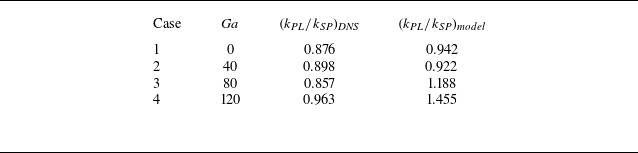
indicates turbulence augmentation (Yu et al. Reference Yu, Xia, Guo and Lin2021). The values of this ratio are presented in table 3 for different cases under study, where we also compare the present simulation results with the theoretical model in Balachandar et al. (Reference Balachandar, Peng and Wang2024). This model predicts the turbulence modulation by the particle phase based on six input parameters: (i) the ratio between the particle size and the Kolmogorov length scale; (ii) the Taylor Reynolds number; (iii) the particle volume fraction; (iv) the mean slip velocity between the particle and fluid phases; (v) the particle-to-fluid density ratio; (vi) the ratio of the viscous dissipation of the particle-laden and single-phase turbulence (see more details in Balachandar et al. (Reference Balachandar, Peng and Wang2024)). As we can see from table 3, this model suggests turbulence attenuation for the cases without or with weak particle sedimentation (cases 1 and 2 with
 ${\textit{Ga}}=0$
and 40), which are in good agreement with the simulation results. However, the model mistakenly predicts turbulence augmentation at
 ${\textit{Ga}}=80$
and 120, when the ratio
 $k_{\textit{PL}}/k_{\textit{SP}}$
remains lower than unity according to the simulation data. This disagreement suggests the need of some model improvement for high-
 ${\textit{Ga}}$
scenarios where significant particle–fluid slip is caused by the relatively fast sedimentation. Note that the model in Balachandar et al. (Reference Balachandar, Peng and Wang2024) was mainly verified against experimental/simulation data without particle settling.
Turbulence modulation by the dispersed particles. The results of the present simulations are denoted by the subscript ‘
 $DNS$
’ and compared with the theoretical model by Balachandar et al. (Reference Balachandar, Peng and Wang2024), indicated by the subscript ‘
 $model$
’.

In contrast to the velocity fluctuations, the mean dissipation rate of the fluid flow increases significantly as
 ${\textit{Ga}}$
grows, see figure 1(c); this increase is more than linear with
 ${\textit{Ga}}$
and is related to the increase of the system energy supply due to the gravitational settling. A similar enhancement of the dissipation rate was also reported in HIT laden with sub-Kolmogorov settling particles. This effect becomes more prominent for highly inertial particles at a relatively high concentration (see Bhattacharjee et al. Reference Bhattacharjee, Tom, Carbone and Bragg2024), but the degree of dissipation enhancement is generally lower in Bhattacharjee et al. (Reference Bhattacharjee, Tom, Carbone and Bragg2024), probably because of the lower volume fraction in the point-particle simulations. Since the Taylor Reynolds number is related to the dissipation rate by
 ${\textit{Re}}_\lambda \propto \epsilon ^{-1/2}$
, the enhancement of the dissipation rate gives rise to the reduction of
 ${\textit{Re}}_\lambda$
with increasing
 ${\textit{Ga}}$
. In the cases with particle sedimentation (
 ${\textit{Ga}}\gt 0$
), the slip velocity between the particle and the local fluid flow results in shear layers in the vicinity of the particle interface, and thus produces the additional viscous dissipation in this region (Lucci et al. Reference Lucci, Ferrante and Elghobashi2010; Fornari et al. Reference Fornari, Picano and Brandt2016a
; Chiarini & Rosti Reference Chiarini and Rosti2024). As the particle settling velocity further increases, the fluid dissipation rate can be considerably enhanced near the separation region of the particle wakes when the particle Reynolds number is greater than
 $O(100)$
(Chiarini & Rosti Reference Chiarini and Rosti2024). Therefore, the mean dissipation rate increases rapidly at
 ${\textit{Ga}}\geqslant 80$
, which finally balances with the additional energy input from the particles’ gravitational energy. Note also that we observe a slight reduction of the viscous dissipation rate compared with the single-phase turbulence in the cases with
 ${\textit{Ga}}=0$
and
 ${\textit{Ga}}=40$
. The particle–fluid slip velocity is rather small in these cases, so the aforementioned mechanism of the wake-related viscous dissipation is negligible. As a matter of fact, in these two cases, the additional particle-induced dissipation (as elaborated in the following section) partially balances the energy input, so as to reduce the fluid viscous dissipation rate.
The enhanced dissipation rate also results in the reduction in the length scales of the turbulence as classically defined for single-phase flows (figure 1
d). As confirmed later by the energy spectra (shown and discussed in § 3.3.1), smaller scales are dynamically active in the presence of particles. We recall here that the Taylor Reynolds number is commonly interpreted as the ratio between the largest and smallest scale in single-phase HIT. From the current data, we observe that, given the same large-scale forcing, the dissipative scale decreases in the presence of particles (see also the energy spectra and spectrum of the viscous dissipation below), which would suggest an increase of
 ${\textit{Re}}_\lambda$
. This is, however, not the case, which indicates that different definitions of these global measures may be required for multiphase flows.
To confirm this first picture of the flow, we provide a visualization of the instantaneous vorticity structures of the fluid flows in cases 0, 1 and 4 in figure 2. Compared with the single-phase turbulence shown in figure 2(a), the presence of non-settling particles (
 ${\textit{Ga}}=0$
case displayed in figure 2
b) slightly reduces the size of the turbulence coherent structures, a difference not obvious in the figure. However, it is easier to observe more fragmented flow structures in the case with non-negligible particle sedimentation (
 ${\textit{Ga}}=120$
, in figure 2
c,d).
Snapshot of the three-dimensional flow field for (a) the single-phase turbulence, (b) the particle-laden flow with
 ${\textit{Ga}}=0$
and (c,d) the case with particle sedimentation at
 ${\textit{Ga}}=120$
. The isosurfaces of the Q criterion (with
 $Q=5u_0'^2/D^2$
in panels (a), (b) and (d), and
 $Q=20u_0'^2/D^2$
in panel (c)) coloured with the
 $y$
-vorticity
 $\varOmega _y$
are used to visualize the vorticity structures in the flow. The dispersed particles (only within the region
 $[L_x/2,L_x]\times [L_y/2,L_y]\times [L_z/2,L_z]$
in panels (b) and (c) are visualized with the black colour. Panel (d) is the zoom-in view of (c) within the box (highlighted by the red cube) of size
 $8D\times 8D\times 8D$
.

3.2. Statistics of particle motions
(a) Time history of the particle-averaged settling velocity. Here,
 $\langle V_s\rangle _p$
is normalized by the respective isolated settling velocity
 $V_{s0}$
for each case (except for the
 ${\textit{Ga}}=0$
case in which the isolated settling velocity of
 ${\textit{Ga}}=40$
is used for normalization since
 $V_{s0}=0$
for zero Galileo number), while time is normalized by the turn-over time scale of the single-phase turbulence,
 $T_{e,0}$
. (b) Closed squares, the ratio between the particle mean settling velocity and the isolated-particle settling velocity; open circles, the hindered settling velocity predicted by the empirical correlation (3.1).

Next, we examine the statistics of the particle motion. The first observation concerns the particle settling velocity in the turbulent flow. In figure 3(a) we present the time history of the particle-averaged (denoted by
 $\langle \boldsymbol{\cdot }\rangle _p$
) velocity of the dispersed particles along the vertical direction, normalized by the settling velocity of an isolated particle in a quiescent fluid,
 $V_{s0}$
. As expected,
 $\langle V_s \rangle _p$
fluctuates around zero at
 ${\textit{Ga}}=0$
, since the particle motion is driven by a turbulent flow with zero mean flow. In contrast, for the cases with non-zero Galileo numbers, the settling velocity of the dispersed particles increases from zero to a steady-state value within an interval of approximately
 $2T_{e,0}$
. After that,
 $\langle V_s \rangle _p$
fluctuates around a constant value so that we can define its time-averaged value as the particle mean settling velocity in suspension, denoted by
 $\langle V_s \rangle$
. The values of
 $\langle V_s \rangle$
are displayed by closed squares in figure 3(b) for the cases under investigation: it is noteworthy that the mean settling velocity in suspensions is smaller than the settling velocity of the isolated particle, regardless of the Galileo number. However, the ratio between
 $\langle V_s \rangle$
and
 $V_{s0}$
is an increasing function of the Galileo number.
Let us elaborate on the reduction of the particle settling speed in the current flow configuration. Firstly, we recall that the hindrance effect, which has been extensively studied for the particle sedimentation in a quiescent fluid, is responsible for the decreased settling velocity in suspensions (Richardson & Zaki Reference Richardson and Zaki1954; Davis & Acrivos Reference Davis and Acrivos1985; Yin & Koch Reference Yin and Koch2007). It was proposed by Richardson & Zaki (Reference Richardson and Zaki1954) that the hindered settling velocity, the average settling velocity in a suspension, decreases with the particle volume fraction, following the empirical correlation
 \begin{equation} \langle V_s \rangle _{\textit{hindered}}/V_{s0} = (1-\phi )^n , \end{equation}
where the exponent
 $n$
can be expressed as a function of the settling Reynolds number
 ${\textit{Re}}_{s0}$
(defined based on the isolated-particle settling velocity
 $V_{s0}$
) (Garside & Al-Dibouni Reference Garside and Al-Dibouni1977):
 \begin{equation} \frac {5.1-n}{n-2.7}=0.1 {\textit{Re}}_{s0}^{0.9}. \end{equation}
We therefore also depict the hindered settling velocities estimated by (3.1) in figure 3(b) with open circles. Interestingly,
 $\langle V_s \rangle _{\textit{hindered}}$
still overestimates the mean settling velocity of the present simulations. There must therefore be a second mechanism active to reduce the particle settling speed: the drag increase related to nonlinear and unsteady drags on the particles in a turbulent environment (Fornari et al. Reference Fornari, Picano, Sardina and Brandt2016b
). These effects play a more significant role when the turbulence fluctuation is stronger than the particle settling velocity, which can be quantified by the ratio
 $u'_0/V_{s0}$
(Fornari et al. Reference Fornari, Picano, Sardina and Brandt2016b
). In other words, the nonlinear and unsteady contributions to the drag decrease in relative value as the settling speed increases in comparison with the turbulence intensity. As a consequence, the difference between
 $\langle V_s \rangle$
and
 $\langle V_s \rangle _{\textit{hindered}}$
is expected to decrease as the ratio
 $V_{s0}/u'_0$
increases (i.e. with the increasing Galileo number), as confirmed by the data shown in figure 3(b).
We further compare the present simulations with previously proposed drag models for settling particles in turbulence. To this end, we define the drag coefficient based on the mean slip velocity between the particle and fluid phases as
 \begin{equation} C_d = \frac {\langle F_d \rangle _p}{\dfrac {1}{2} \rho _{\!f} U_s^2 A}. \end{equation}
Here,
 $\langle F_d \rangle _p$
is the particle-averaged drag force and can be related to the buoyancy as
 $\langle F_d \rangle _p=\pi D^3 (\rho _{\!p}-\rho _{\!f}) g / 6$
;
 $U_s =| \langle V_s \rangle - \langle U_f \rangle |$
is the mean slip velocity;
 $A=\pi D^2 /4$
is the front area of the particle. Note that the fluid phase has a mean upward velocity
 $ \langle U_f \rangle = - \phi \langle V_s \rangle /(1-\phi )$
(the negative sign indicates the opposite direction to the particle mean settling velocity), which maintains the zero net flux of the whole system by compensating the downward flux of the settling particles (Yin & Koch Reference Yin and Koch2007). From the modelling perspective, Xia et al. (Reference Xia, Yu, Pan, Lin and Guo2022) proposed the following correlation for the mean drag coefficient based on their PR-DNS of settling particles in an otherwise quiescent fluid (indicated by the subscript ‘
 $quie$
’):
 \begin{equation} C_{d,\textit{quie}}^{\textit{model}}=\frac {24}{{\textit{Re}}_m}\left(1+0.15{\textit{Re}}_m^{0.687}\right)(1-\phi )^{1-n}, \end{equation}
where the Reynolds number
 ${\textit{Re}}_m$
is defined as
 ${\textit{Re}}_m = (1-\phi ) {\textit{Re}}_p$
with
 ${\textit{Re}}_p = U_s D/\nu$
the particle Reynolds number based on the mean slip velocity, and the index
 $n$
given by the empirical formula
 \begin{equation} n = \left[3.88-0.38 \ln \left({\textit{Re}}_p\right)\right] \ln \left(\phi ^{-1}\right) \left(\rho _{\!p} /\rho _{\!f}\right)^{-0.038}. \end{equation}
Drag coefficient, (
 $\blacksquare$
) present simulation results; (
 $\bullet$
) hindered settling modelled by (3.1); (
 $\blacktriangle$
) the drag model in the otherwise quiescent fluid given by (3.4); (
 $\times$
) the drag model accounting for the background turbulent given by (3.6); (
 $\blacklozenge$
) the turbulence-induced settling attenuation predicted by the model (3.9).

When further accounting for the background turbulent flows, the drag increase can be modelled by multiplying the drag coefficient with the prefactor
 $(1+\psi )$
, i.e. (Xia et al. Reference Xia, Yu, Pan, Lin and Guo2022)
 \begin{equation} C_{d,\textit{turb}}^{\textit{model}}=(1+\psi ) C_{d,\textit{quie}}^{\textit{model}}. \end{equation}
The parameter
 $\psi$
is given by the empirical expression (Xia et al. Reference Xia, Yu, Pan, Lin and Guo2022)
 \begin{equation} \psi = 0.448 \left [\frac {k}{U_s^2}-\left (\frac {k}{U_s^2}\right )_0\right ]^{0.525}, \end{equation}
in which
 $k$
indicates the turbulent kinetic energy;
 $(k/U_s^2)_0$
represents the effect of particle-induced turbulent kinetic energy and can be modelled by (Mehrabadi et al. Reference Mehrabadi, Tenneti, Garg and Subramaniam2015)
 \begin{equation} \left (\frac {k}{U_s^2}\right )_0 = \phi + 1.25 \phi (1-\phi )^3 \exp (-\phi {\textit{Re}}_m^{1/2}). \end{equation}
In addition, another simplified model that predicts the settling velocity of heavy particles in HIT was recently proposed by Peng et al. (Reference Peng, Karzhaubayev, Wang, Chen and Niu2025),
 \begin{align} \frac {V_s^{turb}}{ V_{s0}} = \frac {k_3}{k_3 + {\textit{Re}}_{s0}} \left (\!1+\frac {1}{k_2 + S_L} \right ) + \frac {{\textit{Re}}_{s0} }{k_3 + {\textit{Re}}_{s0}} \left ( \frac {k_1}{k_1+D/\eta _0} \frac {1}{S_L} + \frac {D/\eta _0}{k_1+D/\eta _0} \frac {S_L}{1+S_L}\right )\!, \end{align}
in which
 $V_s^{turb}$
denotes the settling velocity in a turbulent flow,
 $S_L$
represents the ratio between the isolated settling velocity and the r.m.s. velocity of the turbulent flow and
 $k_1$
,
 $k_2$
,
 $k_3$
are fitting parameters that can be simply set to unity (Peng et al. Reference Peng, Karzhaubayev, Wang, Chen and Niu2025). The comparison of the present simulation results with the empirical models introduced above is presented in figure 4. As we can see, ignoring the turbulence effect (hindered settling modelled by (3.1) or (3.4)) leads to an underestimation of the drag coefficient, with the discrepancy reducing with
 ${\textit{Ga}}$
owing to the increase of the ratio between particle settling velocity and the turbulent velocity fluctuations. Nevertheless, the drag coefficient predicted by the (3.4) is superior to the simplified hindrance-settling model given by (3.1). It is surprising that the drag coefficient predicted by the model (3.9) (see the diamonds in figure 4) agrees well with the present simulation results, although the volume fraction effect is not incorporated in this empirical model. Whether this agreement is robust is worthy of further examination since the hindrance effect and the particle-induced turbulence modulation are neglected by this empirical mode, which was mainly assessed at very low volume fractions (Peng et al. Reference Peng, Karzhaubayev, Wang, Chen and Niu2025). Moreover, the model given by (3.6), which accounts for both the hindrance and turbulent effects, overestimates the drag coefficient. This discrepancy may be related to the different flow configuration (vertical channel flows) and different particle properties in the modelling work by Xia et al. (Reference Xia, Yu, Pan, Lin and Guo2022).
Standard deviations of the (a) translational velocity and (b) angular velocity of the dispersed particles.

To gain further insights, we examine the fluctuations of the particle motion. Figure 5 displays the standard deviation of the particle linear and angular velocities along the horizontal and vertical directions. As shown in figure 5(a), the magnitude of the particle velocity fluctuations is of the same order of that of the fluid phase, indicating the dominance of the turbulent transport on the dynamics of the neutrally (or almost neutrally) buoyant particles under consideration. However, it is noteworthy that the standard deviation of the particle vertical velocity decreases when increasing the Galileo number, while the changes of the horizontal velocity fluctuations are hardly visible. Thus, the fluctuations of the particle motions are weaker along the vertical direction than those in the horizontal direction, i.e.
 $\sigma (v_{y})\lt \sigma (v_{x})$
, in agreement with the results by Fornari et al. (Reference Fornari, Picano and Brandt2016a
). This is also in contrast to the fluid phase with a greater velocity fluctuations along the gravity direction (see figure 1
b). Note additionally that the particle velocity fluctuation was found to be higher along the vertical direction for the particle sedimentation in an otherwise quiescent fluid (Fornari et al. Reference Fornari, Picano and Brandt2016a
; Zaidi Reference Zaidi2018; Jiang et al. Reference Jiang, Zhao and Brandt2026).
The larger vertical velocity fluctuations for settling particles in a quiescent fluid were ascribed to the wake-induced hydrodynamic interactions between settling particles. However, with the background turbulence, the turbulent fluctuations disrupt the particle wakes; the particle velocity fluctuations are instead caused mainly by the turbulent eddies in this scenario (Fornari et al. Reference Fornari, Picano and Brandt2016a ). We therefore suggest that the particle settling acts as a filter of the turbulent eddies and thus partially screens the particle motion from the background turbulence. As a consequence, the vertical velocity fluctuations of the dispersed particles decrease with the Galileo numbers. As regards the rotational motion, we observe in figure 5(b) that the standard deviation of the angular velocity around the horizontal direction is higher than that around the vertical direction. This observation, in agreement with the case of particle sedimentation in a quiescent fluid (Jiang et al. Reference Jiang, Zhao and Brandt2026), is explained by the dominant horizontal vorticity in the wakes produced by the settling particles.
3.3. Energy spectra and SBS analysis
In this section, we investigate the turbulence modulation by the presence of dispersed particles in the spectral space. We will first examine the spherical-shell integral of the energy spectra and the corresponding SBS energy budget. Then, we will display the two-dimensional distribution of the spectra in the Fourier space and discuss the anisotropy of the energy budget caused by the particle sedimentation.
3.3.1. The spherical-shell spectral analysis
Spherical-shell energy spectra for single-phase flow (black), particle-laden flows at
 ${\textit{Ga}}=0$
(cyan),
 ${\textit{Ga}}=40$
(red),
 ${\textit{Ga}}=80$
(green) and
 ${\textit{Ga}}=120$
(blue). The energy spectra are normalized by the total kinetic energy
 $E_k = \sum_{\kappa = 0}^{{\kappa _{\textit{max}}}}E(\kappa )$
. The vertical dashed and dotted lines depict the cutoff wavenumber
 $\kappa _{\!f}$
and the wavenumber corresponding to the particle scale,
 $\kappa _d=2\pi /D$
, respectively.

We start with the energy spectrum of the fluid flow. In figure 6 we present the energy spectra of the single-phase and particle-laden turbulent flows as functions of the spherical-shell wavenumber
 $\kappa = \|\boldsymbol{\kappa }\|$
. As we can see, in comparison with the single-phase flow, the energy spectra rise at small scales whereas the energy contained in the large scales is attenuated in the particle-laden turbulent flows, an observation also made in earlier studies on particle-laden turbulence (Wang et al. Reference Wang, Ayala, Gao, Andersen and Mathews2014; Bhattacharjee et al. Reference Bhattacharjee, Tom, Carbone and Bragg2024). This phenomenon of energy depletion at large scales and reinjection into small scales has been attributed to two main mechanisms (Peng et al. Reference Peng, Sun and Wang2023): (i) the promotion of energy transfer by particles due to the enhanced dissipation rate in the vicinity of the particle surfaces (Tanaka & Eaton Reference Tanaka and Eaton2010; Botto & Prosperetti Reference Botto and Prosperetti2012); (ii) the enhanced vorticity stretching caused by the particles (Peng et al. Reference Peng, Sun and Wang2023). As a consequence of the particle-induced energy transfer, a
 $\kappa ^{-3}$
scaling of the energy spectra is observed in the particle-laden flows, an observation widely reported in the case of bubble/particle-induced pseudoturbulence (Lance & Bataille Reference Lance and Bataille1991; Martínez Mercado et al. Reference Martínez Mercado, Chehata Gómez, Van Gils, Sun and Lohse2010; Pandey et al. Reference Pandey, Ramadugu and Perlekar2020; Innocenti et al. Reference Innocenti, Jaccod, Popinet and Chibbaro2021; Jiang et al. Reference Jiang, Brandt, Xu and Zhao2025).
Moreover, we also notice from figure 6 that the pivot wavenumber
 $\kappa ^\bigstar$
, the intersection point of the energy spectra of the single-phase and particle-laden flows, is close to the particle scale (
 $\kappa ^\bigstar \approx \kappa _d$
) for the case without or with weak particle sedimentation velocity (at
 ${\textit{Ga}}=0$
or 40), a similar observation also reported in previous studies of particle-laden turbulent flows (Wang et al. Reference Wang, Ayala, Gao, Andersen and Mathews2014; Peng et al. Reference Peng, Sun and Wang2023; Chiarini & Rosti Reference Chiarini and Rosti2024). However, it is noteworthy that the pivot wavenumber
 $\kappa ^\bigstar$
shifts towards lower wavenumbers with the increase of the Galileo number, indicating an enhanced particle-induced turbulence modulation as the particle sedimentation becomes faster. Accordingly, the
 $\kappa ^{-5/3}$
scaling of the energy spectrum, which characterizes the classic energy cascade in the inertial range of the single-phase turbulent flow, becomes hardly visible in the suspensions with
 ${\textit{Ga}}=80$
and 120. Note that a Kolmogorov scaling
 $\kappa ^{-5/3}$
of the energy of bubble-induced turbulence was identified at the sub-bubble scales in the recent experimental work by Ma et al. (Reference Ma, Tan, Ni, Hessenkemper and Bragg2025) (these authors report the equivalent
 $r^{2/3}$
scaling of the second-order structure function, with
 $r$
being the separation distance) at the high Galileo number of
 ${\textit{Ga}} \sim O(1000)$
. We, however, did not observe such a Kolmogorov scaling at small scales in the present study, probably due to the fact that the Galileo number under consideration is not high enough. Whether a similar scaling can be observed in the settling-particle pseudoturbulence is worth future explorations by experiments/simulations of particle-laden flows at high
 ${\textit{Ga}}$
. We also note that the recent numerical work by Chiarini et al. (Reference Chiarini, Tandurella and Rosti2025) reported a
 $\kappa ^{-4}$
scaling of the energy spectra for the HIT laden with (non-settling) Kolmogorov-size particles. The turbulence modulation by such small particles with gravity sedimentation also needs further examination.
Cumulative SBS energy budget for (a) case 1 with
 ${\textit{Ga}}=0$
and (b) case 4 with
 ${\textit{Ga}}=120$
. The total viscous dissipation
 $\mathcal{D}^\varSigma _{\textit{tot}}=-\sum _{\kappa = 0}^{{\kappa _{\textit{max}}}} {\mathcal{D}( \kappa )}$
is used to normalize the data.

We now examine the SBS energy budget of the fluid flow in each suspension. We first compare in figure 7 the cumulative spherical-shell SBS energy budget for the flow with no particle settling and with the highest Galileo number under study. The cumulative contribution to the budget, denoted by
 $\mathcal{J}^\varSigma (\kappa )$
, is defined as the sum of the spherical-shell spectrum up to the given wavenumber
 $\kappa$
, i.e.
 \begin{align} \mathcal{J}^\varSigma (\kappa )=\sum \limits _{\kappa = 0}^{{\kappa _{\textit{max}}}} \mathcal{J}\left ( \kappa \right ). \end{align}
As shown in figure 7(a), the external EP forces inject energy into the flow system at the scales larger than that of the cutoff wavenumber
 $\kappa _{\!f}$
, effectively serving as an energy source; on the other hand, the energy is dissipated by the viscous stresses. The nonlinear interactions transfer energy from large to small scales with zero net energy production/dissipation in the flow (Pope Reference Pope2000), i.e.
 ${\varPi }^\varSigma =$
0 at the highest wavenumber.
It is noteworthy that the contribution from the IB forces plays a similar role of transferring energy from large to small scales (indicated by the negative slope of
 ${\varPi }^\varSigma (\kappa )$
at low wavenumbers and positive slope at high wavenumbers). However, its contribution to the interscale energy transfer is less important than that of the nonlinear effect at small
 $\kappa$
, while it directly balances dissipation at large
 $\kappa$
. Note additionally that the particle–fluid interactions have a net contribution of energy dissipation (indicated by the negative value of
 $\mathcal{F}_{\textit{ib}}^\varSigma$
at the highest wavenumber
 $\kappa _{max}$
) in the case with
 ${\textit{Ga}}=0$
, a fact which deserves an explanation.
Let us therefore discuss the non-zero energy dissipation due to the particle–fluid interactions. To this end, we resort to the budget of the total fluid kinetic energy
 $E_k=(u_x^2+u_y^2+u_z^2)/2$
in the physical space (see also Chouippe & Uhlmann Reference Chouippe and Uhlmann2015):
 \begin{equation} \frac {{d}}{{\mathrm{d}t}}{\left \langle {{E_k}} \right \rangle _\varOmega } = - {\langle \epsilon \rangle _\varOmega } + {\left \langle {{{\boldsymbol{f}}_{\!\textit{ext}}} \boldsymbol{\cdot }{\boldsymbol{u}}} \right \rangle _\varOmega } + {\left \langle {{{\boldsymbol{f}}_{\!\textit{ib}}} \boldsymbol{\cdot }{\boldsymbol{u}}} \right \rangle _\varOmega }. \end{equation}
Here,
 $\langle \boldsymbol{\cdot }\rangle _\varOmega$
represents the spatial average. The terms on the right-hand side of (3.11) represent the viscous dissipation (
 $- {\langle \epsilon \rangle _\varOmega }$
), the energy input by external forces (denoted by
 $\varPsi _{\textit{ext}}=\left \langle {{{\boldsymbol{f}}_{\!\textit{ext}}} \boldsymbol{\cdot }{\boldsymbol{u}}} \right \rangle _\varOmega$
) and the contribution from the particle–fluid interactions (denoted by
 $\varPsi _{p}=\left \langle {{{\boldsymbol{f}}_{\!\textit{ib}}} \boldsymbol{\cdot }{\boldsymbol{u}}} \right \rangle _\varOmega$
). These terms are related to the energy budget terms in the spectral space by
 \begin{align} \langle \epsilon \rangle _\varOmega =-\sum \limits _{\boldsymbol{\kappa }} \mathcal{D}(\boldsymbol{\kappa }),\quad \varPsi _{\textit{ext}}=\left \langle {{\boldsymbol{f}}_{\!\textit{ext}}} \boldsymbol{\cdot }{\boldsymbol{u}} \right \rangle _\varOmega = \sum \limits _{\boldsymbol{\kappa }} \mathcal{F}_{\textit{ext}}(\boldsymbol{\kappa }),\quad \varPsi _{p}=\left \langle {{\boldsymbol{f}}_{\!\textit{ib}}} \boldsymbol{\cdot }{\boldsymbol{u}} \right \rangle _\varOmega =\sum \limits _{\boldsymbol{\kappa }} \mathcal{F}_{\textit{ib}}(\boldsymbol{\kappa }). \end{align}
Considering the particle energy budget, the term
 $\varPsi _p$
can be related to the particle motions as follows:
 \begin{equation} \begin{aligned} {\varPsi _p} & \approx \underbrace { - \frac {\phi }{{\rho _{\!p}}{V_{\!p}}} \left ( {\frac {{{\rho _{\!p}}}}{{{\rho _{\!f}}}} - 1} \!\right )\!\left [ {{ \rho _{\!p}V_{\!p} \frac {{d}}{{\textrm {d}t}}{{\left \langle {\frac {1}{2}{\boldsymbol{v}} \boldsymbol{\cdot }{\boldsymbol{v}}} \right \rangle }_p}} + {I_{\!p}}\frac {{d}}{{\mathrm{d}t}}{\left \langle {\frac {1}{2}{{\boldsymbol{\omega }}} \boldsymbol{\cdot }{{\boldsymbol{\omega }}}} \right \rangle _p}} \right ]}_{\varPsi _p^{acc}} + \underbrace {\phi \left ( {\frac {{{\rho _{\!p}}}}{{{\rho _{\!f}}}} - 1} \right ){{\left \langle {\boldsymbol{v}} \right \rangle }_p} \boldsymbol{\cdot }{\boldsymbol{g}}}_{\varPsi _p^{\textit{gra}}} \\ &\quad + \underbrace {\frac {\phi }{{{\rho _{\!f}}{V_{\!p}}}}\left [ {{{\left \langle {{\boldsymbol{v}} \boldsymbol{\cdot }{{\boldsymbol{F}}_{\!C}}} \right \rangle }_p} + {{\left \langle {{\boldsymbol{\omega }} \boldsymbol{\cdot }{{\boldsymbol{T}}_C}} \right \rangle }_p}} \right ]}_{\varPsi _p^{col}} \underbrace { - \frac {\phi }{{{V_{\!p}}}}{{\left \langle {{\boldsymbol{v}} \boldsymbol{\cdot }\int _{{\varOmega _p}} {{{\boldsymbol{f}}_{\!\textit{ext}}}{\rm d}V} + {\boldsymbol{\omega }} \boldsymbol{\cdot }\int _{{\varOmega _p}} {{\boldsymbol{r}} \times {{\boldsymbol{f}}_{\!\textit{ext}}}{\rm d}V} } \right \rangle }_p}}_{\varPsi _p^{\textit{ext}}}. \end{aligned} \end{equation}
The derivation of the above equation, which was originally performed in Chouippe & Uhlmann (Reference Chouippe and Uhlmann2015), is provided in Appendix A for completeness. According to (3.13), the total work related to the particle–fluid interactions
 $\varPsi _p$
is composed of the contributions from the particle acceleration
 $\varPsi _p^{acc}$
, the particle sedimentation
 $\varPsi _p^{\textit{gra}}$
, interparticle collisions
 $\varPsi _p^{col}$
and the term related to the external forces
 $\varPsi _p^{\textit{ext}}$
. Note that the term inside the square bracket of
 $\varPsi _p^{acc}$
can be reformulated as
 \begin{align} {{ \rho _{\!p}V_{\!p} \frac { {d}}{{\textrm {d}t}}{{\left \langle {\frac {1}{2}{\boldsymbol{v}} \boldsymbol{\cdot }{\boldsymbol{v}}} \right \rangle }_p}} + {I_{\!p}}\frac {{d}}{{\mathrm{d}t}}{\left \langle {\frac {1}{2}{{\boldsymbol{\omega }}_p} \boldsymbol{\cdot }{{\boldsymbol{\omega }}_p}} \right \rangle _p}} = \frac {1}{2}\frac {{d}}{{\textrm {d}t}}{\left \langle {{\rho _{\!p}}{V_{\!p}}{{\boldsymbol{v}}^2} + {I_{\!p}}{{\boldsymbol{\omega }}^2}} \right \rangle _p}, \end{align}
namely the time derivative of the particle-averaged kinetic energy. Hence,
 $\varPsi _p^{acc}$
can only have a non-zero contribution to the energy budget for a non-equilibrium flow; for example, it works either as a energy source or sink, depending on the particle size, in particle-laden decaying turbulence (Lucci et al. Reference Lucci, Ferrante and Elghobashi2010). In the steady state of sustained turbulence, however,
 $\varPsi _p^{acc}$
is equal to zero. Additionally,
 $\varPsi _p^{\textit{gra}}$
is equal to zero when the particles do not settle (
 ${\textit{Ga}}=0$
). As regards the other two terms in (3.13), the contribution from particle–particle collisions was reported to be negligible at the volume fraction
 $\phi \sim O(0.1)$
(Chiarini & Rosti Reference Chiarini and Rosti2024), which is also confirmed in the present simulations. Hence, from our simulation results, the last term
 $\varPsi _p^{\textit{ext}}$
is mainly responsible for the negative value of
 $\varPsi _p$
in the case of
 ${\textit{Ga}}=0$
, corresponding to a weak but non-negligible net energy dissipation associated with the particle–fluid interactions (see figure 7
a).
As shown in Appendix B, the net dissipation originated from the IB forces at
 ${\textit{Ga}}=0$
is related to the non-zero EP external forces applied also inside the rigid particles. However, as shown in the same appendix, this contribution becomes almost negligible when the external forcing is excluded from the solid region; then the residual contribution is merely from interparticle collisions (
 $\varPsi _p^{col}$
). Note, also, from the definition of
 $\varPsi _p^{\textit{ext}}$
that a negative value of this term indicates a positive correlation between the particle velocities and the external forces sustaining the turbulence, which is attributed to the tendency of neutrally buoyant particles to follow local fluid flows produced by the external forces. Although it might have been preferable to force the turbulence only in the fluid phase, we show that this does not change the physics discussed in this work, especially above the wavenumbers of the external forcing, which acts at the large scale of the computational domain.
Now let us move back to the discussion on figure 7(b), which provides the cumulative SBS budget of the fluid kinetic energy in the suspension with
 ${\textit{Ga}}=120$
. Compared with the non-sedimentation case (
 ${\textit{Ga}}=0$
in figure 7
a), it is obvious that the total work done by the IB forces is significantly augmented. The positive value of
 $\mathcal{F}_{\textit{ib}}^\varSigma (\kappa _{max})$
indicates a net energy input by the particle–fluid interactions at
 ${\textit{Ga}}=120$
. This is because the contribution from the particle sedimentation, i.e.
 $\varPsi _p^{\textit{gra}}$
in (3.13), does positive work in the flow system, which overwhelms the energy dissipation caused by collisions and external forces inside the particles (negative values of
 $\varPsi _p^{col}$
and
 $\varPsi _p^{\textit{ext}}$
); the work done by the settling particles, instead of the energy production by the external EP forces, serves as the major source of the energy input. As a consequence, to close the energy budget, the viscous dissipation becomes greater than
 $\varPsi _{\textit{ext}}$
, different from the physics in the single-phase turbulence.
To have a clearer comparison between different cases, we show the cumulative contributions to the energy budget in figure 8: in particular, we display the nonlinear transfer
 ${\varPi }^\varSigma$
, viscous dissipation
 $\mathcal{D}^\varSigma$
and the particle–fluid interactions
 $\mathcal{F}_{\textit{ib}}^\varSigma$
at different
 ${\textit{Ga}}$
. These comparisons illustrate the modulation of the energy budget in the particle-laden turbulence with varying particle settling velocity. We first observe from figure 8(a) that the total energy input by the IB forces, i.e. the value of
 $\mathcal{F}_{\textit{ib}}^\varSigma$
at the highest wavenumber, increases monotonically with the Galileo number. This enables us to provide an estimate of the ratio between the energy input by the gravity sedimentation and the external forces that sustain the single-phase turbulence:
 \begin{equation} \varLambda = \frac {{{\varPsi _p^{\textit{gra}}}}}{{{\varPsi _{\textit{ext}}}}} \approx \frac {{{\varPsi _p^{\textit{gra}}}}}{{{\epsilon _0}}} = \frac {{\phi \left ( {{\rho _{\!p}}/{\rho _{\!f}} - 1} \right )g\left \langle {{V_s}} \right \rangle }}{{{\epsilon _0}}} = \frac {{\phi G{a^2}{{\textit{Re}}_s}}}{{5832\epsilon _0^*}}. \end{equation}
Here,
 ${\textit{Re}}_s=\langle V_s \rangle D/\nu$
is the Reynolds number based on the particle mean settling velocity
 $\langle V_s \rangle$
, and
 $\epsilon _0^*=\epsilon \tau _p^3/D^2$
is the dimensionless viscous dissipation of the single-phase turbulence provided in table 2. Note that we use the single-phase viscous dissipation
 $\epsilon _0$
to estimate the energy production by the external forces
 $\varPsi _{\textit{ext}}$
, which is only strictly valid for the single-phase flow. However, the difference between
 $\epsilon _0$
and
 $\varPsi _{\textit{ext}}$
is also found to be small (up to approximately
 $10\,\%$
) in the particle-laden cases under consideration. As the dimension of the particle is an order of magnitude smaller than the energy-input scale (i.e.
 $\kappa _d/\kappa _{\!f}=12.8 \gg 1$
), the energy input by the large-scale external forces is not significantly affected by the presence of particles.
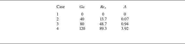
In table 4 we list the value of
 $\varLambda$
computed by (3.15) with the mean particle settling velocity obtained from the simulations. Not surprisingly,
 $\varLambda$
increases with the Galileo number because of the increased particle settling velocity. Also, it is noteworthy that the ratio is as low as
 $\varLambda =0.07$
for the case with
 ${\textit{Ga}}=40$
, indicating the negligible energy input by gravity sedimentation compared with the external forces. This is in agreement with the marginal difference regarding the SBS budgets between the cases with
 ${\textit{Ga}}=0$
and
 ${\textit{Ga}}=40$
(the red and cyan lines in figure 8). Nevertheless, increasing the Galileo number to
 ${\textit{Ga}}=80$
, the energy injection due to the particle sedimentation becomes comparable to that of the external forces with
 $\varLambda =0.94$
; the former contribution becomes the predominant mechanism of energy production at
 ${\textit{Ga}}=120$
when the contribution from the particle sedimentation exceeds the EP forces by a factor approximately 4 (
 $\varLambda =3.92$
).
Ratio
 $\varLambda$
between the energy input by the particle settling and by the external forces maintaining turbulence for the different cases under examination. See text for the definition of
 $ \varLambda$
in (3.15).

Comparison of the cumulative contributions to the SBS energy budget for the different Galileo number under consideration: (a) IBM forcing term; (b) nonlinear transfer; (c) viscous dissipation. Here we only present the data for
 $\kappa \gt \kappa _{\!f}$
.

We also observe from figure 8(a) that the large-scale energy transfer by the particle–fluid interactions, indicated by the negative slope of
 $\mathcal{F}_{\textit{ib}}^\varSigma (\kappa )$
in the suspensions with
 ${\textit{Ga}}=0$
and 40, becomes negligible at higher Galileo numbers. As discussed below, the decrease with
 ${\textit{Ga}}$
of the net energy removal by the settling particles at large scales is associated with a cancellation between the additional injection of energy into vertically elongated scales and the quenching of the horizontal flow correlations, so at the origin of the flow anisotropy. Furthermore, the range of scales on which the energy is injected by the particle–fluid interactions (region with positive slope of
 $\mathcal{F}_{\textit{ib}}^\varSigma (\kappa )$
) is enlarged when increasing the Galileo number.
The different behaviour of the particle–fluid interactions also alters the energy transport by the nonlinear terms. As shown in figure 8(b), this energy transfer is weakened as the Galileo number increases. For the greatest particle settling velocity at
 ${\textit{Ga}}=120$
, the contribution from the nonlinear transfer to the energy budget becomes subdominant compared with those from the particle–fluid interaction and the viscous dissipation (see figure 7
b). In other words, the energy input by the particle sedimentation is almost in direct balance with the viscous dissipation within a wide wavenumber range, i.e.
 $\mathcal{F}_{\textit{ib}} (\kappa ) \approx -\mathcal{D}_{\textit{ib}} (\kappa )$
, at
 ${\textit{Ga}}=120$
. This observation supports the local-balance assumption proposed by Lance & Bataille (Reference Lance and Bataille1991) regarding the pseudoturbulence induced by rising bubbles. In our recent study on the particle sedimentation in an initially quiescent fluid (Jiang et al. Reference Jiang, Brandt, Xu and Zhao2025), we also observed this local balance in the particle-induced pseudoturbulence, which leads to the
 $\kappa ^{-3}$
scaling of the energy spectra. Note, however, that this local balance is only observed at the smallest scales at lower
 ${\textit{Ga}}$
.
As regards the spherical-shell spectra of the viscous dissipation, we observe from figure 8(c) that
 $\mathcal{D}^\varSigma (\kappa ) \sim -\log (\kappa )$
on the scales close to the particle size, corresponding to the
 $E(\kappa ) \sim \mathcal{D}(\kappa )/\kappa ^2 \sim \kappa ^{-3}$
scaling of the energy spectra for the particle-laden flows shown in figure 6. Note, interestingly, that this scaling is not clearly observed in the particle-laden turbulence with
 ${\textit{Ga}}\leqslant 40$
(in absence of or with weak gravity sedimentation), when the local-balance mechanism only holds at the smallest scales.
To gain more insights on the small-scale dynamics, we further examine the energy budget at scales smaller than the particle size. Specifically, we compute the integrals of the nonlinear transfer term, IB forcing term and the viscous dissipation term at
 $\kappa \geqslant \kappa _d$
, denoted by
 \begin{align} {\varPi }^\lt =\sum \limits _{\kappa \geqslant \kappa _d} {\varPi }\left ( \kappa \right ), \quad \mathcal{F}^\lt _{\textit{ib}}=\sum \limits _{\kappa \geqslant \kappa _d} \mathcal{F}_{\textit{ib}}\left ( \kappa \right ), \quad \mathcal{D}^\lt =\sum \limits _{\kappa \geqslant \kappa _d} \mathcal{D}\left ( \kappa \right ). \end{align}
The physical interpretations of these three quantities are: (i)
 ${\varPi }^\lt$
the total nonlinear energy transfer by inertia from larger scales to subparticle scales; (ii)
 $\mathcal{F}^\lt _{\textit{ib}}$
the total energy contribution from the particle–fluid interactions at subparticle scales; (iii)
 $\mathcal{D}^\lt$
the total energy dissipation at subparticle scales. The values of
 ${\varPi }^\lt _{\textit{ib}}$
,
 $\mathcal{F}^\lt _{\textit{ib}}$
and
 $\mathcal{D}^\lt$
are shown in figure 9 for all cases being examined, normalized by the single-phase dissipation rate
 $\epsilon _0$
. Note first that the balance of the energy budget suggests
 $\mathcal{D}^\lt = -({\varPi }^\lt + \mathcal{F}^\lt _{\textit{ib}})$
, which is confirmed by the data shown in figure 9. In contrast to the single-phase turbulence with only the nonlinear transfer as energy source, the particle–fluid interaction always provides a net energy input at subparticle scales in the particle-laden cases. In other words, the IB forces do positive work at small scales, regardless of the Galileo number. As the Galileo number increases, the energy input by particle sedimentation is enhanced due to the greater particle settling velocity; the energy brought to small scales by nonlinear effects decreases in particle-laden flows with
 ${\textit{Ga}}\leqslant 40$
and then increases, remaining, however, lower than the input by the sedimentation at high
 ${\textit{Ga}}\geqslant 80$
. It is also interesting to note that the absolute value of
 ${\varPi }^\lt$
is larger than that of the single-phase turbulence at
 ${\textit{Ga}}=120$
. This indicates that the energy injection by the particle–fluid interaction, which starts at scales larger than the particle size (see the positive slope of
 $\mathcal{F}^\varSigma _{\textit{ib}}$
at
 $\kappa \lesssim \kappa _d$
in figure 8
a), would be partially transferred to small scales by inertial effects. The results shown in figures 8 and 9 suggest that more energy is available at
 $\kappa = \kappa _d$
at high
 ${\textit{Ga}}$
, which is sufficient to trigger nonlinear velocity fluctuations and to force an extension of the dissipative range towards smaller scales.
The energy budget at small scales (smaller than the particle size,
 $\kappa \geqslant \kappa _d$
) for the different suspension flows under investigation. The numbers on the horizontal axis represent the Galileo number, except for ‘SP’ standing for the single-phase turbulence.

The analysis of the SBS budget indicates how the combined effects of the particle-enhanced energy cascade (evident at
 ${\textit{Ga}}=0$
or 40) and the energy input by particle sedimentation (more evident at
 ${\textit{Ga}}=80$
or 120) alter the energy transfer path in the particle-laden turbulent flows. In particular, the energy transfer induced by the particle–fluid interactions quenches the classic inertia-driven energy cascade (characterized by
 $E(\kappa ) \sim \kappa ^{-5/3}$
in the inertial range), leading to a robust
 $\kappa ^{-3}$
scaling of the energy spectra. When settling is null or relatively weak, the local balance between fluid–structure interactions and dissipation is seen only at small scales. As soon as the settling speed (or equivalently the Galileo number) increases, the
 $\kappa ^{-3}$
scaling of the energy spectra appears on wider scale ranges, even at the largest flow scales, completely masking the classic
 $\kappa ^{-5/3}$
spectra for the highest
 ${\textit{Ga}}$
under the current investigation. Indeed, we notice the coexistence of the
 $\kappa ^{-5/3}$
and
 $\kappa ^{-3}$
scalings of the energy spectra at different scales in the suspensions with
 ${\textit{Ga}}=0$
and
 ${\textit{Ga}}=40$
(see the cyan and red lines in figure 6); in these flows, the modulation of the energy transfer by the particle–fluid interactions does not reach the inertial scales and remains limited to structures smaller than the particle size. A similar observation regarding the coexistence of inertia-dominated and fluid–structure-dominated dynamics underlying the energy spectrum was also reported in bubble-laden and particle-laden turbulent flows (Pandey, Mitra & Perlekar Reference Pandey, Mitra and Perlekar2023; Chiarini & Rosti Reference Chiarini and Rosti2024).
3.3.2. The spectral analysis on the two-dimensional plane
Energy spectral density in the
 $\kappa _h-\kappa _y$
plane. The notation
 $\tilde {E}^*$
denotes the normalized energy spectral density, i.e.
 $\tilde {E}^*=\tilde {E}/(E_k D^3)$
. The dashed grey contour lines depict the result for the particle-laden turbulence without particle sedimentation (
 ${\textit{Ga}}=0$
), while the coloured solid lines illustrate the result for (a,e) the single-phase flow, and the particle-laden flows with (b, f)
 ${\textit{Ga}}=40$
, (c,g)
 ${\textit{Ga}}=80$
and (d,h)
 ${\textit{Ga}}=120$
. The linear scale is used for the axes in (a–d) while the log scale is used in (e–h).

To further understand the directional information of the turbulence modulated by the settling particles, we analyse the energy budget on the two-dimensional
 $\kappa _h-\kappa _y$
plane, corresponding to horizontal and vertical wavenumbers. First, we present in figure 10 the two-dimensional distribution of the energy spectral density. Here, we display the data with linear scale in figure 10(a–d) to better illustrate the isotropy/anisotropy and with log scale on the bottom row to clarify the large-scale information. In each panel, we display with dashed lines the results pertaining to the suspension with
 ${\textit{Ga}}=0$
.
Figure 10(a,e) compare the single-phase turbulence with the particle-laden flow of neutrally buoyant particles. As expected, the energy distribution retains isotropy in the absence of particle sedimentation, as shown by the concentric-circle contour lines of
 $\tilde {E}^*$
with the linear scale of
 $\kappa _h$
and
 $\kappa _y$
(figure 10
a), or the diagonal-symmetric contour lines with the log-scale axes (figure 10
e). The presence of particles induces a slower decay of
 $\tilde {E}^*$
along the radial direction, i.e. an increase of energy at the smallest scales, which is in agreement with the raised spherical-shell energy spectrum below the particle scale shown in figure 6.
For the cases with non-zero Galileo numbers, we observe from figure 10(b–d, f–h) that the particle sedimentation breaks the isotropy of the energy distribution in the spectral space. The contour lines of
 $\tilde {E}^*$
are elongated along the
 $\kappa _h$
-direction on the scales close to or moderately smaller than the particle size (
 $\kappa _h \gtrsim \kappa _d$
), an observation becoming more prominent as the Galileo number increases. Specifically, for a given solid contour line at intermediate scales in figures 10(c) or 10(d), which represents flow structures with equal energy, we see that its intercept on the horizontal axis occurs at larger wavenumber than that on the vertical axis. This indicates the larger physical dimension of this flow structure along the vertical direction than the horizontal, and can be related to the local flow structures around the settling particles: thin shear layers and elongated wakes appear in the lateral and vertical directions, respectively (see also Fornari et al. Reference Fornari, Picano and Brandt2016a
). Note, however, that the contour lines of
 $\tilde {E}^*$
tend to recover symmetry far from the origin of the
 $\kappa _h-\kappa _y$
plane, indicating the recovery of the flow isotropy at small scales. As concerns the suspension at
 ${\textit{Ga}}=40$
, however, the anisotropy is hardly visible (figure 10
b, f). This can be ascribed to the marginal effect of particle sedimentation as the particle mean settling velocity is significantly smaller than the turbulent velocity fluctuations (
 $\langle V_s \rangle / u'=0.21$
) in this case.
Spectra of the IB forcing work in the
 $\kappa _h-\kappa _y$
plane for the particle-laden flows under investigation. The data is normalized by
 $\tilde {\mathcal{F}}_{\textit{ib}}^*=\tilde {\mathcal{F}}_{\textit{ib}}/(\mathcal{D}_{\textit{tot}}^\varSigma D^3)$
, and only positive values of
 $\tilde {\mathcal{F}}_{\textit{ib}}^*$
are illustrated by contour lines (denoted by the subscript ‘+’) . The dashed grey lines correspond to non-settling particles (
 ${\textit{Ga}}=0$
), while the coloured solid lines illustrate the results for (a)
 ${\textit{Ga}}=40$
, (b)
 ${\textit{Ga}}=80$
and (c)
 ${\textit{Ga}}=120$
. Log-scale axes are used. The symbols
 and
 indicates the region with negative values of
 $\tilde {\mathcal{F}}_{\textit{ib}}^*$
and the position of the positive peak of
 $\tilde {\mathcal{F}}_{\textit{ib}}^*$
.

Same as figure 11 but for the two-dimensional spectra of the nonlinear term
 $\tilde {{\varPi }}$
.

Next, we present the two-dimensional contours of the spectral density associated with the IB forcing in figure 11 and with the nonlinear term in figure 12. In each panel, the results pertaining to a non-zero settling velocity are compared with the case of
 ${\textit{Ga}}=0$
. As shown in figure 11(a) with the results at
 ${\textit{Ga}}=0$
and 40, the particle–fluid interactions mainly transfer energy from large to small scales along the radial direction in the spectral space so the flow anisotropy is hardly visible; in particular, the directional bias of
 $\tilde {\mathcal{F}}_{\textit{ib}}$
is null for the case with
 ${\textit{Ga}}=0$
and very weak for
 ${\textit{Ga}}=40$
. However, when the effect of particle sedimentation becomes significant with the increase of
 ${\textit{Ga}}$
to 80 and 120, we observe a clear positive peak of
 $\tilde {\mathcal{F}}_{\textit{ib}}$
around
 $\kappa _h \approx 0.3-0.6\kappa _d$
for low values of
 $\kappa _y$
, indicated by the symbol
 in figure 11(b,c), a signature of the energy injection by the settling particles. We therefore demonstrate that the energy input by the gravitational sedimentation is anisotropic in the spectral space, unlike the isotropic large-scale energy injection by the external EP forces. This mechanism is responsible for the anisotropic energy distribution shown in figure 10(c,d,g,h). Note also that, the region of the spectral space characterized by negative values of
 $\tilde {\mathcal{F}}_{\textit{ib}}$
(marked by
 in figure 11), indicating energy removal by the particle–fluid interactions, loses its isotropy at large scales as
 ${\textit{Ga}}$
increases. This is associated with the aforementioned positive peak of
 $\tilde {\mathcal{F}}_{\textit{ib}}$
as well. The increased energy injection by particle sedimentation partially cancels out the particle-induced energy transfer from large to small scales, which leads to a decreased energy removal by the IB forces at low wavenumbers (see figure 8
a). Additionally, the anisotropic energy input by the particle sedimentation becomes more pronounced for higher
 ${\textit{Ga}}$
, along with the positive value of
 $\tilde {\mathcal{F}}_{\textit{ib}}$
expanding to lower wavenumbers. To sum up, the settling particles induce flow anisotropy by forcing vertically elongated structures while breaking the flow coherence in the horizontal direction; this only leads to the weakened energy injection/removal at large scales when examining the spherical-shell energy spectra, yet leaves an imprinting on the flow (its anisotropy).
To conclude this section, let us elaborate on the two-dimensional spectrum of the energy transfer by nonlinear terms, with the results shown in figure 12. Similar to figure 10(a,e) and figure 11(a), the two-dimensional plot of
 $\tilde {{\varPi }}$
retains isotropy on the
 $\kappa _h-\kappa _y$
plane for the particle-laden flows with
 ${\textit{Ga}}=0$
and
 ${\textit{Ga}}=40$
(figure 12
a). Increasing the particle settling speed,
 $\tilde {{\varPi }}$
exhibits anisotropy in the cases at
 ${\textit{Ga}}=80$
and 120 (figures 12
b and 12
c), which can be seen as a consequence of the anisotropic energy input by the particle–fluid interactions (the IB forcing term).
It is interesting to note the negative peak of
 $\tilde {{\varPi }}$
on the horizontal axis at
 $\kappa _h \approx 0.5\kappa _d$
for the
 ${\textit{Ga}}=120$
case, highlighted by the symbol
 in figure 12(c). This indicates the removal of energy by the nonlinear effect at these intermediate scale, as also indicated by the negative slope of
 ${\varPi }^\varSigma (\kappa )$
for the associated case at
 $\kappa \approx 0.3\kappa _d-0.5\kappa _d$
in figure 8(b). Notice also that the location of the negative peak of
 $\tilde {{\varPi }}$
in figure 12(c) coincides with the positive peak of
 $\tilde {\mathcal{F}}_{\textit{ib}}$
shown in figure 11(c). Therefore, for the flow with a substantial energy supply from the particle sedimentation, part of the energy input by the particle–fluid interaction is transferred outwards at intermediate scales by the nonlinear effects. This is analogy to the energy extraction by inertial effects at large scales for the single-phase turbulence.
3.4. Particle clustering and collision rate
3.4.1. Voronoi analysis
In this section, we examine the spatial clustering and collision rate of the dispersed particles in the turbulent flows. To begin with, we employ the Voronoi analysis to investigate the particle spatial distribution (Monchaux, Bourgoin & Cartellier Reference Monchaux, Bourgoin and Cartellier2010). With this analysis tool, the domain is partitioned into Voronoi tessellations of the same number of particles, such that any point in one tessellation is closest to the associated particle. In figure 13(a) we present the probability distribution of the volumes of the Voronoi tessellations in each particle-laden case under study. The symbol
 $\overline {V}_{Voro}$
denotes the Voronoi volume
 ${V}_{Voro}$
normalized by the mean value for the same particle concentration,
 $\langle {V}_{Voro} \rangle = V_{\varOmega }/N_{\!p}$
. Note that we also show the data for the randomly distributed non-overlapping particles at the same volume fraction
 $\phi =10\,\%$
for the sake of comparison. The statistics for the randomly distributed particles are collected by repeatedly generating non-overlapping particles with a Poisson process (Uhlmann Reference Uhlmann2020). The data in the figure reveal that the PDF of
 $\overline {V}_{Voro}$
is more intermittent in HIT than for the random spatial distribution, indicating the occurrence of particle clustering (Monchaux et al. Reference Monchaux, Bourgoin and Cartellier2010).
To quantify the degree of particle clustering, we compute the standard deviation of the normalized Voronoi volumes,
 $\sigma (\overline {V}_{Voro})$
, and define the clustering indicator
 $C$
as the ratio
 $\sigma (\overline {V}_{Voro})$
to that of the randomly distributed particles (Tagawa et al. Reference Tagawa, Roghair, Prakash, Van Sint Annaland, Kuipers, Sun and Lohse2013):
 \begin{equation} C=\sigma (\overline {V}_{Voro})/\sigma (\overline {V}_{Voro}^{rand}). \end{equation}
As shown in figure 13(b), the value of
 $C$
is greater than unity in each case but does not change much with the Galileo number, which is consistent with the PDFs shown in figure 13(a). In previous studies, heavy, finite-size particles (without sedimentation) were reported to exhibit clustering in HIT (Fiabane et al. Reference Fiabane, Zimmermann, Volk, Pinton and Bourgoin2012; Uhlmann & Chouippe Reference Uhlmann and Chouippe2017; Chiarini & Rosti Reference Chiarini and Rosti2024), unlike neutrally buoyant particles (Fiabane et al. Reference Fiabane, Zimmermann, Volk, Pinton and Bourgoin2012). Nevertheless, particles settling in an otherwise quiescent fluid (without background turbulence) were not observed to cluster in both dilute and non-dilute suspensions at
 ${\textit{Ga}}=80$
(Jiang et al. Reference Jiang, Brandt, Xu and Zhao2025, Reference Jiang, Zhao and Brandt2026). Therefore, turbulence transport, instead of particle sedimentation, plays an essential role in the clustering of finite-size particles; the so-called ‘sweep-stick’ mechanism (Goto & Vassilicos Reference Goto and Vassilicos2008), i.e. particles preferentially accumulate in weak-fluid-acceleration regions (sticky points), is considered responsible for the particle clustering in most scenarios (Uhlmann & Chouippe Reference Uhlmann and Chouippe2017; Chiarini & Rosti Reference Chiarini and Rosti2024). This may explain the weak variation of the particle clustering intensity with the particle settling velocity, as shown by the data presented in figure 13(b). Moreover, in figure 13(b) we also quantitatively compare the clustering indicator from the present data with earlier studies. The discrepancy suggests the sophisticated dependence of the particle clustering on the particle properties, in agreement with the conclusion in Chiarini & Rosti (Reference Chiarini and Rosti2024). In particular, the effect of particle sedimentation on the clustering of finite-size particles in HIT remains to be further explored. Note, additionally, that the clustering was found to contribute to the enhancement of particle settling (or bubble rising) velocity in dilute scenarios (Jiang et al. Reference Jiang, Xu and Zhao2024b
; Hessenkemper et al. Reference Hessenkemper, Bragg, Lucas and Ma2025). This effect appears to be negligible in the present set-up given the relatively high-volume fraction; the particle mean settling velocity is always lower than that of an isolated particle as discussed in § 3.2.
(a) Probability density function (PDF) of the normalized Voronoi volumes of the dispersed particles. (b) The clustering indicator
 $C$
versus the Galileo number
 ${\textit{Ga}}$
. The present results (indicated by
 $\bullet$
) are compared with previous studies, (
 $\blacksquare$
) heavy particles in HIT (
 $\rho _{\!p}/\rho _{\!f}=1.5$
,
 $D/\eta = 11$
,
 $\phi =0.5\,\%$
) (Uhlmann & Chouippe Reference Uhlmann and Chouippe2017); (
 $\blacktriangle$
) heavy particles in HIT (
 $\rho _{\!p}/\rho _{\!f}=1.29$
,
 $D/\eta = 16$
,
 $\phi =7.9\,\%$
) (Chiarini & Rosti Reference Chiarini and Rosti2024); (
 $\blacklozenge$
) settling particles in the otherwise quiescent fluid (
 $\rho _{\!p}/\rho _{\!f}=2$
,
 $\phi =5\,\%$
) (Jiang et al. Reference Jiang, Zhao and Brandt2026).

3.4.2. Collision kernel and the particle pair statistics
Another issue we are concerned with is the collision rate of the dispersed particles, which is relevant to a variety of physical processes in environmental and industrial applications (Pumir & Wilkinson Reference Pumir and Wilkinson2016). In a variety of existing studies, the collision kernel
 $\varGamma$
is employed to quantify the collision rate in a particulate system (Smoluchowski Reference Smoluchowski1917; Saffman & Turner Reference Saffman and Turner1956; Pumir & Wilkinson Reference Pumir and Wilkinson2016; Wang Reference Wang, Subramaniam and Balachandar2023). For the monodisperse system, the collision kernel is defined as the rate of collision events normalized by the square of the particle number density (Wang, Wexler & Zhou Reference Wang, Wexler and Zhou2000),
 \begin{equation} \varGamma = 2\dot {N}_C/n^2. \end{equation}
Here,
 $\dot {N}_C$
denotes the number of collision events per unit volume and per unit time, and
 $n=N_{\!p}/V_{\varOmega }$
is the particle number density. To obtain
 $\varGamma$
, we count the number of collision events within the statistically steady state during the simulations and then compute the collision kernel by its definition (3.18). As shown in figure 14, the collision kernel
 $\varGamma$
, normalized by the single-phase r.m.s. velocity
 $u'_0$
, first decreases slightly with the introduction of particle sedimentation at
 ${\textit{Ga}}=40$
, and then increases when further increasing
 ${\textit{Ga}}$
.
To better examine the combined effect of sedimentation and turbulent transport on the collision rate, we compare the present results with the particle collision kernel in the absence of background turbulence. In our previous study on the particle sedimentation in an initially quiescent fluid (Jiang et al. Reference Jiang, Zhao and Brandt2026), the collision kernel, normalized by the single-particle settling velocity, was found to be
 $\varGamma /(V_{s0}D^2)=0.29$
at
 ${\textit{Ga}}=80$
– a value obtained at a volume fraction
 $\phi =5\,\%$
but found to be insensitive to the particle volume fraction. If we similarly normalize the collision kernels by
 $V_{s0}$
for the present cases, we can obtain the results of
 $\varGamma /(V_{s0}D^2)$
as listed in table 5. For the same
 ${\textit{Ga}}=80$
the collision kernel is increased by approximately 4.75 times in the present turbulent flow when compared with that in the quiescent fluid (Jiang et al. Reference Jiang, Zhao and Brandt2026). Additionally, the value of
 $\varGamma /(V_{s0}D^2)$
decreases considerably as
 ${\textit{Ga}}$
increases due to the increase of
 $V_{s0}$
, which is in contrast to the weak variation of
 $\varGamma /(u'_0 D^2)$
with
 ${\textit{Ga}}$
. Thus, we can conclude that the turbulent transport is the dominant effect for particle collisions in the present flow configuration.
Collision kernel normalized by the single-particle settling velocity.

Collision kernel normalized by the r.m.s. velocity fluctuation of the single-phase turbulence as a function of
 ${\textit{Ga}}$
.

Finally, we attempt to interpret the variations in the collision kernel with the Galileo number shown in figure 14. To this end, we introduce the kinematic description of the collision kernel (Wang et al. Reference Wang, Wexler and Zhou2000; Wang Reference Wang, Subramaniam and Balachandar2023),
 \begin{equation} \varGamma ^K=2\pi R^2 \langle |W_r(R)| \rangle g (R). \end{equation}
Here,
 $R=D$
is the collision radius, and
 $\langle |W_r(R)| \rangle$
and
 $g(R)$
represent the mean absolute RRV and the RDF for particles at the separation distance
 $r=R$
. Readers can refer to Wang et al. (Reference Wang, Wexler and Zhou2000) for the definitions of RRV and RDF presented in (3.19). To provide a physical interpretation, the kinematic collision
 $\varGamma ^K$
is the flux of particles across a collision sphere centred at the reference particle with a collision radius
 $R=D$
. The RRV provides the information of the relative motion among particles, whereas the RDF reflects the particle spatial distribution by measuring the probability of finding particles pairs with a given separation distance. Theoretically, the kinematic collision kernel
 $\varGamma ^K$
is equivalent to the dynamic collision kernel
 $\varGamma$
defined in (3.18) (Wang et al. Reference Wang, Wexler and Zhou2000).
(a) Radial distribution function (RDF) and (b) relative radial velocity (RRV) of the dispersed particles as function of the separation distance
 $r$
. The inset panels are the zoom-in view close to
 $r=D$
. The RDF of randomly distributed non-overlapping particles (the hard-sphere distribution, see Liu (Reference Liu2024)) is displayed in panel (a) with dashed line for comparison.

(a,b) The particle pair distribution function and (c,d) relative particle velocity at (a,c)
 ${\textit{Ga}}=0$
and (b,d)
 ${\textit{Ga}}=120$
as function of the distance
 $r$
and the angle
 $\psi$
.

In figure 15, we display the RDF and RRV as functions of the particle separation distance
 $r$
. As shown in figure 15(a), the RDF exhibits a pronounced peak at
 $r=D$
; this peak indicates the enhanced probability of finding touching particle pairs in the turbulent flow compared with randomly distributed particles. As the separation distance
 $r$
increases, the RDF quickly decreases to
 $g(r)=1$
, indicating a rapid decorrelation of particle locations. As regards the RRV,
 $\langle |W_r| \rangle$
is directly related to the particle velocity fluctuations for the largest separation distances (Jiang et al. Reference Jiang, Zhao and Brandt2026), so the value of
 $\langle |W_r| \rangle$
at
 $r \gtrsim 3D$
decreases with the Galileo number (shown in figure 15
b) owing to the reduced particle velocity fluctuations (see figure 5
a). At small separations, instead, the particle relative motion is dominated by the interparticle hydrodynamic interactions. The RRV decreases rapidly as the separation distance approaches
 $r \approx D$
owing to the significant lubrication effects among nearby particles (Jiang et al. Reference Jiang, Xu and Zhao2024b
). In addition, it is noteworthy that the value of
 $\langle |W_r (r=D)| \rangle$
is highest at
 ${\textit{Ga}}=120$
among all cases, which explains the highest collision kernel shown in figure 14 for the highest-
 ${\textit{Ga}}$
case, although the value of
 $g(r=D)$
is slightly reduced at
 ${\textit{Ga}}=120$
(see the inset in figure 15
a).
At last, to further examine the effect of gravity on the particle-pair dynamics, we compute the particle-pair correlation function
 $g(r,\psi )$
and the absolute RRV
 $|W_r(r,\psi )|$
as two-dimensional functions of the independent variables
 $r$
(the radial separation) and
 $\psi$
(the polar angle relative to the vertical direction). This allows us to further understand the directional information about the particle spatial distribution and relative motions. Note that one can obtain the one-dimensional functions
 $g(r)$
and
 $\langle |W_r(r)|\rangle$
by integrating
 $g(r,\psi )$
and
 $|W_r(r,\psi )|$
over the polar angle
 $\psi$
as (Yin & Koch Reference Yin and Koch2007)
 \begin{align} g(r) &= \frac {1}{2}\int _0^\pi {g(r,\psi )\sin \psi {\rm d}\psi }, \end{align}
 \begin{align} \langle |W_r(r)|\rangle &= \frac {1}{2}\int _0^\pi {|W_r(r,\psi )| g(r,\psi ) \sin \psi {\rm d}\psi }. \end{align}
The functions
 $g(r,\psi )$
and
 $|W_r(r,\psi )|$
are depicted in figure 16 for the suspensions at
 ${\textit{Ga}}=0$
(no gravity) and
 ${\textit{Ga}}=120$
(strongest particle sedimentation). As shown in figure 16(a,c),
 $g(r,\psi )$
and
 $|W_r(r,\psi )|$
only vary with the radial separation
 $r$
for non-sedimenting particles (
 ${\textit{Ga}}=0$
), and do not exhibit any directional preference. In contrast, at
 ${\textit{Ga}}=120$
, we can clearly observe a directional bias in the spatial distribution and relative motion of particle pairs due to the sedimentation. Specifically, the data in figure 16(b) show that the probability of finding particle pairs along the horizontal direction is higher than that in the vertical direction, which could be related to the wake-induced hydrodynamic interactions among settling particles. This observation reminds us of the horizontally aligned particles settling in a quiescent fluid at a low Galileo number
 ${\textit{Ga}}\approx 18$
(Yin & Koch Reference Yin and Koch2007), but is in contrast to the column-like particle structures observed in settling-particle suspensions at high
 ${\textit{Ga}}$
(Uhlmann & Doychev Reference Uhlmann and Doychev2014). The different behaviours may be ascribed to the complexity of the DKT-like interactions at different particle Reynolds numbers or in the turbulent/non-turbulent environments.
Regarding the particle relative motion (cf. figure 16
d), the value of
 $|W_r(r,\psi )|$
is found to be greater for the horizontally aligned particle pairs (
 $\psi =90^\circ$
) than for the vertically aligned ones (
 $\psi =90^\circ$
) with a given radial separation distance
 $r$
. Note that the directional preference of
 $|W_r(r,\psi )|$
observed in the current study is opposite to that observed for settling particles in a quiescent fluid:
 $|W_r(r,\psi )|$
was found to be greater along the vertical direction than horizontal direction for settling particles in the absence of background turbulence (see e.g. figure 8e in Jiang et al. Reference Jiang, Zhao and Brandt2026). This difference is reminiscent of the opposite variation of the particle vertical velocity fluctuations as
 ${\textit{Ga}}$
increases in turbulent and quiescent fluids (see the discussion in § 3.2). The decrease of
 $\sigma (v_y)$
at
 ${\textit{Ga}}=120$
(see figure 5
a) is related to the smaller particle relative velocities along the vertical direction shown in figure 16(d), since the particle vertical velocity fluctuations can promote relative motion between the vertical-aligned particles. Moreover, considering the relationship (3.21), the large values of
 $g(r,\psi )$
and
 $|W_r(r,\psi )|$
in the region
 $(r,\psi ) \approx (D,90^{\circ })$
explain the higher value of
 $\langle |W_r(r=D)|\rangle$
in the suspension with
 ${\textit{Ga}}=120$
than for the non-sedimenting particles; this also results in an enhanced collision rate in the presence of gravitational sedimentation.
4. Concluding remarks
In this work, we have studied the gravity-driven sedimentation of spherical particles in sustained homogeneous and isotropic turbulence and the related turbulent modulation using PR-DNS. The particle size is an order of magnitude larger than the Kolmogorov length scale of the single-phase turbulent flow and the suspension volume fraction is fixed at 10 %. The effect of the particle sedimentation is studied by varying the value of the Galileo number of settling particles, which is achieved by changing the particle–fluid density ratios.
By computing the statistics of the turbulent flow, we find a reduced turbulence Taylor Reynolds number with the increase of the particle sedimentation speed because of the enhanced viscous dissipation induced by settling particles. The vorticity structures become fragmented, as confirmed by reduced Kolmogorov length scales, as the Galileo number increases. The interactions between settling particles and the turbulent flow result in higher fluid velocity fluctuations along the vertical direction than the horizontal one. Interestingly, the opposite is true for the velocity fluctuations of the solid phase: the reduced particle vertical velocity fluctuations are explained by the filtering of the background turbulent structures by the particle settling motions. Moreover, the average settling velocity of the particle phase is found to decrease when compared with that of the isolated settling particle in a quiescent fluid. The combined effects of hindrance in suspension and of the turbulence-induced drag increase are the reasons for the sedimentation attenuation. The latter effect becomes weaker as the ratio of the particle settling velocity to the turbulence velocity fluctuation velocity increases, i.e. increasing
 ${\textit{Ga}}$
.
To further explore the energy transfer of the turbulence modulated by particles, we have also investigated the energy spectra and SBS energy budget of the turbulent flows in the spectral space. Compared with the single-phase turbulence, the particles extract energy from large scales and reinject it at small scales, i.e. we observe a complementary energy cascade caused by the particle–fluid interactions, as in the bubble/droplet laden flows without gravity. This is shown by the presence of the
 $\kappa ^{-3}$
scaling of the energy spectra close to the particle scale. With the introduction of gravitational sedimentation, the settling motion of the particle phase plays an additional role in injecting energy into the fluid flow. The energy input by the particle sedimentation is proportional to the square of the Galileo number, and becomes the major energy source for the case with the highest Galileo number
 ${\textit{Ga}}=120$
, approximately four times the energy injected by the large-scale external forces. In addition, as the Galileo number increases, the
 $\kappa ^{-3}$
scaling of the energy spectra is seen over a wider range of scales, cancelling the classic energy cascade (characterized by the
 $\kappa ^{-5/3}$
scaling) in the inertial range at
 ${\textit{Ga}}=120$
. The
 $\kappa ^{-3}$
scaling of the energy spectra is found to be associated with an almost direct balance between the energy injection by the fluid–solid interactions and viscous dissipation.
To better understand the directional information of the turbulence modulation, the spectral analyses of the energy and its SBS budget analysis are also performed in cylinder coordinates in spectral space. With the introduction of the particle sedimentation, the interactions between settling particles and the carrier flows break the isotropy of the energy distribution, which is seen in the single-phase turbulence or the non-sedimenting particle-laden turbulence. This kind of anisotropy is characterized by the slow decay of the energy spectral density along the horizontal wavenumber on large scales, and is related to the flow structures induced by settling particles. In particular, the settling particles create elongated vertically aligned wakes while disrupting the horizontal correlations of the flow structures when falling through them. Nevertheless, the flow recovers isotropy at small scales. In the cases where the particle sedimentation is non-negligible, the energy input by the particle sedimentation is maximized near the particle scale. For a sufficiently high particle settling speed, the energy injected by this mechanism is also found to be transferred outwards by the nonlinear effect at intermediate scales.
At last, we have also investigated the spatial distribution and collision rate of the dispersed particles. By means of the Voronoi tessellation analysis, we identity a moderate particle clustering in the turbulent flow, a phenomenon hardly affected by the particle sedimentation. As regards the particle collision rate, the collision kernel is found to vary non-monotonically, yet not considerably in absolute value, with increasing Galileo number. Further examination of the particle pair statistics, i.e. the RDF and the RRV (only functions of the particle relative distance), reveals that the increased particle collision rate at high
 ${\textit{Ga}}$
is mainly caused by the enhanced particle–particle relative motions. By scrutinizing the particle pair statistics as function of distance and angle with respect to the gravity direction, we find that, when sedimentation is significant, nearby particle pairs tend to align horizontally under the interparticle hydrodynamic interactions. These horizontally arranged particle pairs tend to have greater relative motions than those aligned vertically, which explains the enhanced RRV of nearby particle pairs at a high Galileo number. This also demonstrates the importance of a complete anisotropic analysis to unveil the features of particle dynamics.
To conclude, in this paper, we have demonstrated the essential role of the gravitational sedimentation in the modulation of the particle-laden turbulent flows. However, we have only studied the effect of particle sedimentation by changing the particle density. The other relevant effects, like the particle size, particle inertia, volume fraction and particle shape (Voth & Soldati Reference Voth and Soldati2017; Peng et al. Reference Peng, Sun and Wang2023), are not addressed in the current work. In particular, whether the small-scale Kolmogorov scaling of the energy spectra (as shown in the bubble-induced turbulence by Ma et al. (Reference Ma, Tan, Ni, Hessenkemper and Bragg2025)) will appear in particle-laden turbulence at high Galileo numbers, as well as its potential interaction with the background turbulence, needs to be explored. Additionally, how the turbulence modulation is altered by the clustering of settling particles at high
 ${\textit{Ga}}$
but low
 $\phi$
(see e.g. Chouippe & Uhlmann Reference Chouippe and Uhlmann2019) remains unknown. Finally, it is of interest to examine the potential usefulness of the non-dimensional parameter
 $\varLambda$
(see (3.15)) to predict turbulence modulation in such scenarios. Moreover, the change of the local flow topology by the presence of settling particles (see recent studies by Chiarini & Rosti (Reference Chiarini and Rosti2024) and Chiarini et al. (Reference Chiarini, Tandurella and Rosti2025)) is worthy of further examination in future studies.
Funding
This research was funded by the Department of Energy and Process Engineering, Norwegian University of Science and Technology (NTNU), Norway and by Politecnico di Torino, Italy.
Declaration of interests
The authors report no conflict of interest.
Appendix A. Particle budget
In this appendix, we provide the detailed derivation of (3.13). As introduced in the main text, the contribution from the fluid–particle interactions to the total fluid-energy budget is caused by the work of the IBM forces, i.e.
 \begin{equation} \varPsi _{p}=\left \langle {{\boldsymbol{f}}_{\!\textit{ib}}} \boldsymbol{\cdot }{\boldsymbol{u}} \right \rangle _\varOmega . \end{equation}
To establish the link between
 $\varPsi _p$
and the particle dynamics, we reformulate the equation above as follows (Chouippe & Uhlmann Reference Chouippe and Uhlmann2015):
 \begin{equation} \begin{aligned} \varPsi _{p} & =\left \langle \boldsymbol{f}_{\!\textit{IB}}\boldsymbol{\cdot }\boldsymbol{u}\right \rangle _\varOmega \\ & =\frac {1}{V_\varOmega }\int _\varOmega \boldsymbol{f}_{\!\textit{IB}}\boldsymbol{\cdot }\boldsymbol{u}{\rm d}\varOmega \\ & \approx \frac {1}{V_\varOmega }\sum _{i=1}^{N_{\!p}}\int _{\partial \varOmega _p^i}\boldsymbol{F}_{\!\textit{IB}}^i\boldsymbol{\cdot }\boldsymbol{U}^i{\rm d}S. \end{aligned} \end{equation}
Here, the capitalized variables represent Lagrangian quantities defined on the Lagrangian points on the particle surface, and the superscript
 $i$
(
 $i=1,2,\boldsymbol{\cdot}s ,N_{\!p}$
) denotes the specific particle. The conservation of momentum between the Eulerian and the Lagrangian representations of the IBM forces is applied for the derivation above (Peskin Reference Peskin2002; Breugem Reference Breugem2012), and the surface velocity
 $\boldsymbol{U}^i$
is computed by the rigid-motion of the particle,
 \begin{equation} \boldsymbol{U}^i=\boldsymbol{v}_p^i+\boldsymbol{\omega }^i\times \boldsymbol{r}, \end{equation}
where
 $\boldsymbol{r}=\boldsymbol{X}-\boldsymbol{x}_c^i$
is the vector from the particle centroid to a point on the particle surface. By inserting (A3) into (A2) and using the relationship
 $\phi =N_{\!p} V_{\!p} /V_\varOmega$
and
 $(\boldsymbol{\omega }_p\times \boldsymbol{r})\boldsymbol{\cdot }\boldsymbol{F_{IB}}=\boldsymbol{\omega }_p\boldsymbol{\cdot }( \boldsymbol{r}\times \boldsymbol{F_{IB}})$
, we arrive at
 \begin{equation} \begin{aligned} \varPsi _{p} & \approx \frac {1}{V_{\varOmega }}\sum _{i=1}^{N_{p}}\int _{\partial \varOmega _{p}^{i}}\boldsymbol{F}_{\!\textit{IB}}^{i}\boldsymbol{\cdot }\boldsymbol{U}^{i}{\rm d}S \\ & =\frac {\phi }{V_{\!p}}\frac {1}{N_{p}}\sum _{i=1}^{N_{p}}\left [\boldsymbol{v}^{i}\boldsymbol{\cdot }\int _{\partial \varOmega _{p}^{i}}\boldsymbol{F}_{\!\textit{IB}}^{i}{\rm d}S+\boldsymbol{\omega }^{i}\boldsymbol{\cdot }\int _{\partial \varOmega _{p}^{i}}\boldsymbol{r}\times \boldsymbol{F}_{\!\textit{IB}}^{i}{\rm d}S\right ] \\ & = \frac {\phi }{V_{\!p}} \left \langle \boldsymbol{v}\boldsymbol{\cdot }\int _{\partial \varOmega _{p}}\boldsymbol{F}_{\!\textit{IB}}{\rm d}S + \boldsymbol{\omega }\boldsymbol{\cdot }\int _{\partial \varOmega _{p}}\boldsymbol{r}\times \boldsymbol{F}_{\!\textit{IB}}{\rm d}S \right \rangle _p . \end{aligned} \end{equation}
To proceed, let us reintroduce the Newton–Euler equations ((2.3)–(2.4)),
 \begin{align} \rho _{\!p} V_{\!p} \frac {\mathrm{d} \boldsymbol{v}}{\mathrm{d} t}&=- \!\int _{\partial \varOmega _p} \rho _{\!f} \boldsymbol{F}_{\!\textit{IB}} \mathrm{d}S + \rho _{\!f} \frac {{d}}{\mathrm{d}t} \int _{\varOmega _f} \boldsymbol{u} \mathrm{d}V - \!\int _{\varOmega _p}\! \rho _{\!f} \boldsymbol{f}_{\!\textit{ext}} {\rm d}V+\left (\rho _{\!p}-\rho _{\!f}\right ) \boldsymbol{g} V_{\!p}+\boldsymbol{F}_{\!C} \end{align}
 \begin{align} I_{\!p}\frac {\mathrm{d} \boldsymbol{\omega }}{\mathrm{d} t}&=-\rho _{\!f} \oint _{\partial \varOmega _p^i} \boldsymbol{r} \times \boldsymbol{F}_{\!\textit{IB}} {\rm d}S + \rho _{\!f} \frac {d}{{\rm d}t} \int _{\varOmega _p} \boldsymbol{r} \times \boldsymbol{u} {\rm d}V+\boldsymbol{T}_{\!C} . \end{align}
In the above equations, the hydrodynamic force (
 $\boldsymbol{F}_{\!H}$
) and torque (
 $\boldsymbol{T}_{\!H}$
) are replaced by the integral of the IBM forces obtained by integrating the momentum (2.2) over the volume occupied by the particle (Breugem Reference Breugem2012),
 \begin{align} \boldsymbol{F}^H &= \int _{\partial \varOmega _p} \boldsymbol{\tau } \boldsymbol{\cdot }\boldsymbol{n} \mathrm{d}S \nonumber\\ &= - \rho _{\!f} \int _{\partial \varOmega _p} \boldsymbol{F}_{\!\textit{IB}} \mathrm{d}S + \rho _{\!f} \frac {d}{{\rm d}t} \int _{\varOmega _{p(t)}} \boldsymbol{u} \mathrm{d}V - \rho _{\!f}\int _{\varOmega _p} \boldsymbol{f}_{\!\textit{ext}} \mathrm{d}V, \end{align}
 \begin{align} \boldsymbol{T}_{\!H} &= \int _{\partial \varOmega _p} \boldsymbol{r} \times \boldsymbol{\tau } \boldsymbol{\cdot }\boldsymbol{n} \mathrm{d}S \nonumber\\ &= -\rho _{\!f}\int _{\partial \varOmega _p} \boldsymbol{r} \times \boldsymbol{F}_{\!\textit{IB}} \mathrm{d}S + \rho _{\!f} \frac {{d}}{\mathrm{d}t} \int _{\varOmega _p} \boldsymbol{r} \times \boldsymbol{u} \mathrm{d}V - \rho _{\!f} \int _{\varOmega _p} \boldsymbol{r} \times \boldsymbol{f}_{\!\textit{ext}} \mathrm{d}V. \end{align}
Note that the external forces needed to sustain the turbulence (i.e. the last term in the above two equations) also contributes to the hydrodynamic force and torque on the particle, since the forcing term
 $\boldsymbol{f}_{\!\textit{ext}}$
is also applied in the space occupied by the dispersed particles.
By multiplying (A5) with the particle velocity
 $\boldsymbol{v}$
and computing the average over all particles, we can write
 \begin{equation} \begin{aligned} \rho _{\!p}V_{\!p}\frac {{d}}{\mathrm{d}t}\left \langle \frac {1}{2}\boldsymbol{v}\boldsymbol{\cdot }\boldsymbol{v}\right \rangle _{p}&=-\rho _{\!f}\left \langle \boldsymbol{v}\boldsymbol{\cdot }\int _{\partial \varOmega _{p}}\boldsymbol{F}_{\!\textit{IB}}\mathrm{d}S\right \rangle _{p}+\rho _{\!f}\left \langle \boldsymbol{v}\boldsymbol{\cdot }\frac {{d}}{\mathrm{d}t}\int _{\varOmega _{p}}\boldsymbol{u}\mathrm{d}V\right \rangle _{p}\\ &\quad -\rho _{\!f}\left \langle \boldsymbol{v}\boldsymbol{\cdot }\int _{\varOmega _{p}}\boldsymbol{f}_{\!\textit{ext}}\mathrm{d}V\right \rangle _{p}+\left (\rho _{\!p}-\rho _{\!f}\right )\left \langle \boldsymbol{v}\right \rangle _{p}\boldsymbol{\cdot }\boldsymbol{g}V_{\!p}+\left \langle \boldsymbol{v}\boldsymbol{\cdot }\boldsymbol{F}_{\!C}\right \rangle _{p}. \end{aligned} \end{equation}
The above equation describes the contributions to the temporal evolution of the mean translational kinetic energy of the particle phase. If we now introduce the assumption of rigid-body motion for the flow inside the particle, the second term on the right-hand side of (A9) can be reformulated as (Uhlmann Reference Uhlmann2005)
 \begin{equation} {\rho _{\!f}}{\left \langle {{\boldsymbol{v}} \boldsymbol{\cdot }\frac { {d}}{{\textrm {d}t}}\int _{{\varOmega _p}} {\boldsymbol{u}} \textrm {d}V} \right \rangle _p} \approx {\rho _{\!f}}{\left \langle {{\boldsymbol{v}} \boldsymbol{\cdot }\frac {{\textrm {d}{\boldsymbol{v}}}}{{\textrm {d}t}}{V_{\!p}}} \right \rangle _p} = {\rho _{\!f}}{V_{\!p}}\frac {{d}}{{\textrm {d}t}}{\left \langle {\frac {1}{2}{\boldsymbol{v}} \boldsymbol{\cdot }{\boldsymbol{v}}} \right \rangle _p}. \end{equation}
By inserting (A10) into (A9), we obtain after some algebraic manipulations,
 \begin{equation} \begin{aligned} {\left \langle {{\boldsymbol{v}} \boldsymbol{\cdot }\int _{\partial {\varOmega _p}} {{{\boldsymbol{F}}_{\!\textit{IB}}}} \textrm {d}S} \right \rangle _p} \approx &\left ( {\frac {{{\rho _{\!p}}}}{{{\rho _{\!f}}}} - 1} \right ){V_{\!p}}\left [ {{{\left \langle {\boldsymbol{v}} \right \rangle }_p} \boldsymbol{\cdot }{\boldsymbol{g}} - \frac { {d}}{{\textrm {d}t}}{{\left \langle {\frac {1}{2}{\boldsymbol{v}} \boldsymbol{\cdot }{\boldsymbol{v}}} \right \rangle }_p}} \right ] \\&- {\left \langle {{\boldsymbol{v}} \boldsymbol{\cdot }\int _{{\varOmega _p}} {{{\boldsymbol{f}}_{\!\textit{ext}}}} \textrm {d}V} \right \rangle _p} + \frac {1}{{{\rho _{\!f}}}}{\left \langle {{\boldsymbol{v}} \boldsymbol{\cdot }{{\boldsymbol{F}}_{\!C}}} \right \rangle _p}. \end{aligned} \end{equation}
Similar steps can be performed for the rotational dynamics of the particles, yielding
 \begin{equation} \begin{aligned} {\left \langle {{\boldsymbol{\omega }} \boldsymbol{\cdot }\int _{\partial {\varOmega _p}} {{\boldsymbol{r}} \times {{\boldsymbol{F}}_{\!\textit{IB}}}} {\rm d}S} \right \rangle _p} = &\frac {1}{{{\rho _{\!p}}}}\left ( {1 - \frac {{{\rho _{\!p}}}}{{{\rho _{\!f}}}}} \right ){I_{\!p}}\frac {{d}}{{\mathrm{d}t}}{\left \langle {\frac {1}{2}{{\boldsymbol{\omega }}_p} \boldsymbol{\cdot }{{\boldsymbol{\omega }}_p}} \right \rangle _p} \\ &- {\left \langle {{\boldsymbol{\omega }} \boldsymbol{\cdot }\int _{{\varOmega _p}} {{\boldsymbol{r}} \times {{\boldsymbol{f}}_{\!\textit{ext}}}} {\rm d}V} \right \rangle _p} + \frac {1}{{{\rho _{\!f}}}}{\left \langle {{\boldsymbol{\omega }} \boldsymbol{\cdot }{{\boldsymbol{T}}_C}} \right \rangle _p}. \end{aligned} \end{equation}
Inserting (A11) and (A12) into (A4), we can finally arrive at
 \begin{align} {\varPsi _p} & \approx - \frac {\phi }{{\rho _{\!p}}{V_{\!p}}} \left ( {\frac {{{\rho _{\!p}}}}{{{\rho _{\!f}}}} - 1} \right )\left [ {{ \rho _{\!p}V_{\!p} \frac { {d}}{{\textrm {d}t}}{{\left \langle {\frac {1}{2}{\boldsymbol{v}} \boldsymbol{\cdot }{\boldsymbol{v}}} \right \rangle }_p}} + {I_{\!p}}\frac {{d}}{{\mathrm{d}t}}{\left \langle {\frac {1}{2}{{\boldsymbol{\omega }}_p} \boldsymbol{\cdot }{{\boldsymbol{\omega }}_p}} \right \rangle _p}} \right ] \nonumber\\ &\quad + \phi \left ( {\frac {{{\rho _{\!p}}}}{{{\rho _{\!f}}}} - 1} \right ){{\left \langle {\boldsymbol{v}} \right \rangle }_p} \boldsymbol{\cdot }{\boldsymbol{g}} + \frac {\phi }{{{\rho _{\!f}}{V_{\!p}}}}\left [ {{{\left \langle {{\boldsymbol{v}} \boldsymbol{\cdot }{{\boldsymbol{F}}_{\!C}}} \right \rangle }_p} + {{\left \langle {{\boldsymbol{\omega }} \boldsymbol{\cdot }{{\boldsymbol{T}}_C}} \right \rangle }_p}} \right ] \nonumber\\ &\quad - \frac {\phi }{{{V_{\!p}}}}{{\left \langle {{\boldsymbol{v}} \boldsymbol{\cdot }\int _{{\varOmega _p}} {{{\boldsymbol{f}}_{\!\textit{ext}}}{\rm d}V} + {\boldsymbol{\omega }} \boldsymbol{\cdot }\int _{{\varOmega _p}} {{\boldsymbol{r}} \times {{\boldsymbol{f}}_{\!\textit{ext}}}{\rm d}V} } \right \rangle }_p}, \end{align}
which is identical to (3.13) in the main text.
Appendix B. Discussion on the particle-induced dissipation
In this appendix, we further look into the particle-induced dissipation and examine the contribution from
 $\varPsi _p^{\textit{ext}}$
to the particle budget (see (3.13)). To this end, we conducted an additional simulation for the case with
 ${\textit{Ga}}=0$
(no sedimentation). The difference of this additional simulation (which is referred to as case 1A for brevity hereinafter) from case 1 reported in the main text is that we set the external forces used to sustain the background turbulence to zero in the volume occupied by the dispersed particles. In other words, the forcing term
 $\boldsymbol{f}_{\!\textit{ext}}$
in (2.2) is applied only in the region occupied by the fluid phase. To keep the energy input unchanged, we compensate the energy loss due to the spatial filtering of the external forces by amplifying the magnitude of the forcing by the factor
 $1/(1-\phi )$
(Peng et al. Reference Peng, Sun and Wang2023), i.e.
 $\epsilon ^*_{\textit{exc}}=( {1}/{1-\phi })\epsilon ^*_{\textit{inc}}$
, where
 $\epsilon ^*$
denotes the magnitude of the EP forces (see table 1) and the subscripts ‘
 $exc$
’ and ‘
 ${\textit{inc}}$
’ denote the exclusion or inclusion of the volume occupied by the solid phase. Note that, to run this additional case, we restart the simulation from the checkout data of the original case 1 at
 $t=32.94 T_e$
.
Figure 17 illustrates the time history of the Taylor Reynolds number in the simulation of cases 1 and 1A. We can observe an almost unchanged mean value of
 ${\textit{Re}}_\lambda$
before and after the restart of the simulation, suggesting a negligible effect of the specific way the external force is applied on the single-point statistics of the modulated turbulence.
Time history of the Taylor Reynolds number
 ${\textit{Re}}_\lambda$
for the case with
 ${\textit{Ga}}=0$
. The original simulation (with external forces applied inside the solid phase) ends at
 $t=32.94 T_e$
(displayed by the vertical dashed line). After this instant, the simulation is restarted with external forces of increased magnitude only in the volume occupied by the fluid phase. Time is normalized by
 $T_e=u'^2/\epsilon$
, the integral time scale pertaining to this case.

Most importantly, we compare the SBS budget of the turbulent flow under these two conditions, with the results shown in figure 18. The most relevant difference is the reduction of the contribution from the particle–fluid interactions, i.e. the term
 $\mathcal{F}_{\textit{ib}}^\varSigma$
, when the external forces are limited to the fluid phase (the red dashed line in figure 18). In particular, the value of
 $\mathcal{F}_{\textit{ib}}^\varSigma (\kappa =\kappa _{max})$
is almost zero in case 1A, indicating the zero net contribution from the particle–fluid interactions to the fluid energy budget. This observation is consistent with the result reported in Chiarini & Rosti (Reference Chiarini and Rosti2024) among others.
To elucidate the difference between case 1 and 1A, we revisit the particle budget given by (3.13). Since the external force is excluded from the space occupied by the dispersed particles in case 1A, the integrals defining the term
 $\varPsi _p^{\textit{ext}}$
become zero, leading to the vanishing value of
 $\varPsi _p^{\textit{ext}}$
. This is in contrast to the negative value of
 $\varPsi _p^{\textit{ext}}$
due to the positive correlation between the particle motion and large-scale external forces in case 1 as discussed in the main text. Note additionally that the small residual value of
 $\mathcal{F}_{\textit{ib}}(\kappa =\kappa _{max})$
in case 1A (see the last point of the red dashed line in figure 18
a) is related to the contribution from the particle–particle collisions (the term
 $\varPsi _p^{col}$
in (3.13)).
(a) Cumulative and (b) non-cumulative SBS energy budget for the suspension of spherical particles with
 ${\textit{Ga}}=0$
. The solid lines represent the results with the external forces needed to sustain the turbulence also applied inside the solid phase (the same as in figure 7
a), while the dashed lines are the results limiting these forces to the fluid phase. The total viscous dissipation
 $\mathcal{D}^\varSigma _{\textit{tot}}=-\sum_{\kappa = 0}^{{\kappa _{\textit{max}}}} {\mathcal{D}( \kappa )}$
is used to normalize the data.

By scrutinizing the red solid and dashed lines in figure 18(a), we can find that the difference of the spectra of the IB forcing term are mainly originated from large scales. In case 1 (indicated by the red solid line),
 $\mathcal{F}_{\textit{ib}}^\varSigma$
grows more rapidly in amplitude before the cutoff wavenumber (
 $\kappa \lt \kappa _{\!f}$
). Above the cutoff wavenumber, the variation of the cumulative spectrum
 $\mathcal{F}_{\textit{ib}}^\varSigma$
is almost the same for the two cases, suggesting that the particle–fluid interactions are not affected by the different external forces at smaller scales (the solid and dashed lines almost maintain the same distance). This is more evident when examining the non-cumulative budget terms, see (2.6) in the main text, as depicted in figure 18(b). Moreover, note that to close the energy budget, the contribution of the external force (the term
 $\mathcal{F}_{\textit{ext}}^\varSigma$
) also decreases in case 1A (the dashed blue line) when compared with case 1 (the solid blue line).
To conclude, the aforementioned result demonstrates that the influence of the forcing strategy on the single-point statistics of the turbulence is negligible. As concerns the energy budget, although the inclusion of the external forcing term inside the particle phase results in a net particle-induced dissipation, this contribution is subdominant compared with the fluid viscous dissipation, and has a negligible effect on the energy budget on scales smaller than those of the external forces.
Moreover, if we further consider the particle sedimentation, the contribution from
 $\varPsi ^{\textit{ext}}_p$
would be overcome by the positive work done by the gravity settling (i.e. the term
 $\varPsi ^{\textit{gra}}_p$
in (3.13)) in configurations with fast particle settling speed. In conclusion, we believe that simulations performed with the external forcing term also in the solid phase provide physically meaningful results and shed light on the energy transfer mechanisms in particle-laden turbulent flows.