





1. Introduction
Space and astrophysical plasmas are often characterised by multiscale fluctuations, in most cases, well described in the framework of turbulence (Bruno & Carbone Reference Bruno and Carbone2013). Two standard ways to disentangle the multiscale properties of the turbulent fluctuations in space are scale-filtering representations and lag-dependent structure functions.
Structure functions comprising the increments of velocity at different locations at the same time are a primary focus in hydrodynamic turbulence. In magnetohydrodynamic (MHD) turbulence, the magnetic field
 $\boldsymbol{b}$
must also be taken into account and the mixed Elsässer fields
 $\boldsymbol{z}^\pm = \boldsymbol{u} \pm \boldsymbol{b}$
are often used to describe Alfvénic fluctuations (Elsasser Reference Elsasser1950), where
 $\boldsymbol{b} = \boldsymbol{B}/\sqrt {\mu _0 \rho }$
is the magnetic field transformed in velocity units,
 $\mu _0$
is the permeability of vacuum and
 $\rho$
is the plasma mass density. The increment of
 $\boldsymbol{z}^\pm$
is
 $\delta \boldsymbol{z}^\pm (\boldsymbol{x},\boldsymbol{r}) = \boldsymbol{z}^\pm (\boldsymbol{x}+\boldsymbol{r}) - \boldsymbol{z}^\pm (\boldsymbol{x})$
, where
 $\boldsymbol{x}$
is the spatial location and
 $\boldsymbol{r}$
is a spatial lag with length
 $r$
. The structure functions in the form
 $\langle (\delta \boldsymbol{z}^\pm )^n(\delta \boldsymbol{z}^\mp )^m \rangle$
, where
 $\langle \boldsymbol{\cdot }\rangle$
represents the ensemble average (which is equivalent to spatial average in homogeneous turbulence), are the statistical quantities we use to construct the dynamic differential equations. Among them, the MHD von Kármán-Horwath equation (Politano & Pouquet, Reference Politano and Pouquet1998a
,
Reference Politano and Pouquetb
), derived from the MHD equations, is the foundation of our statistical analysis of MHD turbulence:
 \begin{align} \frac {1}{4}\frac {\partial }{\partial t}\langle (\delta \boldsymbol{z}^\pm )^2 \rangle = -\frac {1}{4}\boldsymbol{\nabla} _r\boldsymbol{\cdot }\langle \delta \boldsymbol{z}^\mp |\delta \boldsymbol{z}^\pm |^2 \rangle + \frac {1}{2}\nu {\nabla} ^2_r\langle (\delta \boldsymbol{z}^\pm )^2 \rangle - \varepsilon ^\pm , \end{align}
where
 $\nu$
is the kinematic viscosity (here, we use equal viscosity
 $\nu$
and resistivity
 $\mu$
),
 $\varepsilon ^\pm$
is the energy dissipation rate corresponding to
 $\boldsymbol{z}^\pm$
and
 $\boldsymbol{\nabla} _r = ({\partial }/{\partial r_i})\hat {\boldsymbol{e_i}}$
is the gradient operator with respect to the separation vector
 $\boldsymbol{r}$
. From left to right, the terms represent the time rate of change of the global energy of
 $\delta \boldsymbol{z}^\pm$
, the nonlinear energy transfer and the energy dissipation term, and
 $\varepsilon ^\pm$
is the global mean dissipation rate. In the ideal case, e.g. with infinite large Reynolds numbers, the time rate of change of large-scale energy (the left-most term) dominates at the energy-containing scales, the nonlinear energy transfer (the first term on the right-hand side; rhs) mainly impacts at intermediate scales in the so-called inertial range, and the energy dissipation term (the second term on the rhs) primarily dominates at the dissipation scale.
Based on the energy conservation in the MHD von Kármán–Horwath equation, the plateau of the nonlinear energy transfer term approaches values close to
 $\varepsilon = (1/2)(\varepsilon ^+ + \varepsilon ^-)$
upon the establishment of a well-separated MHD inertial range. In this case, the effects of the time rate of change term and the dissipative term are negligible, which gives rise to the widely used third-order law,
 \begin{align} \boldsymbol{\nabla} _r\boldsymbol{\cdot }\boldsymbol{Y}^\pm = -4\varepsilon ^\pm , \end{align}
where
 $\boldsymbol{Y}^\pm = \langle \delta \boldsymbol{z}^\mp |\delta \boldsymbol{z}^\pm |^2 \rangle$
denotes the Yaglom flux. This can be further simplified when the isotropic assumption is used (Politano & Pouquet Reference Politano and Pouquet1998a
,
Reference Politano and Pouquetb
):
 \begin{align} Y^\pm _\parallel (r) = \langle \delta z^\mp _\parallel \delta z^\pm _i \delta z^\pm _i \rangle = -\frac {4}{d}\varepsilon ^\pm r, \end{align}
where
 $\delta z_\parallel = \delta \boldsymbol{z}\boldsymbol{\cdot }\boldsymbol{r}/r$
and
 $d$
is the space dimension. Note that
 $\varepsilon ^\pm$
is the globally averaged dissipation rate, which is constant and scale (
 $r$
) independent.
To study the local properties of energy transfer, Sorriso-Valvo et al. (Reference Sorriso-Valvo, Marino, Lijoi, Perri and Carbone2015, Reference Sorriso-Valvo, Carbone, Perri, Greco, Marino and Bruno2018a
,
Reference Sorriso-Valvo, Perrone, Pezzi, Valentini, Servidio, Zouganelis and Veltrib
) proposed that the unaveraged
 $\delta z^\mp _\parallel \delta z^\pm _i \delta z^\pm _i$
could be indicative of the local energy transfer. That is,
 \begin{align} \langle \delta z^\mp _\parallel \delta z^\pm _i \delta z^\pm _i\rangle \rightarrow \delta z^\mp _\parallel (\boldsymbol{x},r) \delta z^\pm _i(\boldsymbol{x},r) \delta z^\pm _i(\boldsymbol{x},r) \end{align}
and
 \begin{align} -\frac {4}{d}\varepsilon ^\pm r \rightarrow -\frac {4}{d}\varepsilon ^\pm (\boldsymbol{x}) r. \end{align}
Based on these, Sorriso-Valvo et al. (Reference Sorriso-Valvo, Marino, Lijoi, Perri and Carbone2015, Reference Sorriso-Valvo, Carbone, Perri, Greco, Marino and Bruno2018a , Reference Sorriso-Valvo, Perrone, Pezzi, Valentini, Servidio, Zouganelis and Veltrib ) define the local energy transfer rate (LET) as
 \begin{align} \xi ^\pm _r = -\frac {d}{4}\frac {\delta z^\mp _\parallel \delta z^\pm _i \delta z^\pm _i}{r}. \end{align}
So the local total (magnetic + kinetic) energy transfer rate across scale
 $r$
is
 \begin{align} \xi _r = \frac {1}{2}(\xi ^+_r + \xi ^-_r). \end{align}
The third-order law and the related LET have been widely used because they are easy to implement even from single-spacecraft observations (Coburn et al. Reference Coburn, Forman, Smith, Vasquez and Stawarz2015; Hadid et al. Reference Hadid, Sahraoui and Galtier2017, Reference Hadid, Sahraoui, Galtier and Huang2018; Sorriso-Valvo et al. Reference Sorriso-Valvo, Carbone, Perri, Greco, Marino and Bruno2018a
,
Reference Sorriso-Valvo, Perrone, Pezzi, Valentini, Servidio, Zouganelis and Veltrib
; Bandyopadhyay et al. Reference Bandyopadhyay2020; Andrés et al. Reference Andrés, Sahraoui, Hadid, Huang, Romanelli, Galtier, DiBraccio and Halekas2021, Reference Andrés, Sahraoui, Huang, Hadid and Galtier2022; Simon & Sahraoui Reference Simon and Sahraoui2021; Romanelli et al. Reference Romanelli, Andrés and DiBraccio2022, Reference Romanelli, Andrés, DiBraccio, Verniero, Gruesbeck, Szabo, Espley and Halekas2024; Brodiano, Dmitruk & Andrés Reference Brodiano, Dmitruk and Andrés2023; Marino & Sorriso-Valvo Reference Marino and Sorriso-Valvo2023). They have also been used to estimate the energy dissipation rate in collisionless plasmas (Yang et al. Reference Yang, Shi, Wan, Matthaeus and Chen2016, Reference Yang, Wan, Matthaeus, Sorriso-Valvo, Parashar, Lu, Shi and Chen2018, Reference Yang, Matthaeus, Roy, Roytershteyn, Parashar, Bandyopadhyay and Wan2022; Manzini Reference Manzini2021; Vásconez et al. Reference Vásconez, Foldes, Marino, Manobanda, Lévêque, Telloni and Sorriso-Valvo2026), wherein an exact expression of dissipation in terms of viscosity and resistivity is absent. For example, LET is used in particle-in-cell (PIC) simulations (Yang et al. Reference Yang, Wan, Matthaeus, Sorriso-Valvo, Parashar, Lu, Shi and Chen2018; Matthaeus et al. Reference Matthaeus, Yang, Wan, Parashar, Bandyopadhyay, Chasapis, Pezzi and Valentini2020). Although LET is not rigorously derived from the MHD equations, its association with energy transfer has been shown by Aluie & Eyink (Reference Aluie and Eyink2010), where the coarse-grained energy flux of the Elsässer field can be expressed in terms of the increments:
 $-\varPi ^\pm _\ell \simeq \delta z^\mp (\ell ) [\delta z^\pm (\ell )]^2$
, where
 $\delta z^\pm (\ell )$
is an abbreviation of
 $\delta z^\pm (\boldsymbol{x},\ell ) = \text{sup}_{|\boldsymbol{r}|\lt \ell }|\delta z^\pm (\boldsymbol{x},\boldsymbol{r})|$
and
 $\delta z^\pm (\boldsymbol{x},\boldsymbol{r})$
is the increment of the Elsässer field over a separation
 $\boldsymbol{r}$
. Note that
 $\delta z^\pm (\ell )$
of Aluie & Eyink (Reference Aluie and Eyink2010) is different from the
 $\delta z^\pm (\ell )$
used in the LET, though related. In addition, LET is physically and practically appealing. For example, LET was used to identify regions of interest for studying kinetic dissipative processes (Sorriso-Valvo et al. Reference Sorriso-Valvo2019). This heuristic premise motivates us to investigate the LET in more detail. Therefore, in this work, we compare LET values
 $\xi _r$
across scales and select the most intense ones, i.e. those at which LET has the strongest impact, to compare with the pointwise dissipation rate
 $\varepsilon (\boldsymbol{x})$
.
In addition to the lag-dependent structure function representation, the separation of large-scale structures from turbulence can be achieved using scale-filtering techniques (Leonard Reference Leonard, ed. and Munn1975; Germano Reference Germano1992). We employ the scale-filter technique on quantity
 $f(\boldsymbol{x},t)$
,
 $\bar {f}_r(\boldsymbol{x},t) = \int f(\boldsymbol{x}^\prime ,t)G_r(\boldsymbol{x} - \boldsymbol{x}^\prime )\text{d}\boldsymbol{x}^\prime ,$
where
 $\bar {f}_r(\boldsymbol{x},t)$
is the filtered field at scale
 $r$
and
 $G_r(\boldsymbol{x}) = G(\boldsymbol{x}/r)/r^3$
is the filtering kernel. To ensure the magnitude of the field remains unchanged, it is required that
 $\int G(\boldsymbol{x})\,\text{d}\boldsymbol{x} = 1$
. Here, we select the normalised boxcar window function as
 $G(\boldsymbol{x})$
. By applying the scale filtering techniques to the velocity and magnetic fields in MHD turbulence, we can derive the equations for resolved large-scale kinetic and magnetic energy equations, see for example, Aluie (Reference Aluie2017) and Yang (Reference Yang2019), for both the incompressible and compressible MHD equations. The term arising from the filter operation is the scale-filtered energy flux
 $\varPi _r$
, which accounts for the energy across scales due to nonlinearities.
For the incompressible MHD turbulence in which we are interested here, the equations of the low-pass filtered kinetic energy and magnetic energy are
 \begin{align} \frac {\partial \bar {E}^{u}_{r}}{\partial t} + \boldsymbol{\nabla }\boldsymbol{\cdot }\boldsymbol{J}^u_r = -\varPi ^u_r - T_r - D^u_r, \end{align}
 \begin{align} \frac {\partial \bar {E}^{b}_{r}}{\partial t} + \boldsymbol{\nabla }\boldsymbol{\cdot }\boldsymbol{J}^b_r = -\varPi ^b_r + T_r - D^b_r, \end{align}
where
 $\bar {E}^u_r = ({1}/{2})\bar {u}^2$
is the large-scale kinetic energy,
 $\bar {E}^b_r = (1/2)\bar {b}^2$
is the large-scale magnetic energy,
 $\boldsymbol{J}^u_r = \bar {E}^u_r\bar {\boldsymbol{u}} - \bar {\boldsymbol{b}}\bar {\boldsymbol{b}}\boldsymbol{\cdot }\bar {\boldsymbol{u}} + (\boldsymbol{\tau }^u_r+\boldsymbol{\tau }^b_r)\boldsymbol{\cdot }\bar {\boldsymbol{u}} + \bar {P}\bar {\boldsymbol{u}} - (1/2)\nu \boldsymbol{\nabla }\bar {u}^2$
is the spatial transport of large-scale kinetic energy,
 $\boldsymbol{J}^b_r = \bar {E}^b_r\bar {\boldsymbol{u}} -\boldsymbol{\mathcal{E}}_r\times \bar {\boldsymbol{b}} - (1/2)\mu \boldsymbol{\nabla }\bar {b}^2$
is the spatial transport of large-scale magnetic energy,
 $\boldsymbol{\tau }^u_r = \overline {(\boldsymbol{uu})} - \bar {\boldsymbol{u}}\bar {\boldsymbol{u}}$
and
 $\boldsymbol{\tau }^b_r = -[\overline {(\boldsymbol{bb})} - \bar {\boldsymbol{b}}\bar {\boldsymbol{b}}]$
are the sub-grid-scale stresses,
 $\boldsymbol{\mathcal{E}}_r = \overline {(\boldsymbol{u}\times \boldsymbol{b})} - \bar {\boldsymbol{u}}\times \bar {\boldsymbol{b}}$
is a sub-grid-scale electric field,
 $\bar {P}$
is the scale-filtered total pressure,
 $\varPi ^u_r = -(\boldsymbol{\tau }^u_r + \boldsymbol{\tau }^b_r):\boldsymbol{\nabla }\bar {\boldsymbol{u}}$
is the kinetic energy flux across scale
 $r$
due to the sub-scale stresses,
 $\varPi ^b_r = -\boldsymbol{\mathcal{E}}_r\boldsymbol{\cdot }(\boldsymbol{\nabla }\times \bar {\boldsymbol{b}})$
is the magnetic energy flux across scale
 $r$
due to the sub-scale electromotive force,
 $T_r = \boldsymbol{\nabla }\bar {\boldsymbol{u}}:\bar {\boldsymbol{b}}\bar {\boldsymbol{b}}$
is the conversion between coarse-grained kinetic energy and magnetic energy due to large-scale magnetic line stretching,
 $D^u_r = \nu \boldsymbol{\nabla }\bar {\boldsymbol{u}}:(\boldsymbol{\nabla }\bar {\boldsymbol{u}})^{\text{T}}$
is the viscous dissipation term of large-scale kinetic energy, and
 $D^b_r = \mu \boldsymbol{\nabla }\bar {\boldsymbol{b}}:(\boldsymbol{\nabla }\bar {\boldsymbol{b}})^{\text{T}}$
is the Ohmic dissipation term. Therefore, the total scale-filtered energy flux is
 \begin{align} \varPi _r = \varPi ^u_r + \varPi ^b_r. \end{align}
The scale-filtering representation is a framework for investigating the mechanisms underlying the energy transfer in turbulence. Scale filter is based on real space coarse-graining at a specified length scale, which is widely used in large eddy simulation computational methods (Meneveau & Katz Reference Meneveau and Katz2000; Pope Reference Pope2004), in analytical theory (Eyink Reference Eyink2002; Aluie Reference Aluie2013), and recently in promising applications to turbulence in plasma models (Yang et al. Reference Yang, Matthaeus, Parashar, Haggerty, Roytershteyn, Daughton, Wan, Shi and Chen2017; Camporeale et al. Reference Camporeale, Sorriso-Valvo, Califano and Retinò2018; Eyink Reference Eyink2018; Yang et al. Reference Yang, Wan, Matthaeus, Sorriso-Valvo, Parashar, Lu, Shi and Chen2018; Cerri & Camporeale Reference Cerri and Camporeale2020; Teaca et al. Reference Teaca, Gorbunov, Told, Bañón Navarro and Jenko2021; Manzini et al. Reference Manzini, Sahraoui, Califano and Ferrand2022; Foldes et al. Reference Foldes, Cerri, Marino and Camporeale2024) and in anisotropic fluid turbulence (Foldes et al. Reference Foldes, Marino, Cerri and Camporeale2025a ). Recent works (Manzini, Sahraoui & Califano Reference Manzini, Sahraoui and Califano2024; Roy et al. Reference Roy, Bandyopadhyay, Adhikari, Yang and Matthaeus2025) using MMS data in the Earth’s magnetosheath show the scale-filtered energy flux across scales and find evidence of a balance over two decades in scales between the energy cascade and dissipation rates.
Note that
 $\varPi _r$
is rigorously derived from the low-pass filtered MHD equations. Its impacts also vary across scales like the LET, since other terms may also influence the energy transfer at different scales. Therefore, we also compare
 $\varPi _r$
at different scales, select the one with the most intense value, and make a comparison among
 $\varPi _r$
, LET (
 $\xi _r$
) and the point-wise dissipation rate
 $\varepsilon (\boldsymbol{x})$
.
The viscous (
 $\varepsilon _\nu =2\nu S^u_{ij}S^u_{ij}$
) and ohmic (
 $\varepsilon _\mu =2\mu S^b_{ij}S^b_{ij}$
) dissipation rates are the most accurate measure of energy dissipation at each point, where
 $S_{ij}^u = (1/2)(({\partial u_j}/{\partial x_i}) + ({\partial u_j}/{\partial x_i}))$
and
 $S_{ij}^b = (1/2)(({\partial b_j}/{\partial x_i}) + ({\partial b_j}/{\partial x_i}))$
are velocity and magnetic strain rate tensors. The dissipation rate of the Elsässer energy can be defined in a similar way,
 $\varepsilon ^\pm (\boldsymbol{x}) = 2\nu ^+S^\pm _{ij}S^\pm _{ij} + 2\nu ^-S^\pm _{ij}S^\mp _{ij}$
, where
 $\nu ^\pm =(1/2)(\nu \pm \mu )$
and
 $S^\pm _{ij}=(1/2)(({\partial z^\pm _j}/{\partial x_i})+({\partial z^\pm _i}/{\partial x_j}))$
. In our case,
 $\nu = \mu$
, so
 $\nu ^+ = \nu$
and
 $\nu ^- = 0$
, so
 \begin{align} \varepsilon ^\pm (\boldsymbol{x})= 2\nu S^\pm _{ij}S^\pm _{ij}. \end{align}
The total (viscous + ohmic) dissipation should then be
 \begin{align} \varepsilon ({\boldsymbol{x}})= \frac {1}{2}(\varepsilon ^+ (\boldsymbol{x})+ \varepsilon ^-(\boldsymbol{x})). \end{align}
The local dissipation rate in hydrodynamic turbulence was found to be intermittent (Meneveau & Sreenivasan Reference Meneveau and Sreenivasan1991; Stolovitzky, Kailasnath & Sreenivasan Reference Stolovitzky, Kailasnath and Sreenivasan1992), which has also been observed in the solar wind (Matthaeus et al. Reference Matthaeus, Wan, Servidio, Greco, Osman, Oughton and Dmitruk2015; Wan et al. Reference Wan, Matthaeus, Roytershteyn, Parashar, Wu and Karimabadi2016). To take into account the effect of intermittency, Kolmogorov revised his earlier theory and proposed the refined similarity hypothesis (RSH) (Kolmogorov Reference Kolmogorov1962), following the suggestions of Landau and Oboukhov (Oboukhov Reference Oboukhov1962; Landau & Lifshitz Reference Landau and Lifshitz1987), wherein a locally averaged energy dissipation rate,
 $\varepsilon _r$
was used:
 \begin{align} \varepsilon _r(\boldsymbol{x}) = \frac {3}{4\pi r^3}\int _{|\boldsymbol{x}^\prime | \leqslant r} \varepsilon (\boldsymbol{x}+\boldsymbol{x}^\prime )\,\text{d}\boldsymbol{x}^\prime , \end{align}
where the integration is taken over a sphere of radius
 $r$
centred on the given point
 $\boldsymbol{x}$
. In our work, a cubical average is used, that is, the integration in (1.13), is taken over a cubic region centred on the given point
 $\boldsymbol{x}$
,
 \begin{align} \varepsilon _r(\boldsymbol{x}) = \frac {1}{(r+1)^3} \sum _{i=-r/2\Delta x}^{r/2\Delta x}\sum _{j=-r/2\Delta y}^{r/2\Delta y}\sum _{k=-r/2\Delta z}^{r/2\Delta z} \varepsilon (\boldsymbol{x} + (i\Delta x, j\Delta y, k\Delta z)), \end{align}
where
 $\boldsymbol{x}$
is the centre point,
 $r$
is the size of the cube in grid units and
 $\Delta x, \Delta y, \Delta z$
are grid spacings.
Despite the apparent parallels among several diagnostics of the energy transfer and dissipation processes in plasma turbulence, the understanding of the extent to which these diagnostics differ from each other is limited. To appreciate the physical content of the following comparisons, it is necessary to understand both the differences and the similarities of the structure function formulation of LET in (1.6) and the scale-filtering formulation in (1.10), and their associations with the dissipation rate in (1.12). The scale-decomposed formulations (1.6) and (1.10) share common elements in the physics they represent. Both are expressions of energy transfer across scale
 $\ell$
. These elements are in direct association with energy dissipation based on the energy transfer process. For example, when a well-separated inertial range is present, the energy flux terms should reach a plateau at the energy dissipation rate. In summary, one would expect that the energy transfer rate obtained from third-order structure functions (1.6) and the energy transfer flux in terms of scale filters (1.10) share global similarities, which has also been validated by Yang et al. (Reference Yang, Matthaeus, Roy, Roytershteyn, Parashar, Bandyopadhyay and Wan2022).
The present study aims to address the local properties of energy transfer, i.e. a systematic comparison among point-wise dissipation rate
 $\varepsilon (\boldsymbol{x})$
, LET
 $\xi _r$
in (1.6) and the scale-filtered energy flux
 $\varPi _r$
in (1.10). Detailed treatments based on the three aforementioned formulations are useful to describe the extent to which these dissipation/transfer flux proxies are correlated and their domain of validity. Data from MHD simulations will be primarily used, which provide complete velocity and magnetic field, and enable us to calculate the point-wise dissipation rate
 $\varepsilon$
. Since
 $\varepsilon$
is directly computed from viscosity, resistivity, and velocity and magnetic gradients, it is the most accurate quantity to reflect the energy dissipation at every point. Previous studies have noted that the spatial distribution of
 $\varepsilon$
is intermittent (Biskamp Reference Biskamp2003). Therefore, we will also calculate the locally averaged dissipation rate to smooth out some extreme values and to evaluate the effect of dissipation rate at scales larger than the dissipation scale. MHD simulation data will also enable us to accurately calculate energy-transfer terms across scales, such as LET and the scale-filtered energy flux
 $\varPi _r$
, and to analyse their scale dependence. The characteristics of dissipation rate
 $\varepsilon$
, LET
 $\xi _r$
and
 $\varPi _r$
have already been discussed separately in previous studies; our work here is to juxtapose them together and compare their local and scale-dependent properties.
2. Simulation details
The incompressible MHD equations are
 \begin{align} \frac {\partial \boldsymbol{u}}{\partial t} + \boldsymbol{u}\boldsymbol{\cdot }\boldsymbol{\nabla }\boldsymbol{u} & = -\boldsymbol{\nabla }P +\boldsymbol{b}\boldsymbol{\cdot }\boldsymbol{\nabla }\boldsymbol{b} + \nu {\nabla} ^2\boldsymbol{u} + \boldsymbol{f}\!_u,\end{align}
 \begin{align} \frac {\partial \boldsymbol{b}}{\partial t} - \boldsymbol{\nabla }\times (\boldsymbol{u}\times \boldsymbol{b}) & = \mu {\nabla} ^2\boldsymbol{b}, \end{align}
where
 $P = p + b^2/2$
is the total pressure,
 $\mu$
and
 $\nu$
are resistivity and viscosity,
 $\boldsymbol{b}$
is in Alfvén units, and
 $\boldsymbol{f}_u$
is an external forcing term. The above-mentioned equations are solved through the pseudo-spectral method (Orszag & Patterson Reference Orszag and Patterson1972) in Fourier space. Time is advanced via a second-order Adam–Bashforth scheme.
We used the data of a driven 3-D MHD simulation, with a resolution of 1024 grid points in each direction (
 $N_1 = N_2 = N_3 = 1024$
) (Jiang et al. Reference Jiang, Li, Yang, Zhou, Matthaeus and Wan2023). The run is dealiased, using 2/3-rule dealiasing with the maximum resolved wavenumber
 $k_{\textrm {max}}=N/3$
. The dimensionless domain length in each direction is
 $2\pi$
, so the grid size is
 $\varDelta = 2\pi /1024$
. No guide magnetic field is applied. The root-mean-square (r.m.s.) velocity and magnetic fluctuations are
 $u_{\textrm {rms}}=\sqrt {\langle \boldsymbol{u}^2 \rangle }$
and
 $b_{\textrm {rms}} = \sqrt {\langle \boldsymbol{b}^2 \rangle }$
, and the viscosity
 $\nu =1.0\times 10^{-3}$
equals the resistivity
 $\mu$
. This run has the initially unity fluctuation total energy, i.e.
 $E_u=E_b=0.5$
. The velocity and magnetic fields are initialised with random phases and fluctuation amplitudes at the wavenumber range
 $1\leqslant |\boldsymbol{k}|\leqslant 5$
. The initial kinetic and magnetic energy spectra follow a prescribed spectrum
 $1/[1+(k/k_0)^{11/3}]$
with
 $k_0=3$
. A mechanical force
 $\boldsymbol{f}_u$
is applied to the velocity field on the first two wavenumber shells, i.e.
 $k = 1$
and
 $k = 2$
. The forcing is achieved by keeping a constant energy injection rate. Mathematically, it is a random, Gaussian-distributed and
 $\delta (t)$
-correlated function as reported by Yang et al. (Reference Yang, Linkmann, Biferale and Wan2021). We carry out our analysis after the run reaches a statistically steady state and 6 time frames over
 $3T_e$
are used, where
 $T_e$
is the large-eddy turnover time. All the following analyses are time averaged, unless otherwise specified. The Kolmogorov scale is
 $\eta \approx 0.005 \approx 0.8\Delta$
; the Taylor microscale
 $\lambda \approx 15 \nu u^2_{\text{rms}}/\langle \varepsilon _\nu \rangle$
, representing a characteristic length of small eddies, is
 $\approx 37\Delta$
; and the turbulence correlation length scale is
 $L_{\!f} = 245\Delta$
. To represent the ratio of the inertial effect to the viscous effect at the Taylor microscale, the Taylor’s Reynold number is defined as
 $Re_{\lambda } = u_{\text{rms}} \lambda /\nu \approx 290$
.
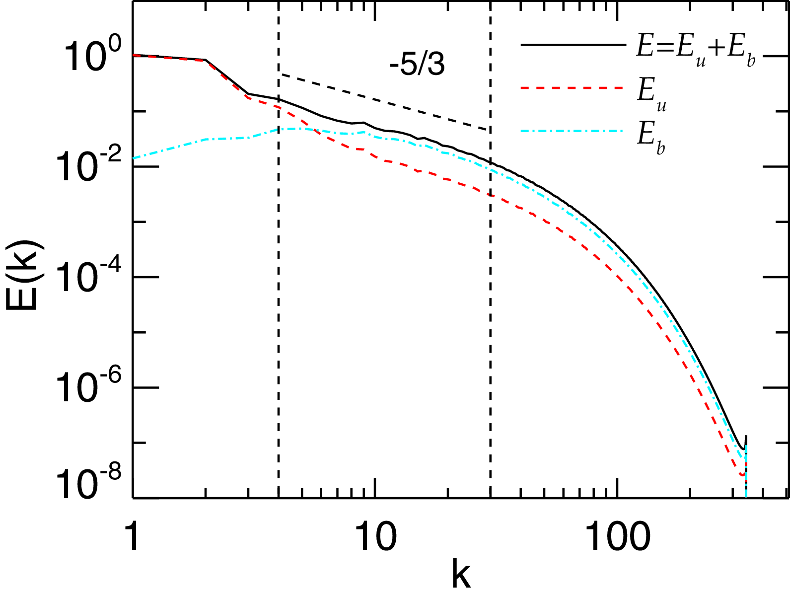
The energy spectra are shown in figure 1 and the
 $k^{-5/3}$
is also plotted for reference. One can see that both kinetic and magnetic energies show a scaling close to
 $k^{-5/3}$
over a range of wavenumbers (
 $4\leqslant k \leqslant 30$
), which are roughly viewed as the inertial range.
Kinetic
 $E_u(k)$
, magnetic
 $E_b(k)$
and total energy
 $E(k)=E_u(k)+E_b(k)$
spectra. The
 $k^{-5/3}$
scaling is plotted for reference. The two dashed lines mark the inertial range over which the spectra exhibit a power law close to
 $k^{-5/3}$
.

Spatial distributions of (a) point-wise dissipation rate
 $\varepsilon$
, (b) the square of current density
 $j^2$
and (c) the square of vorticity density
 $\omega ^2$
for one time frame of the MHD simulation.

3. Results
3.1. Dissipation rate
We calculated the point-wise value of dissipation rate
 $\varepsilon (\boldsymbol{x})$
as (1.12) from one time frame of the MHD simulation data, and compared it in figure 2 with the spatial distributions of the current density
 $j^2$
and the vorticity density
 $\omega ^2$
. As shown in figure 2, the dissipation rate has intermittent structures similar to those of the current and vorticity fields. This indicates that these intermittent structures are indeed strongly correlated. In many hydrodynamic turbulent flows, the dominant structures are found to be tubelike, such as vortex tubes with concentrated enstrophy, whereas sheet-like structures between these tubes with intense strain rate are regions of dissipation. It is therefore expected that an intense dissipation rate is strongly correlated with a large strain rate, rather than a large vorticity. This is confirmed in hydrodynamic turbulence away from walls (Jiménez et al. Reference Jiménez, Wray, Saffman and Rogallo1993; Blackburn, Mansour & Cantwell Reference Blackburn, Mansour and Cantwell1996). Unlike the hydrodynamic turbulence, many visualisations of MHD turbulence exhibit a frequently occurring class of sheet-like rather than tube-like structures (Mininni & Pouquet Reference Mininni and Pouquet2009; Dallas & Alexakis Reference Dallas and Alexakis2013), which is also reported in figure 2. This could be attributed to the strong correlation between the intense strain rate and vorticity (Yang et al. Reference Yang, Matthaeus, Parashar, Haggerty, Roytershteyn, Daughton, Wan, Shi and Chen2017; Chasapis et al. Reference Chasapis2018; Bandyopadhyay et al. Reference Bandyopadhyay2020). Since the strain rate is in direct association with the viscous dissipation, this is suggestive that the viscous dissipation and the vorticity are also strongly correlated, which is consistent with the similar patterns of
 $\varepsilon (\boldsymbol{x})$
and
 $\omega ^2$
in figure 2. Previous works (Dallas & Alexakis Reference Dallas and Alexakis2013; Yang et al. Reference Yang, Matthaeus, Parashar, Haggerty, Roytershteyn, Daughton, Wan, Shi and Chen2017; Chasapis et al. Reference Chasapis2018; Bandyopadhyay et al. Reference Bandyopadhyay2020) report a weak point-wise correlation between current density and velocity gradient, which may seem at first to be in conflict with the finding of figure 2. However, one may follow previous works (Matthaeus Reference Matthaeus1982; Parashar & Matthaeus Reference Parashar and Matthaeus2016) where vorticity structures tend to form on the flanks of strong current structures, such that the intense vorticity does not collapse exactly with, but locates in the vicinity of the strong current. In this sense, the dissipation rate
 $\varepsilon (\boldsymbol{x})$
, the current density
 $j^2$
and the vorticity density
 $\omega ^2$
in figure 2 reveal greatly similar patterns.
Recall that intermittency is not accounted for in the original Kolmogorov similarity hypothesis (Kolmogorov Reference Kolmogorov1941) and the refined similarity hypothesis (RSH) (Kolmogorov Reference Kolmogorov1962) is the first attempt to include its effects. After that, a large amount of work has been devoted to validating the RSH in hydrodynamic turbulence. They also found that the distribution of
 $\varepsilon _r$
in the inertial range follows a log-normal distribution proposed by Kolmogorov (Reference Kolmogorov1962). In the recent work by Jiang et al. (Reference Jiang, Yang, Ye, Li, Wang, Oughton, Matthaeus and Wan2026), the statistics of the locally averaged dissipation rate have been investigated in MHD turbulence, which suggests that
 $\varepsilon _r$
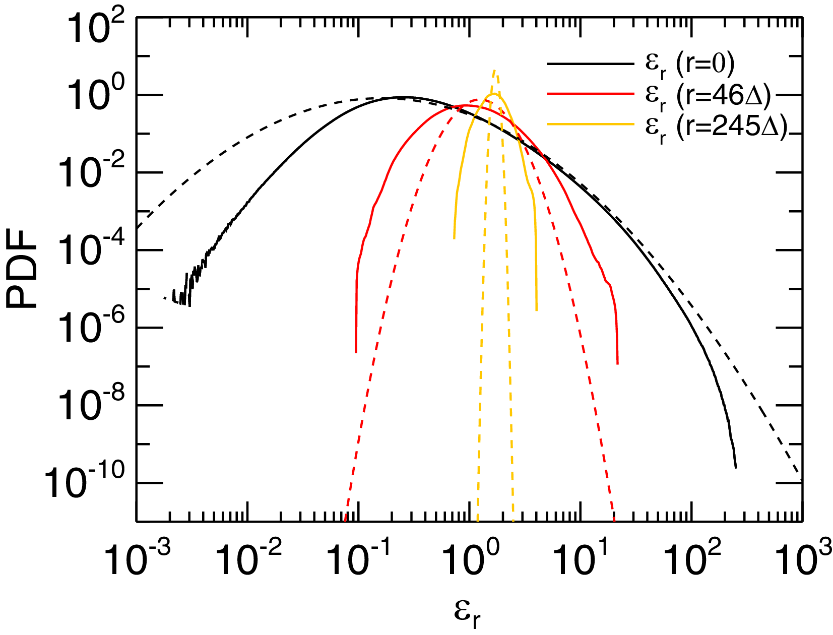
might not be log-normally distributed, also seen in figure 3. We calculated the probability density functions (p.d.f.s) of locally averaged dissipation rate
 $\varepsilon _r$
at different scales
 $r$
, as implemented in (1.14), and show them in figure 3. Three representative scales (
 $r=0$
at the dissipation range,
 $r=46\Delta$
at the inertial range and
 $r=245\Delta$
at the energy-containing range) are shown. Note that
 $\varepsilon _r$
when
 $r=0$
corresponds to the pointwise dissipation rate
 $\varepsilon$
, i.e.
 $\varepsilon _{r=0}=\varepsilon$
. The p.d.f.s of
 $\varepsilon _r$
have extended tails for the smallest
 $r$
, consistent with the stronger intermittency at smaller scales seen in figure 2. When the scale increases to the energy-containing range, see
 $r=245\Delta$
, the tails are suppressed and the intensive regions are smoothed.
Probability density functions of locally averaged dissipation rate
 $\varepsilon _r$
at
 $r = 0$
(black solid line, at the dissipation range),
 $r = 46\Delta$
(red solid line, at the inertial range),
 $r = 245\Delta$
(orange solid line, at the energy-containing range). We also provide p.d.f.s of log-normal distributions (black, red, and orange dashed lines) based on the p.d.f.s of
 $\varepsilon _r$
for comparison. The means of log-normal distributions are –0.14 (black line), 0.37 (red line) and 0.54 (orange line), while the standard deviations are 1.3 (black line), 0.40 (red line) and 0.050 (orange line). Note that the means and standard deviations are of the log-transformed variables.

The spatial distributions of
 $\varepsilon _r$
from one time frame of the simulation for different scales are shown in figure 4. As one can see, the extremely intense dissipation localised in very small regions is smoothed when local averaging is applied. As expected, figure 4 also shows that dissipation is more prominent at the smallest scales with the most intense values and its influence will decrease with less extreme values as the scale increases (Yordanova et al. Reference Yordanova, Vörös, Sorriso-Valvo, Dimmock and Kilpua2021).
Spatial distributions of locally averaged dissipation rate
 $\varepsilon _r$
at (a)
 $r_0 = 0$
, (b)
 $r_2 = 46\Delta$
(at the inertial range), (c)
 $r_3 = 245\Delta \sim L_{\!f}$
(at the energy-containing range), for one time frame of the MHD simulation, where
 $\varDelta$
is the grid cell size and
 $L_{\!f}$
is the correlation length scale.

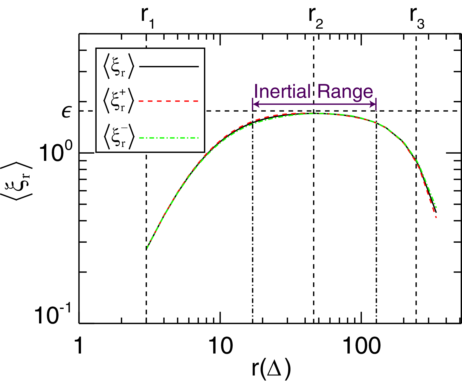
Global averages of local energy transfer (LET) rate
 $\langle \xi _r \rangle$
and
 $\langle \xi _r^\pm \rangle$
across scales
 $r$
. The mean dissipation rate
 $\epsilon$
is plotted for reference. The vertical dashed lines mark three representative scales
 $r_1=3\Delta$
,
 $r_2=46\Delta$
and
 $r_3=245\Delta$
in the dissipation range, inertial range and energy-containing range, respectively. The inertial range identified via
 $\langle \xi _r \rangle \geqslant 0.85 \epsilon$
is also marked.

3.2. Local energy transfer (LET) rate
The unaveraged third-order mixed structure function has been used to identify the local energy transfer (Sorriso-Valvo et al. Reference Sorriso-Valvo, Marino, Lijoi, Perri and Carbone2015, Reference Sorriso-Valvo, Carbone, Perri, Greco, Marino and Bruno2018a
,
Reference Sorriso-Valvo, Perrone, Pezzi, Valentini, Servidio, Zouganelis and Veltrib
; Yang et al. Reference Yang, Wan, Matthaeus, Sorriso-Valvo, Parashar, Lu, Shi and Chen2018; Matthaeus et al. Reference Matthaeus, Yang, Wan, Parashar, Bandyopadhyay, Chasapis, Pezzi and Valentini2020) and the local energy transfer (LET) rate across scale
 $r$
is estimated through
 $\xi ^\pm _r$
for Elsässer fields in (1.6).
We first calculate the global averages of
 $\xi _r$
and
 $\xi ^\pm _r$
at different scales
 $r$
, as shown in figure 5. One can see that the values are minimal at small scales (
 $r_1 = 3\Delta$
) and gradually increase with
 $r$
, reaching a peak in the inertial range at
 $r_2 = 46\Delta$
. After that,
 $\langle \xi _r \rangle$
and
 $\langle \xi _r^\pm \rangle$
gradually decrease until the largest scale. The plateau (or peak) of
 $\langle \xi _r \rangle$
deviates slightly from the mean dissipation rate
 $\varepsilon$
. In a well-separated inertial range, the third-order law in (1.2) can be satisfied to a great degree and
 $\langle \xi _r \rangle$
can reach
 $\varepsilon$
therein. It is well known that the inertial range width increases with the Taylor Reynolds number
 $Re_{\lambda }$
. A recent study in MHD turbulence suggests that this value should exceed 1500 to have an inertial range wider than two decades (Ye et al. Reference Ye, Yang, Jiang, Li, Wan, Shi and Oughton2025). One can therefore expect that for simulations with longer well-separated inertial ranges, the plateau of
 $\langle \xi _r \rangle$
will be closer to
 $\epsilon$
. Assuming homogeneity and isotropy, we can also define the inertial range as a set of scales over which the third-order law in (1.2) is satisfied to an accuracy, and here we use
 $\langle \xi _r \rangle \geqslant 0.85 \epsilon$
. The identified inertial range is
 $17\Delta \leqslant r \leqslant 128\Delta$
. One may recall that the inertial range identified from the energy spectra in figure 1 is roughly
 $17 - 128 \Delta$
(
 $r=\pi /k$
), which is equal to that based on the third-order structure function shown in figure 5. This is consistent with the hydrodynamic and magnetohydrodynamic findings of Antonia et al. (Reference Antonia, Tang, Djenidi and Zhou2019), Ye et al. (Reference Ye, Yang, Jiang, Li, Wan, Shi and Oughton2025).
Figure 6 shows the spatial distributions of
 $\xi _r$
at scales
 $r_1$
,
 $r_2$
and
 $r_3$
in the dissipation range, inertial range and energy-containing range, respectively. Again,
 $\xi _r$
at different lags have similar spatial distributions. They are the most intense at
 $r_2$
in the inertial range and are relatively weak at small scale
 $r_1$
and large scale
 $r_3$
.
Contour maps of LET
 $\xi _r$
at
 $r_1 = 3\Delta$
,
 $r_2 = 46\Delta$
and
 $r_3 = 245\Delta$
for one time frame of the MHD simulation.

Figure 6. Long description
Panel A: A heat map with a color scale ranging from blue to red, representing values from -1.0 to 1.0. The x-axis is labeled ‘x(Δ)’ and ranges from 0 to 1000. The y-axis is labeled ‘y(Δ)’ and ranges from 0 to 1000. The map shows a complex pattern of swirling colors, indicating varying data intensities. Panel B: A heat map with a color scale ranging from blue to red, representing values from -10 to 10. The x-axis is labeled ‘x(Δ)’ and ranges from 0 to 1000. The y-axis is labeled ‘y(Δ)’ and ranges from 0 to 1000. The map displays intricate swirling patterns with areas of high and low intensity. Panel C: A heat map with a color scale ranging from blue to red, representing values from -10 to 10. The x-axis is labeled ‘x(Δ)’ and ranges from 0 to 1000. The y-axis is labeled ‘y(Δ)’ and ranges from 0 to 1000. The map features a mix of red, blue, and yellow regions, indicating diverse data intensities.
3.3. Scale-filtered energy flux
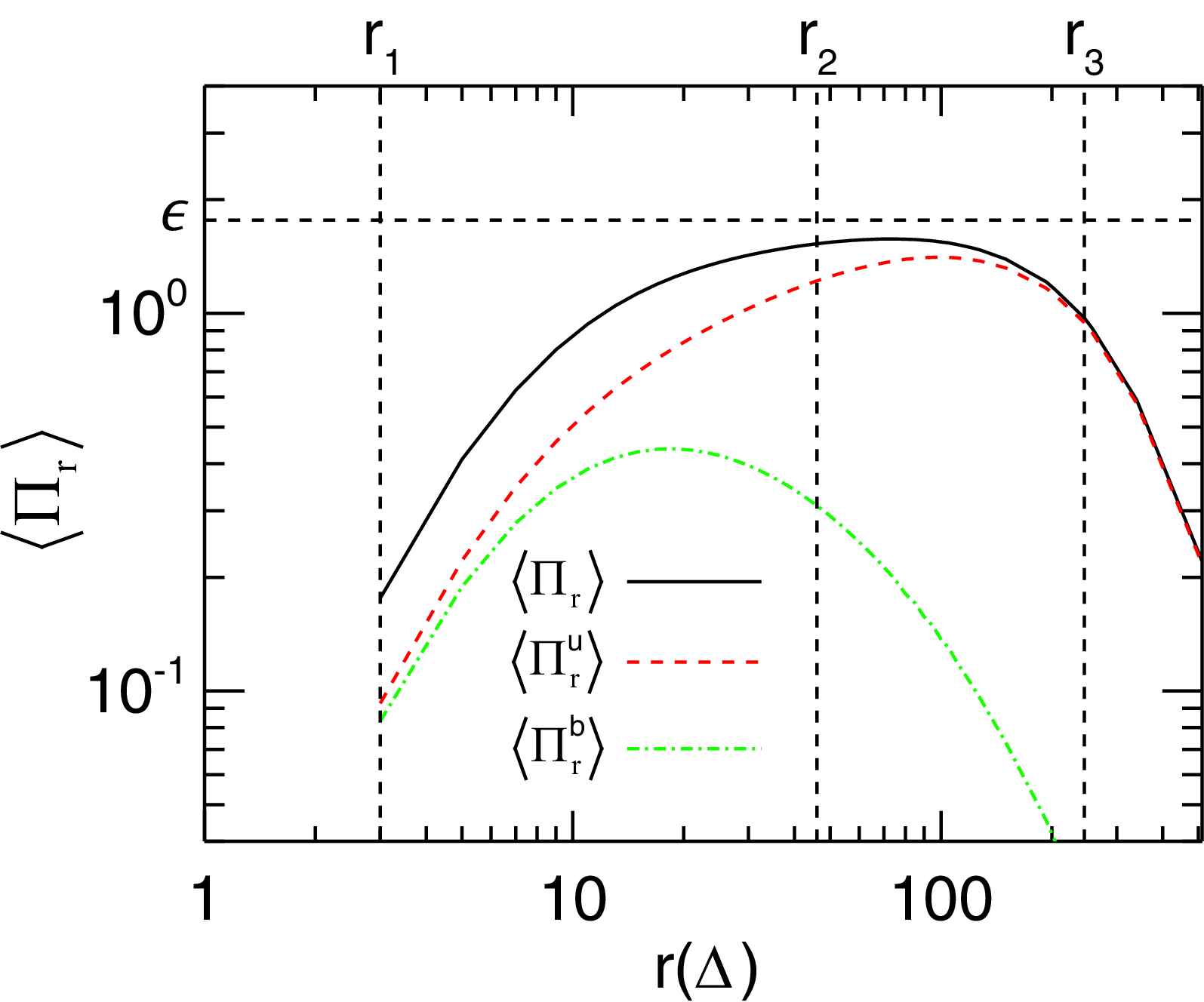
The global average values of
 $\varPi ^u_r$
,
 $\varPi ^b_r$
and
 $\varPi _r = \varPi ^u_r + \varPi ^b_r$
defined in (1.10) at different scales
 $r$
are shown in figure 7. The same tendency as in figure 5 is also exhibited, that is, the values are minimal at small scales (
 $r_1 = 3\Delta$
) and gradually increase with
 $r$
, reaching peak values in the inertial range
 $17 {-} 128 \Delta$
. After that, they gradually decrease as approaching the large correlation lengthscale. The plateau of
 $\langle \varPi _r \rangle$
is close to (though not exactly equal to) the mean dissipation rate
 $\epsilon$
, which can be reasoned in the same way as the LET shown in figure 5. The contour maps of scale-filtered energy flux
 $\varPi _r$
at different scales in figure 8 again exhibit similar patterns. They are most intense in the inertial range at
 $r_2$
and are quite weak at small scale
 $r_1$
and large scale
 $r_3$
.
Space-averaged scale-filtered energy flux
 $\varPi _r$
, kinetic energy flux
 $\varPi ^u_r$
and magnetic energy flux
 $\varPi ^b_r$
as a function of separation length
 $r$
. The mean dissipation rate
 $\epsilon$
is plotted for reference.

Contour maps of scale-filtered energy flux
 $\varPi _r$
at scales
 $r_1 = 3\Delta$
,
 $r_2 = 46\Delta$
and
 $r_3 = 245\Delta$
, for one time frame of the simulation.

3.4. Correlations
As discussed, the LET
 $\xi _r$
and the scale-filtered energy flux
 $\varPi _r$
dominate at the inertial range, while the dissipation
 $\varepsilon$
mainly occurs at the dissipation scales. Nevertheless, their global averages are nearly equal, as shown in figures 5 and 7. This is expected when the cascade scenario over the inertial range is established. Therefore, in the absence of viscous and ohmic dissipation, such as in the weakly collisional/collisionless plasmas, the energy dissipation rate could in principle be estimated by either
 $\langle \xi _{r}\rangle$
or
 $\langle \varPi _{r}\rangle$
at the inertial range. In addition to the association between the LET
 $\xi _r$
, the scale-filtered energy flux
 $\varPi _r$
and the dissipation
 $\varepsilon$
in the global sense, their spatial distributions also exhibit similar patterns, see for example, figures 4, 6, and 8. The intense
 $\xi _r$
,
 $\varPi _r$
and
 $\varepsilon$
are nearly colocated by naked eyes, which also resembles the distribution of current sheets in our case.
However,
 $\varPi _r$
,
 $\xi _{r}$
and
 $\varepsilon$
are derived from different approaches. Here,
 $\varepsilon$
is positive definite while
 $\varPi _r$
and
 $\xi _{r}$
could be positive (implying locally forward cascade) or negative (implying locally inverse cascade). We anticipate that they are not exactly co-located with each other. This is supported by the joint probability density functions of
 $\varPi _{r_2}$
,
 $\xi _{r_2}$
and
 $\varepsilon$
(not shown here), which are widely spreading and do not exhibit a visible correlation. A scale-dependent, cross-correlation function that has been frequently used in previous research (Parashar & Matthaeus Reference Parashar and Matthaeus2016; Yang et al. Reference Yang, Wan, Matthaeus, Sorriso-Valvo, Parashar, Lu, Shi and Chen2018) could describe this complex spatial arrangement:
 \begin{align} R(f,g,\ell ) = \frac {\langle f'(\boldsymbol{x} + \boldsymbol{\ell }) g'(\boldsymbol{x}) \rangle }{\langle f'(\boldsymbol{x}) g'(\boldsymbol{x}) \rangle }, \end{align}
where
 $f$
and
 $g$
are the fields,
 $f'=f-\langle f \rangle$
and
 $g'=g-\langle g \rangle$
are the fluctuations,
 $\langle \boldsymbol{\cdot }\rangle$
denotes an average over the entire spatial domain, and
 $R(f,g,\ell )$
is the correlation between
 $f$
and
 $g$
at the displacement scale
 $\ell$
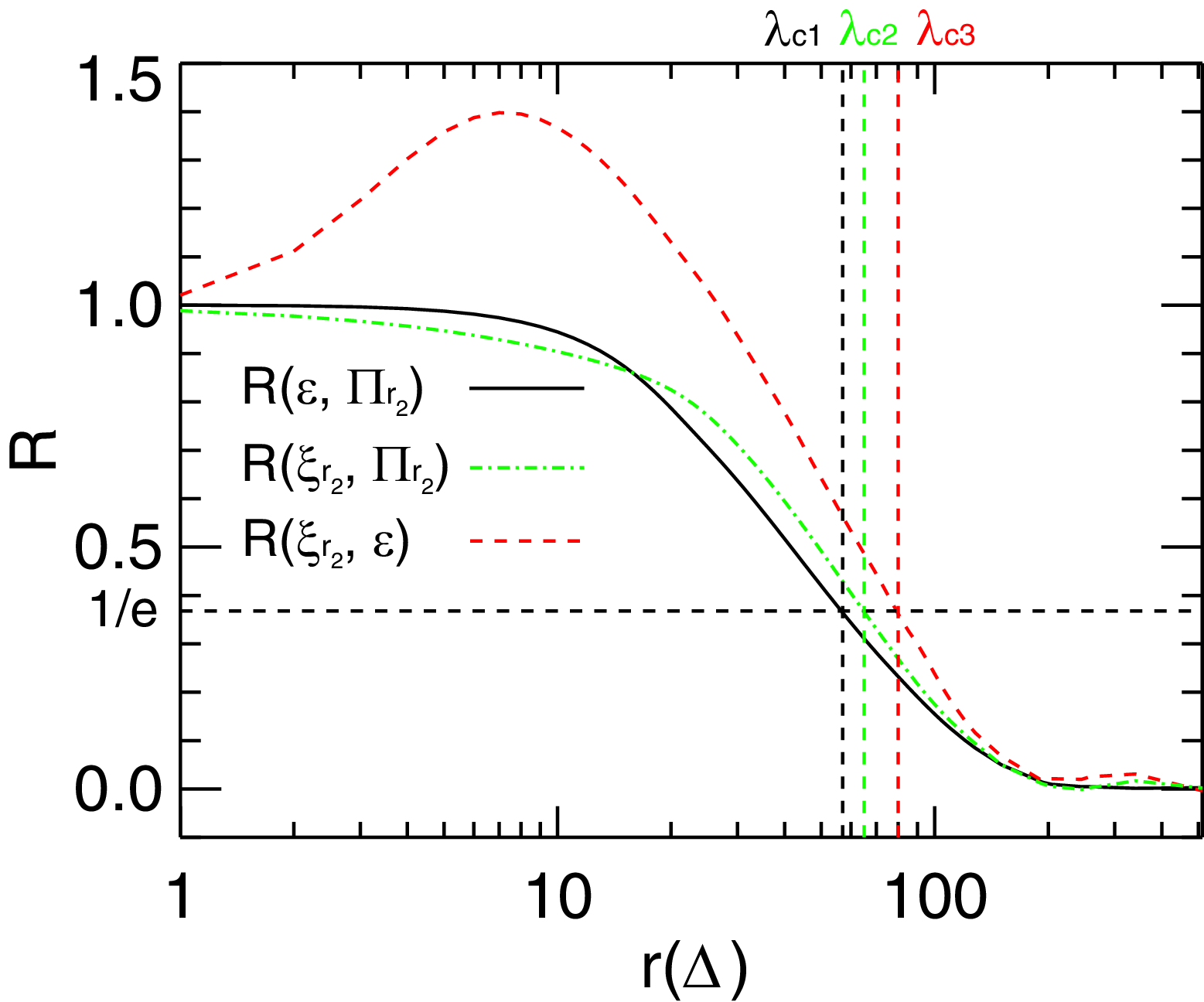
. We plot the cross-correlation functions
 $R(\varepsilon ,\varPi _{r_2},\ell )$
,
 $R(\xi _{r_2},\varPi _{r_2},\ell )$
and
 $R(\xi _{r_2},\varepsilon ,\ell )$
in figure 9. We can expect that when
 $\ell =0$
,
 $R=1$
, and as
 $\ell \rightarrow \infty$
,
 $R \rightarrow 0$
, as also shown in figure 9. However, the cross-correlation
 $R$
is not necessarily monotonically decreasing. Note that the correlation curve of
 $R(\xi _{r_2},\varepsilon ,\ell )$
has a peak value (
 $\gt 1$
) at
 $\ell = 7\Delta$
, indicating that the dissipation rate and the LET have the strongest correlation at a small displacement. The excess of unity in figure 9 supports that the intensive
 $\varepsilon$
and
 $\xi _{r2}$
are not exactly collocated, but occur at locations with a certain displacement. From the correlation function, we can calculate the correlation length
 $\lambda _c$
by
 $R|_{r = \lambda _c} = 1/\text{e}$
, a measure of the scales over which the fields are appreciably correlated. The correlation lengths of
 $R(\varepsilon ,\varPi _{r_2},\ell )$
,
 $R(\xi _{r_2},\varPi _{r_2},\ell )$
and
 $R(\xi _{r_2},\varepsilon ,\ell )$
are listed in figure 9. The inertial range identified from the energy spectra in figure 1 is roughly
 $17{-} 128 \Delta$
(
 $\ell =\pi /k$
). Therefore, the correlation lengths in figure 9 are in the inertial range and the correlation length of
 $R(\varepsilon ,\varPi _{r_2},\ell )$
is the smallest. The LET, the scale-filtered energy flux and the dissipation rate, although not exactly colocated, are concentrated in proximity to each other. This also indicates that the spatial distributions of LET and the scale-filtered energy flux can provide a reliable picture of the energy transfer and dissipation in turbulence.
Two-point cross-correlation functions of LET, dissipation rate and scale-filtered energy flux.
 $\lambda _{c1}=57\Delta$
,
 $\lambda _{c2}=65\Delta$
and
 $\lambda _{c3}=80\Delta$
are the correlation length of
 $R(\varepsilon ,\varPi _{r_2},\ell )$
,
 $R(\xi _{r_2},\varPi _{r_2},\ell )$
and
 $R(\xi _{r_2},\varepsilon ,\ell )$
, respectively.

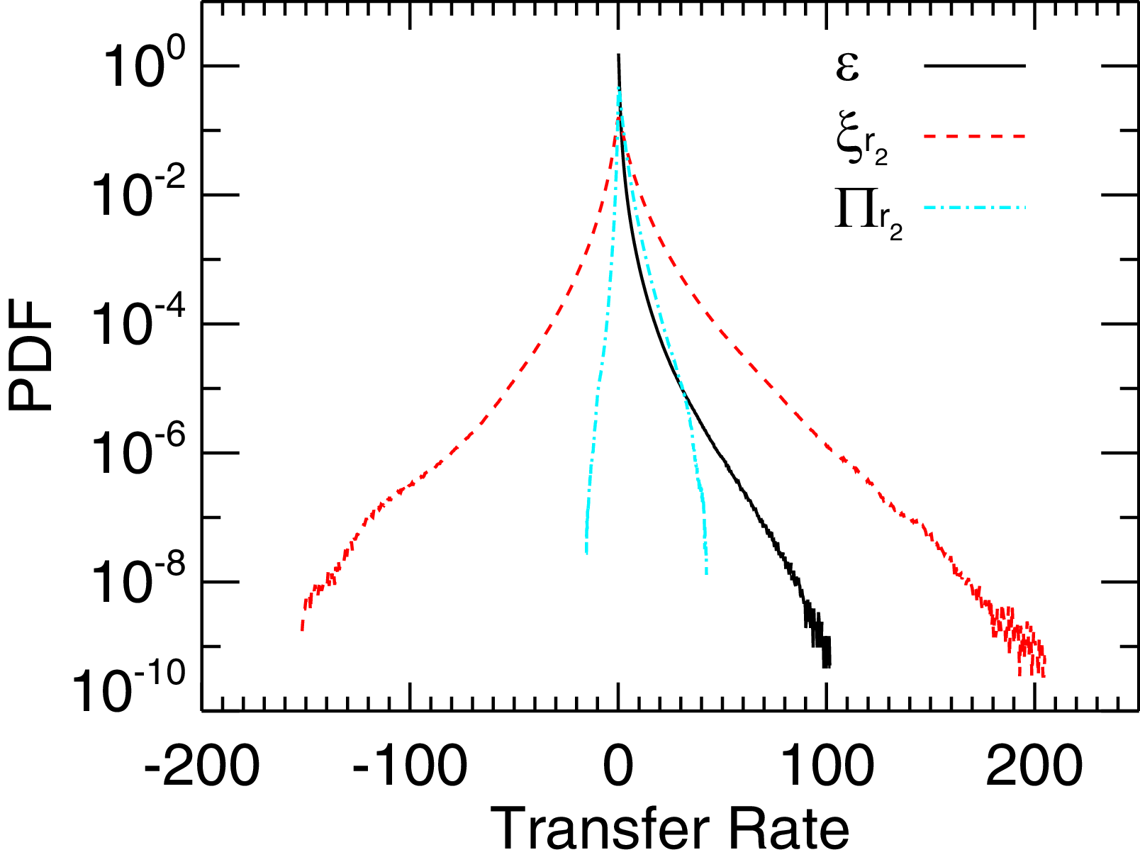
Probability density functions of dissipation rate
 $\varepsilon$
, LET
 $\xi _{r_2}$
and scale-filtered flux
 $\varPi _{r_2}$
.

To further examine the association between the three diagnostics, we plot the p.d.f.s of the dissipation rate
 $\varepsilon$
, LET
 $\xi _{r_2}$
and the scale-filtered flux
 $\varPi _{r_2}$
in figure 10. One can observe that the p.d.f. of the scale-filtered flux
 $\varPi _{r_2}$
is much closer to that of the dissipation rate
 $\varepsilon$
, while the p.d.f. of LET
 $\xi _{r_2}$
deviates significantly from the other two diagnostics. This reconciles with the theoretical rationales of LET
 $\xi _{r}$
and the scale-filtered flux
 $\varPi _{r}$
. Recall that the scale-filtered flux is rigorously derived from the low-pass filtered MHD equations, as shown in (1.10). In this sense, one could interpret the LET as an indicator of very local contribution to energy transfer, which often appears as bipolar oscillations that, when averaged over a small volume (Manzini et al. Reference Manzini, Sahraoui, Califano and Ferrand2022), strongly cancel each other, resulting in the net local energy transfer. Taking LET
 $\xi _{r_2}$
as an example, we locally average
 $\xi _{r_2}$
over a cube of size
 $\ell$
, same as the procedure in (1.14), and obtain
 $\overline {(\xi _{r_2})}_\ell$
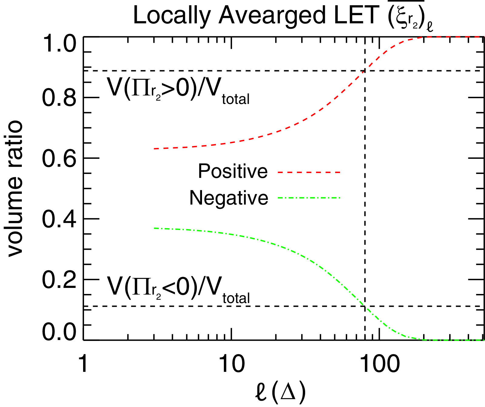
. The volume fractions of positive and negative values of the locally averaged
 $\overline {(\xi _{r_2})}_\ell$
as a function of averaging scale
 $\ell$
are shown in figure 11, where one can see that local averaging eliminates the extreme values of LET
 $\xi _{r_2}$
and the positive values dominate over the negative ones. Also shown are the volume fractions of positive and negative values of the scale-filtered flux
 $\varPi _{r_2}$
. Note that at
 $\ell \sim 80\Delta$
, the ratio of
 $\overline {(\xi _{r_2})}_\ell$
is equal to that of
 $\varPi _{r_2}$
. One can therefore expect that the p.d.f. of the locally averaged
 $\overline {(\xi _{r_2})}_\ell$
at
 $\ell \sim 80\Delta$
will be more analogous to that of the scale-filtered flux
 $\varPi _{r_2}$
. That is, the energy transfer quantified by the local fluctuations of LET is much larger than the actual energy being transferred across scales, and necessary coarse-graining is required to eliminate the strong fluctuations and refine the estimate of LET.
Volume fractions of positive and negative values of the locally averaged
 $\overline {(\xi _{r_2})}_\ell$
over an averaged volume of size
 $\ell$
. Also shown are the volume fractions of positive and negative values of the scale-filtered flux
 $\varPi _{r_2}$
. Note that at
 $\ell \sim 80\Delta$
, the ratio of
 $\overline {(\xi _{r_2})}_\ell$
is equal to that of
 $\varPi _{r_2}$
.

When LET and scale-filtered flux are computed at a very small scale
 $r_1$
, similar analyses, including the cross-correlation function, the p.d.f. and the joint p.d.f., are conducted. The corresponding correlation length is
 $\sim 8\Delta$
, which lies in the dissipation range. The p.d.f.s shown in figure 12(a) resemble each other, and the joint p.d.f. of
 $\varPi _{r_1}$
and
 $\varepsilon$
in figure 12(b) shows a strong correlation (Pearson correlation coefficient
 $\sim 0.78$
). Recent results in MHD turbulence (Alexakis & Chibbaro Reference Alexakis and Chibbaro2022) demonstrate a correlation between the local energy flux and the gradients of the involved fields, which is consistent with the correlation we are showing here. The correlation lengths among LET
 $\xi _{r_1}$
,
 $\varPi _{r_1}$
and
 $\varepsilon$
are shorter and a more correlated joint p.d.f. at
 $r_1$
is also shown in figure 12, with respect to the same analysis at
 $r_2$
. The results seem to be in conflict with previous evidence that the LET and scale-filtered flux work better in the inertial range and are not great proxies of energy transfer at the dissipation range. However, this indicates that, on average, they are no longer a good estimate of the global dissipation rate at very small scales, but locally, they highlight similar small-scale structures showing the more intense values.
(a) Probability density functions of dissipation rate
 $\varepsilon$
, LET
 $\xi _{r_1}$
and the scale-filtered flux
 $\varPi _{r_1}$
. (b) Joint probability density functions of dissipation rate
 $\varepsilon$
and the scale-filtered flux
 $\varPi _{r_1}$
.

4. Conclusion and discussion
In this work, we assess the local energy transfer through three diagnostics: the dissipation rate, the local energy transfer (LET) rate and the scale-filtered energy flux. We first derive them from the MHD equations or from assumptions, in detail, to show that they can, in theory, quantify energy transfer in turbulence. Among them, the dissipation rate, if accessible, is the most accurate measure of dissipation. Still, it requires viscosity, resistivity, and velocity and magnetic field gradients, which are available only in numerical simulations. The scale-filtered energy flux is also rigorous but requires adequate data to compute the sub-grid-scale stress and gradients. The LET is derived from assumptions, but requires far fewer data, making it the most widely used in real space plasmas.
Our analyses of their values and spatial distributions across scales support that the impact of the dissipation rate shows the most intense fluctuations at small scales, while the influence of LET and the scale-filtered energy flux peaks at the inertial range. The accuracy of the three in capturing energy transfer rates diminishes as the scale approaches the energy-containing range. We compared the spatial distributions of the three at their peak intensity to show their correlations. Their spatial distributions exhibit similar patterns, but are not exactly co-located. To analyse this complex spatial arrangement, we apply the scale-dependent cross-correlation function. Their respective correlation lengths over which the three are appreciably correlated lie in the inertial range. Even though both LET and the scale-filtered energy flux can identify local sites with intense energy transfer, the scale-filtered energy flux provides a more accurate estimate of energy transfer at the inertial range.
Our results support the ‘regional correlation’ (Yang et al. Reference Yang, Wan, Matthaeus, Sorriso-Valvo, Parashar, Lu, Shi and Chen2018; Matthaeus et al. Reference Matthaeus, Yang, Wan, Parashar, Bandyopadhyay, Chasapis, Pezzi and Valentini2020) that has been commonly observed before. That is, the energy transfer channels at different scales, though not exactly colocated, are in the vicinity of each other. Wan et al. (Reference Wan, Xiao, Meneveau, Eyink and Chen2010) and Cardesa, Vela-Martín & Jiménez (Reference Cardesa, Vela-Martín and Jiménez2017) investigated the Lagrangian energy cascade in hydrodynamic turbulence, and found that the correlation between the dissipation rate
 $\varepsilon$
and the scale-filtered flux
 $\varPi _r$
is scale-dependent. Some time must be allowed for energy to transfer from the inertial range to the dissipation scale, meaning that the energy dissipation at
 $(\boldsymbol{x},t)$
may be caused by the energy flux at
 $(\boldsymbol{x},t-\delta t)$
. In this sense, there is no direct causality between
 $\varepsilon (\boldsymbol{x},t)$
and
 $\varPi (\boldsymbol{x},t)$
, leading to the lack of point-to-point correlation between the spatial distribution of
 $\varepsilon$
and
 $\varPi _r$
. Wan et al. (Reference Wan, Xiao, Meneveau, Eyink and Chen2010) have also shown that the time required for the energy to transfer from a smaller scale
 $r$
to the dissipation range is shorter, so the spatial correlation between
 $\varPi _r$
with a smaller filter scale and
 $\varepsilon$
is stronger, just like
 $\varPi _{r_1}$
and
 $\varepsilon$
in figure 12(b). As guided by Wan et al. (Reference Wan, Xiao, Meneveau, Eyink and Chen2010), future work will be done in this direction to explain the ‘regional correlation’ in MHD and plasma turbulence. Another important aspect in assessing the causality of energy transfer and cross-scale coupling across different regimes (inertial MHD, dissipative and kinetic) is the possibility of dual cascades in plasmas, whereby injected energy is transferred simultaneously to smaller and larger scales. Such behaviour has been observed in kinetic plasmas (Foldes et al. Reference Foldes, Cerri, Marino and Camporeale2024) and in the solar wind at magnetohydrodynamic scales (Marino & Xie Reference Marino and Xie2025).
We should also keep in mind the caveat about the filtering strategy. It has been suggested that a smooth filter (e.g. Gaussian filter) could be more suitable for analysing multi-scale energy transfer and local properties than a sharp filter (e.g. the boxcar filter used in our work) (Germano Reference Germano1992; Aluie & Eyink Reference Aluie and Eyink2009; Eyink & Aluie Reference Eyink and Aluie2009). However, Domaradzki & Carati (Reference Domaradzki and Carati2007a , Reference Domaradzki and Caratib ), Domaradzki, Teaca & Carati (Reference Domaradzki, Teaca and Carati2009) and Buzzicotti et al. (Reference Buzzicotti, Linkmann, Aluie, Biferale, Brasseur and Meneveau2018) have shown that these two kinds of filter are qualitatively consistent with each other when describing energy transfer functions, and the energy flux obtained with a sharp filter is scale-localised, as with a smooth filter. Here, we used a boxcar filter for simplicity and it also represents a simple choice when applied to single-spacecraft measurements. We anticipate that the qualitative conclusions in our work still hold when using smooth filters. To show possible effects of the filtering type, an example of the scale-filtered fluxes by using the Gaussian filter and the boxcar filter is shown in figure 13, where one can see that the overall patterns are quite similar, even though the Gaussian-filtered one exhibits finer structures. We can therefore affirm that the qualitative conclusions in our work are essentially independent of the filter choice.
Scale-filtered energy flux
 $\varPi _r$
at scale
 $r_2 = 46\Delta$
calculated with (a) boxcar filter and (b) Gaussian filter.

Note that we focus on the homogeneous isotropic case and it is necessary to extend our work to more realistic cases with anisotropy, which are quite typical in real space plasmas (Horbury, Wicks & Chen Reference Horbury, Wicks and Chen2012; Oughton et al. Reference Oughton, Matthaeus, Wan and Osman2015). It has been recognised that the energy transfer varies systematically over the direction relative to the mean magnetic field (Verdini et al. Reference Verdini, Grappin, Hellinger, Landi and Müller2015; Schekochihin Reference Schekochihin2022; Jiang et al. Reference Jiang, Li, Yang, Zhou, Matthaeus and Wan2023). A general picture is that the energy transfer along the mean magnetic field direction will be suppressed. Several methods to quantify energy transfer rate have been employed to account for the anisotropic effect, including the hybrid formulation (e.g. one-dimensional plus two-dimensional) (Stawarz et al. Reference Stawarz, Smith, Vasquez, Forman and MacBride2009; Coburn et al. Reference Coburn, Forman, Smith, Vasquez and Stawarz2015; Verdini et al. Reference Verdini, Grappin, Hellinger, Landi and Müller2015; Andrés et al. Reference Andrés, Sahraoui, Huang, Hadid and Galtier2022), the direction-averaging method (Taylor, Kurien & Eyink Reference Taylor, Kurien and Eyink2003; Wang et al. Reference Wang, Chhiber, Adhikari, Yang, Bandyopadhyay, Shay, Oughton, Matthaeus and Cuesta2022; Jiang et al. Reference Jiang, Li, Yang, Zhou, Matthaeus and Wan2023; Gao et al. Reference Gao, Yang, Pecora, Jiang, Klein, Chasapis, Stawarz and Matthaeus2026) and the lag polyhedral derivative ensemble (LPDE) method (Pecora et al. Reference Pecora2023a,b
; Gao et al. Reference Gao, Yang, Pecora, Jiang, Klein, Chasapis, Stawarz and Matthaeus2026). To account for the anisotropic effect on the three diagnostics we are studying here, more refined analyses should be done. For example, the LET
 $\xi _r$
should be calculated along varying separation vector
 $\boldsymbol{r}$
directions and an anisotropic scale filter should be used to obtain
 $\varPi _r$
. Instead of using the isotropic spherical/cubic average to obtain
 $\varepsilon _r$
, an anisotropic average, such as elliptical or line average, could be more appropriate. Meanwhile, the external forcing we are employing here does not introduce anisotropy, but its possible effects on energy cascade behaviour warrant more investigation, and one may refer to the works of Yang et al. (Reference Yang, Linkmann, Biferale and Wan2021); Foldes et al. (Reference Foldes, Marino, Cerri and Camporeale2025b
), Jiang et al. (Reference Jiang, Yang, Ye, Li, Wang, Oughton, Matthaeus and Wan2026) and Li et al. (Reference Li, Yang, Matthaeus, Jiang, Oughton, Wan and Chen2026).
Our current research has only covered the scale from the dissipation range to the inertial range. It has been noted that additional energy-transfer channels must be considered at scales smaller than the dissipation range, i.e. the kinetic scale. Therefore, our future research will focus on energy transfer at the kinetic scale, in which the dissipation rate
 $\varepsilon$
is unavailable and could instead be quantified by the electromagnetic work
 $\boldsymbol{j}\boldsymbol{\cdot }\boldsymbol{E}$
(Zenitani et al. Reference Zenitani, Hesse, Klimas and Kuznetsova2011) and the pressure-strain interaction
 $-(\boldsymbol{P}\boldsymbol{\cdot }\boldsymbol{\nabla })\boldsymbol{\cdot }\boldsymbol{u}$
(Yang et al. Reference Yang, Matthaeus, Parashar, Haggerty, Roytershteyn, Daughton, Wan, Shi and Chen2017). Meanwhile, it is worthwhile to conduct similar analyses by using in situ spacecraft measurements, where kinetic effects on energy transfer need to be taken into account. We suspect that in kinetic plasmas, an inertial range cascade process may be similar to what is seen in MHD, and the results for the LET and the scale-filtered flux in kinetic plasmas could be analogous to those reported here. However, a reliable measurement of the scale-filtered energy flux
 $\varPi _r$
and the pressure-strain interaction
 $-(\boldsymbol{P}\boldsymbol{\cdot }\boldsymbol{\nabla })\boldsymbol{\cdot }\boldsymbol{u}$
requires the calculation of derivatives using curlometer-like techniques (Paschmann et al. Reference Paschmann and Daly2008), which requires at least 4 spacecraft, so principally multi-spacecraft observations are required. One may also resort to possible one-dimensional surrogates. For example, Adhikari et al. (Reference Adhikari, Cassak, Barbhuiya, Shay, Chasapis, Yang and Matthaeus2025) proposed an approximation of the pressure-strain interaction for magnetic reconnection in the strong guide field limit.
Acknowledgements
The authors thank Minping Wan for helpful discussions.
Editor Thierry Passot thanks the referees for their advice in evaluating this article.
Funding
This work was supported by the NASA award 80NSSC25K7757 and the University of Delaware General University Research Program grant. L.S.V. was supported by the Swedish National Space Agency (SNSA) Research Grant N. 2025-00229 and by the Swedish Research Council (VR) Research Grant N. 2022-03352. R.M. and R.F. acknowledge support from the project ‘EVENTFUL’ (no. ANR-20-CE30-0011) funded by the French Agence Nationale de la Recherche (ANR). S.S.C. was partially supported by the ANR grant ‘MiCRO’ with the reference number ANR-23-CE31-0016. This research was also supported by the International Space Science Institute (ISSI) in Bern, through ISSI International Team Project #23-588 (unveiling energy conversion and dissipation in nonequilibrium space plasmas). We would like to acknowledge high-performance computing support from Cheyenne (https://doi.org/10.5065/D6RX99HX) and Derecho (https://doi.org/10.5065/qx9a-pg09) provided by NCAR’s Computational and Information Systems Laboratory, sponsored by the National Science Foundation.
Declaration of interests
The authors report no conflict of interest.
 Eu(k)
 Eb(k)
 E(k)=Eu(k)+Eb(k)
 k−5/3
 k−5/3

 ε
 j2
 ω2
 εr
 r=0
 r=46Δ
 r=245Δ
 εr

 εr
 r0=0
 r2=46Δ
 r3=245Δ∼Lf
 Δ
 Lf
 ⟨ξr⟩
 ⟨ξr±⟩
 r
 ϵ
 r1=3Δ
 r2=46Δ
 r3=245Δ
 ⟨ξr⟩⩾0.85ϵ

 ξr
 r1=3Δ
 r2=46Δ
 r3=245Δ
 Πr
 Πru
 Πrb
 r
 ϵ

 Πr
 r1=3Δ
 r2=46Δ
 r3=245Δ
 λc1=57Δ
 λc2=65Δ
 λc3=80Δ
 R(ε,Πr2,ℓ)
 R(ξr2,Πr2,ℓ)
 R(ξr2,ε,ℓ)
 ε
 ξr2
 Πr2
 (ξr2)¯ℓ
 ℓ
 Πr2
 ℓ∼80Δ
 (ξr2)¯ℓ
 Πr2

 ε
 ξr1
 Πr1
 ε
 Πr1

 Πr
 r2=46Δ

 Open access

