



1. Introduction
The phenomenon of water entry, where solid objects impact the free surface, has critical implications in aerospace (May Reference May1975; Johnson Reference Johnson1998; Seddon & Moatamedi Reference Seddon and Moatamedi2006), marine engineering (Abrate Reference Abrate2011; Kapsenberg Reference Kapsenberg2011) and biological locomotion (Chang et al. Reference Chang, Croson, Straker, Gart, Dove, Gerwin and Jung2016; Pandey et al. Reference Pandey, Yuk, Chang, Fish and Jung2022; Yuk et al. Reference Yuk, Pandey, Park, Bemis and Jung2024). During the initial penetration stage, abrupt momentum transfer occurs within millisecond time scales, generating transient hydrodynamic forces capable of causing structural damage and system failure. Such loads can exceed the steady-state underwater drag by a factor of several times, or even by two orders of magnitude (Jain et al. Reference Jain, Vega-Martínez and van der Meer2021; Rabbi et al. Reference Rabbi, Speirs, Kiyama, Belden and Truscott2021), causing the risk of personnel casualties, plastic deformation, instrumentation malfunction or catastrophic collapse (Hrubes Reference Hrubes2001; Vasin Reference Vasin2001).
The theoretical foundation for quantifying the impact force during the initial stages of water entry was pioneered by Von Karman (Reference Von Karman1929) and Wagner (Reference Wagner1932). This framework has since been extensively extended to various canonical geometries, including spheres (Shiffman & Spencer Reference Shiffman and Spencer1945; May Reference May1975; Rabbi et al. Reference Rabbi, Speirs, Kiyama, Belden and Truscott2021), wedges (Sedov Reference Sedov1934; Dobrovol’skaya Reference Dobrovol’skaya1969) and cones (Shiffman & Spencer Reference Shiffman and Spencer1951; Elhimer et al. Reference Elhimer, Jacques, Alaoui and Gabillet2017). Within these shapes, a fundamental distinction exists regarding the interaction process. Unlike wedges or spheres, which are gradually wetted as they penetrate the interface, structures with a flat bottom such as disks or cylinders (Korobkin Reference Korobkin1997; Moalemi et al. Reference Moalemi, Bredmose, Ghadirian and Kristiansen2023; Qi et al. Reference Qi, Lyu, Wang, Ye, Shi and Wan2024) experience near-simultaneous impact across their entire surface. This results in a synchronised pressure rise and an exceptionally steep peak in the impact force within an ultra-short duration (Verhagen Reference Verhagen1967; Mayer & Krechetnikov Reference Mayer and Krechetnikov2018).
Generally, the characteristics of this impact force are dictated by a complex coupling of three primary categories of parameters: kinematic conditions (notably impact velocity and angle), structural properties (geometry, mass distribution and material elasticity) and environmental fluid characteristics (density and viscosity). It is widely recognised that the magnitude of the force is primarily governed by the added mass effect, wherein the initially quiescent fluid is rapidly accelerated by the penetrating object (Korobkin & Pukhnachov Reference Korobkin and Pukhnachov1988; Truscott et al. Reference Truscott, Epps and Belden2014). This impulsive process involves a rapid momentum exchange, resulting in a highly unsteady and nonlinear load regime. For slender bodies under more general entry conditions, the free surface, cavity evolution and body motion may also interact to produce subsequent hydrodynamic loads, including tail slamming (Liu et al. Reference Liu, Zhang, Miao, Ming and Liu2023). Understanding these governing parameters provides the requisite basis for developing effective impact reduction strategies, particularly through the modification of structural properties or fluid characteristics.
The reduction strategies of impact during water entry can be broadly bifurcated into two distinct mechanical pathways: the direct reduction of hydrodynamic loads at the source, and the attenuation of force propagation to the primary structure.
The first category focuses on the reduction of the hydrodynamic impact force at its source, primarily through geometric optimisation, surface engineering or flow field modulation. Geometric optimisation modifies the structural profile to alter the fluid–structure interaction dynamics. This includes macroscale modifications, such as transitioning from blunt noses into slender cones (Bodily et al. Reference Bodily, Carlson and Truscott2014; Truscott et al. Reference Truscott, Epps and Belden2014), employing bio-inspired designs (Siddall & Kovač Reference Siddall and Kovač2014; Gan et al. Reference Gan, Zhuang, Zhang, Zuo and Xiang2024; Liu et al. Reference Liu, Tao, Wang, Chen and Ming2025), or utilising data-driven approaches to identify optimal profiles with low drag for impact force reduction (Lv et al. Reference Lv2025). When global geometric constraints prevent overall structural modification, localised features such as surface grooves on spheres (Mehri & Akbarzadeh Reference Mehri and Akbarzadeh2021), patterns on disks (Kim et al. Reference Kim, Kim and Kim2021; Fan et al. Reference Fan, Jain and van der Meer2024), slots on cylinders (Mathai et al. Reference Mathai, Govardhan and Arakeri2015; Peng et al. Reference Peng, Peng, Sun, Liu and Li2024), or rectifier cones (Xu et al. Reference Xu, Wang and Lv2023) are often implemented. Furthermore, surface-mediated reduction can be achieved via hydrophobic treatments (Aristoff & Bush Reference Aristoff and Bush2009; Vakarelski et al. Reference Vakarelski, Klaseboer, Jetly, Mansoor, Aguirre-Pablo, Chan and Thoroddsen2017; Kim & Park Reference Kim and Park2019; Güzel & Korkmaz Reference Güzel and Korkmaz2020) or the Leidenfrost effect (Vakarelski et al. Reference Vakarelski, Marston, Chan and Thoroddsen2011; Marston et al. Reference Marston, Vakarelski and Thoroddsen2012; Mansoor et al. Reference Mansoor, Vakarelski, Marston, Truscott and Thoroddsen2017), where a thermal vapour layer is leveraged to decouple the solid–liquid interface. Beyond structural changes, flow field modulation aims to achieve impact force reduction by perturbing the fluid interface or altering bulk fluid properties. This is implemented through external interventions such as precursor objects (Jiang et al. Reference Jiang, Li, Guo, Yang and Wang2021; Rabbi et al. Reference Rabbi, Speirs, Kiyama, Belden and Truscott2021; Yan et al. Reference Yan, Liu, Huo, Sun and Guo2024; Wang et al. Reference Wang, Liu, Chen, Ming and Zhang2026) and gas/liquid jets (Speirs et al. Reference Speirs, Mansoor, Hurd, Sharker, Robinson, Williams and Truscott2019; Sun et al. Reference Sun, Wang, Bai and Ren2022; Jiang et al. Reference Jiang, Zou, Yang, Shen, Liu and Zhang2023) to displace fluid prior to impact. Alternatively, modifying the fluid environment can facilitate impact force reduction by weakening inertial forces, including aeration to create gas–liquid mixtures (Ma et al. Reference Ma, Causon, Qian, Mingham, Mai, Greaves and Raby2016; Chuang Reference Chuang2022; Elhimer et al. Reference Elhimer, Alaoui, Gabillet and Jacques2022; Wu et al. Reference Wu, Xiao, Tao, Kou and Yang2026), spreading surfactants (Speirs et al. Reference Speirs, Belden, Pan, Holekamp, Badlissi, Jones and Truscott2018), placing submerged obstacles (Jalalisendi et al. Reference Jalalisendi, Benbelkacem and Porfiri2018), or even entirely replacing the fluid medium with alternative substances (Kiyama et al. Reference Kiyama, Mansoor, Speirs, Tagawa and Truscott2019; Smolka & McLaughlin Reference Smolka and McLaughlin2019; Akbarzadeh et al. Reference Akbarzadeh, Norouzi, Ghasemi and Daghighi2022).
The second category involves the reduction of impact force transmission to the main body by intercepting the transmission path or dissipating the coupling energy. In this paradigm, the peak hydrodynamic force at the interface may remain substantial, but its effect on the primary structure is reduced through internal mechanisms. Early implementations utilised buffer caps to dissipate energy, such as those composed of rigid polyurethane foams (Hinckley & Yang Reference Hinckley and Yang1975; Shi et al. Reference Shi, Gao and Pan2019; Wu et al. Reference Wu, Shao, Feng and Zhou2020; Li et al. Reference Li, Sun, Zong, Li and Zhao2021), which convert kinetic energy into material deformation for impact force reduction. Modern developments have shifted towards adaptive and multistage reduction designs (Fu et al. Reference Fu, Sun, Zhi, Wang and Wang2024), though these often suffer from permanent deformation. An alternative approach within this category focuses on stiffness modulation or the use of harmonic oscillator systems (Antolik et al. Reference Antolik, Belden, Speirs and Harris2023, Reference Antolik, Silver, Belden and Harris2026). By adjusting the elasticity of the buffer system, the impact event is delayed, and the structural response is synchronised with the hydrodynamic time scale (Wu et al. Reference Wu, Shao, Feng and Zhou2020; Sui et al. Reference Sui, Ming, Wang and Han2023), thereby ensuring the effective reduction of the impulsive load transmitted to internal instrumentation. The present variable damping strategy belongs to this second category: it does not necessarily eliminate the hydrodynamic load generated at the interface, but aims to reduce the load transmitted to the main body by modifying the pathway through which the internal force is transferred. Although attenuation along the transmission path and dissipation of coupling energy provide effective routes for protecting the primary structure, existing implementations often have limited adaptability across a broad range of impact velocities because their energy absorbing components are typically fixed, linear or permanently deformable. This limitation motivates the strategy proposed here, in which the internal resistance is controlled by the rheological response of the working fluid to changes in shear rate.
Non-Newtonian fluids have traditionally been utilised for vibration isolation and energy dissipation in mechanical systems and protective equipment (Corvi & Collini Reference Corvi and Collini2024; Richards et al. Reference Richards, Hodgson, O’Neill, DeRosa and Poon2024), owing to their inherent, passive adaptivity where resistance is dictated by the rate of external excitation. By exploiting rheological responses that vary with the loading rate, this system avoids the mechanical failure and permanent deformation commonly encountered in conventional solid energy absorbers, providing an alternative strategy for regulating the transmission of impact loads through fluid damping. In a novel extension to the study of fluid–structure interaction, we introduce an internal variable damping mechanism, leveraging non-Newtonian rheology, to manage the impulsive loads of water entry. By integrating shear-thinning or shear-thickening fluids within a two-degrees-of-freedom (2-DOF) system, we achieve an impedance response that adjusts dynamically to the high shear rates during water impact. Our experiments demonstrate that the peak load transmitted to the main body, as inferred from the measured main-body deceleration, can be reduced by up to 89.7 % compared with a rigid counterpart under the same entry condition, based on the mean peak values from three repeated trials. To elucidate the underlying physics, we develop a coupled dynamic framework connecting consistency and flow behaviour indices to structural response. This reveals that the primary mechanism for load mitigation is the rheologically governed redistribution of impulsive momentum, which reduces the peak load reaching the main body by extending the duration of load transmission.
2. Experiment methods
2.1. Experimental set-up
To minimise wall effects on the flow dynamics, the experiments were conducted in a large glass tank (80 cm
 $\times$
80 cm
 $\times$
70 cm) filled with tap water to depth 70 cm, as illustrated in figure 1(a).
Schematics of the experimental set-up and damping mechanism: (a) experimental set-up, (b) damping system, (c) rigid impactor. Here, IMU stands for inertial measurement unit.

The impactor was suspended vertically above the quiescent water surface by a vacuum cup, which was part of a custom release apparatus. This assembly, mounted on an adjustable rigging truss with a linear rail, enabled precise control over the drop height
 $H$
. The impactor was released from rest, then fell freely under gravity. The impact velocity
 $V$
, defined as the instantaneous speed of the impactor’s nose upon contact with the water surface, was determined by the relation
 $V=(2gH)^{1/2}$
. By varying
 $H$
from 0.6 m to 1.6 m, impact velocities ranging from 3.43 to 5.60 m s−1 were achieved. To ensure normal entry, the release system was levelled prior to each trial.
The entry attitude is quantified here by the disk-face inclination angle
 $\theta$
, defined as the angle between the flat disk face and the undisturbed water surface; thus
 $\theta =0^\circ$
corresponds to a disk face parallel to the free surface and an impactor axis normal to it. For each trial used in the revised statistical analysis,
 $\theta$
was evaluated from the high-speed image by comparing the disk edge with the undisturbed water surface line. Following the reported sensitivity of water impacts with flat disks to small inclination angles (Belden et al. Reference Belden, Speirs, Hellum, Loubimov and Truscott2024), only trials satisfying
 $|\theta | \leq 0.2^{\circ }$
were retained. Trials with larger inclination angles or unclear boundaries of the disk and the free surface were excluded from the averaged statistics.
High-speed imaging was employed to visualise the impact events. A Phantom V2640 high-speed camera, fitted with a 50 mm Nikon lens, recorded the process at 5000 frames per second with resolution 2048
 $\times$
1952 pixels. A diffuse cold light source (6500 K) provided back illumination. For each set of experimental conditions, a minimum of three successful trials were performed. All experiments were conducted at ambient atmospheric pressure and room temperature(
 $25\,^{\circ } \text{C}$
).
2.2. Impactor design and data acquisition
Two types of axisymmetric impactors were investigated: a designed damping impactor for load mitigation, shown in figure 1(b), and a rigid impactor serving as the control, shown in figure 1(c). Both impactors have total mass approximately 620 g, and nose radius
 $R=50\ \text{mm}$
. The rigid impactor was machined as a single solid acrylic body, so that the nose and the main body were rigidly connected.
The damping impactor contains an integrated load-mitigation module (for the actual damper see figure S1 in the supplementary material https://doi.org/10.1017/jfm.2026.12059). This module consists of: (i) a stiff acrylic disk nose with diameter
 $D=100\,\mathrm{mm}$
, thickness
 $5\,\mathrm{mm}$
, and surface roughness
 $R_z=1.6 \pm 0.5\,{\unicode{x03BC}} \mathrm{m}$
; (ii) a transparent acrylic outer housing; (iii) a piston rod made of aluminium alloy; and (iv) an internal piston plate assembly made of polylactic acid and immersed in damping fluid. The thickness and stiffness of the acrylic nose are sufficient for the present impact conditions, and no discernible deformation of the nose was observed in the high-speed images. Therefore, during the early slamming stage, the nose is treated as a rigid element during water entry.
During impact, the hydrodynamic load acting on the nose drives the piston rod and piston plate upwards, forcing the damping fluid to flow through the annular gap between the piston plate and the inner wall of the damper housing. The resulting flow resistance, governed by the rheological response of the working fluid, modulates the force transmitted to the main body. The upper part of the damper housing was connected to the ambient atmosphere through a pressure-equalisation vent channel, as shown in figure 1(b). This design prevents the air region above the piston plate from behaving as a sealed captive air chamber. During the upward motion of the piston plate, the displaced air is expelled through the vent channel, so that the gas pressure in this region remains approximately atmospheric. Therefore, the measured damping response is attributed primarily to the flow resistance of the working fluid through the annular gap, rather than to pneumatic compression of trapped air.
To quantify the impact dynamics, the main-body deceleration was measured using a commercial inertial measurement unit (IMU) mounted inside the main body (Antolik & Harris Reference Antolik and Harris2025). The IMU was fastened to the upper housing by bolts to ensure a rigid connection between the sensor package and the main body. The IMU incorporates an ADXL1004 MEMS accelerometer, which has full-scale range
 $\pm 500\rm \,g$
, 5 % bandwidth 10 kHz, 3 dB bandwidth 24 kHz, and typical sensor resonant frequency 45 kHz.
Summary of key experimental parameters.

Table 1. Long description
The table presents key experimental parameters, their symbols, units, definitions, and values. It has four columns: Parameter, Symbol (unit), Definition, and Value. The parameters include Water-entry velocity, Nose radius, Reynolds number, Weber number, Froude number, Damper stroke, Piston diameter, Piston length, Cylinder inner diameter, Piston rod diameter, and Annular gap height. Each row provides the symbol, unit, definition, and value for each parameter. For example, Water-entry velocity is defined as V (m s^-1) with values ranging from 3.43 to 5.60. Nose radius is defined as R (mm) with a value of 50. Reynolds number is defined as ρwVR/μ with values ranging from 1.93 x 10^5 to 3.15 x 10^5. Weber number is defined as ρwV^2R/γ with values ranging from 8060 to 21500. Froude number is defined as V/√gR with values ranging from 4.90 to 8.00. Damper stroke is defined as x_stroke (mm) with values of 17 or 23. Piston diameter is defined as D_p (mm) with a value of 30. Piston length is defined as l (mm) with a value of 3. Cylinder inner diameter is defined as D’ (mm) with a value of 36. Piston rod diameter is defined as d (mm) with a value of 6. Annular gap height is defined as w (mm) with a value of 3.
To characterise the structural response of the impactors, additional tap tests were performed with the IMU mounted in the same configuration as in the water-entry experiments. Each impactor was suspended using a soft support to approximate a free-boundary condition, and a light axial impulse was applied to the nose using a hammer with a rubber tip. The impulse amplitude was kept sufficiently small to avoid visible piston compression in the damping impactors, so that the measured response primarily reflected the vibration of the impactor assembly. The resulting acceleration signals of free vibration were sampled at
 $5000 \ \mathrm{Hz}$
, and the dominant structural frequencies were identified from the normalised fast Fourier transform (FFT) spectra of the decay response. Representative spectra and the corresponding procedure for frequency identification are provided in Appendix A.
The acceleration signals were sampled at
 $5000\ \mathrm{Hz}$
, giving temporal resolution
 $0.2\ \mathrm{ms}$
, which is sufficient to resolve the primary impact envelope on the millisecond time scale considered here. The time origin
 $t=0$
is defined as the first contact between the impactor nose and the quiescent water surface, as identified from the high-speed images. For repeated trials, the raw deceleration signals were aligned using the maximum deceleration peak as the reference marker. Data segments around this peak were extracted and aligned without interpolation to avoid altering the signal. The aligned segments were then averaged point by point to obtain the mean deceleration curve, and the standard deviation at each time was used to quantify the variability among trials, which is shown as shaded error bands in the following figures.
The hydrodynamics of water entry are governed by the interplay of inertial, viscous, gravitational and capillary forces. These are characterised by the Reynolds number
 $\textit{Re}$
, Froude number
 $\textit{Fr}$
, and Weber number
 $\textit{We}$
. In the parameter ranges of our experiments, which are summarised in table 1, the dimensionless numbers attain values
 $\textit{Re} \sim {O}(10^5)$
,
 $\textit{Fr} \sim {O}(10^1)$
and
 $\textit{We} \sim {O}(10^3)$
. These dimensionless numbers are therefore based on the impact velocity, nose radius and water properties, while they do not characterise the flow inside the damper. The large magnitudes of
 $\textit{Re}$
and
 $\textit{We}$
indicate that the impact dynamics is dominated by inertial force. Consequently, the effects of viscosity and surface tension on the peak impact forces, which occur over a very short duration, are considered negligible in this study.
2.3. Fluid preparation and rheology
To systematically investigate the role of fluid rheology in the impact response, two representative non-Newtonian fluids were selected for this study: a typical shear-thinning fluid (Fluid-ST) and a thickening fluid (Fluid-BT) with multistage behaviours.
The Fluid-ST utilised in this work is a complex colloidal suspension. To eliminate the influence of compressible air bubbles, all samples of Fluid-ST were degassed in a vacuum chamber for 30 min prior to use. The Fluid-BT was prepared by dispersing modified cornstarch in deionised water at mass fraction 56 %. This specific concentration was determined to be optimal for impact reduction through a series of preliminary water-entry tests, where various concentrations were evaluated based on the resulting impact load (see Appendix B for a detailed comparison).
To obtain a uniform suspension without particle agglomeration, the solid phase was slowly added to water and stirred continuously with a magnetic stirrer at
 $100\,\mathrm{rpm}$
for
 $5\,\mathrm{min}$
. To mitigate the effects of particle sedimentation, all rheological characterisations and water-entry experiments were completed within 10 min of preparation. The detailed preparation workflow for Fluid-BT is illustrated in figure 11(b) in Appendix B.
Steady-state shear rheological properties of the different damping fluids.

To establish a baseline for comparison, pure water and silicone oil were employed as Newtonian control fluids. At
 $25\,^\circ$
C, water possesses viscosity
 $0.89 \ \textrm {mPa}\boldsymbol{\,}\textrm s$
, whereas the silicone oil exhibits constant viscosity
 $1 \textrm{ Pa}\boldsymbol{\, }\textrm s$
. The rheological properties of all fluids were characterised using a rotational rheometer with stress control (DHR-2, TA Instruments, USA). Measurements were conducted using a
 $25$
mm diameter parallel-plate with a 1000
 $\mu$
m gap. The sample temperature was maintained at constant experimental temperature
 $25\,^\circ\text{C}\pm 0.1\,^\circ\text{C}$
by an ETC temperature control system. By performing a logarithmic sweep of the shear rate
 $\dot {\gamma }$
over the range
 $0.01$
–
 $1000 \ \textrm s^{-1}$
, the corresponding shear stress
 $\tau$
was measured to obtain the rheological curve for each fluid.
Figure 2 presents the rheological curves for the four fluids tested: Fluid-ST, Fluid-BT, and, as Newtonian references, water and silicone oil. As is evident from the figure, the viscosity of water and silicone oil exhibits a linear relationship with the shear rate (slope
 $0$
in log–log coordinates), indicating a constant viscosity. In contrast, the two non-Newtonian fluids display nonlinear rheological behaviours. Fluid-ST exhibits typical shear-thinning characteristics over a broad range of shear rates, with its apparent viscosity decreasing significantly as the shear rate increases. Fluid-BT shows a complex and non-monotonic rheological response. It exhibits shear thinning at low shear rates, undergoes a sharp transition to behavioural thickening between
 $\dot {\gamma }_1$
and
 $\dot {\gamma }_2$
, and returns to shear thinning at higher shear rates.
Piecewise power-law model parameters for the non-Newtonian damping fluids.

Table 2. Long description
A table comparing the parameters of non-Newtonian damping fluids. The table has two rows and four columns. The columns are labeled Damping fluid, Shear rate range (s^-1), K (Pa s^α), and α. The first row is for Fluid-ST with a shear rate range of [0.01, 1000], K value of 334, and α value of 0.0728. The second row is for Fluid-BT, which has three stages: Stage I shearthinning with a shear rate range of [0.01, 6.0], K value of 0.0483, and α value of 0.64; Stage II shearthickening with a shear rate range of [6.0, 31], K value of 10^-7, and α value of 7.67; and Stage III shearthinning with a shear rate range of [31, 1000], K value of 17300, and α value of -0.5714.
The non-Newtonian fluids in this study exhibit complex viscosity that cannot be captured by a single constitutive relation across the entire shear rate range. By fitting the experimental data within different shear rate intervals, we determined the piecewise power law constitutive relations for each non-Newtonian fluid:
 \begin{equation} \tau (\dot {\gamma }) = \begin{cases} K_1 \dot {\gamma }^{\alpha _1} & \text{for } \dot {\gamma } \in [\dot {\gamma }_{\textit{min}}, \dot {\gamma }_1], \\[5pt] K_2 \dot {\gamma }^{\alpha _2} & \text{for } \dot {\gamma } \in [\dot {\gamma }_1, \dot {\gamma }_2], \\[5pt] \vdots \\[5pt] K_i \dot {\gamma }^{\alpha _i} & \text{for } \dot {\gamma } \in [\dot {\gamma }_{i-1}, \dot {\gamma }_{\textit{max}}], \end{cases} \end{equation}
where
 $K$
is the consistency coefficient, characterising the magnitude of the fluid’s viscosity, and
 $\alpha$
is the flow behaviour index, a dimensionless parameter that governs the non-Newtonian behaviour (
 $\alpha \lt 1$
for shear thinning,
 $\alpha \gt 1$
for shear thickening).
These parameters are obtained from the experimental data and used as inputs for the subsequent hydrodynamic analysis, as summarised in table 2. Although more complex constitutive models are available, the present power-law forms capture the main rheological features in the high-strain-rate regime relevant to impact while remaining suitable for the coupled dynamic model. To compare the shear rate generated inside the damper with the range covered by the rheometer, the characteristic shear rate
 $\dot {\gamma }_{{ch}}(t)$
in the annular gap is defined as
 \begin{equation} \dot {\gamma }_{{ch}}(t) = \frac {D_p^2-d^2} {(D^\prime +D_p)w^2} \left |\dot {x}_1(t)-\dot {x}_2(t)\right |\!, \end{equation}
where
 $|\dot {x}_1-\dot {x}_2|$
is the relative velocity between the impactor nose and the main body, and the remaining quantities are the geometric parameters of the annular gap. Unlike an estimate based directly on the entry velocity, (2.2) accounts for the coupled motion of the two masses. In particular, the two masses have the same velocity at the onset of impact, so that the relative velocity and the corresponding characteristic shear rate initially vanish. For comparison with the shear rate range imposed by the rotational rheometer, the characteristic value in (2.2) is converted into a wall shear rate estimate. Under the rotational paraboloid velocity profile adopted in deriving the annular gap force, the wall shear rate
 $\dot {\gamma }_{w}(t)$
is related to the characteristic shear rate by
 \begin{equation} \dot {\gamma }_{w}(t) = \frac {2\alpha +1}{\alpha }\, \dot {\gamma }_{{ch}}(t), \end{equation}
where
 $\alpha$
is the flow index of the rheological branch used at the corresponding shear rate.
For the six investigated entry velocities, the maximum characteristic shear rates during the primary load-rise interval are
 $11.02$
,
 $12.72$
,
 $14.23$
,
 $15.58$
,
 $16.83$
and
 $17.99 \ \mathrm{s^{-1}}$
, respectively. For Fluid-ST, using
 $\alpha _{\textit{ST}}=0.0728$
gives wall shear rate estimates approximately
 $173$
–
 $283 \ \mathrm{s^{-1}}$
. For Fluid-BT, the characteristic rates lie within its measured thickening interval, and using
 $\alpha _{{BT},2}=7.67$
gives corresponding wall estimates approximately
 $23.5$
–
 $38.3 \ \mathrm{s^{-1}}$
. Both the characteristic and wall shear rate estimates therefore remain within the rheometer range
 $0.01$
–
 $1000 \ \mathrm{s^{-1}}$
. Accordingly, the constitutive parameters used in the annular-gap model are evaluated within the experimentally characterised shear rate range.
In the coupled model, (2.3) is evaluated at each time step for both Fluid-ST and Fluid-BT. The resulting instantaneous shear rate is used to select the appropriate rheological relation in table 2, as described in § 3.3. The relevance of the measured rheological relations to the impact time scale was assessed separately for the two non-Newtonian fluids. For Fluid-ST, an oscillatory frequency sweep gave a crossover between the storage and loss moduli at approximately
 $f_c=80 \ \mathrm{Hz}$
(see supplementary figure S2). The corresponding characteristic response time
 $\tau _{\textit{ST}}$
is estimated as
 \begin{equation} \tau _{\textit{ST}}=\frac {1}{2\pi f_c}\approx 1.99 \ \mathrm{ms}. \end{equation}
This value is within the measured Fluid-ST rise time range of approximately
 $2.17$
–
 $3.40 \ \mathrm{ms}$
, indicating that the material responds during the development of the impact load. The role of
 $\tau _{\textit{ST}}$
can be illustrated using a scalar Maxwell-type relation with a viscosity that follows the measured power law (White & Metzner Reference White and Metzner1963)
 \begin{equation} \tau _{\textit{ST}}\frac {\mathrm{d}\tau }{\mathrm{d}t} + \tau = K_{\textit{ST}}\, |\dot {\gamma }|^{\alpha _{\textit{ST}}-1}\, \dot {\gamma }, \end{equation}
where
 $\tau$
retains its definition as the shear stress in (2.1). When the stress reaches its steady value,
 $\mathrm{d}\tau /\mathrm{d}t=0$
, and (2.5) reduces exactly to the measured power law. Therefore,
 $\tau _{\textit{ST}}$
describes the time required for the stress to approach the steady relation, but does not change the measured values of
 $K_{\textit{ST}}$
and
 $\alpha _{\textit{ST}}$
.
The present calculations use the steady limit of (2.5). This approximation reproduces the primary acceleration histories and rise times over all tested velocities, indicating that it is sufficient for predicting the principal transmitted load under the present conditions. It does not resolve the complete temporal evolution of the material response, which requires further transient rheological measurements and will be considered in future work.
Fluid-BT requires a different interpretation because its response involves transitions among the measured thinning and thickening regimes. The present fluid is a
 $56 \ \mathrm{wt}\%$
suspension of modified cornstarch. Compression measurements at high rates on comparable cornstarch suspensions with mass fractions
 $50$
–
 $60 \ \mathrm{wt}\%$
reported dynamic transition times
 $26$
–
 $57 \ \mu \mathrm{s}$
(Xie et al. Reference Xie, Lin, Li, Liang and Zhang2025), which are substantially shorter than the
 $1$
–
 $4 \ \mathrm{ms}$
interval over which the impact load rises in the present experiments. These literature values are used only as comparisons of the relevant response time and constitutive behaviour. Accordingly, the values of
 $K_i$
,
 $\alpha _i$
and the shear rate boundaries used in the model are obtained from the measurements of the present samples rather than from the cited studies. The different responses of Fluid-ST and Fluid-BT make their comparison particularly valuable because it reveals how distinct rheological characteristics regulate the magnitude and duration of load transmission during water entry.
3. Results and discussion
3.1. Impact force and cavity evolution characteristics
Figure 3 presents the cavity dynamics and corresponding deceleration history for the rigid impactor entering water at
 $V = 3.43$
m s−1. As a baseline, the rigid model follows a canonical water-entry sequence: the initial formation of a splash curtain, followed by the development of a splash dome, a distinct upward jet, and eventually cavity pinch off. In contrast to streamlined geometries (e.g. spheres), the flat-nosed impactor generates an impulsive loading profile characteristic of impact force. Upon surface contact at
 $t = 0$
, the deceleration rises abruptly, reaching peak magnitude of
 $a_{\textit{peak}} = 120$
g at
 $t_{\textit{peak}} = 1.6$
ms, as indicated by the red dashed box and line in figures 3(a) and 3(b).
General impact profiles for a rigid impactor entering the water at
 $V=3.43$
m s−1. (a) High-speed image sequence showing the cavity evolution characteristics during the water entry. (b) Deceleration time history.

This violent impact phase is transient, with duration approximately 2 ms. For the rigid impactor, the nearly simultaneous contact of the nose with the water surface drives a rapid radial displacement of the liquid, forming a splash curtain, a splash dome and an upward jet, followed by cavity collapse and pinch off (Bergmann et al. Reference Bergmann, Devaraj, Gekle, Arjan and Lohse2009). Such cavities are formed during impact, and subsequently collapse under the combined effects of hydrostatic pressure and liquid inertia. For cavity bubble dynamics under more general conditions, Zhang et al. (Reference Zhang, Li, Cui, Li and Liu2023, Reference Zhang, Li, Xu, Pei, Li and Liu2024) demonstrated that liquid compressibility, phase transition and bubble migration play important roles in determining the collapse pressure and radiated energy. In the present experiments, the observed cavity is formed primarily by air entrained from the free surface (Liu et al. Reference Liu, Liu, Ming, Liu and Zhang2024) rather than by vapour cavitation within the liquid. Therefore, cavitation and loads caused by cavity collapse are consequently not included in the present model, and do not affect the early impact load analysed below.
Following the primary peak, the acceleration signal contains oscillatory components. These oscillations are mainly associated with structural vibrations of the impactor assembly excited by the impulsive slamming load. Similar residual oscillations after the peak impact force have also been reported in water-entry experiments, where they were attributed to oscillations of the force measurement structure induced by the impulsive load rather than to the primary hydrodynamic loading process (Kim et al. Reference Kim, Kim and Kim2021). The tap tests show that the rigid impactor has dominant structural frequency approximately
 $1.76\,\mathrm{kHz}$
(see Appendix A). This supports the interpretation that the early oscillations following the peak in the rigid baseline are mainly associated with structural decay. In contrast, the impactors with dampers exhibit responses at lower frequencies, with dominant frequencies approximately
 $20\ \mathrm{Hz}$
for Fluid-ST,
 $20\ \mathrm{Hz}$
for Fluid-BT, and
 $39\ \mathrm{Hz}$
for the silicone oil configuration.
Water-entry cavity evolution and impact response for dampers with different fillers at impact velocity
 $V = 3.43 \,\rm{ m\,s}^{-1}$
. (a) Water-entry sequence for the Fluid-ST-filled damper. (b) Water-entry sequence for the Fluid-BT-filled damper. (c) Water-entry sequence for the silicone-oil-filled damper. (d) Comparison of acceleration time histories between the dampers filled with different fluids.

The rigid results provide a reference for evaluating the reduction in the load transmitted to the main body. Additional experiments were conducted over the investigated velocity range using Fluid-ST, Fluid-BT and silicone oil, with silicone oil serving as a Newtonian control fluid.
Figures 4(a–c) show the cavity evolution for the three damped impactors. Compared with the rigid impactor in figure 3(a), all three damped cases produce lower splashes and suppress the upward jet. These changes indicate that the damper modifies the motion of the nose during the initial interaction with the water, and provide qualitative support for the measured reduction in the load transmitted to the main body.
Local cavity undulations are observed in the silicone oil case, as marked by the arrows and dashed contours in figure 4(c). Under the present conditions, silicone oil provides less resistance to relative motion than Fluid-ST and Fluid-BT. The resulting larger relative velocity between the nose and the main body causes a more rapid change in the nose motion and a less steady displacement of the water contact surface, producing local deformation of the cavity boundary. Similar interactions between structural motion and cavity evolution have been reported in previous studies of water entry (Hurd et al. Reference Hurd, Belden, Jandron, Fanning, Bower and Truscott2017; Antolik et al. Reference Antolik, Belden, Speirs and Harris2024).
The cavity collapse and neck closure occur after the primary acceleration peak. The loads associated with these later processes are therefore not considered a main source of the peak deceleration during the initial impact, although they may contribute to subsequent flow fluctuations. The cavity observations are discussed here only to clarify the flow morphology, and are not included in the subsequent analysis.
Figure 4(d) compares the acceleration histories measured at the main body. Relative to the rigid impactor, all three fluid dampers reduce the peak acceleration and delay its occurrence. These effects are more pronounced for Fluid-ST and Fluid-BT, indicating that their rheological responses distribute the transmitted impulse over a longer interval. Silicone oil also provides some mitigation, but the reduction in the peak and the delay in its occurrence are less significant. Its constant viscosity therefore provides less control over the rapidly changing load transmission process. The subsequent analysis consequently focuses on Fluid-ST and Fluid-BT.
Statistical summary of peak main-body deceleration and reduction ratio. Values are reported as mean
 $\pm$
standard deviation from three repeated trials for each condition.

Table 3. Long description
The table presents a statistical summary of peak main-body deceleration and reduction ratios under various conditions. It has six rows and six columns. The columns are labeled as V (m/s), Rigid Mean ± SD (g), Fluid-ST Mean ± SD (g), Fluid-ST Reduction, Fluid-BT Mean ± SD (g), and Fluid-BT Reduction. The rows correspond to different velocities: 3.43, 3.96, 4.43, 4.85, 5.24, and 5.60 m/s. Each row provides the mean and standard deviation values for Rigid, Fluid-ST, and Fluid-BT conditions, along with the reduction percentages for Fluid-ST and Fluid-BT. Notable trends include a general increase in mean deceleration values with increasing velocity and varying reduction ratios across different conditions.
General impact profiles for different impactors entering water. (a) Peak main-body deceleration as a function of impact velocity. (b–e) Continuous wavelet transforms of the deceleration signals at
 $V = 3.43 \ \mathrm{m\,s^{-1}}$
for the rigid model, Fluid-ST model, Fluid-BT model and silicone oil model.

Figure 5(a) shows the peak deceleration measured at the main body as a function of entry velocity. The symbols represent the means of three repeated trials, and the error bars represent one standard deviation. The corresponding statistics are listed in table 3. Over the velocity range from
 $3.43$
to
 $5.60 \ \mathrm{m\,s^{-1}}$
, Fluid-ST reduces the mean peak deceleration by
 $80.9\,\%$
to
 $89.7\,\%$
, while Fluid-BT produces reductions from
 $73.7\,\%$
to
 $84.1\,\%$
. Although both reduction ratios decrease with velocity, they remain substantial throughout the investigated range. Silicone oil also reduces the transmitted load, but its peak deceleration is higher, and increases more rapidly with velocity. The rigid impactor follows
 $a_{\textit{peak}}\propto V^2$
, consistent with a response governed by inertia, whereas the damped cases depart from this relation because the internal fluids modify the transmission of the impact load.
Figures 5(b–e) present the continuous wavelet transforms of the acceleration signals at
 $V=3.43 \ \mathrm{m\,s^{-1}}$
. For the rigid impactor, the response is concentrated within the first
 $5$
ms and extends beyond
 $10^3$
Hz. For Fluid-ST and Fluid-BT, the response is distributed over approximately
 $20$
–
 $30$
ms, while the dominant components shift towards frequencies approximately
 $10^2$
Hz. This redistribution in time and frequency shows that both fluids extend the transmission process and reduce the concentration of the initial impact response.
Silicone oil also reduces the signal amplitude, but its response remains more concentrated in time, and shows a smaller shift towards lower frequencies. Its constant viscosity therefore provides less control over the duration and frequency content of the transmitted load than Fluid-ST and Fluid-BT.
The results at the other five velocities are presented in Appendix C and figure 12. Fluid-ST maintains its dominant response at lower frequencies throughout the investigated range. In contrast, Fluid-BT develops stronger components near
 $10^3$
Hz as the velocity increases. The increasing resistance of Fluid-BT at larger shear rates restricts the relative motion and makes its response progressively closer to that of the rigid impactor, thereby reducing its cushioning effect at higher velocities.
3.2. Impact force modelling
The impact force of a rigid, flat-bottomed impactor is governed by the interplay of inertial added mass effects and hydrodynamic drag. According to the classical impact theory, the force
 $F$
is defined as the rate of change of fluid momentum,
 $F = ({\rm d}/{\rm d}t) [m(x)\, \dot {x}]$
. Following the matched asymptotic expansion theory for circular disk water entry (Iafrati & Korobkin Reference Iafrati and Korobkin2011), the total hydrodynamic force
 $F$
is expressed by including all leading-order asymptotic terms:
 \begin{equation} F \approx m_a \rho _w R^3 \ddot {x} + \rho _w R^2 \dot {x}^2 \left [ a_1 \left ( \frac {x}{R} \right )^{-1/3} + a_2 \log \left ( \frac {x}{R} \right ) + a_3 \right ]\!, \end{equation}
where
 $\rho _w$
denotes the water density,
 $m_a = 4/3$
is the added mass coefficient, and the dimensionless coefficients
 $a_1 = 2.725$
,
 $a_2 = -2/\pi$
and
 $a_3 = 1.916$
are derived from the edge-flow singularity analysis. At the characteristic penetration scales of our interest (
 $x/R \to 0$
), the singular term
 $(x/R)^{-1/3}$
dominates the logarithmic and constant terms.
Equation (3.1) exhibits a singularity at the moment of impact (
 $x\to 0$
), predicting infinite drag. This contradicts experimental observations of a finite peak load with a non-zero rise time, a discrepancy attributed to the pre-impact air-cushioning effect. To resolve this non-physical singularity, we adopt a hybrid model comprising a load-rise phase (
 $0 \leq t \leq t_{eq}$
) and a load-decay phase (
 $t \geq t_{eq}$
). To represent the finite rise of the measured load during the initial impact stage, the load is assumed to increase linearly from zero to its peak value. Taking
 $t=0$
as the onset of the measurable impact load, and
 $t=t_{eq}$
as the instant when
 $F_{\textit{peak}}$
is reached, the rising part of the load history is written as
 \begin{equation} F_{\textit{rise}}(t) = F_{\textit{peak}}\,\frac {t}{t_{eq}}, \quad 0\leq t\leq t_{eq}. \end{equation}
The corresponding acceleration follows the same linear form,
 $a_{\textit{rise}}(t)=a_{\textit{peak}}t/t_{eq}$
, where
 $a_{\textit{peak}}=F_{\textit{peak}}/M$
. Here,
 $t_{eq}$
is the time from the onset of the impact load to the peak response. After the peak is reached at
 $t=t_{eq}$
, the dynamics of the decay phase is governed by the equation of motion derived from the leading term of (3.1):
 \begin{equation} (M + M_a) \ddot {x} = -a_1 \rho _w R^2 \dot {x}^2 \left ( \frac {x}{R} \right )^{-1/3}, \quad t\geq t_{eq}, \end{equation}
where
 $M$
is the impactor mass, and
 $M_a = m_a \rho _w R^3$
. The numerical solution of (3.3) yields the theoretical peak acceleration
 $a_{\textit{peak}}$
(and corresponding peak force
 $F_{\textit{peak}} = M a_{\textit{peak}}$
). To perform this integration, a small non-zero initial penetration depth
 $x(0) = h_0$
(
 $5\times 10^{-5}$
m) is introduced to circumvent the singularity at
 $x = 0$
and
 $t = 0$
. Physically,
 $h_0$
corresponds to the effective scale of the air-layer thickness trapped between the impactor and the free surface at the instant of impact, as illustrated in figure 6(a). It represents, within the impact model, the finite regularisation of the area-integrated impact load caused by the pre-contact air layer. The adopted value
 $h_0=5\times 10^{-5}\ \mathrm{m}$
was determined through a global comparison between the theoretical peak accelerations and the experimental measurements at all impact velocities. Its influence on the predicted peak response was then quantified through a systematic sensitivity analysis. Details of how
 $h_0$
was determined are provided in Appendix D.
Theoretical modelling and experimental validation of rigid impact dynamics. (a) Schematic of the simplified dynamic model. (b) Comparison of the non-dimensional drag coefficient
 $C_R$
versus dimensionless time
 $Vt/R$
between the theoretical prediction and experimental measurements at various velocities.

The duration of the rise phase is estimated using an equivalent momentum argument. The added mass
 $M_a$
represents the effective mass of water accelerated from rest during the initial impact. If the impactor and this effective water mass are assigned a common velocity
 $V_c$
, then conservation of momentum gives
 \begin{equation} \textit{MV}=(M+M_a)V_c. \end{equation}
The characteristic impulse scale associated with the complete momentum exchange is
 \begin{equation} J_c = M(V-V_c) = M_aV_c = \frac {MM_a}{M+M_a}V. \end{equation}
The impulse accumulated during the rise stage is only a portion of
 $J_c$
, because the momentum exchange continues during the subsequent decay. In the present reduced model, this portion is determined from the ratio between the actual load acting on the impactor,
 $F_h=Ma$
, and the effective resistance appearing in (3.3),
 $(M+M_a)a$
. The corresponding impulse fraction is therefore
 \begin{equation} \eta _I = \frac {\textit{Ma}}{(M+M_a)a} = \frac {M}{M+M_a}, \end{equation}
and the impulse associated with the rise stage is
 $J_r=\eta _IJ_c$
.
Within this equivalent impulse approximation, the impulse associated with the linear rise defined by (3.2) is set equal to
 $J_r$
:
 \begin{equation} \begin{aligned} J_r &= \int _0^{t_{eq}} F_{\textit{peak}}\frac {t}{t_{eq}}\,\mathrm{d}t = \frac {1}{2}F_{\textit{peak}}t_{eq} \\[3pt] &= \eta _IJ_c = \frac {M^2M_a}{(M+M_a)^2}V. \end{aligned} \end{equation}
Evaluating the magnitude of the acceleration from (3.3) at
 $x=h_0$
and
 $\dot {x}\approx V$
gives
 \begin{equation} a_{\textit{peak}} = \frac {a_1\rho _wR^2V^2} {M+M_a} \left (\frac {h_0}{R}\right )^{-1/3}. \end{equation}
Combining (3.7) and (3.8) yields
 \begin{equation} t_{eq} = \frac {2MM_a} {(M+M_a)a_1\rho _wR^2 \left (h_0/R\right )^{-1/3}} \frac {1}{V}. \end{equation}
Thus the rigid impact model predicts
 $t_{eq}\propto V^{-1}$
. This dependence follows from
 $J_r\propto V$
and
 $F_{\textit{peak}}\propto V^2$
.
This theoretical framework is validated against experimental measurements in figure 6(b). By normalising the impact force as a drag coefficient
 $C_R = |F| / (0.5 \rho _w V^2 R^2 \pi )$
, and time as
 $Vt/R$
, the data from various impact velocities collapse onto a single master curve. The theory accurately captures the peak magnitude and temporal evolution, confirming that the impact dynamics is governed principally by fluid inertia.
3.3. Damping force modelling
Using the validated rigid-body hydrodynamic load model, a coupled 2-DOF lumped-parameter model is developed to describe the dynamic response of the damping impactor, as illustrated in figure 7. The system consists of two primary components: the impactor head with mass
 $m_1$
, and the main body with mass
 $m_2$
, which are coupled by a non-Newtonian fluid damper. For the present impactor, the mass of the nose and piston assembly is
 $m_1=0.100 \ \mathrm{kg}$
, and the mass of the main body is
 $m_2=0.520 \ \mathrm{kg}$
. Their sum is
 $0.620 \ \mathrm{kg}$
, equal to the total mass of the rigid reference impactor. The governing equations of motion are expressed as a set of coupled second-order ordinary differential equations (ODEs):
 \begin{equation} \begin{cases} m_1 \ddot {x}_1 = -F + F_c, \\[3pt] m_2 \ddot {x}_2 = -F_c, \end{cases} \end{equation}
where
 $x_1$
and
 $x_2$
are the displacements of the head and body, respectively. The downward direction is taken as positive. At the onset of impact, the two components have the same displacement and velocity:
 \begin{equation} x_1(0)=x_2(0)=0, \quad \dot {x}_1(0)=\dot {x}_2(0)=V_0. \end{equation}
Theoretical modelling and experimental validation of the 2-DOF model. (a) Schematic and free-body diagram of the damped impactor. (b) Comparison of the non-dimensional load coefficient
 $C_R$
between experimental measurements and 2-DOF model predictions at
 $V=3.96$
m s−1.

As illustrated in figure 7(a), the design ensures that the hydrodynamic load is applied entirely to the impactor head. In an ideal state, the main body is subjected only to the damping force. An annular gap exists between the piston head and the cylinder wall. When the piston moves linearly driven by the hydrodynamic force, the pressure difference across the piston head forces the fluid medium to flow through the gap. This mechanism converts the intense, short-duration hydrodynamic impact into a damping force with a longer duration and lower peak magnitude, thereby achieving energy dissipation and load reduction. The available piston travel
 $x_{\textit{stroke}}$
is defined as the initial axial clearance between the upper surface of the piston plate and the internal mechanical stop of the damper chamber. A value
 $x_{\textit{stroke}}=17 \ \mathrm{mm}$
was used for Fluid-BT, whereas
 $x_{\textit{stroke}}=23 \ \mathrm{mm}$
was used for Fluid-ST and silicone oil. The shorter travel for Fluid-BT limits the piston motion after the rapid increase in flow resistance, while the longer travel for Fluid-ST and silicone oil allows their more gradual resistance to act over a greater displacement.
Based on the power-law model describing rheological properties in § 2, the damper is modelled as a non-Newtonian flow through the annular gap between the piston and the cylinder wall. For a laminar flow with a rotational paraboloid velocity distribution, the volumetric flow rate
 $Q$
is related to the piston’s relative velocity by
 $Q = ({\pi }/{4}) (D_p^2 - d^2)\,|\dot {x}_1 - \dot {x}_2|$
. By integrating the momentum equation along the annular pipe of length
 $l$
, and considering the pressure drop
 $\Delta P$
across the piston, the total damping force
 $F_c$
, which accounts for both the differential pressure drag and the viscous shear force on the piston surface, is derived as
 \begin{equation} F_c = \frac {\pi l K (D_p^2 - d^2)}{2 w^{2\alpha +1}} \left [ \frac {(2\alpha + 1)(D_p^2 - d^2)}{(D' + D_p)\alpha } \right ]^\alpha |\dot {x}_1 - \dot {x}_2|^\alpha \times\operatorname {sgn}(\dot {x}_2 - \dot {x}_1), \end{equation}
where the geometric parameters are defined in figure 7(a) and table 1. The rheological parameters (
 $K$
,
 $\alpha$
) are consistent with the characterisation data presented in table 2. The coupled equations are integrated using adaptive time-stepping ODE solvers. When the relative displacement reaches the prescribed available stroke, the locking condition is imposed, and the two masses subsequently move as a single body. Figure 7(b) provides a representative time-domain validation of the coupled model at
 $V_0=3.96 \ \mathrm{m\,s^{-1}}$
. For both non-Newtonian damping configurations, the model reproduces the finite load-rise process, the location and magnitude of the primary transmitted-load peak, and the principal decay envelope. To assess the model over the complete experimental range, the same calculations were repeated for both Fluid-ST and Fluid-BT at all six tested velocities. The resulting 12 time-history comparisons are presented in Appendix E. The same geometric and rheological parameters are retained throughout, without case-specific parameter adjustment.
In addition to the peak transmitted load, the rise time
 $t_{eq}$
provides a second key measure of the impact response. It is defined as the interval from the onset of the measurable load increase to the primary maximum of the load transmitted to the main body. Therefore,
 $t_{eq}$
characterises how rapidly the hydrodynamic impulse is transmitted through the damper. A longer
 $t_{eq}$
indicates that the load is distributed over a longer interval, whereas a shorter
 $t_{eq}$
corresponds to a more concentrated transmission process.
The force transmitted to the main body is related directly to its acceleration and to the damping force:
 \begin{equation} \left |F_{{tr}}(t)\right | = m_2\left |\ddot {x}_2(t)\right | = \left |F_c(t)\right |\!. \end{equation}
Taking
 $t=0$
as the onset of the measurable load increase, the theoretical rise time for either damping fluid is defined as
 \begin{equation} t_{eq,j}(V_0) = \underset {t\in \mathcal{T}_p}{\operatorname {arg\,max}}\, \left |F_{{tr},j}(t;V_0)\right | = \underset {t\in \mathcal{T}_p}{\operatorname {arg\,max}}\, \left |\ddot {x}_{2,j}(t;V_0)\right |\!, \quad j\in \{\textit{ST},\textit{BT}\}, \end{equation}
where
 $\mathcal{T}_p$
denotes the interval containing the initial primary peak.
For each prescribed entry velocity
 $V_0$
, the hydrodynamic load
 $F(t)$
obtained from the formulation in § 3.2, the coupled equations
 $m_1\ddot {x}_1=-F+F_c$
and
 $m_2\ddot {x}_2=-F_c$
, and the damping relation in (3.12), are evaluated together. The calculation uses the initial conditions in (3.11), the masses specified above, the damper geometry in table 1, and the measured rheological parameters in table 2. The available stroke is imposed throughout the calculation, and the two masses move together after the mechanical limit is reached.
For Fluid-ST, the measured values of
 $K_{\textit{ST}}$
and
 $\alpha _{\textit{ST}}$
are used directly in the damping relation. For Fluid-BT, the instantaneous shear rate is calculated from the relative velocity using (2.3), and the corresponding
 $K_i$
and
 $\alpha _i$
are selected from the measured rheological interval in table 2. Equation (3.14) is then applied to the calculated acceleration history at each
 $V_0$
. Repeating this procedure over the investigated velocity range gives the theoretical variation of
 $t_{eq}$
with
 $\textit{Fr}$
.
Distribution of rise time
 $t_{eq}$
versus Froude number
 $\textit{Fr}$
. The rigid prediction is calculated from (3.9). For Fluid-ST and Fluid-BT,
 $t_{eq}$
is extracted using (3.14) after solving the hydrodynamic and coupled damper equations (3.10)–(3.12). Solid curves denote the theoretical results, symbols denote the experimental means, and error bars represent one standard deviation from three repeated trials.

Figure 8 compares the calculated rise times with the experimental measurements. For the rigid impactor, (3.9) gives
 $t_{eq}\propto V_0^{-1}$
and hence
 $t_{eq}\propto \textit{Fr}^{-1}$
for fixed
 $g$
and
 $R$
. The rigid response therefore decreases monotonically with increasing
 $\textit{Fr}$
, because the increasing hydrodynamic load concentrates the momentum transfer into a shorter interval.
Fluid-ST produces a substantially longer rise time than the rigid impactor throughout the investigated range. Its small flow index gives
 $|F_c|\propto |\dot {x}_1-\dot {x}_2|^{\alpha _{\textit{ST}}}$
, so the damping force increases only weakly with relative velocity. The nose and the main body can therefore maintain relative motion during the initial impact, spreading the transmitted load over a longer interval. As
 $\textit{Fr}$
increases, the stronger hydrodynamic input produces the relative motion more rapidly, and advances the primary acceleration peak. Consequently,
 $t_{eq}$
decreases gradually, but remains well above the rigid reference. This behaviour shows that Fluid-ST retains a compliant transmission response over the complete velocity range.
Fluid-BT exhibits a stronger dependence on
 $\textit{Fr}$
. At the lower entry velocities, the resistance during the early response permits appreciable relative motion, and delays the primary transmitted load. As
 $\textit{Fr}$
increases, the instantaneous shear rate reaches the measured thickening interval earlier, and the resistance to flow through the annular gap increases rapidly. The motion between the nose and the main body is then increasingly constrained, and the main body reaches its peak acceleration sooner. The available stroke provides an additional limit on the duration of this relative motion. Fluid-BT therefore changes progressively from a compliant response towards a constrained response, and its rise time approaches that of the rigid impactor at the highest entry velocities.
The theoretical curves reproduce both the measured magnitudes and the different decreasing trends of the two fluids. The comparison indicates that the evolution of
 $t_{eq}$
is governed by the combined effects of the hydrodynamic input, the measured rheological response, the relative motion of the two masses, and the available stroke.
3.4. Physical insights into internal damper response
To investigate the internal damper dynamics otherwise inaccessible through direct measurement, numerical simulations were performed using COMSOL Multiphysics. To optimise computational efficiency while maintaining physical accuracy, the three-dimensional damper geometry was simplified to a two-dimensional (2-D) axisymmetric model. This simplification is justified by the inherent symmetry of the internal flow, which is characterised by predominantly axial and radial components. The non-Newtonian rheology of the fluids was characterised by a power-law model, with the consistency index
 $K$
and flow index
 $\alpha$
calibrated from rheological characterisation results (§ 2.3). To ensure mesh independence, three sets of meshes were compared before conducting the formal calculations; the corresponding convergence data and mesh details are presented in Appendix F.
Computational fluid dynamics simulations of the internal damper response for different non-Newtonian fluids: (a) Fluid-ST model showing shear-induced fluidisation and stable recirculation zones; (b) Fluid-BT model illustrating high apparent viscosity near the piston edges and restricted flow through the annular gap.

The simulation results in figure 9 illustrate the correlation between local rheological response and macroscopic force transmission. For the shear-thinning fluid (Fluid-ST, figure 9 a), the high shear rate in the annular gap leads to a significant reduction in local dynamic viscosity. This shear-induced thinning lowers the flow resistance through the gap, preventing the accumulation of high stagnation pressure on the piston head. The resulting velocity field exhibits stable recirculation zones, which facilitate continuous energy dissipation via viscous work. Mechanistically, Fluid-ST reduces the peak load transmitted to the main body by maintaining a relatively low internal damping impedance, thereby permitting sustained relative motion, and extending the duration of momentum transfer.
In contrast, Fluid-BT (figure 9 b) exhibits a mechanical response that is inherently sensitive to the impact velocity. As the water-entry speed increases, the elevated shear rates within the annular gap induce a progressively more pronounced surge in local dynamic viscosity. This velocity-dependent increase in viscosity enhances the internal flow resistance within the annular gap, causing the fluid medium to behave increasingly as a quasi-rigid coupling between the nose and the main body. Consequently, at higher impact velocities, the direct transmission of the impulsive load becomes more dominant, which suppresses the energy dissipation capacity, and accounts for the performance degradation observed in the high-speed experimental regime for Fluid-BT.
4. Conclusions
The present study demonstrates that an internal damper containing non-Newtonian fluids can reduce the load transmitted to the main body during water entry without changing the external nose geometry. Across six entry velocities from
 $3.43$
to
 $5.60\;\mathrm{m\,s^{-1}}$
, Fluid-ST reduced the mean peak deceleration of the main body by
 $80.9$
–
 $89.7\,\%$
, while Fluid-BT produced reductions
 $73.7$
–
 $84.1\,\%$
.
The two fluids produced distinct responses. Fluid-ST maintained relative motion between the nose and the main body, extending the duration of momentum transfer, and keeping its rise time above the rigid reference throughout the tested range. For Fluid-BT, increasing entry velocity moved the annular flow through the measured thickening interval, increased the flow resistance, and constrained the piston motion. Its rise time therefore decreased more rapidly and approached the rigid response at the highest velocities. Silicone oil also reduced the transmitted load, but its attenuation was smaller than that of the two non-Newtonian fluids.
A model with two degrees of freedom was developed by coupling the hydrodynamic force acting on the nose with the nonlinear resistance generated by flow through the annular gap. The rise time was obtained from the primary peak of the calculated acceleration of the main body. The model captures the measured rise time trends and the principal acceleration response of Fluid-ST at all six velocities. It also captures the main response of Fluid-BT, although the deviations increase at higher velocities, and the detailed oscillations after the primary peak are not resolved.
These results show that the transmitted load is governed jointly by fluid rheology, relative motion and available piston travel. They provide a basis for selecting the working fluid, mass distribution and piston travel for a prescribed range of entry velocities. Future work should include transient rheology, fluid inertia inside the damper, structural flexibility and repeated impacts.
Supplementary material
Supplementary material is available at https://doi.org/10.1017/jfm.2026.12059.
Acknowledgements
The authors acknowledge Dr X. Liu for assistance with rheological measurements. They also express gratitude to Professor C. Xiong for insightful suggestions on the manuscript.
Funding
This work was supported by the National Natural Science Foundation of China under grant nos 52441101 and 52401312, the China Postdoctoral Science Foundation under grant no. 2024T170009, and the Laoshan Laboratory Foundation under grant no. LSKJ202502800.
Declaration of interests
The authors report no conflict of interest.
Data availability statement
The data that support the findings of this study are available from the corresponding author upon reasonable request.
Appendix A. Tap-test characterisation of impactor structural response
To characterise the structural response of the impactors, additional tap tests were performed with the IMU mounted in the same configuration as in the water-entry experiments.
Representative normalised FFT spectra obtained from tap tests for (a) the rigid impactor, (b) the Fluid-ST impactor, (c) the Fluid-BT impactor, and (d) the silicone-oil impactor. The spectra were computed from the IMU-recorded ring-down acceleration response, and normalised as
 $\hat {A}(f)=A(f)/A_{\textit{max}}$
. Each frequency was obtained from three repeated tap tests, and is reported as the mean value
 $\pm$
standard deviation.The dominant structural frequencies are
 $1760 \pm 50\ \mathrm{Hz}$
,
 $20 \pm 2\ \mathrm{Hz}$
,
 $20 \pm 2\ \mathrm{Hz}$
and
 $39 \pm 3\ \mathrm{Hz}$
, respectively.

Each impactor was suspended using a soft support to approximate a free-boundary condition, and a light axial impulse was applied to the nose using a rubber-tipped hammer. The impulse amplitude was kept sufficiently small to avoid visible piston compression in the damper-equipped impactors, so that the measured response primarily reflected the vibration of the impactor assembly.
The free-vibration acceleration signals were recorded by the onboard IMU at sampling frequency
 $5000\ \mathrm{Hz}$
. For each impactor, the ring-down portion of the acceleration response after the impulse was extracted and analysed using the FFT. To facilitate comparison of the dominant frequency locations among different impactor configurations, the FFT amplitude was normalised as
 \begin{equation} \hat {A}(f)=\frac {A(f)}{A_{\textit{max}}}, \end{equation}
where
 $A(f)$
is the FFT amplitude spectrum, and
 $A_{\textit{max}}$
is its maximum value. This normalisation is used only to compare the dominant frequency locations and not to compare vibration amplitudes among different impactors.
Figure 10 shows representative normalised FFT spectra for the four impactor configurations. The rigid impactor exhibits dominant structural frequency approximately
 $1760\ \mathrm{Hz}$
. In contrast, the damper-equipped impactors show lower-frequency dominant responses: approximately
 $20\ \mathrm{Hz}$
for the Fluid-ST impactor,
 $20\ \mathrm{Hz}$
for the Fluid-BT impactor, and
 $39\ \mathrm{Hz}$
for the silicone-oil impactor. These results confirm that the measured acceleration signals contain structural ring-down components, and they support the interpretation in § 3.1 that the post-peak oscillatory components in the water-entry acceleration signals should primarily be regarded as structural vibrations of the impactor assembly excited by the impulsive slamming load, rather than as direct evidence of cavity-induced hydrodynamic pulsations.
Appendix B. Fluid details
This appendix provides supplementary details regarding the preparation and characterisation of the non-Newtonian fluids used in this study.
Characterisation of the working fluids. (a) Preliminary screening of impact mitigation performance for Fluid-BT at various mass concentrations (10–70 wt%), showing the peak deceleration relative to the rigid control. (b) Experimental methodology for rheological characterisation, including the sample preparation protocol for rigid-particle suspensions and the parallel-plate testing set-up used to derive
 $K$
and
 $\alpha$
.

To optimise the system’s performance and ensure numerical accuracy, the material properties of the working fluids were systematically characterised. Preliminary screening experiments were first conducted using Fluid-BT at various mass concentrations (10–70 wt%) to determine the optimal composition for impact mitigation. As shown in figure 11(a), the peak deceleration of the protected structure exhibits a strong dependence on the filler concentration. Compared to the rigid impactor (dashed reference line), all Fluid-BT configurations demonstrate a substantial reduction in peak load, with the efficiency reaching an optimum in the 50–60 % range (approximately 80 % reduction). At 70 wt%, the performance slightly diminishes due to premature shear-induced jamming. Consequently, a 56 wt% Fluid-BT suspension was selected for all subsequent detailed investigations.
The rheological properties of the selected Fluid-BT and Fluid-ST were then characterised to provide constitutive parameters for the numerical models. As illustrated in figure 11(b), a systematic protocol was employed: cornstarch-based Fluid-BT was prepared using rigid granular particles dispersed via a multistage stirring process to ensure homogeneity, while Fluid-ST samples were pre-sheared for consistency. Measurements were performed using a rotary rheometer in a parallel-plate configuration, capturing the steady-state viscosity to calibrate the power-law parameters (
 $K, \alpha$
) used in the computational fluid dynamics and 2-DOF models.
Appendix C. Analysis of mitigation mechanisms
The spectral characteristics of the acceleration response were examined across a range of impact velocities.
Frequency-domain analysis of the acceleration response across the remaining five impact velocities: (a) 3.96 m s−1, (b) 4.43 m s−1, (c) 4.85 m s−1, (d) 5.24 m s−1 and (e) 5.60 m s−1. For each velocity, the subplots from left to right depict the spectral response of the rigid model, the Fluid-ST model, the Fluid-BT model and the silicone oil model, respectively.

As illustrated in figure 12, each row corresponds to a specific velocity, while the columns from left to right represent the rigid, Fluid-ST, Fluid-BT and silicone oil models, respectively. The rigid model exhibits a broad spectral energy distribution with significant power in the high-frequency bands, characteristic of unfiltered hydrodynamic impact force. In contrast, the Fluid-ST and Fluid-BT damping systems effectively attenuate these high-frequency components, redistributing the impact energy into lower-frequency bands. While the silicone oil (Newtonian) model provides some reduction in spectral amplitude, it fails to match the robust high-frequency suppression achieved by the non-Newtonian Fluid-BT system, particularly at higher impact velocities. This confirms that the adaptive rheological properties of the non-Newtonian media provide a more efficient mechanism for structural protection than traditional Newtonian fluids.
Appendix D. Sensitivity of the rigid-body peak acceleration to
 $h_0$

The asymptotic expression for the hydrodynamic force in (3.1) contains the singular factor
 $(x/R)^{-1/3}$
as
 $x\rightarrow 0$
. Its dominant term is retained in (3.3). In the reduced-order rigid-body model, the integration is therefore initiated at
 $x(0)=h_0$
, where
 $h_0$
represents an effective air-cushion cut-off length. It should not be interpreted as the spatially uniform thickness of the physical air film. The actual air-gap profile varies in the radial direction, and evolves during the pre-contact stage, whereas
 $h_0$
represents its integrated regularising effect on the global impact load. Evaluating (3.3) at
 $x=h_0$
and
 $\dot {x}=V$
gives the theoretical peak acceleration as
 \begin{equation} \frac {a_{\textit{peak}}(V,h_0)}{g} = \frac {a_1\rho _wR^2V^2}{(M+M_a)g} \left (\frac {h_0}{R}\right )^{-1/3}. \end{equation}
Accordingly, relative to a reference value
 $h_{0,*}$
,
 \begin{equation} \frac {a_{\textit{peak}}(V,h_0)} {a_{\textit{peak}}(V,h_{0,*})} = \left (\frac {h_0}{h_{0,*}}\right )^{-1/3}, \quad \frac {\partial \ln a_{\textit{peak}}} {\partial \ln h_0} = -\frac {1}{3}. \end{equation}
Thus the theoretical peak acceleration has a cube-root dependence on the effective cut-off length, rather than a linear dependence.
To determine a common value applicable to the present experimental configuration, the same
 $h_0$
was used at all six impact velocities, and selected by minimising the global root mean square error (RMSE),
 \begin{equation} h_0^{*} = \underset {h_0}{\operatorname {arg\,min}} \left [ \frac {1}{N} \sum _{i=1}^{N} \left ( a_{{peak},i}^{{th}}(h_0) - \overline {a}_{{peak},i}^{{exp}} \right )^2 \right ]^{1/2}, \end{equation}
where
 $\overline {a}_{{peak},i}^{{exp}}$
is the mean peak acceleration obtained from the repeated rigid-body experiments at the
 $i$
th impact velocity.
Figure 13(a) compares the measured peak accelerations with the theoretical predictions for
 $h_0=10$
,
 $30$
,
 $50$
,
 $70$
and
 $100\,\unicode{x03BC} \mathrm{m}$
. All theoretical curves retain the
 $V^2$
velocity dependence prescribed by (D1), while their magnitude decreases as
 $h_0$
increases. The prediction obtained with
 $h_0=50\,\unicode{x03BC} \mathrm{m}$
follows the experimental results over the complete velocity range.
Figure 13(b) presents the corresponding global RMSE as a continuous function of
 $h_0$
. The minimum occurs at
 $h_0=50.27\,\unicode{x03BC} \mathrm{m}$
. The rounded value
 $h_0=50\,\unicode{x03BC} \mathrm{m}$
is therefore adopted in the rigid-body model.
Sensitivity of the rigid-body peak acceleration to the effective air-cushion cut-off length
 $h_0$
. (a) Experimental mean peak accelerations with standard deviations and theoretical predictions for selected values of
 $h_0$
. (b) The RMSE between the theoretical and experimental peak accelerations over the six tested impact velocities.

Appendix E. Additional validation of the damping model at different impact velocities
To further evaluate the predictive capability of the coupled damping model, additional comparisons between the theoretical predictions and experimental measurements were conducted for all tested impact velocities. The comparisons were performed for the two non-Newtonian damping configurations, Fluid-ST and Fluid-BT, using the model parameters and rheological constitutive relations described in § 3.3.
Additional comparisons between theoretical predictions and experimental measurements of the main-body acceleration for the two non-Newtonian damping configurations: (a–f) for the Fluid-ST-filled damper, (g–l) for the Fluid-BT-filled damper. For each fluid, the six panels correspond to impact velocities
 $V=3.43$
,
 $3.96$
,
 $4.43$
,
 $4.85$
,
 $5.24$
and
 $5.60 \ \mathrm{m\,s^{-1}}$
, respectively.

Figure 14 shows the time histories of the main-body acceleration obtained from the 2-DOF damping model and from the water-entry experiments. Figures 14(a–f) correspond to the Fluid-ST-filled damper, while figures 14(g–l) correspond to the Fluid-BT-filled damper. For each fluid, the six panels correspond to the impact velocities
 $V=3.43$
,
 $3.96$
,
 $4.43$
,
 $4.85$
,
 $5.24$
and
 $5.60 \ \mathrm{m\,s^{-1}}$
, respectively. The theoretical rise times reported in figure 8 are extracted from these calculated acceleration histories using (3.14). The same peak-identification procedure is applied to the corresponding experimental signals.
For the Fluid-ST damper, the model captures the overall acceleration envelope, including the delayed peak and the gradual decay of the transmitted response over the tested velocity range. The agreement indicates that the shear-thinning rheology provides a relatively stable rate-dependent damping pathway, which reduces the peak main-body acceleration and redistributes the transmitted impulse over a longer time scale. For the Fluid-BT damper, the model also captures the primary acceleration peak and the main decay trend.
Overall, the comparisons in figure 14 show that the model reproduces the dominant peak-reduction and load-duration-extension features observed in the experiments across the investigated velocity range. These additional validations support the use of the coupled model for interpreting the rate-dependent damping mechanism, while also indicating its limitations in resolving detailed post-peak oscillations and high-shear-rate jamming effects.
Appendix F. Mesh-independence validation
To ensure the numerical accuracy and convergence of the computational fluid dynamics simulations, a comprehensive grid independence analysis was performed for the 2-D axisymmetric model. As illustrated in figure 15(a), the computational domain features a refined structured quadrilateral mesh, with higher density in the regions of interest where high shear rates are anticipated. Three mesh resolutions were evaluated: a coarse grid (6160 elements), a medium grid (22 000 elements) and a fine grid (52 000 elements).
Mesh configuration and grid independence analysis. (a) Computational domain and mesh details for the 2-D axisymmetric model. (b) Grid sensitivity analysis showing the apparent viscosity distribution along the baseline for three mesh resolutions, where
 $D_0$
denotes the cylinder outer diameter (
 $D_0 = 40 \ \mathrm{mm}$
).

The apparent viscosity distribution along a predefined baseline was extracted to compare the sensitivity of the results to the mesh density. As shown in figure 15(b), the viscosity profiles for the medium and fine grids exhibit negligible differences, indicating that spatial convergence has been achieved. Consequently, the medium mesh configuration (22 000 elements) was selected for all primary simulations, as it provides an optimal balance between numerical resolution and computational efficiency.

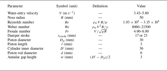

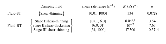

 V=3.43

 V=3.43ms−1
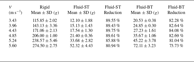
 ±

 V=3.43 ms−1

 CR
 Vt/R

 CR
 V=3.96
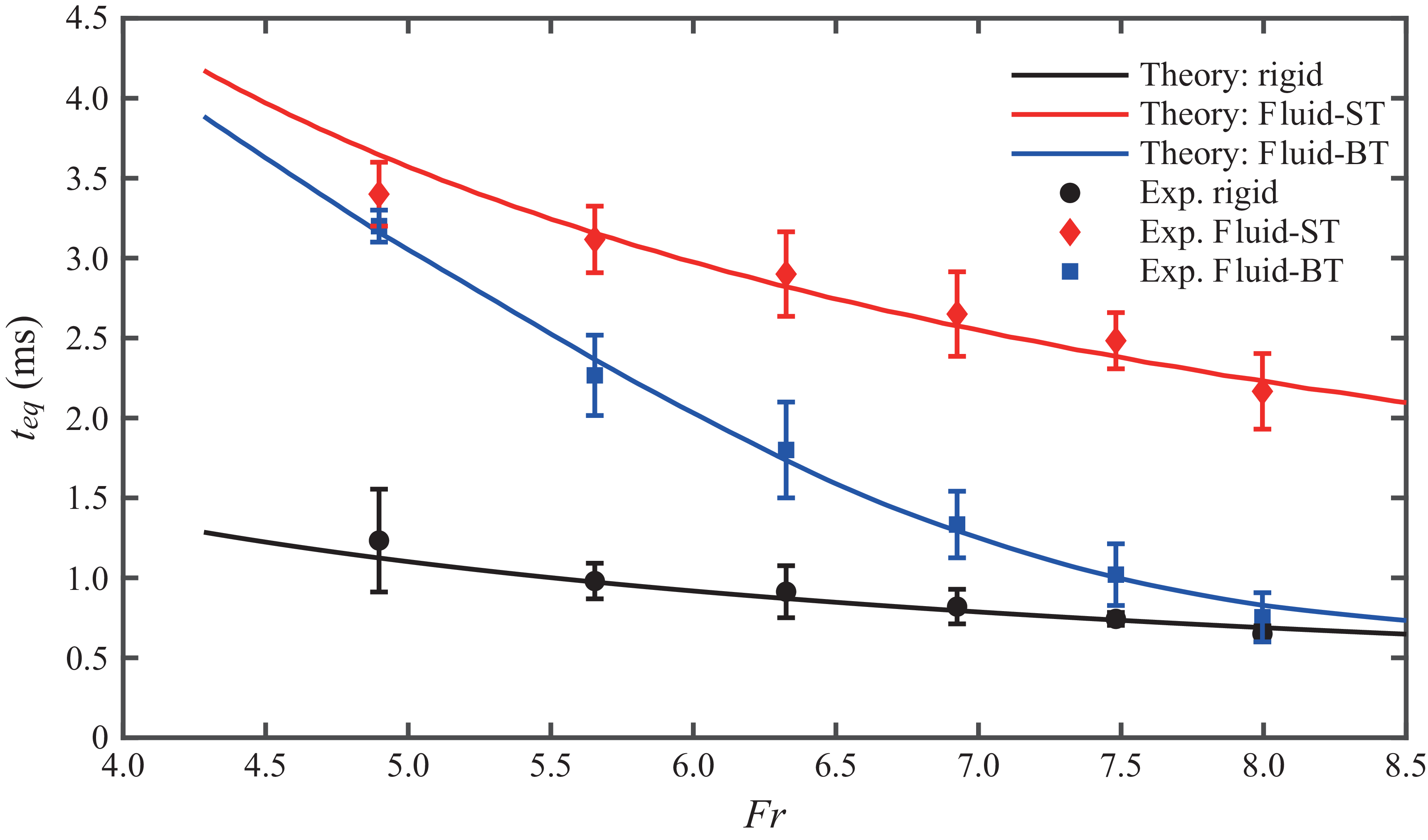
 teq
 Fr
 teq


 A^(f)=A(f)/Amax
 ±
 1760±50 Hz
 20±2 Hz
 20±2 Hz
 39±3 Hz

 K
 α


 h0
 h0

 V=3.43
 3.96
 4.43
 4.85
 5.24
 5.60 ms−1

 D0
 D0=40 mm



