2.1 Overview of the applicability of the CEL method

Sled helicopters cause significant deformation of snow when landing on snow-covered pavement. Traditional Lagrangian methods fail to converge due to mesh distortion under large deformations, limiting their applicability in such scenarios. The CEL method effectively addresses this large deformation challenge. During coupling, Lagrangian elements occupy space within the Eulerian mesh, calculating interactions with objects in Eulerian elements through contact algorithms. Since the material of a large-deformation object can flow within the Euler grid, the object material does not completely fill the Euler grid. The CEL method employs an Euler volume fraction to describe the proportion of object material within the grid. An Euler volume fraction of 1 indicates that the Euler grid is filled with material, while an Euler volume fraction of 0 indicates that the Euler grid is empty and not filled with material.

2.2 Simulation model of plate sinking

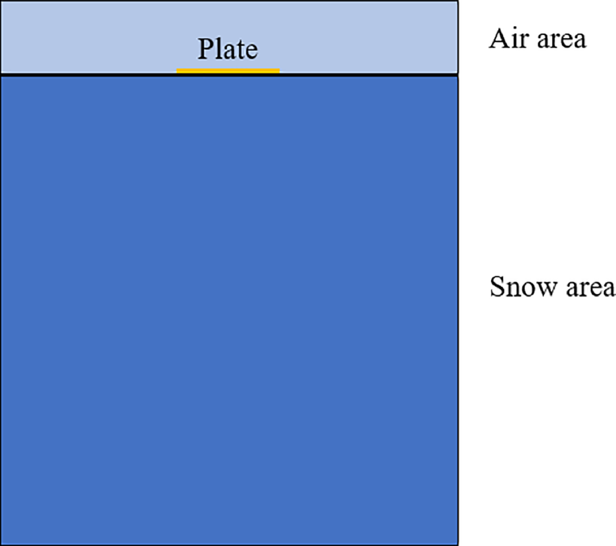
This section employs the CEL method to simulate and validate the load-bearing behaviour of a plate sinking into snow. The plate, with a diameter of 20 cm, is modeled as a Lagrangian body. The snow, measuring 60 cm in diameter and 39.2 cm in thickness, is modeled as an Eulerian body. Additionally, an air pocket is reserved above the snow region to facilitate the displacement of snow material into this air space during the plate’s descent. The initial state is set with the plate just contacting the snow surface. Uniform plate descent is achieved through displacement control, thereby constructing the load–displacement relationship curve. The model schematic is shown in Fig. 1.

Table 1.

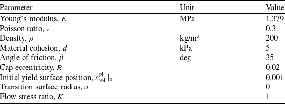
Modified CDP snow model parameters

Table 1 Long description

A table with 8 rows and 3 columns. The columns are labeled Parameter, Unit, and Value. The table lists various parameters of the modified CDP snow model along with their respective units and values. Row 1: Parameter, Young's modulus, E; Unit, MPa; Value, 1.379. Row 2: Parameter, Poisson ratio, v; Unit, none; Value, 0.3. Row 3: Parameter, Density, ρ; Unit, kg/m3; Value, 200. Row 4: Parameter, Material cohesion, d; Unit, kPa; Value, 5. Row 5: Parameter, Angle of friction, β; Unit, deg; Value, 35. Row 6: Parameter, Cap eccentricity, R; Unit, none; Value, 0.02. Row 7: Parameter, Initial yield surface position, ε_vol^pl|_0; Unit, none; Value, 0.001. Row 8: Parameter, Transition surface radius, a; Unit, none; Value, 0. Row 9: Parameter, Flow stress ratio, K; Unit, none; Value, 1.

Figure 1.

Simulation of plate sinking based on the CEL method.

In terms of snow characterisation, to align with natural polar snow environments, the CDP constitutive model parameters for low-density natural snow [Reference Haehnel and Shoop24] were adopted as the baseline model parameters. Subsequently, these parameters were iteratively optimised based on CEL simulation results to derive snow constitutive model material parameters suitable for the CEL simulation method, as shown in Table 1.

2.3 Comparison of simulation and experimental results

Figure 2 illustrates the morphological changes in snow accumulation after the plate sinks into snow. The colours in Fig. 2(a) represent the degree of snow accumulation within the grid cells. As shown in Fig. 2(b), the snow beneath the plate exhibits significant compaction characteristics under pressure, consistent with the actual deformation patterns of natural snow under loading. This method effectively simulates the interaction between the plate and snow accumulation, validating the rationality of the model geometry and load transfer settings.

Figure 2.

Status changes diagram of snow. (a) Snow deformation diagram. (b) Snow stress diagram.

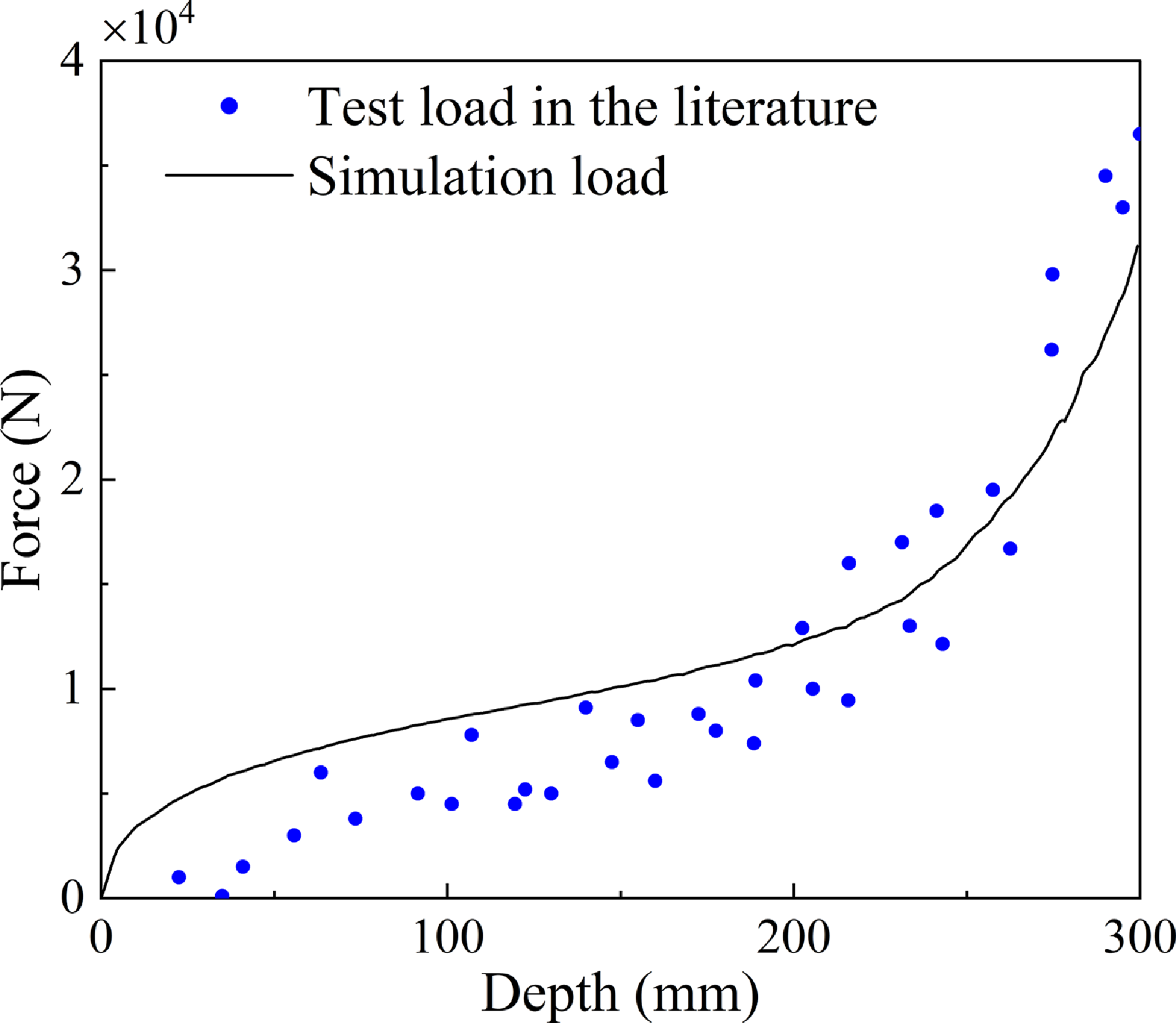
Figure 3 presents the comparison of displacement-load curves under plate sinking. Compared to experimental data from the literature [Reference Haehnel and Shoop24], the evolution trend of the simulation results aligns well with the test data. This result validates the effectiveness of the CEL method and CDP constitutive model in reflecting the mechanical properties of low-density snow under rapid loading conditions, laying a foundational model for subsequent analysis of sled helicopter landing characteristics.

Figure 3.

Comparison of simulation curves and experimental results.

3.1 Sled helicopter finite element model

In the field of finite element analysis, geometric model simplification is a critical step. Complex geometric models often require a large number of elements and nodes during discretisation, which significantly increases computational demands. By simplifying the geometric model, the number of elements can be effectively reduced, thereby lowering computational complexity and time costs, ultimately improving computational efficiency. Therefore, this paper employs a reasonable simplification for the sled helicopter. The fuselage structure modelling is omitted, and the fuselage weight is simulated by applying a mass point at the fuselage location. The sled landing gear is modelled as a solid, and the connections between components are simulated using kinematic joints.

3.1.1 Tire model

Aircraft tires feature a complex structure, primarily composed of tread, shoulder, carcass, sidewall, bead and belt layers [Reference Yang28]. Their material composition mainly consists of isotropic rubber materials and relatively complex cord-rubber composite materials. This paper disregards other tire materials and employs an isotropic, incompressible rubber material for finite element modelling. A solid model of the landing gear tire for a sled helicopter is constructed, with specific dimensional parameters shown in Table 2.

Table 2.

Tire geometric parameters

Table 2 Long description

A table comparing tire geometric parameters for aircraft landing gear. The table has two rows and three columns. The columns are labeled Diameter (cm), Width (cm), and Landing Gear Type. The first row compares the tail landing gear with a diameter of 46 centimeters and a width of 14 centimeters. The second row compares the main landing gear with a diameter of 68 centimeters and a width of 22 centimeters.

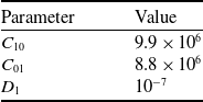
Aircraft tires undergo significant deformation when inflated and subjected to ground loads. The rubber material used in aviation tires is a typical hyperelastic material exhibiting highly nonlinear characteristics, primarily manifested in both material properties and geometric features. When characterising the mechanical properties of hyperelastic rubber materials, their stress-strain relationship is primarily described using strain energy. The Mooney–Rivlin hyperelastic constitutive model, widely applied in engineering for elastomer deformation, is employed to describe the tire material. Specific parameter values [Reference Cai and Xu29] are shown in Table 3.

Table 3.

Tire material property parameters

Table 3 Long description

A table showing tire material property parameters with two columns and three rows. The columns are labeled Parameter and Value. The rows are as follows: Row 1: Parameter, C 10; Value, 9.9 times 10 to the power of 6. Row 2: Parameter, C 01; Value, 8.8 times 10 to the power of 6. Row 3: Parameter, D 1; Value, 10 to the power of -7.

Additionally, the tires were discretised into a mesh composed entirely of hexahedral elements, with the element type designated as C3D8R. The main landing gear tires comprised 34,580 elements, while the single tail landing gear tire contained 27,840 elements. The mesh model is illustrated in Fig. 4.

3.1.2 Sled model

When landing on snow-covered pavement in polar regions and high latitudes, the sled plays a critical role for the sled helicopter. To enhance computational efficiency, the sleds were appropriately simplified by removing certain chamfers, small holes, bolt connections and other components, while retaining their primary structure. The configuration dimensions of the sleds are shown in Table 4. Since structural deformation of the sleds is negligible compared to snow morphology changes during interaction, the sleds are treated as a rigid body in the analysis. A discrete mesh was generated for the sleds using C3D8R hexahedral elements. The tail landing gear sled comprised 17,754 elements, while the main landing gear sled contained 48,963 elements. The sled mesh model is illustrated in Fig. 5.

Table 4.

Sled dimension parameters

Table 4 Long description

A table comparing dimensions of landing gear sleds. The table has two rows and four columns. The columns are labeled Length (mm), Width (mm), and Camber angle (°). The row labels are Main landing gear sled and Tail landing gear sled. Row 1: Main landing gear sled, Length (mm) 2,200, Width (mm) 700, Camber angle (°) 12. Row 2: Tail landing gear sled, Length (mm) 1,600, Width (mm) 880, Camber angle (°) 14.

Figure 4.

Tire mesh model diagram. (a) Tail landing gear tire mesh model. (b) Main landing gear tire mesh model.

Figure 5.

Sled mesh model diagram. (a) Main landing gear sled. (b) Tail landing gear sled.

3.1.3 Equivalent buffer model

The landing gear buffer primarily serves to absorb impact energy during aircraft landing and support the fuselage load during sliding, thereby rapidly damping fuselage vibrations. The axial force within the buffer ( ${F_V}$ ) is mainly composed of gas spring force ( ${F_s}$ ), hydraulic damping force ( ${F_d}$ ), buffer friction force ( ${F_f}$ ) and structural restraint force exerted on the buffer when uncompressed [Reference Wu, Nie, Zhang and Shi30]:

(1) \begin{align}{F_V} = \left\{ {\begin{array}{c@{\quad}c}{{K_{st}}}\\{{F_s} + {F_d} + {F_f}}\\{{K_{sc}}({L_M} - {L_{\max }})}\end{array}} \right.{\rm{ }}\begin{array}{*{20}{c}}{{L_M} \lt 0}\\{0 \lt {L_M} \lt {L_{\max }}}\\{{L_M} \geqslant {L_{\max }}}\end{array}\end{align}

In the formula: ${K_{st}}$ and ${K_{sc}}$ represent the tensile stiffness and compressive stiffness of the strut related to structural restraint forces; ${L_{\max }}$ denotes the maximum compression stroke of the buffer; ${L_M}$ indicates the buffer compression amount.

The expression for the force of the gas spring is as follows:

(2) \begin{align}{F_s} = {A_a}\left[ {{P_0}{{\left( {\frac{{{V_0}}}{{{V_0} - {A_a}{L_M}}}} \right)}^{{n_0}}} - {P_{atm}}} \right]\end{align}

In the formula: ${A_a}$ represents the effective gas-filled area of the buffer; ${P_0}$ denotes the initial gas pressure of the buffer; ${V_0}$ indicates the initial gas volume of the buffer; ${n_0}$ signifies the gas polytropic index; ${P_{atm}}$ represents the local atmospheric pressure.

The expression for the hydraulic damping force is as follows:

(3) \begin{align}{F_d} = \left\{ {\begin{array}{*{20}{c}}{\left( {\dfrac{{{\rho _0}A_h^3}}{{2C_d^2A_d^2}}} \right)\mathop {L_M^2}\limits^ \bullet\quad {\rm{ }}{{\mathop L\limits^ \bullet }_M} \geqslant 0}\\[12pt]{ - \left( {\dfrac{{{\rho _0}A_h^3}}{{2C_d^2A_{dl}^2}}} \right)\mathop {L_M^2}\limits^ \bullet \quad{\rm{ }}{{\mathop L\limits^ \bullet }_M} \lt 0}\end{array}} \right.\end{align}

In the formula: ${\rho _0}$ represents the density of the buffer’s filling fluid; ${A_h}$ denotes the effective oil pressure area of the buffer’s oil chamber; ${C_d}$ indicates the flow restriction coefficient of the oil chamber’s orifice; ${A_d}$ and ${A_{dl}}$ represent the oil hole areas for the positive and return strokes, respectively; ${\mathop L\limits^ \bullet _M}$ signifies the buffer’s compression velocity.

The buffer friction force consists of two components [Reference Liang31]: sealing friction ${f_1}$ generated by the internal pressure within the buffer and structural friction ${f_2}$ caused by the bending of the buffer strut, as shown in the following equation:

(4) \begin{align}{F_f} = {f_1} + {f_2}\end{align}

The expression for ${f_1}$ is

(5) \begin{align}{f_1} = {\mu _m}{F_s}\frac{{\mathop {{l_M}}\limits^ \bullet }}{{\mathop {|{l_M}|}\limits^ \bullet }}\end{align}

The expression for ${f_2}$ is

(6) \begin{align}{f_2} = {\mu _b}(|{N_u}| + |{N_1}|)\frac{{\mathop {{l_M}}\limits^ \bullet }}{{|\mathop {{l_M}}\limits^ \bullet |}}\end{align}

In the formula: ${\mu _m}$ is the equivalent sealing friction coefficient, ${\mu _b}$ is the coulomb friction coefficient, ${N_u}$ and ${N_1}$ are the positive pressures at the upper and lower support points of the pillar.

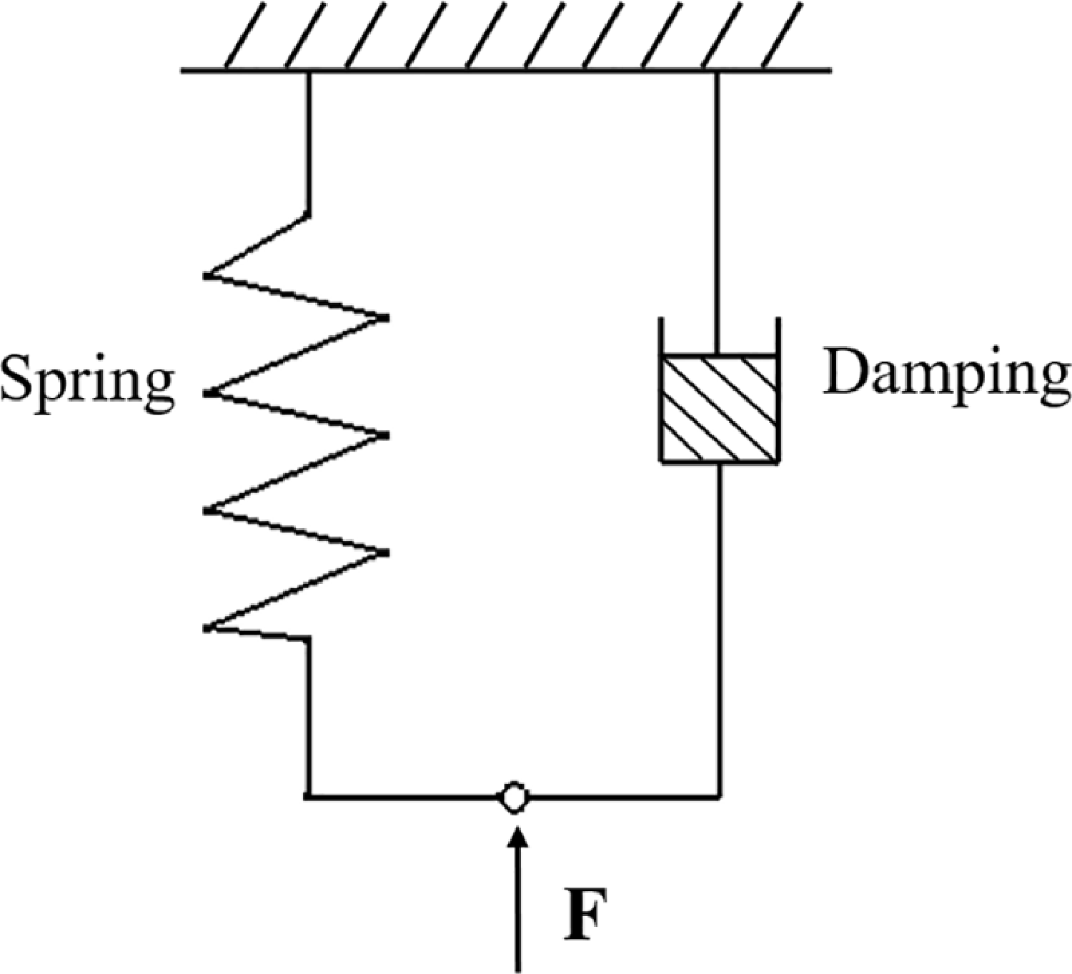
Since the friction force of the buffer is significantly smaller than the gas spring force and the hydraulic damping force, it can be considered negligible. Therefore, this section models only the gas spring force and hydraulic damping force for the landing gear buffer in the finite element analysis. The structural restraint force applied to the buffer in its uncompressed state is applied at the initial compression moment of the spring force. The simplified physical model of the buffer is shown in Fig. 6.

Figure 6.

Simplified diagram of the buffer.

3.2 Finite element model of snow-covered pavement

In this analysis, the snow-covered pavement model is defined as an Eulerian body and divided into an Eulerian mesh with EC3D8R element type. Since the air domain has a negligible impact on simulation results, the air domain mesh size is appropriately enlarged to enhance computational efficiency and reduce computational costs, while the snow domain mesh is densified. To ensure simulation results remain unaffected by mesh density variations, the snow domain mesh size was tested at three levels: 25, 20 and 15 mm. Balancing computational cost and accuracy, the snow domain element size was finalized at 15 mm, while the air domain element size was set to 40 mm. The snow depth was set to 392 mm. In the vertical landing simulation scenario, the snow model comprises a total of 636,861 grid cells. In the sled helicopter sliding landing simulation, the size of the snow-covered area depends on the helicopter’s heading velocity.

Due to the extensive snow-covered pavement in actual conditions, non-reflecting boundaries were applied to the sides of the snow-covered area to eliminate the boundary effect’s impact on simulation results. The bottom of the snow model closely adheres to the concrete pavement, which is modeled as a rigid body. The snow model under the landing simulation conditions of the sled helicopter is shown in Fig. 7.

Figure 7.

Snow mesh model diagram.

3.3 Multi-physics-coupled finite element model of helicopters and snow-covered pavement

The helicopter’s main landing gear employs a single-wheel swing arm configuration, while the tail landing gear utilises a dual-wheel strut design. Prior to analysing snow landings, a coordinate system must be defined to establish reference directions for subsequent load application and data output. Define the origin ${O_E}$ of the snow surface coordinate system ${O_E}{X_E}{Y_E}{Z_E}$ as the projection point of the helicopter’s centre of gravity onto the snow surface. The ${O_E}{X_E}$ axis is parallel to the ground and points forward as positive, the ${O_E}{Z_E}$ axis points vertically upward and the ${O_E}{Y_E}$ axis follows the right-hand rule. The origin ${O_b}$ of the fuselage coordinate system ${O_b}{X_b}{Y_b}{Z_b}$ is located at the helicopter’s centre of gravity. The ${O_b}{X_b}$ axis points forward toward the nose as positive, the ${O_b}{Z_b}$ axis is perpendicular to the ${O_b}{X_b}$ axis and points downward towards the fuselage as positive and the ${O_b}{Y_b}$ axis follows the right-hand rule. In the finite element software, the sled helicopter and snow model are assembled in their initial positions, as shown in Fig. 8.

Figure 8.

Helicopter and snow assembly diagram.

4.1 Analysis of symmetrical vertical landing characteristics

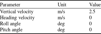
Due to the sled installed on the landing gear, the sled helicopter has a larger contact area with the snow during the landing phase. This results in a significant difference in the cushioning effect of snow between wheeled helicopters and sled helicopters. This subsection compares the symmetrical vertical landing characteristics of wheeled and sled helicopters on snow-covered pavement. Initial landing parameters are shown in Table 5.

Table 5.

Symmetrical vertical landing parameters

Table 5 Long description

A table comparing vertical landing parameters for helicopters. The table has three columns and five rows. Column headers are Parameter, Unit, and Value. Row 1: Parameter, Vertical velocity, Unit, m/s, Value, 2.5. Row 2: Parameter, Heading velocity, Unit, m/s, Value, 0. Row 3: Parameter, Roll angle, Unit, deg, Value, 0. Row 4: Parameter, Pitch angle, Unit, deg, Value, 0.

Figure 9.

Diagram of the landing state of the wheeled helicopter.

Figure 10.

Diagram of the landing state of the sled helicopter.

Figures 9 and 10 show the landing states of the wheeled helicopter and the sled helicopter, respectively. The diagrams clearly show the landing state of the helicopters on snow-covered pavement. Compared to the wheeled helicopters, the sled helicopter exhibits shallower displacement when sinking into the snow.

Figure 11 depicts the sled–tire load distribution curves during the landing phase of the sled helicopter. It can be seen that the maximum peak load on the main landing gear sled is 28,985 N, which is 5.92 times the maximum peak load on the tire. The maximum peak load ratio between the sled and tire on the tail landing gear is 4.66:1. This indicates that the sled bears the primary landing load during the landing process.

Figure 11.

Sled – tire load distribution curves. (a) Main landing gear. (b) Tail landing gear.

The state change curve of the helicopter during symmetrical vertical landing is shown in Fig. 12. Figure 12(a) and (b) reveals that the wheeled helicopter sinks deeper into the snow than the sled helicopter. During a smooth landing, the main landing gear of the wheeled helicopter sinks 0.373 m into the snow, while the sled helicopter sinks 0.288 m – a reduction of 22.79% compared to the wheeled helicopter. This demonstrates that the wheeled helicopter exhibits some rebound during landing, whereas the sled helicopter does not. This occurs because when the landing gear contacts the snow surface, the soft nature of the snow allows the gear to continue sinking, accelerating its velocity. In contrast, the wheeled landing gear has a smaller contact area with the snow, preventing the snow from providing effective support. The tires compact the snow, transforming it into a near-hard surface. In contrast, the sled landing gear, equipped with the sled, increases the contact area with the snow. The sled bears the primary load, and through the interaction between the sled and the snow, the landing gear stabilises rapidly.

Figure 12.

Helicopter state variation curve during symmetrical vertical landing. (a) Main landing gear buried in snow depth. (b) Vertical displacement of centre of mass. (c) Vertical velocity of the centre of mass. (d) Vertical overload of the centre of mass.

Figure 12(c) shows the variation curve of the centre of gravity sinking velocity. It can be observed that before 0.2 s, the sinking velocity of the helicopter’s centre of gravity continues to increase, reaching 2.74 m/s for the wheeled helicopter and 2.64 m/s for the sled helicopter. Figure 12(d) shows the vertical overload curve of the centre of gravity. It can be seen that the maximum vertical overload of the wheeled helicopter’s centre of gravity is 1.48 g, while that of the sled helicopter is 1.11 g, a 25% reduction compared to the wheeled helicopter. This is because the sled landing gear has a larger contact area with the snow, and the snow provides more favourable cushioning for the sled helicopter compared to the wheeled helicopter.

Figure 13 depicts the buffer state change curves for two helicopter types during the symmetrical vertical landing phase. As shown in Fig. 13(a) and (b), after the snow-covered pavement provides an effective support force, the maximum compression displacement of the tail landing gear buffer for both helicopter types is similar, both around 0.32 m. The maximum compression velocity of the tail landing gear buffer for the wheeled helicopter is 2.07 m/s, while that for the sled helicopter is 1.62 m/s, representing a 21.74% reduction compared to the wheeled helicopter.

Figure 13.

State variation curve of helicopter buffer during symmetrical vertical landing. (a) Tail landing gear buffer compression displacement. (b) Tail landing gear buffer compression rate. (c) Main landing gear buffer compression displacement. (d) Main landing gear buffer compression rate. (e) Power diagram of the tail landing gear. (f) Power diagram of the main landing gear.

Figure 13(e) and (f) depicts the buffer energy diagrams for the tail landing gear and main landing gear, respectively. The buffer efficiencies for the wheeled tail landing gear and main landing gear are 73.10% and 78.24%, respectively. Under identical damper parameters, the buffer efficiencies for the sled tail landing gear and main landing gear were 82.58% and 82.92%, respectively. This discrepancy arises because the initial compression rate of the wheeled helicopter buffer is significantly higher. Consequently, the peak load generated by the hydraulic fluid damping force substantially exceeds the load corresponding to the gas spring force, adversely affecting buffer efficiency.

4.2 Analysis of asymmetric vertical landing characteristics

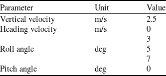
This section analyses the asymmetric vertical landing characteristics of the sled helicopter on snow-covered pavement with an initial roll angle. Initial landing parameters are shown in Table 6. When landing with a positive roll angle, the helicopter’s right wheel touches down first.

Table 6.

Asymmetric vertical landing parameters

Table 6 Long description

A table showing vertical landing parameters with three columns and five rows. The columns are labeled Parameter, Unit, and Value. The parameters listed are Vertical velocity, Heading velocity, Roll angle, and Pitch angle. The units for velocity are meters per second, and for angles, degrees. The values are Vertical velocity 2.5 meters per second, Heading velocity 0 meters per second, Roll angle 5 degrees, Pitch angle 7 degrees, and Pitch angle 0 degrees.

Figure 14 depicts the state variation curves of a helicopter during asymmetric vertical landing. As shown in Fig. 14(a), the vertical overloads at the centre of gravity exhibit minimal variation across landing conditions with roll angles of 3°, 5° and 7°, measuring 1.1, 1.13 and 1.17 g, respectively. Figure 14(b), (c) and (d) presents the snow penetration depth curves for the helicopter landing gear. It should be noted that when the right landing gear touches down, the tail landing gear and left main landing gear have not yet contacted the snow surface, resulting in an initial height greater than zero. It can be observed that as the roll angle increases, the right landing gear and tail landing gear sink deeper into the snow, while the left landing gear exhibits the opposite trend. Specifically, the right landing gear sinks to a depth of 0.302 m during landing at a 3° roll angle, while the sinking depths at 5° and 7° roll angles are 2.65% and 5.96% greater than that at 3°, respectively. Figure 14(e) shows the roll angle variation curve of the helicopter. After landing on snow, the roll angle first decreases rapidly, then gradually increases and stabilises. Under the 3°, 5° and 7° roll angle landing conditions, the roll angle ultimately stabilises at 1.5°, 2.34° and 2.96°, respectively. As shown in the roll angle velocity curve in Fig. 14(f), the maximum roll angle velocity under the 3° roll angle landing condition is 7.35°/s. In contrast, the roll angle velocities under the 5° and 7° roll angle landing conditions are 60.41% and 115.92% higher than that under the 3° roll angle condition, respectively.

Figure 14.

Helicopter state variation curve during asymmetric vertical landing. (a) Vertical centre of gravity overload. (b) Tail landing gear retraction depth. (c) Right landing gear retraction depth. (d) Left landing gear retraction depth. (e) Roll angle. (f) Roll angular velocity.

The variation curves of main landing gear support force and lateral force during asymmetric vertical landing are shown in Fig. 15. As seen in Fig. 15(a) and (c), the greater the roll angle of the sled helicopter, the larger the support force on the right landing gear. At a 0° roll angle, the peak support load reaches 33,705 N, occurring when the hydraulic damping force is maximum. At 3°, 5° and 7° roll angles, peak support loads are 37,222 N, 41,418 N and 46,873 N, respectively – representing increases of 10.43%, 22.88% and 39.07% compared to the 0° roll angle condition. These peaks occur at the moment of maximum gas spring force. This occurs because a larger initial landing roll angle subjects the right landing gear to greater fuselage weight, intensifying the stress on the landing gear. Conversely, as the initial landing roll angle of the sled helicopter increases, the left landing gear experiences forces later, resulting in reduced support capacity. Figure 15(b) and (d) shows the lateral force variation curves for the main landing gear. As the initial landing roll angle of the sled helicopter increases, the lateral forces on the main landing gear also increase.

Figure 15.

Variation curve of ground forces acting on the helicopter during asymmetric vertical landing. (a) Right landing gear support force. (b) Right landing gear lateral force. (c) Left landing gear support force. (d) Left landing gear lateral force.

Figure 16 shows the state change curve of the main landing gear buffer under asymmetric vertical landing conditions. From Fig. 16(a) and (b) of the buffer compression displacement curve, the maximum compression values for the right landing gear buffer under 3°, 5° and 7° roll angle landing conditions are 0.335, 0.352 and 0.365 m, respectively, which are 20.07%, 35.91% and 52.72% higher than those of the left landing gear. Since the helicopter’s right landing gear contacts the ground first and remains in a tilted posture after sinking into snow, it bears a greater portion of the fuselage weight compared to the left landing gear.

Figure 16.

Helicopter buffer status variational curve during asymmetric vertical landing. (a) Right landing gear buffer compression displacement. (b) Left landing gear buffer compression displacement. (c) Right landing gear buffer compression rate. (d) Left landing gear buffer compression rate. (e) Power diagram of the right landing gear. (f) Power diagram of the left landing gear.

Figure 16(c) and (d) shows the compression velocity curves of the main landing gear buffer. It can be observed that for different roll angle landing conditions, the compression velocity of the right landing gear buffer remains relatively stable; however, as the roll angle increases, the peak compression velocity of the left landing gear buffer decreases. Figure 16(e) and (f) show the landing gear buffer energy diagrams. Under landing conditions with roll angles of 3°, 5° and 7°, the right landing gear buffer efficiencies were 75.22%, 69.69% and 64.27%, respectively. Meanwhile, the left landing gear buffer efficiencies were 84.97%, 84.01% and 82.63%, respectively. This occurs because as the initial landing roll angle of the sled helicopter increases, the weight allocated to the right landing gear significantly rises. Consequently, the peak load generated by the gas spring force of the landing gear buffer substantially exceeds the load corresponding to the hydraulic damping force, adversely affecting buffer efficiency.

4.3 Safety analysis of sled helicopter sliding landings

In order to ensure the safety and reliability of the aircraft, it is generally necessary to take measures to avoid accidents or disasters [Reference Xiang, Xie, Ye, Yan, Han, Niu, Li and Huang32]. Compared to conventional hard surfaces, snow-covered pavement presents unique characteristics that result in greater heading resistance for sled landing gear during sliding. This increased resistance generates a larger nose-down moment on the helicopter, potentially leading to a rollover. Therefore, to analyse the safety of the sled helicopter during snow pavement sliding landing, this section conducts a simulation analysis on landing and sliding safety boundary, considering the influence of initial landing velocity.

4.3.2 Analysis of sled helicopter sliding landing

Figure 17 depicts the pitch state variation curve of the sled helicopter during landing without pitch moment. As shown in Fig. 17(a), when landing at a heading velocity of 3 m/s, the attitude of the sled helicopter first pitches down, then pitches up and eventually stabilises, with a minimum pitch angle of −4.92°, indicating a safe landing condition. When the heading velocity increases to 3.8 m/s, the minimum pitch angle reaches −8°, precisely at the critical safety threshold. However, during landing at a heading velocity of 6 m/s, the minimum pitch angle drops below −30°, causing the helicopter to experience forward overturning.

Figure 17.

Pitch state variational curve of the sled helicopter without pitching moment. (a) Pitch angle variation curve. (b) Pitch angle velocity variation curve.

Figure 17(b) shows the pitch angular velocity curve. It can be observed that during the initial landing phase, the pitch angular velocity decreases rapidly. Subsequently, around 0.4 s, a rapid upward trend emerges. This is due to the main landing gear compressing into the snow surface and bearing most of the fuselage weight, causing a rebound phenomenon. At heading velocities of 3 and 3.8 m/s, the pitch angular velocity reaches zero, marking the moment of minimum roll angle.

Figure 18 depicts the landing velocity-moment safety boundary for a sled helicopter during a sliding landing. It shows that when the heading velocity is below 3.8 m/s, the helicopter can land safely relying on its inherent stability. However, when the heading velocity exceeds 3.8 m/s, the helicopter faces a risk of overturning during landing. In this scenario, the rotor must provide pitch moment to ensure a safe landing.

Figure 18.

Sled helicopter landing velocity-moment safety boundary.

Figure 19(a) shows the two-dimensional mapping curve of the velocity-moment safety boundary for a sled helicopter. It can be observed that during the helicopter sliding landing phase, the heading velocity significantly influences the magnitude of the minimum safe pitch moment, exhibiting a high degree of linearity. This phenomenon results from the interaction between the sled landing gear and accumulated snow. In contrast, the initial vertical velocity exerts a lesser influence. This is because the minimum pitch angle of the helicopter body occurs around 2 s, at which point the depth of main landing gear penetration into snow is similar across different initial vertical velocity conditions. Consequently, snow also imposes similar heading resistance on the sled helicopter, as illustrated by the vertical displacement variation curve of the main landing gear axle in Fig. 19(b).

Figure 19.

Two-dimensional mapping safety boundary curve. (a) Two-dimensional mapping curve of velocity and moment. (b) Vertical displacement curve of the main landing gear wheel axle at Vx = 6 m/s.