1 Introduction
Wake meandering, a large-scale lateral motion of the turbine wake, has been extensively studied experimentally (Medici & Alfredsson Reference Medici and Alfredsson2008; Iungo et al. Reference Iungo, Viola, Camarri, Porté-Agel and Gallaire2013; Okulov et al. Reference Okulov, Naumov, Mikkelsen, Kabardin and Sørensen2014; Howard et al. Reference Howard, Singh, Sotiropoulos and Guala2015) and computationally (Kang, Yang & Sotiropoulos Reference Kang, Yang and Sotiropoulos2014; Foti et al. Reference Foti, Yang, Guala and Sotiropoulos2016) for a single wind turbine. Studies have shown that the turbine nacelle induces a large-scale slowly precessing spiral vortex in the near field that can have a significant effect on wake meandering several rotor diameters downwind. Further studies (Schümann, Pierella & Stran Reference Schümann, Pierella and Sætran2013; Debnath et al. Reference Debnath, Santoni, Leonardi and Iungo2017; Santoni et al. Reference Santoni, Carrasquillo, Arenas-Navarro and Leonardi2017) have shown that the turbine nacelle and tower affect the wake symmetry. The effect of such phenomena at the turbine scale on the emergent turbine wake dynamics in a wind farm, however, have never been investigated before and remain poorly understood. The clustering of wind turbines in wind farms, typically within a few turbine rotor diameters apart, gives rise to the coalescence and interaction of turbine wakes, which can have significant effects on wake meandering, the power extraction and the dynamic loads on downwind turbines. Studies of turbine arrays and wind farms have been carried out extensively in the literature (Cal et al. Reference Cal, Lebrón, Castillo, Kang and Meneveau2010; Lu & Porté-Agel Reference Lu and Porté-Agel2011; Porté-Agel et al. Reference Porté-Agel, Wu, Lu and Conzemius2011; Yang, Kang & Sotiropoulos Reference Yang, Kang and Sotiropoulos2012; Archer, Mirzaeisefat & Lee Reference Archer, Mirzaeisefat and Lee2013; Stevens, Graham & Meneveau Reference Stevens, Graham and Meneveau2014; VerHulst & Meneveau Reference VerHulst and Meneveau2014; Nilsson et al. Reference Nilsson, Ivanell, Hansen, Mikkelsen, Sørensen, Breton and Henningson2015; Wu & Porté-Agel Reference Wu and Porté-Agel2015; Stevens, Martínez-Tossas & Meneveau Reference Stevens, Martínez-Tossas and Meneveau2018; Yang, Pakula & Sotiropoulos Reference Yang, Pakula and Sotiropoulos2018). These studies, however, employed wind turbine parameterisations that do not properly incorporate the effects of the nacelle and because of that, it is still not clear how turbine nacelle-induced coherent structures impact phenomena at the wind farm scale. Recently, Yang & Sotiropoulos (Reference Yang and Sotiropoulos2018) proposed a new actuator surface model that can accurately and efficiently incorporate the effects of the wind turbine nacelle on turbine wake development and dynamics. The model has been shown to be able to account for the effects of the nacelle both in the near-field and far-field (wake meandering) regions of a single turbine wake. In this work we seek to employ the model of Yang & Sotiropoulos (Reference Yang and Sotiropoulos2018) to evaluate effects of turbine-induced coherent structures at the wind farm scale. For that, we carry out two large-eddy simulations (LES) of a utility-scale offshore wind farm, the Horns Rev wind farm, using parameterisation with and without the turbine nacelles respectively, while keeping all other parameters in the simulations the same, and conduct a systematic analysis of the resulting flow fields to assess and quantify the effect of turbine nacelles on wind farm wake development and dynamics.
Recent investigations of wind farms attempt to explore causes of power losses or to gain insights into mean flow field statistics. Several studies (Meyers & Meneveau Reference Meyers and Meneveau2010; Stevens, Gayme & Meneveau Reference Stevens, Gayme and Meneveau2013) have focused on turbine positioning to minimise the power losses, which can be quite significant for tightly packed wind turbines (Barthelmie et al. Reference Barthelmie, Frandsen, Rathmann, Hansen, Politis, Prospathopoulos, Cabezon, Rados, van der Pijl and Schepers2008). Others have tackled more fundamental physics including the important driving factor for power extraction in the centre of wind farms, namely, the downward entrainment of energy through the vertical momentum flux (Frandsen Reference Frandsen1992; Cal et al. Reference Cal, Lebrón, Castillo, Kang and Meneveau2010; VerHulst & Meneveau Reference VerHulst and Meneveau2014). Offshore wind turbines and farms have also been studied computationally to ascertain the relationship among waves, atmospheric boundary layer and wind turbine aerodynamics (Yang, Meneveau & Shen Reference Yang, Meneveau and Shen2014a ,Reference Yang, Meneveau and Shen b ; Calderer et al. Reference Calderer, Guo, Shen and Sotiropoulos2018). However, the dynamics of wind turbine wakes in utility-scale wind farms, and especially the effects of turbine nacelle geometry and the coherent structures it induces on wind-farm-scale turbine wake dynamics, has yet to be investigated and understood.
The effects of the turbine nacelle on the genesis of a slowly precessing helical hub vortex, which expands in the radial direction and interacts with the rotor tip shear layer augmenting wake meandering intensity several rotor diameters downwind, have recently been well documented for a single wind turbine (Kang et al. Reference Kang, Yang and Sotiropoulos2014; Foti et al. Reference Foti, Yang, Guala and Sotiropoulos2016, Reference Foti, Yang, Campagnolo, Maniaci and Sotiropoulos2018a ). However, the effects of the nacelle and hub vortex on turbine wakes in wind farms, wake–wake interactions and wake–atmospheric flow interactions are still unknown, especially consequences of the effects of the nacelle on wake meandering within a wind farm. In this study, we endeavour to elucidate details about the interactions of the hub vortex, wake meandering and neighbouring turbine wakes. Furthermore, recent work (Foti, Yang & Sotiropoulos Reference Foti, Yang and Sotiropoulos2018b ) has shown that there is a similarity of scales of wake meandering among turbines of different sizes and designs. However, it is unclear if the similarity remains in wind farms with turbine–turbine wake interactions. In this work, we also seek to understand similarity of scales of wake meandering with and without a nacelle model in the well-studied offshore Horns Rev wind farm.
Therefore, the objective of this work is to assess the effects of wind turbine nacelles on the power output and the statistics of turbine wakes and wake meandering in a utility-scale wind farm using LES with a new class of actuator surface models for turbine blades and nacelles proposed by Yang & Sotiropoulos (Reference Yang and Sotiropoulos2018). Two cases, one with the turbine nacelles and the other without the turbine nacelles, are carried out. The wake meandering for the cases with and without a model for the nacelles is investigated using the wake meandering reconstruction technique of Foti et al. (Reference Foti, Yang, Guala and Sotiropoulos2016). This paper is set up first by reviewing the numerical methods in § 2 and the simulation parameters for the Horns Rev wind farm in § 3. The results are discussed in § 4, and the final conclusions are in § 5.
2 Numerical methods
We employ the LES module of the virtual flow simulator VFS-Wind code (Yang et al.
Reference Yang, Sotiropoulos, Conzemius, Wachtler and Strong2015) for the present cases. In VFS-Wind, we solve numerically the three-dimensional, incompressible, spatially filtered for LES continuity and momentum equations in generalised curvilinear coordinates (Ge & Sotiropoulos Reference Ge and Sotiropoulos2007) formulated as follows (
 $i,j=1,2,3$
and repeated indices imply summation):
 $$\begin{eqnarray}\displaystyle & \displaystyle J\frac{\unicode[STIX]{x2202}U^{i}}{\unicode[STIX]{x2202}\unicode[STIX]{x1D709}^{i}}=0, & \displaystyle\end{eqnarray}$$
 $$\begin{eqnarray}\displaystyle & \displaystyle \frac{1}{J}\frac{\unicode[STIX]{x2202}U^{i}}{\unicode[STIX]{x2202}t}=\frac{\unicode[STIX]{x1D709}_{l}^{i}}{J}\left(-\frac{\unicode[STIX]{x2202}}{\unicode[STIX]{x2202}\unicode[STIX]{x1D709}^{j}}(U^{j}u_{l})+\frac{\unicode[STIX]{x1D707}}{\unicode[STIX]{x1D70C}}\frac{\unicode[STIX]{x2202}}{\unicode[STIX]{x2202}\unicode[STIX]{x1D709}^{j}}\left(\frac{g^{jk}}{J}\frac{\unicode[STIX]{x2202}u_{l}}{\unicode[STIX]{x2202}\unicode[STIX]{x1D709}^{k}}\right)-\frac{1}{\unicode[STIX]{x1D70C}}\frac{\unicode[STIX]{x2202}}{\unicode[STIX]{x2202}\unicode[STIX]{x1D709}^{j}}\left(\frac{\unicode[STIX]{x1D709}_{l}^{j}p}{J}\right)-\frac{1}{\unicode[STIX]{x1D70C}}\frac{\unicode[STIX]{x2202}\unicode[STIX]{x1D70F}_{lj}}{\unicode[STIX]{x2202}\unicode[STIX]{x1D709}^{j}}\right)\!,\qquad & \displaystyle\end{eqnarray}$$
where
 $\unicode[STIX]{x1D709}^{i}$
are the curvilinear coordinates,
 $\unicode[STIX]{x1D709}_{l}^{i}=\unicode[STIX]{x2202}\unicode[STIX]{x1D709}^{i}/\unicode[STIX]{x2202}x_{l}$
are the transformation metrics,
 $J$
is the Jacobian of the geometric transformation,
 $u_{i}$
is the
 $i$
th component of the velocity vector in Cartesian coordinates,
 $U^{i}=(\unicode[STIX]{x1D709}_{m}^{i}/J)u_{m}$
is the contravariant volume flux,
 $g^{jk}=\unicode[STIX]{x1D709}_{l}^{j}\unicode[STIX]{x1D709}_{l}^{k}$
are the components of the contravariant metric tensor,
 $\unicode[STIX]{x1D70C}$
is the density,
 $\unicode[STIX]{x1D707}$
is the dynamic viscosity,
 $p$
is the pressure and
 $\unicode[STIX]{x1D70F}_{ij}$
represents the anisotropic part of the subgrid-scale stress tensor. The closure for
 $\unicode[STIX]{x1D70F}_{ij}$
is provided by a dynamic Smagorinsky model (Smagorinsky Reference Smagorinsky1963) developed by Germano et al. (Reference Germano, Piomelli, Moin and Cabot1991):
 $$\begin{eqnarray}\unicode[STIX]{x1D70F}_{ij}-{\textstyle \frac{1}{3}}\unicode[STIX]{x1D70F}_{kk}\unicode[STIX]{x1D6FF}_{ij}=-2\unicode[STIX]{x1D707}_{t}\widetilde{\unicode[STIX]{x1D61A}}_{ij},\end{eqnarray}$$
where the
 $\widetilde{(\cdot )}$
denotes the grid filtering operation, and
 $\widetilde{\unicode[STIX]{x1D61A}}_{ij}$
is the filtered strain-rate tensor. The eddy viscosity
 $\unicode[STIX]{x1D707}_{t}$
is given by
 $$\begin{eqnarray}\unicode[STIX]{x1D707}_{t}=\unicode[STIX]{x1D70C}C_{s}\unicode[STIX]{x1D6E5}^{2}|\tilde{\unicode[STIX]{x1D64E}}|,\end{eqnarray}$$
where
 $C_{s}$
is the dynamically calculated Smagorinsky coefficient (Germano et al.
Reference Germano, Piomelli, Moin and Cabot1991; Lilly Reference Lilly1992),
 $\unicode[STIX]{x1D6E5}$
is the filter size taken as the cubic root of the cell volume and
 $|\tilde{\unicode[STIX]{x1D64E}}|=(2\widetilde{\unicode[STIX]{x1D61A}}_{ij}\,\widetilde{\unicode[STIX]{x1D61A}}_{ij})^{1/2}$
. The governing equations are discretised using the three-point central, second-order accurate finite difference scheme and integrated in time using a second-order accurate projection method. The details of the numerical method used to solve the above equations and the numerical implementation of the dynamic Smagorinsky model can be found in Ge & Sotiropoulos (Reference Ge and Sotiropoulos2007) and Kang et al. (Reference Kang, Lightbody, Hill and Sotiropoulos2011).
The turbine blades and nacelles are represented with actuator surfaces using the recently developed model of Yang & Sotiropoulos (Reference Yang and Sotiropoulos2018). The blade geometry is represented by a surface formed by the chord lines with distributed forces along the chord. The forces are calculated in the same way as in the actuator line model using the blade element approach with tabulated blade twist angle and chord length at different radial locations, and lift and drag coefficients for different angles of attack. In the actuator surface model for nacelle, the nacelle geometry is represented by the actual surface of the nacelle with distributed forces. The force on the actuator surface is decomposed into two parts: the normal component and the tangential component. The normal component of the force is computed in a way to satisfy the no-penetration condition using the direct forcing immersed boundary approach (Uhlmann Reference Uhlmann2005). The tangential component of the force is computed using the incoming downwind velocity with a friction coefficient obtained from empirical relations based on numerical or physical experiments. In the present work, the friction coefficient is computed using the empirical relation proposed by Schultz–Grunow (Schlichting & Gersten Reference Schlichting and Gersten2003). A smoothed discrete delta function is employed for the velocity interpolation and force distribution as in the actuator surface model. Details and extensive validations of the actuator surface models for turbine blades and nacelle we employ herein can be found in Yang & Sotiropoulos (Reference Yang and Sotiropoulos2018).
3 Case set-up
The Horns Rev offshore wind farm is simulated in the present work, which consists of 80 Vestas V80-2MW turbines of diameter
 $D=80~\text{m}$
and hub height
 $y_{h}=70~\text{m}$
laid out with 10 rows and 8 columns (Barthelmie et al.
Reference Barthelmie, Rathmann, Frandsen, Hansen, Politis, Prospathopoulos, Rados, Cabezón, Schlez and Phillips2007). The turbines rows and columns are spaced
 $7D$
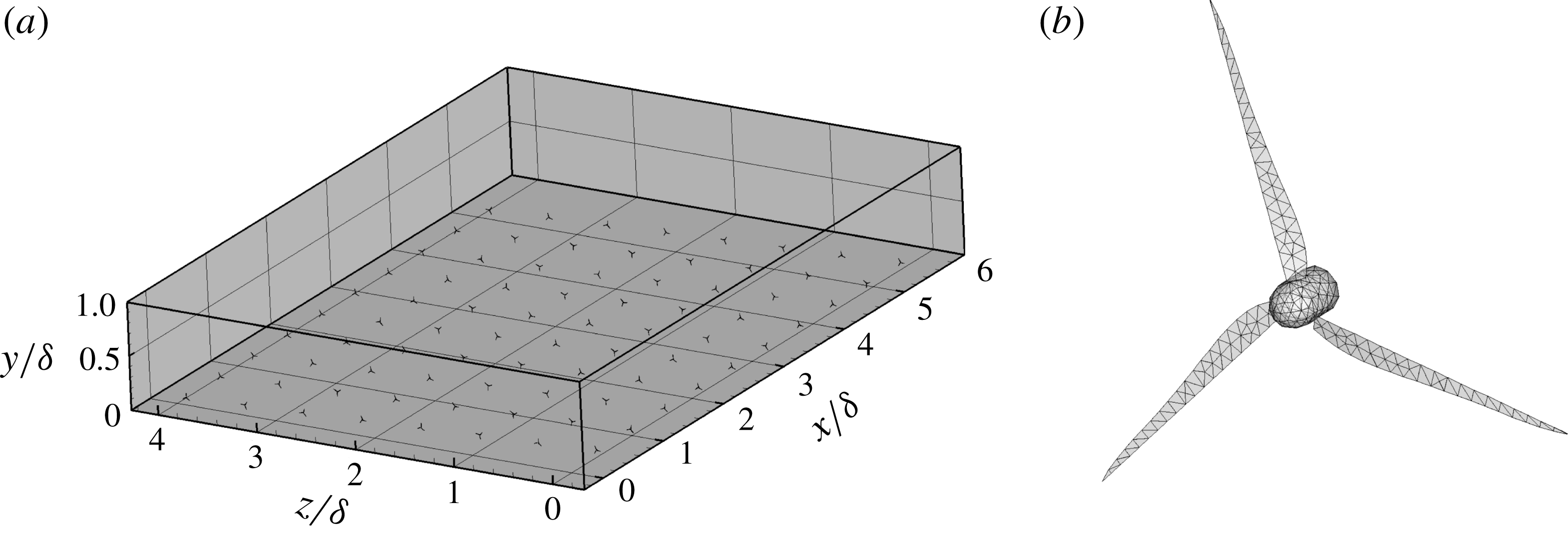
from their respective upwind row or neighbouring column. Figure 1(a) shows the layout of the turbines with the incoming wind blowing in the positive
 $x$
direction. This corresponds to the wind direction heading east in the field (Barthelmie et al.
Reference Barthelmie, Rathmann, Frandsen, Hansen, Politis, Prospathopoulos, Rados, Cabezón, Schlez and Phillips2007). This particular case is chosen due to the availability of experimental measurements and due to the compact and stacked arrangement of the turbines, which can be used to provide first insights into the effects of nacelles on the flow dynamics in wind farms. A precursor simulation is carried out to develop inflow conditions corresponding to a fully developed neutral atmospheric boundary layer. In this simulation the boundary layer height is specified and the flow is driven by a pressure gradient ensuring a constant flow rate. The so specified boundary layer height is set to
 $\unicode[STIX]{x1D6FF}=1000~\text{m}$
and the wind speed at the turbine hub height is set to
 $8~\text{m}~\text{s}^{-1}$
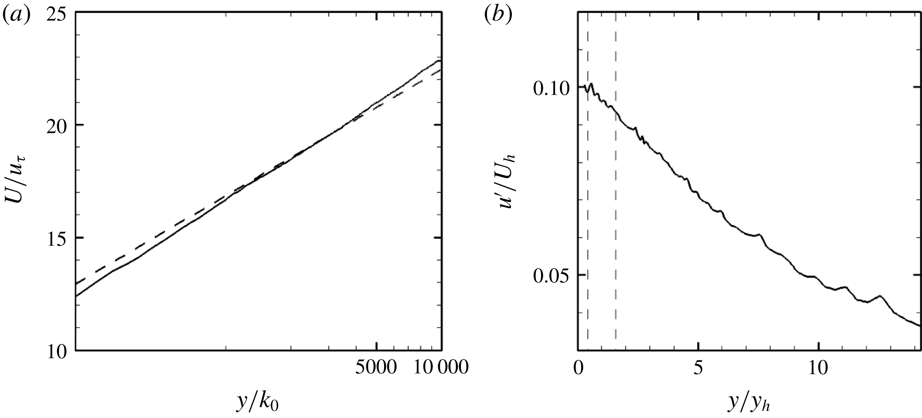
. Instantaneous snapshots of the precursor simulation velocity field are saved and used as inflow for the wind farm simulations. Instantaneous inflow snapshots of sufficient number to ensure statistical convergence of the mean flow are collected to cover the duration of the entire turbine simulation. Figures 2(a) and 2(b) show the statistics of the mean velocity and turbulence intensity of the inflow, respectively. The tip-speed ratio is
 $\unicode[STIX]{x1D706}=\unicode[STIX]{x1D714}R/U_{d}(-1D)=7.5$
for all turbines and is held constant by instantaneously adjusting the angular velocity
 $\unicode[STIX]{x1D714}$
of the turbine blades, where
 $U_{d}(-1D)$
is the rotor disk-averaged downwind velocity at
 $1D$
upwind of each turbine.
(a) Sketch of the Horns Rev wind farm turbine layout with the wind blowing in the positive
 $x$
-direction, and (b) unstructured discretisation of the turbine blades and nacelles for the actuator surface with nacelle model.

(a) Mean downwind velocity normalised by the friction velocity
 $u_{\unicode[STIX]{x1D70F}}$
(solid) with the logarithmic law
 $U/u_{\unicode[STIX]{x1D70F}}=1/\unicode[STIX]{x1D705}\ln (y/k_{0})$
, where
 $\unicode[STIX]{x1D705}=0.4$
(dashed) and (b) turbulence intensity normalised by the hub height velocity
 $U_{h}$
of the inflow. The dashed vertical lines in (b) show the bottom and top tips of the turbine rotor.

The computational domain size is
 $54D\times 12.5D\times 70D$
in the spanwise, vertical and downwind directions, respectively, and is discretised in a Cartesian mesh with
 $1470\times 152\times 1561$
cells in the spanwise, vertical and downwind directions, respectively. The grid size allows for 40 cells per rotor diameter
 $D$
in the turbine region in the spanwise and vertical directions. This grid resolution is finer than other recent studies, such as Porté-Agel et al. (Reference Porté-Agel, Wu, Lu and Conzemius2011), Eriksson et al. (Reference Eriksson, Lindvall, Breton and Ivanell2015), Nilsson et al. (Reference Nilsson, Ivanell, Hansen, Mikkelsen, Sørensen, Breton and Henningson2015) and Wu & Porté-Agel (Reference Wu and Porté-Agel2015) using about
 $D/15$
,
 $D/5$
,
 $D/30$
and
 $D/20$
near rotor resolution, respectively. While the actuator surface model with nacelle requires higher grid resolution compared to standard actuator line and actuator disk models (Yang & Sotiropoulos Reference Yang and Sotiropoulos2018), the required resolution is lower than that required for immersed boundary methods and is well within the range of practical simulations of utility-scale wind farms with present-day computing power (Yang et al.
Reference Yang, Pakula and Sotiropoulos2018). In the downwind direction, the mesh is uniformly distributed with grid spacing approximately equal to
 $D/22$
. According to the actuator surface model of Yang & Sotiropoulos (Reference Yang and Sotiropoulos2018), the turbine blades and the nacelle surface for each turbine are discretised with an unstructured grid as shown in figure 1(b). The chord and twist distributions and lift and drag coefficients for the turbine blades are from Porté-Agel, Wu & Chen (Reference Porté-Agel, Wu and Chen2013). The bottom wall is modelled with the logarithmic law for rough wall with roughness length
 $k_{0}=0.0001~\text{m}$
(Yang et al.
Reference Yang, Sotiropoulos, Conzemius, Wachtler and Strong2015). Free-slip boundary condition is applied at the top and spanwise boundaries.
We carry out two simulations using identical inflow conditions and grid resolution (as described above) and only varying the actuator surface (AS) model (Yang & Sotiropoulos Reference Yang and Sotiropoulos2018) we employ for the turbine structures: (i) case AS-RN, incorporating the actuator surface models both for the rotor blades (R) and nacelle (N); and (ii) case AS-R, incorporating only the rotor blades without the nacelle model. While the turbine tower contributes to wake asymmetry, especially towards the bottom of the wake in wind turbines, observations of an oversized tower (Schümann et al.
Reference Schümann, Pierella and Sætran2013) revealed that the tower wake was not observed in the far wake and less distinguished in the near wake of a wind turbine operating in an upwind wind turbine wake. The effect the tower has on the wake is less in the far wake than the nacelle-induced unstable hub vortex, which has been shown to augment the amplitude of wake meandering several rotor diameters downwind (Kang et al.
Reference Kang, Yang and Sotiropoulos2014; Foti et al.
Reference Foti, Yang, Guala and Sotiropoulos2016). This is especially true in large wind farms due to upwind turbine wake interactions (Schümann et al.
Reference Schümann, Pierella and Sætran2013). Additionally, significantly higher grid resolution would be required to resolve the tower due to its small diameter relative to the turbine rotor size. For that, and because of both the physics-related and computational reasons, the tower geometry is not included in our simulations. The computing time for the nacelle model we employ herein is approximately 2 % of the time for the flow solver (solvers for the momentum and pressure Poisson equations), so including or omitting the nacelle model does not significantly influence the computational time for the same resolution. If an actuator line/disk model is used for the rotor, the computational cost can be reduced by using a coarser mesh similar to simulations in Porté-Agel et al. (Reference Porté-Agel, Wu and Chen2013). However, such simpler models cannot capture the effects of the nacelle vortex instability (Kang et al.
Reference Kang, Yang and Sotiropoulos2014; Yang & Sotiropoulos Reference Yang and Sotiropoulos2018). Three-dimensional instantaneous flow fields are collected approximately every
 $T/11$
(where
 $T$
is the average rotor rotational period of turbines in the first row), stored over 3500 instantaneous flow fields for subsequent analysis.
4 Results
We present and analyse the results of the two wind farm simulations (AS-RN and AS-R) in this section. First, we discuss the mean flow field characteristics in § 4.1. Wake meandering features are analysed in § 4.2. Finally, we discuss the wake meandering expansion and wake expansion in §§ 4.3 and 4.4 and respectively.
4.1 Power output, instantaneous and mean flow field
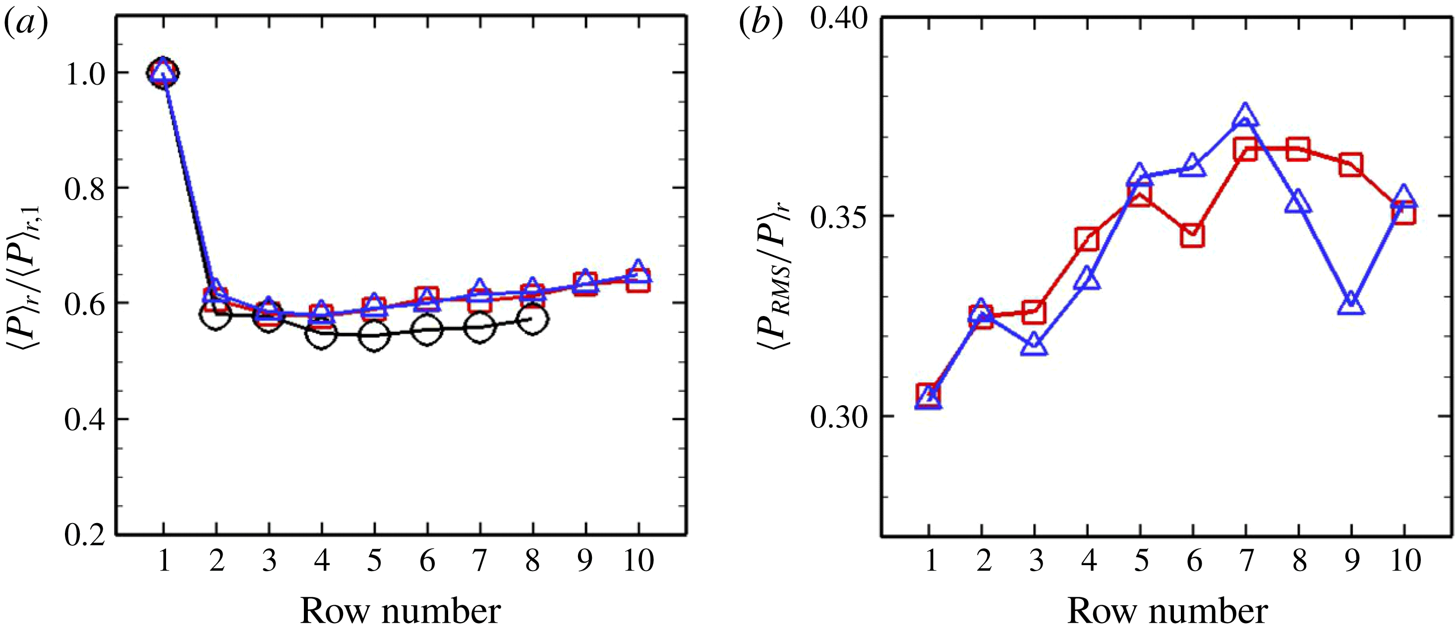
In this section, we start by comparing the row- and time-averaged power and the row-averaged root-mean-square (r.m.s.) of power fluctuations between the two cases, which are calculated by first averaging over time and then over each row. Figure 3(a) compares the calculated row- and time-averaged power
 $\langle P\rangle _{r}$
for both cases, normalised by the power of the first row, where
 $\langle \cdot \rangle _{r}$
indicates row averaging, with the field data obtained from Barthelmie et al. (Reference Barthelmie, Rathmann, Frandsen, Hansen, Politis, Prospathopoulos, Rados, Cabezón, Schlez and Phillips2007, Reference Barthelmie, Hansen, Frandsen, Rathmann, Schepers, Schlez, Phillips, Rados, Zervos and Politis2009). Consistent with the measurements, the first row extracts the most power from the incoming wind and the following rows extract only approximately 60 % of the power of the first row. Both AS-RN and AS-R simulations yield very similar average power per row indicating that the presence of the nacelle model does not have a significant effect on the average power extracted by the wind farm. Figure 3(b) shows the row-averaged r.m.s. of power fluctuations
 $\langle P_{rms}\rangle _{r}$
per row for each simulation. A general trend that the r.m.s. power increases towards an asymptotic maximum of 37 % of the average power is observed for both simulations. However, some differences are observed in that
 $\langle P_{rms}\rangle _{r}$
for the AS-R case exhibit more spatial variability compared to the AS-RN case. The r.m.s. of the fluctuations of the power produced by the entire wind farm is also found to be 3.93 % and 3.33 % for AS-RN and AS-R cases, respectively.
(a) Row- and time-averaged power and (b) row-averaged r.m.s. of power fluctuations per row from measurements (Barthelmie et al. Reference Barthelmie, Rathmann, Frandsen, Hansen, Politis, Prospathopoulos, Rados, Cabezón, Schlez and Phillips2007) (circles) and AS-RN (squares) and AS-R (triangles) cases. It is noted that (b) shows the row-averaged r.m.s. of the power fluctuations from a single turbine instead of the r.m.s. of the fluctuations of the power from a row of turbines.

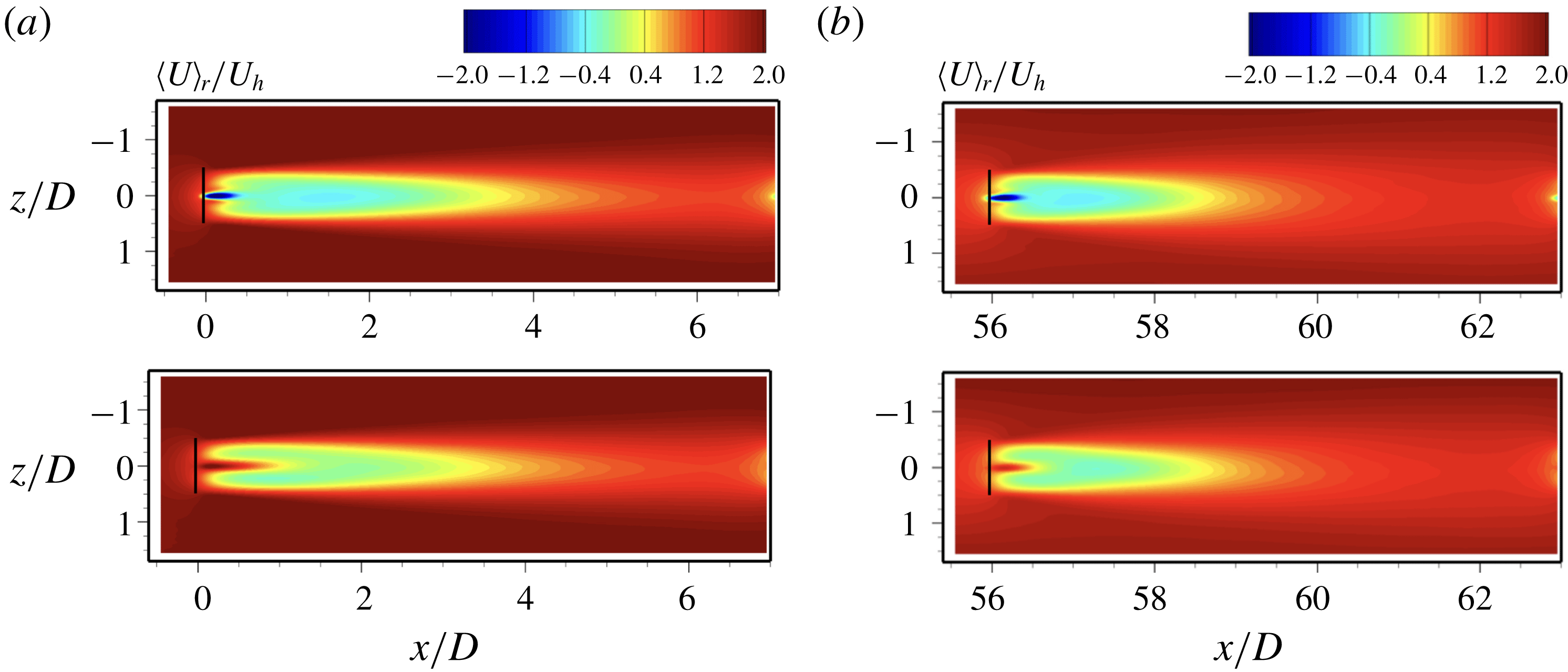
Row- and time-averaged downwind velocity contours,
 $\langle U\rangle _{r}$
, where the upper case letter indicates time averaging and
 $\langle \cdot \rangle _{r}$
indicates row averaging, are shown in figure 4 to illustrate the influence of nacelle model on turbine wake recovery in the first row (a) and the last row (b), respectively. In the AS-RN simulation we see the development of inner wakes that forms directly behind the nacelles, and the outer wake that forms over the extent of the entire rotor disk. We refer to Kang et al. (Reference Kang, Yang and Sotiropoulos2014) and Foti et al. (Reference Foti, Yang, Guala and Sotiropoulos2016) for more details on the interaction between the inner wake and the outer wake. In both rows, the effect of nacelles in the near wakes is observed as a strong inner wake that forms behind the nacelles in the AS-RN simulation. While on the other hand, the AS-R simulation reveals that there is a strong unphysical centreline jet due to the absence of the nacelles. However, in both rows, there is little difference in the average downwind velocity in the AS-RN and AS-R simulations at downwind distances
 $x/D>3$
. This is consistent with the mean turbine power results that showed little difference between the AS-RN and AS-R cases (see figure 3
a). Figure 4 also shows the differences in the mean wake between the first and last rows. It is seen that the wake recovery is slower and the wake width is slightly narrower in the first row than in the last row.
Contours of the row- and time-averaged downwind velocity,
 $\langle U\rangle _{r}$
, for (a) the first row and (b) the last row in the horizontal plane at the hub height. The top and bottom figures are for cases AS-RN and AS-R, respectively.

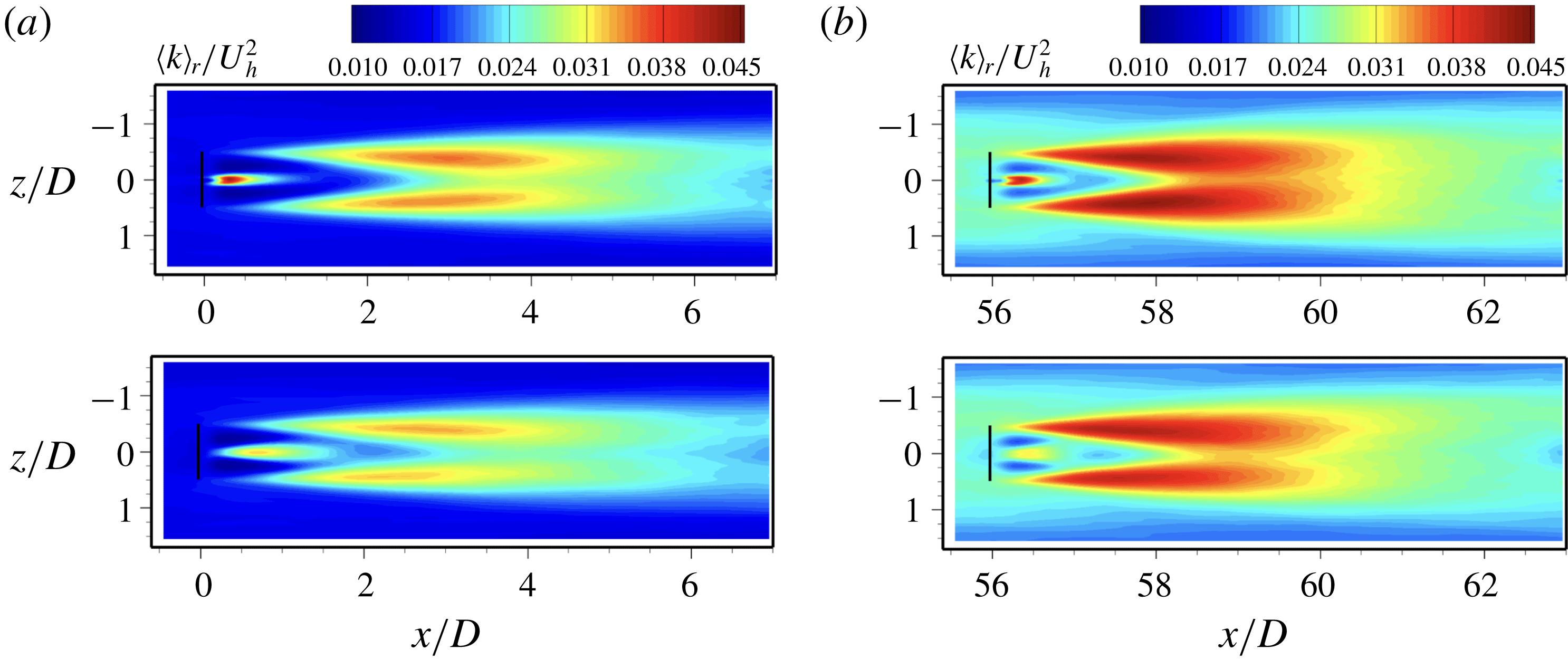
Contours of the row-averaged TKE,
 $\langle k\rangle _{r}$
, for (a) the first row and (b) the last row at the hub height. The top and bottom figures are for cases AS-RN and AS-R, respectively.

Row-averaged turbulence kinetic energy (TKE) contours,
 $\langle k\rangle _{r}$
, are shown in figure 5, which reveal the influence of nacelles on the variation of TKE for turbine wakes in the first row (a) and the last row (b), respectively. It is seen that the nacelles have a significant effect on the TKE at both near and far wake locations, where the TKE from the simulation with the nacelle model (AS-RN) is higher than the simulation without the nacelle model (AS-R) – this result is consistent with the earlier findings of Kang et al. (Reference Kang, Yang and Sotiropoulos2014) for the wake of single turbine. The presence of the nacelles in the AS-RN case produces higher TKE right behind the nacelles in the inner wakes while the TKE is lower in the same location for the AS-R simulation where the unphysical jet is formed. As observed in Kang et al. (Reference Kang, Yang and Sotiropoulos2014) and Foti et al. (Reference Foti, Yang, Guala and Sotiropoulos2016), the inner wake expands outwards intercepting the outer wake (rotor tip shear layer). At
 $x/D=2$
, the inner wake interacts with the outer wake and produces high levels of TKE. The simulation with the nacelles, AS-RN, produces higher levels of TKE after
 $x/D=2$
compared with the AS-R simulation indicating that the nacelles have an effect on the turbulence intensity far downwind of the turbine. However, the location of the maximum TKE in the wake for both simulations is around
 $x/D=3$
. Significant differences in the TKE levels are observed in the last row where the TKE in the downwind wake is higher due to the higher levels of incoming TKE in the upwind turbine wakes.
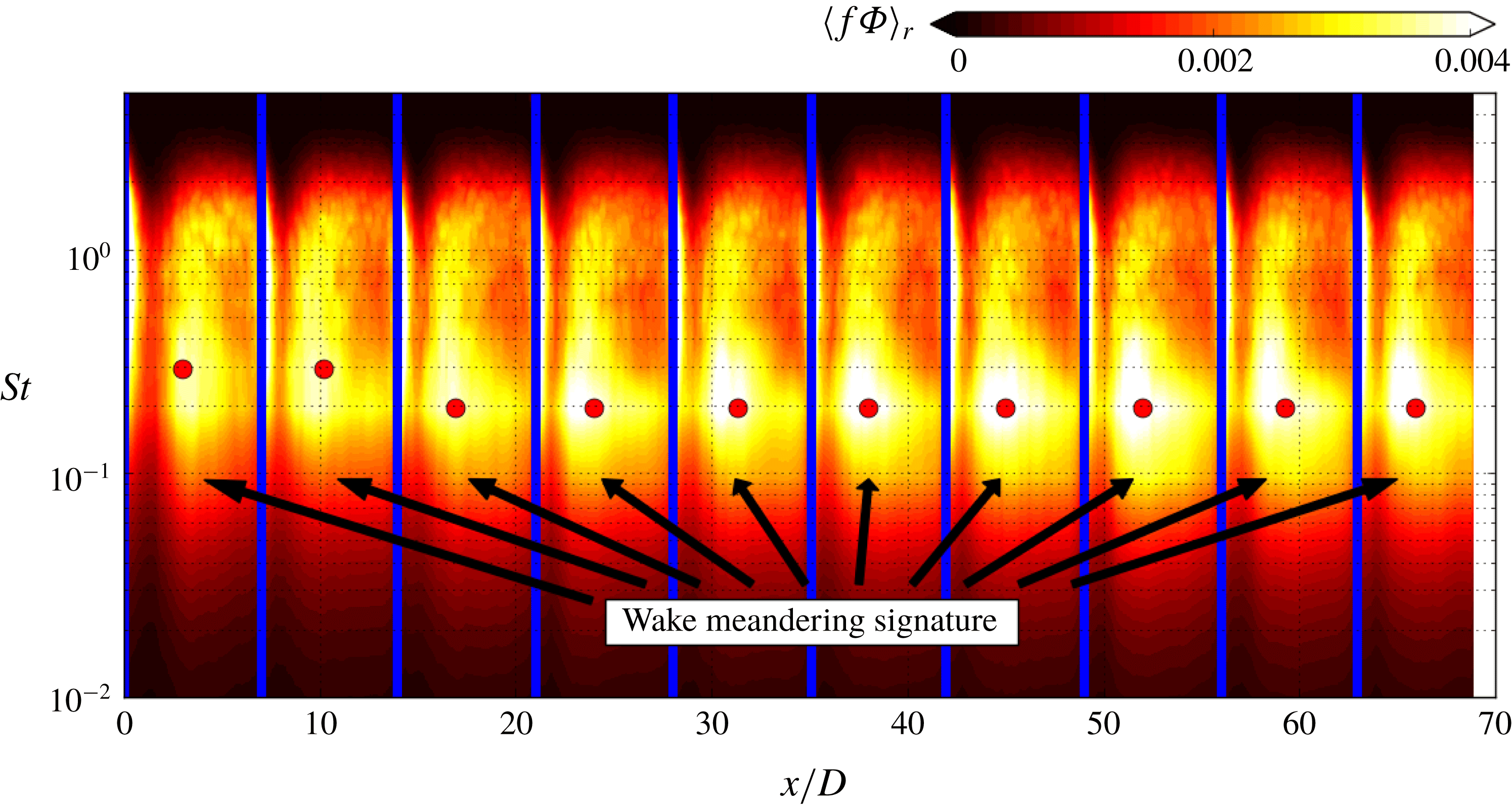
Contours of the row-averaged Fourier power spectral density of the downwind component of the velocity fluctuations pre-multiplied by frequency,
 $\langle f\unicode[STIX]{x1D6F7}\rangle _{r}$
, as a function of the normalised downwind distance,
 $x/D$
, and Strouhal number,
 $St=fD/U_{h_{1}}$
, at hub height
 $y=y_{h}$
for the AS-RN simulation. Vertical blue lines delineate the axial location of each wind turbine. Annotations refer to the region of high PSD that is associated with wake meandering and the circles mark the maximum PSD in the wake meandering region in each corresponding turbine.

4.2 Wake meandering statistics
Motivated by the differences in the TKE distributions of the AS-RN and AS-R turbine wakes, we proceed in this section to investigate the statistics of wake meandering. First, we assess the frequency of wake meandering within the wind farm through the Fourier power spectrum analysis of the downwind component of the velocity fluctuations pre-multiplied by frequency,
 $f\unicode[STIX]{x1D6F7}$
. Figure 6 shows the contours of the power spectral density (PSD) for the AS-RN simulation as a function of the downwind distance
 $x/D$
and Strouhal number
 $St=fD/U_{h_{1}}$
, where
 $U_{h_{1}}$
is the average free-stream downwind velocity at hub height for the first turbine row. The PSD is calculated by extracting time series of data at the hub height and at the time interval of
 $T/11$
for the duration of the simulation at every grid node in the downwind direction (1561 nodes) through the centre of the column of wind turbines. Finally, the PSD is averaged over the turbine wakes in each row (the same downwind distance from each turbine in each row). Downwind of each turbine there are several regions of high PSD that occur at Strouhal numbers greater than unity. These are attributed to the rotor rotating frequencies that persist downwind (this is not very obvious in the near wake where the nacelle wake dominates and for which the dominant frequency is much lower). At Strouhal numbers less than unity there is a region of high PSD that develops approximately
 $3D$
downwind of each turbine and persists for several rotor diameters until the next downwind turbine. This region behind each turbine spanning,
 $0.1<St<0.3$
, is the signature of wake meandering in spectral space. In figure 6 circles mark the maximum PSD in the wake meandering region, which shows a decrease in the meandering associated Strouhal number from the first row to the third row. Moreover, we see that the downwind extent of the wake meandering region and the strength of the PSD associated with meandering frequency increases from the first row to the fifth row suggesting that wake meandering experiences an increase in energy in the first several rows of the wind farm. This energy increase is consistent with the increase in TKE and power fluctuations described above.
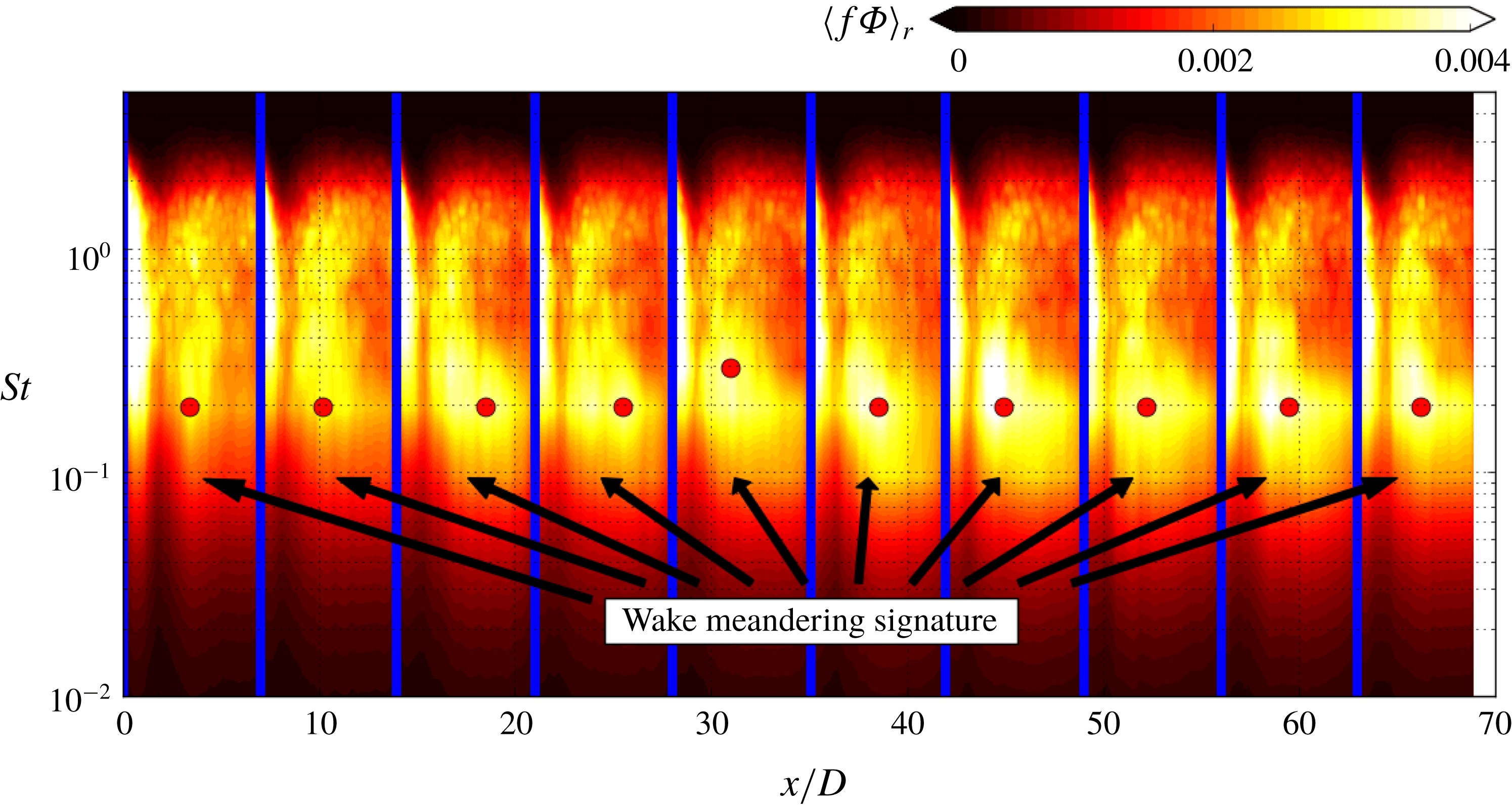
To assess the effect of nacelle-induced coherent structures on wake meandering dynamics, we show in figure 7 the contours of the pre-multiplied PSD in the
 $St-x$
space for the AS-R simulation. Comparing figures 6 and 7 we can see that in both simulations the peak wake meandering frequencies in each row are in the same range of
 $0.1<St<0.3$
. The peak Strouhal number decreases from the first row to the third row in the AS-RN case, while the peak Strouhal number remains nearly constant. The most significant difference between the AS-RN and AS-R simulations is the magnitude of the PSD in the wake meandering region. The contour levels in the wake meandering region in figure 7 are clearly lower than those in figure 6, indicating that the amount of energy in wake meandering is considerably less in the AS-R simulation. This further suggests that the helical coherent structures induced by the nacelles energise the wake meandering.
See figure 6 for caption. The AS-R case is shown here.

To further elucidate the statistics of the wake meandering within the wind farm, we construct the meander profiles behind all the turbines for each simulation. Similar to the previous work of Foti et al. (Reference Foti, Yang, Guala and Sotiropoulos2016), the three-dimensional spatio-temporal meander profiles are obtained from instantaneous velocity fields by employing a three-step process. We recognise that a temporally and spatially evolving flow field
 $\boldsymbol{u}(\boldsymbol{x},t)$
(bold indicates a vector quantity) can be rewritten in terms of its triple decomposition as follows:
 $$\begin{eqnarray}\boldsymbol{u}(\boldsymbol{x},t)=\boldsymbol{U}(\boldsymbol{x})+\boldsymbol{u}_{c}(\boldsymbol{x},t)+\boldsymbol{u}_{i}(\boldsymbol{x},t),\end{eqnarray}$$
where
 $\boldsymbol{U}(\boldsymbol{x})$
is time averaged, a strictly spatial term,
 $\boldsymbol{u}_{c}(\boldsymbol{x},t)$
is the coherent term and
 $\boldsymbol{u}_{i}(\boldsymbol{x},t)$
is the incoherent term (Hussain Reference Hussain1986). In order to obtain a flow field, a filtering procedure is employed to remove random fluctuations from the flow. A coherent time scale
 $\unicode[STIX]{x1D70F}_{c}$
for wake meandering is calculated in the wake of each turbine (as described in Foti et al.
Reference Foti, Yang, Guala and Sotiropoulos2016) and is found to be similar to the turbines numerically studied by Foti et al. (Reference Foti, Yang, Guala and Sotiropoulos2016, Reference Foti, Yang and Sotiropoulos2018b
),
 $\unicode[STIX]{x1D70F}_{c}=0.7T$
. The filtered velocity field:
 $$\begin{eqnarray}\widetilde{\boldsymbol{u}}(\boldsymbol{x},t)=\boldsymbol{U}(\boldsymbol{x})+\boldsymbol{u}_{c}(\boldsymbol{x},t)\end{eqnarray}$$
is first calculated using finite-time interval average, employing fluctuation analysis and the central limit theorem (Chrisohoides & Sotiropoulos Reference Chrisohoides and Sotiropoulos2003), over the coherent time scale of the velocity field throughout the duration of the simulation as follows:
 $$\begin{eqnarray}\widetilde{\boldsymbol{u}}(\boldsymbol{x},t)=\frac{1}{\unicode[STIX]{x1D70F}_{c}}\int _{t-\unicode[STIX]{x1D70F}_{c}/2}^{t+\unicode[STIX]{x1D70F}_{c}/2}\boldsymbol{u}(\boldsymbol{x},t^{\prime })\,\text{d}t^{\prime }.\end{eqnarray}$$
Next, the downwind velocity minima, which track the location of the wake meandering centreline, are obtained in the wake of each turbine. A bounding box in the radial direction around each turbine is employed to limit the velocity minima search to only the wake of that turbine. Finally, a continuous meander profile is created through a low-bypass spatial filtering with a filter width of
 $D/2$
. For details the reader is referred to Foti et al. (Reference Foti, Yang, Guala and Sotiropoulos2016).
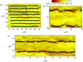
Figure 8 shows three different views of the downwind velocity and the meander profiles projected onto the horizontal plane behind each turbine for the AS-RN simulation at one time instance. Turbine–wake interactions are observed as the wakes from upwind turbines directly interact with downwind turbines. Figure 8 clearly shows that wakes undergo meandering, which may cause turbine power fluctuations due to its inherent unsteadiness. In fact, we see that the power fluctuations as shown in figure 3(b) increase with downwind distance, which provides evidence that upwind turbine wakes affect the power fluctuation levels of downwind turbines. The effects of upwind turbine wakes seem to become saturated around row 6 where the power fluctuations begin to reach a near steady value. The full-view figure shows the overall pattern of the meander profiles at this time instance. From the zoomed-in figures, we can see that the meander profiles remain fairly straight in the first row, but fluctuate wildly for rows deep in the wind farm. From the zoomed-in figures, we can also observe how the meander profiles affect the downwind turbines: (i) the downwind turbine experiences higher incoming velocity when the incoming meander profile (at the velocity minima) is displaced laterally outside the location of the downwind turbine rotor; (ii) the downwind turbine experiences a low incoming velocity when the meander profile directly intersects the downwind turbine. Over a period of time, we can reason that the inherent unsteadiness of the wake meandering from upwind turbines increases the turbulence intensity and causes power fluctuations and dynamic loads for the downwind turbines. In what follows, we proceed to use the meander profiles to investigate how the presence of the nacelles affects the dynamics of wake meandering.
Computed meander profiles (black line) of the instantaneous downwind velocity at hub height of AS-RN simulation (zoomed-in figures on (b) and (c)). The turbine blade locations are shown in green.

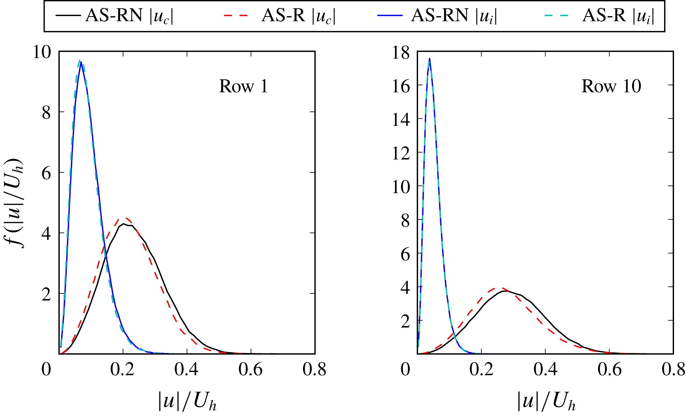
First, we show how the nacelle-induced unstable hub vortex contributes to the coherent and incoherent motions in the wake by comparing in figure 9 the probability density functions (PDFs) of the coherent and incoherent velocity magnitude. The coherent and incoherent velocity magnitude is selected only along the paths of the meander profile behind each turbine for the first row and the last row. As seen, the probability is larger for high coherent velocity magnitude for the AS-RN case compared to the AS-R case. This quantitatively indicates that additional energy is augmented to coherent structures in wake meandering by the unstable hub vortex. The PDFs of the incoherent velocities, on the other hand, are very similar for the simulations with and without the nacelle model.
The PDF of the coherent
 $f(|u_{c}|/U_{h})$
and incoherent
 $f(|u_{i}|/U_{h})$
velocity magnitude normalised by the hub height velocity
 $U_{h}$
using the velocity along the meander profile at each time instance for both the AS-RN (solid) and AS-R (dashed) cases. The PDFs of the coherent velocity magnitude for the AS-RN and AS-R cases are a black line and a red line, respectively. The PDFs of the incoherent velocity magnitude for the AS-RN and AS-R cases are a blue line and cyan line, respectively.

Amplitudes and wavelengths of the meander profiles, derived by projecting the three-dimensional meandering profiles onto the two-dimensional hub height plane to obtain a wave-like form, are used to interpret the coherent motions and the dynamics of the instantaneous wake. The amplitudes of a meander profile are determined by the distance from the centre of the wave-like meander profile to the spanwise extrema. Similarly, wavelengths of the meander profile are captured by calculating the distance between two successive maxima or minima. In Foti et al. (Reference Foti, Yang and Sotiropoulos2018b
) the average amplitude of the meander profile for a single turbine was shown to be scaled by a characteristic length scale
 $L_{T}$
, which is given by
 $$\begin{eqnarray}L_{T}=(T/\unicode[STIX]{x1D70C}\unicode[STIX]{x03C0}R^{2})^{1/2}/f_{m},\end{eqnarray}$$
where
 $\unicode[STIX]{x1D70C}$
is the air density,
 $R$
is the rotor radius and
 $T$
is the thrust on each turbine, which is defined as
 $T=\unicode[STIX]{x1D70C}C_{T}\unicode[STIX]{x03C0}R^{2}U_{h}^{2}/2$
and depends on the thrust coefficient
 $C_{T}$
. The meandering frequency
 $f_{m}=St_{m}D/U_{h}$
, where
 $St_{m}$
is the Strouhal number of wake meandering, is calculated directly from the power density spectra of each wind turbine wake as shown in figures 6 and 7 for both the AS-RN and AS-R cases, respectively, using the incoming velocity associated with each turbine. It is important to note that the Strouhal number range used in figures 6 and 7 is based on the average free-stream velocity for the first turbine row. The dominant Strouhal numbers for wake meandering
 $St_{m}$
are in the range of 0.17–0.25. This range of Strouhal numbers is consistent with a number of studies (Okulov & Sørensen Reference Okulov and Sørensen2007; Medici & Alfredsson Reference Medici and Alfredsson2008; Chamorro et al.
Reference Chamorro, Hill, Morton, Ellis, Arndt and Sotiropoulos2013; Okulov et al.
Reference Okulov, Naumov, Mikkelsen, Kabardin and Sørensen2014; Howard et al.
Reference Howard, Singh, Sotiropoulos and Guala2015; Foti et al.
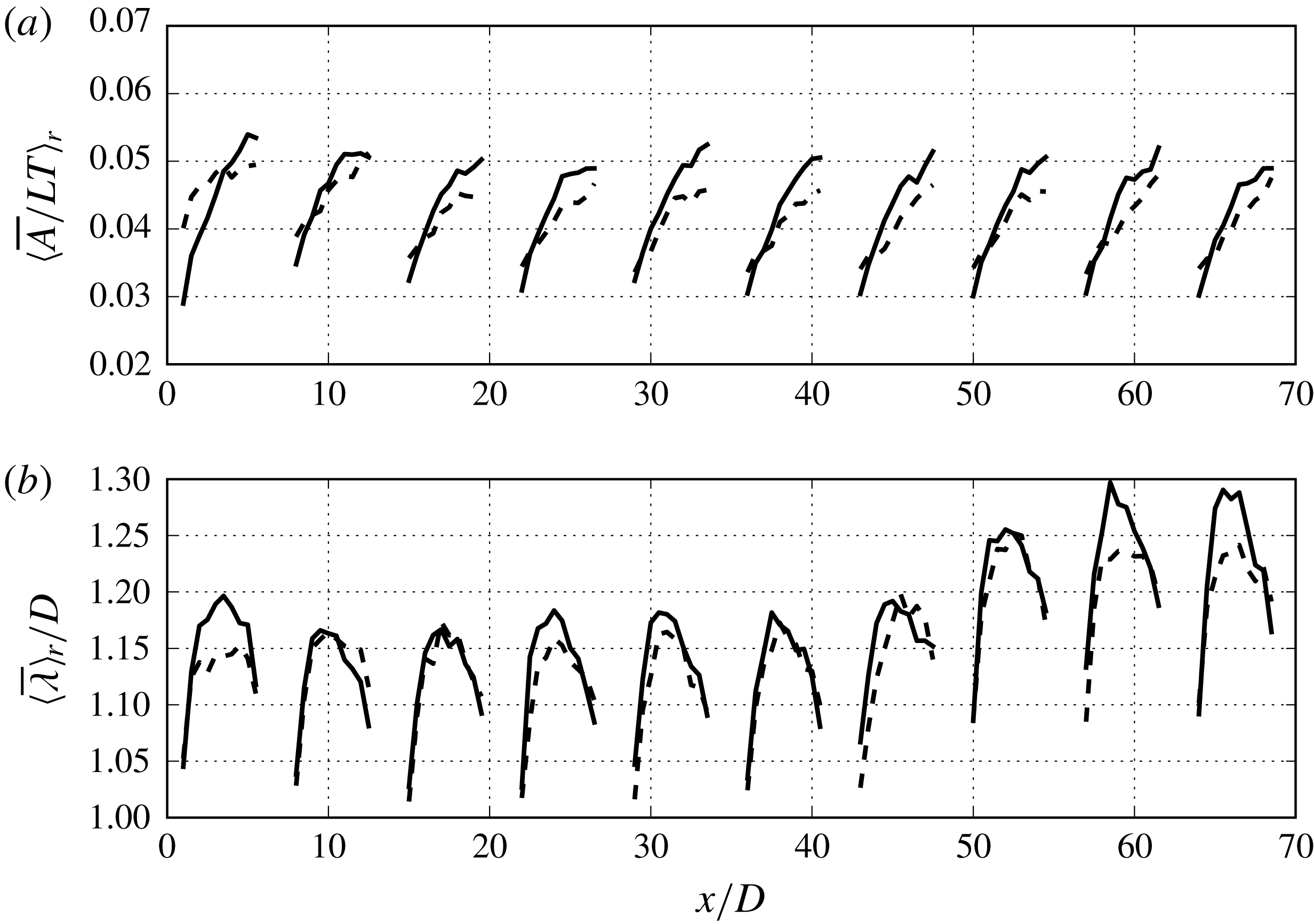
Reference Foti, Yang, Guala and Sotiropoulos2016). Figure 10(a) shows the row-averaged amplitude normalised by
 $L_{T}$
for each row of the wind farm in AS-RN and AS-R. With this scaling, we observe trends where the AS-RN case produces larger amplitudes compared to the AS-R case. The higher amplitude is attributed to the unstable hub vortex that forms behind the nacelle in the inner wake and interacts with the outer wake as explained in Kang et al. (Reference Kang, Yang and Sotiropoulos2014) and Foti et al. (Reference Foti, Yang, Guala and Sotiropoulos2016). The manifestation of the increased wake meandering amplitude in the turbulence statistics is the higher TKE in the wake at
 $x/D=3$
for the AS-RN case compared to the AS-R case. However, the peak amplitudes do not increase as the row number increases, suggesting that within a wind turbine array the
 $L_{T}$
meandering length scale can account for some wind farm interactions. Comparing the average amplitudes in figure 10(a) to single turbine cases described in Foti et al. (Reference Foti, Yang and Sotiropoulos2018b
), we find that the average amplitudes for each row have similar magnitudes. The row-averaged wavelength normalised by the rotor diameter
 $D$
is shown in figure 10(b). The wavelengths of wake meandering increase to over the size of the diameter. Larger wavelengths for the simulation with the nacelle model, AS-RN, compared to the AS-R case are observed. For each row around the distance of
 $4D$
behind the turbine the wavelength starts to decrease, which can be partly attributed to the blockage effect of the downwind turbine. The last three rows have a larger wavelength, especially the final row, where there is no downwind turbine to affect the downwind growth of the meandering. However, we observe a slight decrease in wavelength in the final row, as well.
Comparison of (a) average wake meandering amplitude
 $\langle \overline{A}\rangle _{r}$
normalised by the characteristic length scale
 $L_{T}$
(4.4) and (b) average wavelength
 $\langle \overline{\unicode[STIX]{x1D706}}\rangle _{r}/D$
of wake meandering normalised by the rotor diameter
 $D$
between AS-RN (solid line) and AS-R (dashed line) simulations.

4.3 Analysis of wake expansion using wake meandering statistics
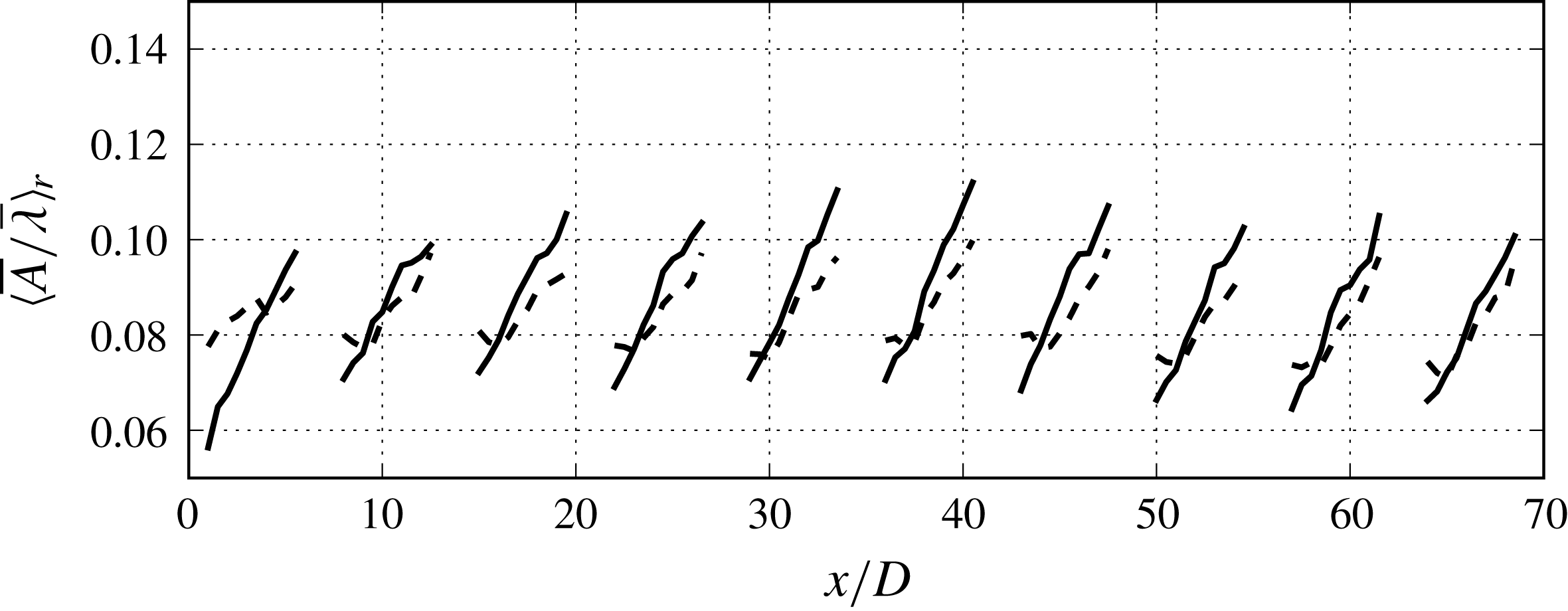
In this section, we explore the expansion and area of influence of the turbine wakes in the wind farm using wake meandering statistics in order to further elucidate the effects of wake meandering on the dynamics of the wind farm and the role that nacelle-induced coherent structures play in determining such dynamics. By understanding the dynamics of the expansion of wake meandering, we hope to gain insights that will enable strategies for control power fluctuations and turbine loading and optimising wind farm layout. Figure 11 shows the row-averaged ratio of the average meander amplitude to the average meander wavelength
 $\langle \overline{A}/\overline{\unicode[STIX]{x1D706}}\rangle _{r}$
, also called the
 $A{-}\unicode[STIX]{x1D706}$
ratio, for each row in both the AS-RN and AS-R cases. The ratio of the amplitude to the wavelength is employed to demonstrate and quantify the dynamic growth of the wake meandering and the expansion of the wake. The quantity is assumed to be a surrogate for the ratio of the transverse to downwind growth of wake meandering. As shown in figure 11, the profiles of the
 $A{-}\unicode[STIX]{x1D706}$
ratio in each row are nearly linear in the region
 $3<x/D<7$
downwind of each turbine monotonically increasing with distance from the turbine. However, the linearity of the
 $A{-}\unicode[STIX]{x1D706}$
ratio is not readily observable from figure 10(a,b) as both the average amplitude and wavelength cease to grow after
 $x/D>6$
for each turbine row, which is partly attributed to the presence of the next turbine row. The
 $A{-}\unicode[STIX]{x1D706}$
ratio indicates that with increasing distance from the turbine, the meander amplitude increases with respect to the wavelength, and that the wake meandering area of influence, i.e. the area bounded by average maximum spanwise extent of the meander profiles behind the turbine, also expands. Figure 11 also reveals some differences between rows, such as the maximum
 $A{-}\unicode[STIX]{x1D706}$
ratio achieved behind each turbine. The sixth row has the maximum
 $A{-}\unicode[STIX]{x1D706}$
ratio, which corresponds to the row of saturation of the power fluctuations and TKE in the wake. Moreover, the slope of the
 $A{-}\unicode[STIX]{x1D706}$
ratio is lower for the AS-R case compared to the AS-RN case.
Ratio of average wake meandering amplitude to average wake meandering wavelength
 $\langle \overline{A}/\overline{\unicode[STIX]{x1D706}}\rangle _{r}$
in AS-RN (solid) and AS-R (dashed) cases.

The
 $A{-}\unicode[STIX]{x1D706}$
ratio can be further investigated through linear regression over the linear range of the profile to obtain two parameters: the slope
 $c_{1}$
and intercept
 $c_{2}$
. The linearity of the
 $A{-}\unicode[STIX]{x1D706}$
ratio leads to the following equation (we remove
 $_{r}$
for clarity):
 $$\begin{eqnarray}\frac{\langle \overline{A}\rangle (x^{\ast })}{D}=c_{1}x^{\ast }\frac{\langle \overline{\unicode[STIX]{x1D706}}\rangle (x^{\ast })}{D}+c_{2}\frac{\langle \overline{\unicode[STIX]{x1D706}}\rangle (x^{\ast })}{D},\end{eqnarray}$$
where
 $x^{\ast }=(x-x_{t})$
is the downwind distance from the turbine location
 $x_{t}$
, and
 $\overline{A}$
and
 $\overline{\unicode[STIX]{x1D706}}$
are both functions of
 $x^{\ast }$
. The row-averaged slope of the
 $A{-}\unicode[STIX]{x1D706}$
ratio
 $c_{1}$
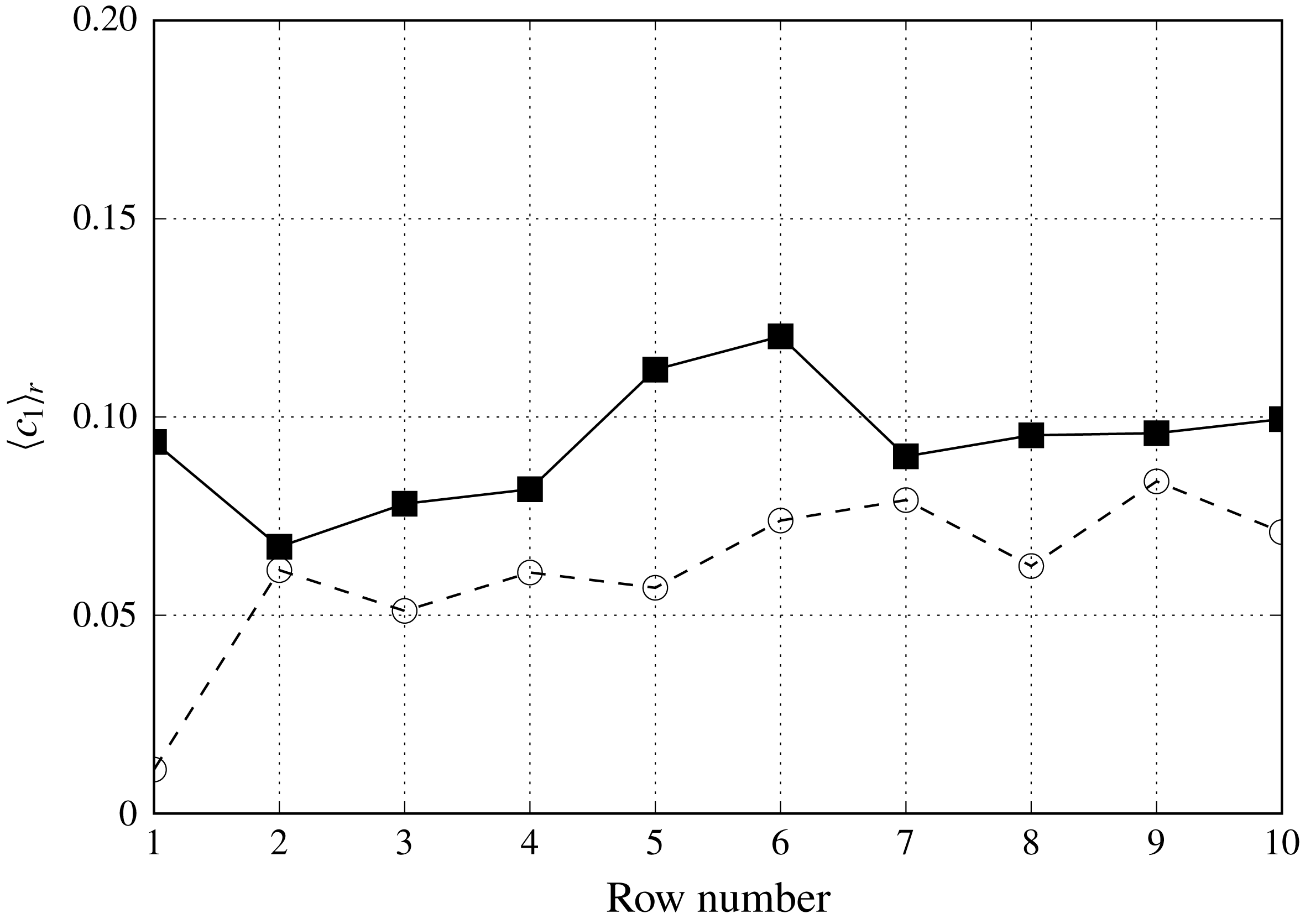
is shown in figure 12 to quantify how the
 $A{-}\unicode[STIX]{x1D706}$
ratio grows for each row. Overall, the slopes of the
 $A{-}\unicode[STIX]{x1D706}$
ratio from the AS-RN case are higher than those from the AS-R case simulation. This further suggests that the nacelle-induced coherent structures affect wake meandering and augment the turbulence intensity, which increases the expansion or spanwise extent of the wake meandering. While the first rows between the two test cases show a significant difference, there is generally a 10 to 50 % difference between the wake meandering expansion.
Coefficient
 $\langle c_{1}\rangle _{r}$
(4.5), slope of average wake meandering amplitude to average wake meandering wavelength averaged over each row, in the AS-RN (solid) and AS-R (dashed) cases.

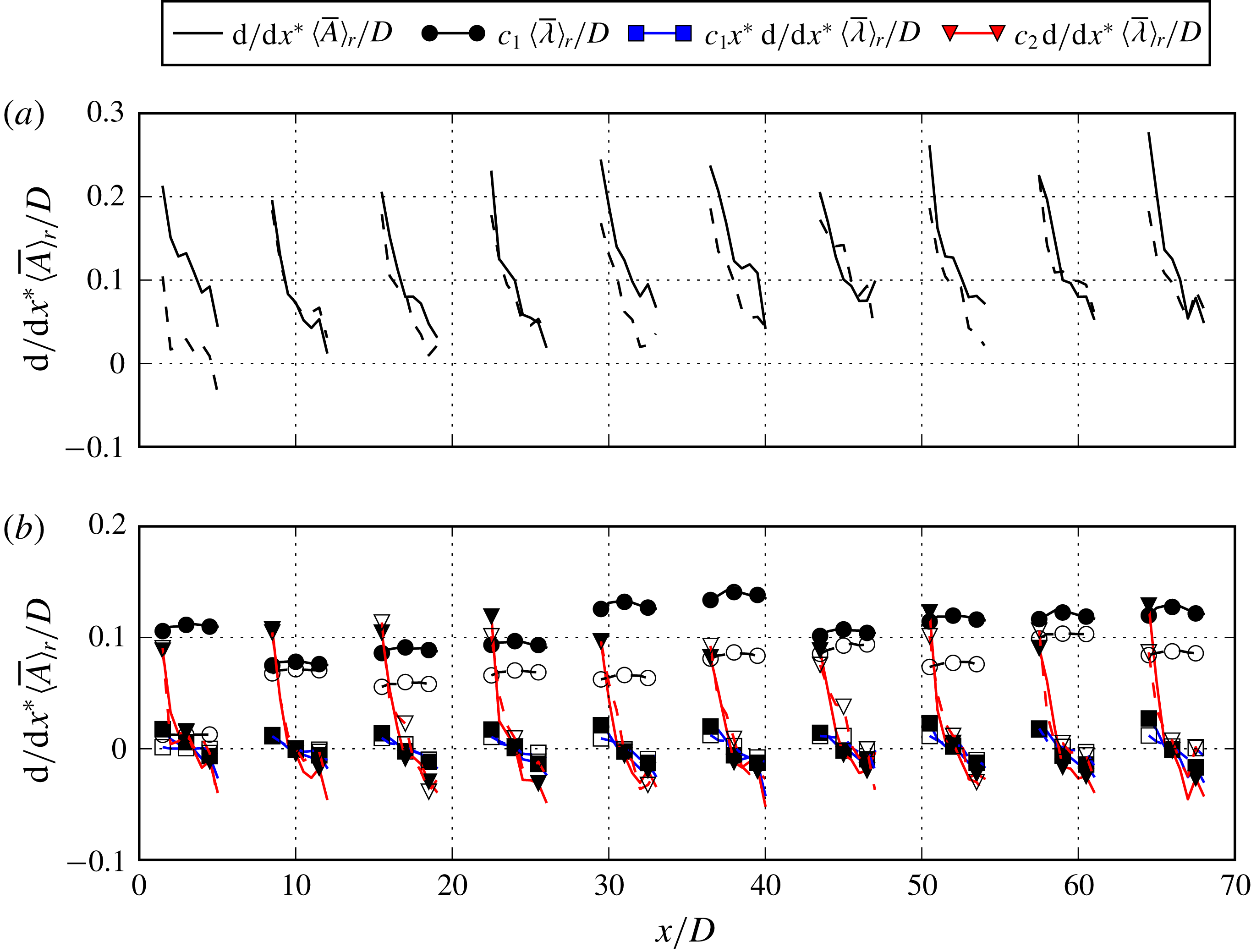
The growth rate of wake meander is defined by taking the derivative of the amplitude in (4.5) with respect to the downwind distance
 $x^{\ast }$
from the turbine as shown in the following (we remove
 $_{r}$
for clarity):
 $$\begin{eqnarray}\frac{\text{d}}{\text{d}x^{\ast }}\frac{\langle \overline{A}\rangle (x^{\ast })}{D}=c_{1}\frac{\langle \overline{\unicode[STIX]{x1D706}}\rangle (x^{\ast })}{D}+c_{1}x^{\ast }\frac{\text{d}}{\text{d}x^{\ast }}\frac{\langle \overline{\unicode[STIX]{x1D706}}\rangle (x^{\ast })}{D}+c_{2}\frac{\text{d}}{\text{d}x^{\ast }}\frac{\langle \overline{\unicode[STIX]{x1D706}}\rangle (x^{\ast })}{D}.\end{eqnarray}$$
The growth rate of wake meandering is comprised of three terms: the mean wavelength, the product of the downwind distance and gradient of the mean wavelength and the gradient of the mean wavelength. Figure 13(a) shows the downwind variations of wake meander growth rate. While the wake meander growth rate is positive, indicating meander growth throughout the wind farm, in general the wake meander growth rate decreases with the downwind distance. The positive wake meander growth rate also indicates that the turbine downwind area influenced by the wake meandering increases with downwind distance. The turbines in the downwind row, as suggested above, create a blockage stunting the expansion of the wake meandering. Moreover, the presence of the nacelles effectively increases the growth of the amplitude and wake meandering.
The individual terms of the growth rate of wake meandering in (4.6) are shown in figure 13(b) in order to assess which term has the largest effect and how to relate the growth rate to physical observations in the wake. It is seen that the wavelength term (the first term on the right-hand side of (4.6)) has the largest effect at all turbine downwind locations. The effect of this term is relatively constant throughout the wake and shows a significant dependence on the nacelle model. This term indicates that a portion of the growth rate of wake meandering is directly proportional to the wavelength, which has been shown to scale with the diameter of the wind turbine (Foti et al. Reference Foti, Yang and Sotiropoulos2018b ). The last two terms in (4.6) show the influence of the spatial gradient of the wavelength on wake meandering expansion. The third term on the right-hand side of (4.6) is observed to have large positive effect in the near wake where significant wake expansion happens, decreasing with downwind distance and having negative effect for further downwind locations. The second term follows a similar trend as the third term, however, with a significantly less influence on the magnitude. Overall, we see that the effect of wavelength (the first term in (4.6)) determines the mean spatial (throughout the wake) growth rate and the effect of the gradient of the wavelength (the third term in (4.6)) determines how the growth rate changes in the downwind direction.
(a) The downwind evolution of the slope of the average amplitude averaged over each row. (b) The downwind evolution of individual contributions to the slope of the amplitude averaged over each row in AS-RN (solid line, filled marker) and AS-R (dashed line, unfilled marker) cases. See (4.6) for definition of various terms.

4.4 Analysis of the wake expansion using velocity deficits
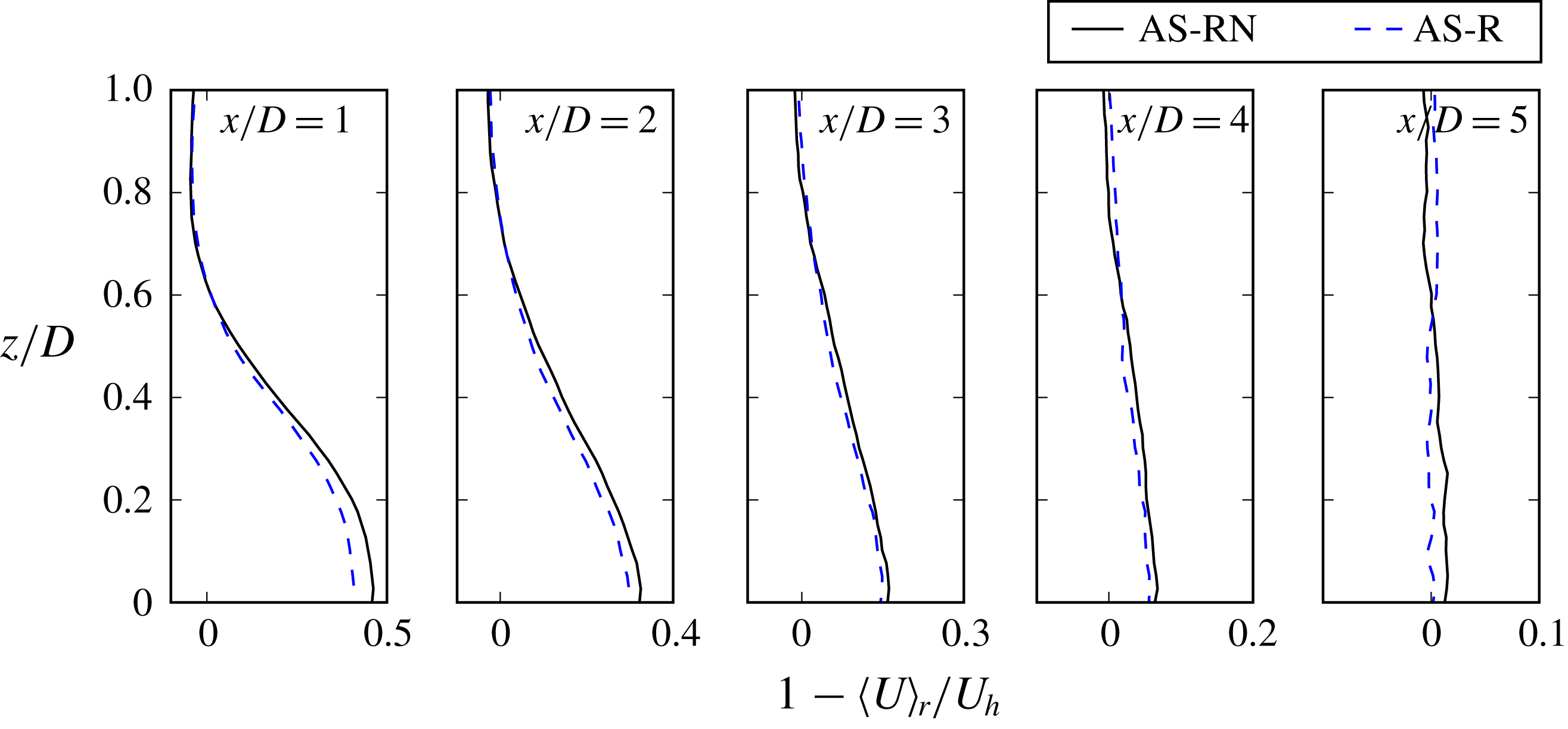
In the previous section we quantified the wake expansion and the wake meandering influenced area in terms of the growth rate of wake meandering amplitudes. In this section we explore three other metrics to quantify wake expansions for comparison to our wake meandering statistics. Figure 14 shows several row- and time-averaged velocity deficit profiles for the sixth row plotted on the horizontal plane at hub height. The profiles indicate that there is a difference in the velocity deficit between the AS-RN and AS-R cases suggesting that the nacelles-induced coherent structures affect the wake recovery, even in the mean sense. The profiles also show that the expansion of the wakes are slightly different. In what follows, we discuss the metrics for calculating wake growth rates to quantify wake expansion.
Profiles of the row- and time-averaged windwise velocity deficit
 $1-\langle U\rangle _{r}/U_{h}$
for row 6 turbines on the hub height plane at
 $x/D=1$
, 2, 3, 4 and 5.

Some previous studies have sought methods to define and track the wakes behind wind turbines (mostly in the mean sense) by using quantities such as mid-point of the wake (Jiménez, Crespo & Migoya Reference Jiménez, Crespo and Migoya2010), centre of mass (Howland et al.
Reference Howland, Bossuyt, Martínez-Tossas, Meyers and Meneveau2016) and Gaussian modelling (Trujillo et al.
Reference Trujillo, Bingöl, Larsen, Mann and Kühn2011; Fleming et al.
Reference Fleming, Gebraad, Lee, van Wingerden, Johnson, Churchfield, Michalakes, Spalart and Moriarty2014). The last method employs fitting a Gaussian-like profile to the wake profiles as a function of downwind distance. We use a similar method in order to quantify the expansion of the wake. However, as with the construction of wake meandering, the time-resolved instantaneous flow field is too noisy to perform an accurate fit. For that, we employ the previously discussed finite-time interval averaging of the wake over the wake coherent time scale to acquire the filtered flow field
 $\widetilde{\boldsymbol{u}}$
as defined by (4.2) to identify coherent wake features.
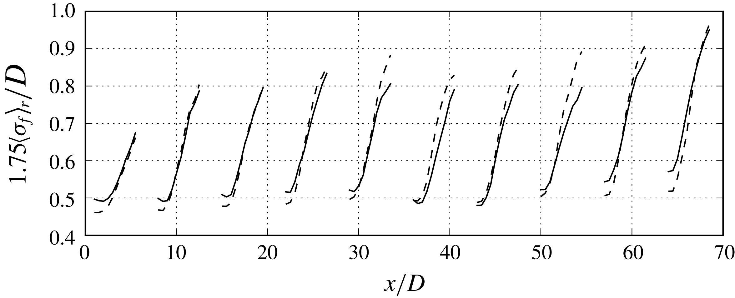
Downwind evolution of the average of the wake radius parameter
 $\langle \unicode[STIX]{x1D70E}_{f}\rangle _{r}$
normalised by
 $D$
for each row for the AS-RN (solid) and AS-R (dashed) cases.

By filtering the flow field, we are able to remove the incoherent velocity fluctuations from the wake while still retaining the qualities of the meandering wake, such as the off-centre location of the velocity minima. The filtered windwise velocity deficit, or turbine-added filtered velocity, which is computed by subtracting the filtered windwise velocity one diameter upwind of the turbine on the hub height plane, is fitted to the following equation:
 $$\begin{eqnarray}\widetilde{u}(x,z)-\widetilde{u}(-D,z)=\frac{B}{2\unicode[STIX]{x03C0}\unicode[STIX]{x1D70E}_{f}}\exp \left(-\frac{(x-\unicode[STIX]{x1D707}_{f})^{2}}{2\unicode[STIX]{x1D70E}_{f}^{2}}\right),\end{eqnarray}$$
where
 $B$
is the amplitude of the Gaussian curve,
 $\unicode[STIX]{x1D70E}_{f}$
is the filtered wake radius parameter and
 $\unicode[STIX]{x1D707}_{f}$
is the centre of the Gaussian curve. The optimal solution to these three parameters is sought with a curve fitting procedure. The curve fit is applied at downwind locations behind each turbine, where
 $\unicode[STIX]{x1D707}_{f}$
is given an initial guess of the velocity minimum location from the previous section. In this analysis, we intend to use the wake radius trends provided by the
 $\unicode[STIX]{x1D70E}_{f}$
, the fitted filtered wake radius parameter, to quantify the wake radius at time scales and length scales comparable to the wake meandering time and length scales. In this sense, we argue that the Gaussian curve fit can be applied to extract such trends.
Figure 15 shows the wake radius parameter
 $\langle \unicode[STIX]{x1D70E}_{f}\rangle _{r}$
averaged with respect to its downwind location and averaged over each row. We scale the wake radius parameter by 1.75 to include 42 % of the data on one side of the mean and in order to correlate it with the defined wake radius at the turbine rotor plane. First, we draw attention to the near wake region where the wake radius parameter is approximately
 $D/2$
, the turbine blade tip location. In order to quantify the wake with the Gaussian fit, we multiply the wake radius parameter by 1.75 such that close to the turbine, the wake radius
 $D/2$
corresponds with the value of the wake radius parameter. This is in agreement with the idea of employing Gaussian statistics to capture the wake because in Gaussian statistics,
 $\unicode[STIX]{x1D70E}_{f}$
is essentially the standard deviation that comprises only 34 % of the data on one side of the mean (centre of the wake).
As shown in figure 15, the downwind evolution of the wake radius parameter increases, nearly linearly, throughout the wake. Around
 $x/D>6$
downwind of each turbine, the growth rate decreases due to the next row of turbines. The maximum wake radius achieved in each wake is dependent on the row. The first row has the smallest wake radius while the growth of the wake increases with the number of rows. For the interior rows, the wake radius increases to approximately 80–90 % of the diameter. Figure 15 also reveals a difference between the wake radius for the AS-RN and AS-R cases. The case without the nacelles shows a marked increase in the wake radius parameter in the far wake locations and across different rows while is lower in the near wake. This is counter to the observation on the downwind variation of wake meander statistics (e.g. figure 10
a), where the meander amplitudes and wavelengths are higher for the AS-RN case.
We also apply the Gaussian curve fitting method to the time-averaged flow field
 $U$
to extract an average wake radius parameter
 $\unicode[STIX]{x1D70E}_{a}$
to provide details on wake expansion in the mean sense. The expansion rate of the wake,
 $\unicode[STIX]{x1D6FC}_{f}$
and
 $\unicode[STIX]{x1D6FC}_{a}$
based on
 $\unicode[STIX]{x1D70E}_{f}$
and
 $\unicode[STIX]{x1D70E}_{a}$
, respectively, can be obtained from the slope of the downwind evolution of the wake width by taking the windwise gradient with respect to the distance from the turbine. Due to the near linearity at
 $x/D>3$
for
 $\langle \unicode[STIX]{x1D70E}_{f}\rangle _{r}$
and at
 $1<x/D<5$
for
 $\langle \unicode[STIX]{x1D70E}_{a}\rangle _{r}$
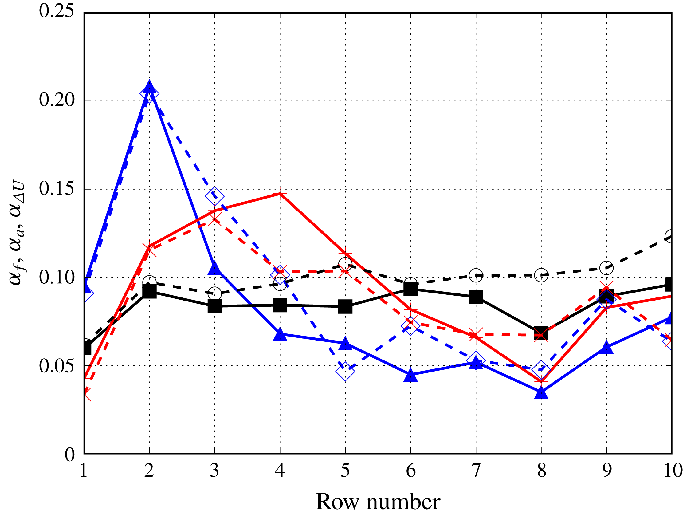
(see figure 15), a single wake expansion rate per turbine can be obtained. Figure 16 shows the wake expansion for both the filtered and average wake radius parameter for both simulated cases. The filtered wake expansion is shown to increase from the first row to the second row and remain relatively constant through the rest of the turbine rows. The wake expansion calculated from the filtered velocity deficits from the AS-RN simulation is less than that from the AS-R case. The wake expansion calculated from the time-averaged velocity deficits is more dependent on the row number compared to the filtered wake expansion. For both simulation cases, the average wake expansion increases from the first row to the fourth row. Then, there is a decrease to a more constant wake expansion after row 6. This result is also consistent with the saturation of wake energy and the onset of a fully developed wind farm regime. The average wake expansion does not show as pronounced difference between the AS-RN and AS-R simulations, but towards the last few rows the wake expansion for the AS-R simulation is higher. We compare these results with the wake meandering expansion rate shown in figure 12 or 13 and see that the expansion magnitude is relatively close. However, the trends of the case with the nacelle model and without the nacelle model are reversed.
Before we discuss the difference between the wake expansion and wake meandering expansion, we consider the wake width and a wake growth rate defined by the turbine-added mean velocity. The wake width using the turbine-added mean velocity is found where
 $U(x,z)-U(-D,z)=-0.01U_{h}$
. The wake growth rate
 $\unicode[STIX]{x1D6FC}_{\unicode[STIX]{x0394}U}$
is then defined as the downwind derivative of the computed wake radius. The growth rate is nearly constant between
 $2<x/D<5$
. The row-averaged growth rates are also shown in figure 16 for each simulation case. The mean velocity wake growth rate increases from the first to the second row and then decreases to a near constant throughout the other rows in the wind farm. In row numbers greater than 3, the turbine-added mean velocity wake recovers before the subsequent row and the growth rate decreases to zeros as detailed in figure 16 for the last row.
The row-averaged wake growth rates
 $\unicode[STIX]{x1D6FC}_{f}$
,
 $\unicode[STIX]{x1D6FC}_{a}$
and
 $\unicode[STIX]{x1D6FC}_{\unicode[STIX]{x0394}U}$
computed using the Gaussian curve fitting on the filtered average velocity deficit profiles, the Gaussian curve fitting on the average velocity deficit profiles and the mean velocity deficit respectively. AS-RN
 $\unicode[STIX]{x1D6FC}_{f}$
(black square), AS-R
 $\unicode[STIX]{x1D6FC}_{f}$
(black circle), AS-RN
 $\unicode[STIX]{x1D6FC}_{a}$
(red plus), AS-R
 $\unicode[STIX]{x1D6FC}_{a}$
(red x), AS-RN
 $\unicode[STIX]{x1D6FC}_{\unicode[STIX]{x0394}U}$
(blue triangle) and AS-R
 $\unicode[STIX]{x1D6FC}_{\unicode[STIX]{x0394}U}$
(blue diamond).

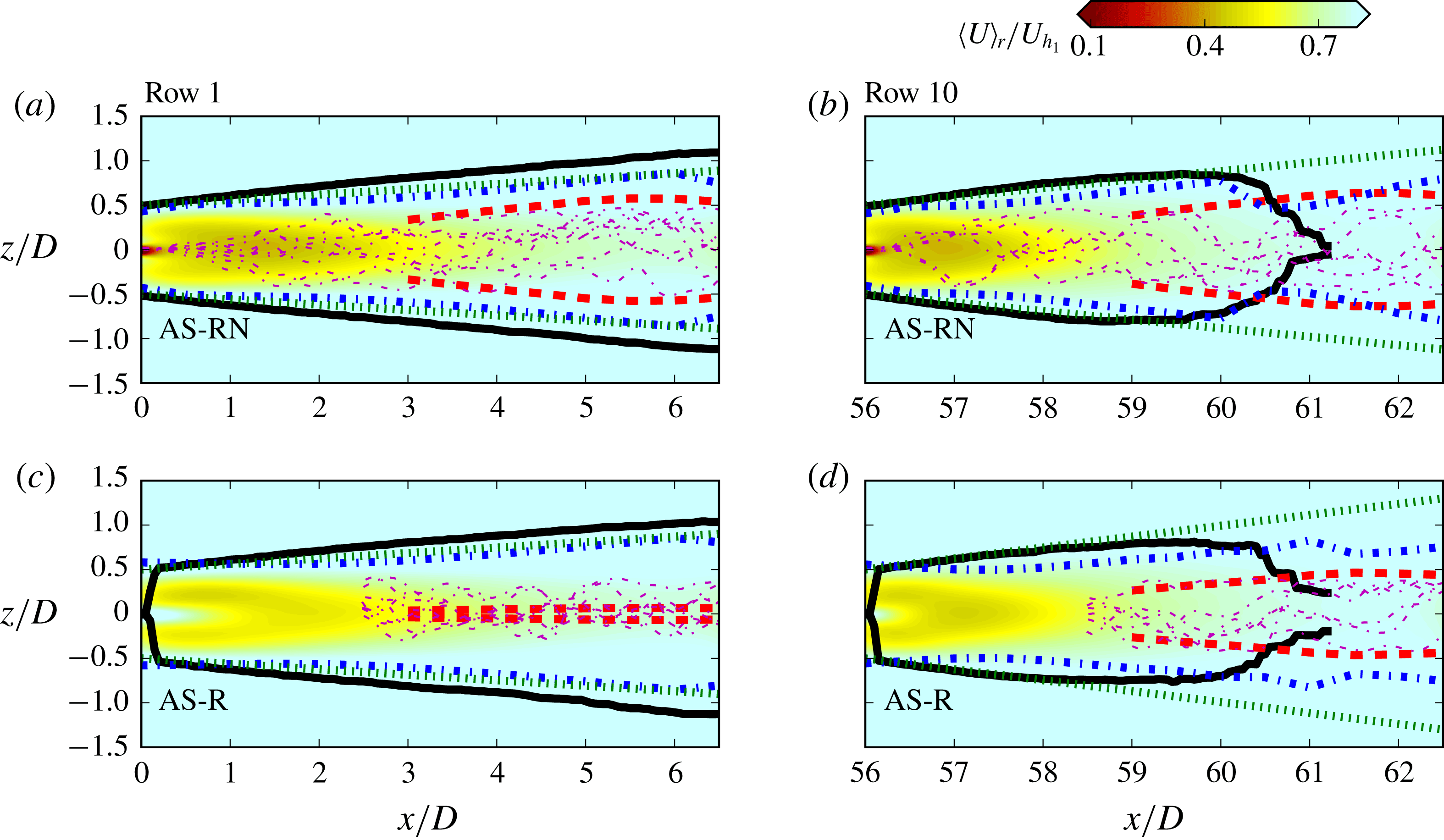
Finally, we compare in figure 17 wake influenced regions computed using the approaches discussed earlier for the first and last row for both simulation cases for the purpose of assessing the role of the nacelle-induced coherent structure in the spanwise expansion of the wake and provide general insights into wind turbine layouts in wind farms. The wake influenced area is defined as the area of the wake between the upper and lower half lines defined by the different wake expansion computation techniques. The growth rate of wake meandering, only quantified from
 $x/D>3$
, has an origin at the centreline of the turbine with the other expansion coefficients defined to have an origin at the turbine tip. These origins are based on how the expansion is defined. The boundary line of the filter wake expansion and average wake expansion are defined by the filtered and average wake radius parameter, respectively, with respect to the downwind distance. The boundary lines for the mean velocity wake growth is determined by the spanwise location where the mean velocity deficit approaches zero.
As shown in figure 17, in the first row for the AS-RN case, the wake area determined by the mean velocity deficit growth rate extends from the turbine blade tip and linearly grows towards the second row. Both the filtered and average wake expansion wake boundaries behave in a similar manner, starting at the turbine blade tip and linearly extending towards the second row. On the other hand, the wake meandering expansion boundaries include the smallest area by increasing linearly and slowly reducing slope towards the second row. We can visualise the significant difference in the wake meandering expansion for the AS-RN and AS-R simulations where the AS-RN wake meandering expansion wake influenced area is larger than that for the AS-R simulation. Instantaneous meander profiles shown in the figure corroborate that wake meandering transverse extent grows with downwind distance faster in the AS-RN case.
The row-averaged wake influenced area based on mean velocity deficit (black, solid), Gaussian fitting to the average wake (green, dotted), Gaussian fitting to the filtered wake (blue, dash-dotted) and the wake meandering area
 $\text{d}(A/D)/\text{d}x^{\ast }$
(red, dashed). Several meander profiles (magenta, dash-dotted) are included for (a,c) the first row and (b,d) the last row. Also plotted are contours of the row-averaged mean downwind velocity normalised by the first row incoming hub height velocity
 $\langle U\rangle _{r}/U_{h_{1}}$
. (a,b) and (c,d) are the cases AS-RN and AS-R, respectively.

While the wake influenced areas are similar for three metrics in the first row, the results for the last row, which are statistically similar for rows 6–10, show that the definition of the wake can greatly affect the computed wake area. The contrasting results are mainly because of the definitions of the wake influenced area in terms of using time-averaged metrics. By using time-averaged velocity statistics (average wake expansion growth rate and mean velocity deficit growth rate), the wake influence area begins to increase from the turbine blade tip and then decreases because the velocity deficit recovers in the mean sense. Moreover, the mean velocity deficit and mean turbine-added velocity in rows 6–10 are lower and higher, respectively, for the AS-R case compared to the same row in the AS-RN case. This causes higher mean growth rates for the AS-R case as demonstrated in figure 16. The lower mean velocity deficit, especially in rows 6–10, in the AS-R case is caused because the upwind wakes recover slower due to lower turbulence mixing and turbulence intensity as shown through the TKE in figure 5. Overall, the higher turbulence intensity in the wakes caused by the nacelle-induced coherent structures enables a faster wake recovery. Recognising this, mean statistics may not be the most suitable metrics to use in order to compare the wake expansions where the wind farm begins to become fully developed.
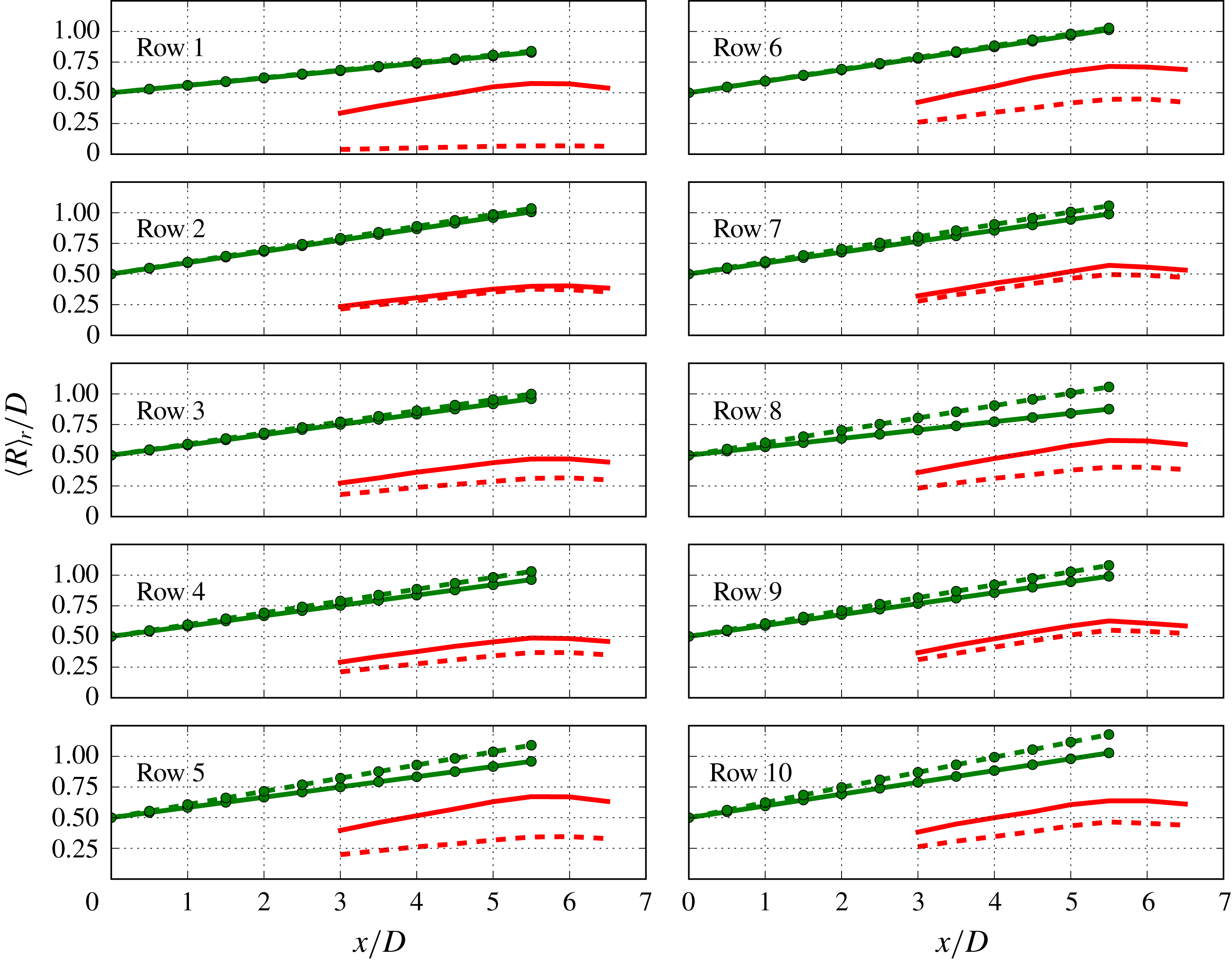
The half-width
 $\langle R\rangle _{r}/D$
normalised by the diameter of the row-averaged wake influenced area based on
 $\text{d}(A/D)/\text{d}x^{\ast }$
(red) and Gaussian fit to the average wake (green circle) for the AS-RN (solid) and AS-R (dashed) cases.

However, both the wake meandering expansion, and to a lesser extent the filtered wake expansion, reveal that the wake has a much larger influenced area when considering statistics at the time scale of wake meandering. The finite-time interval averaging used to extract the coherent velocity for the wake meander profiles integrate the dynamics and instantaneous behaviour of wake meandering indicating the inherent unsteadiness of the wake, which cannot be quantified from the time-averaged wake widths. Quantitatively, figure 18 shows the comparison of the half-width of the wake meandering and average wake expansion influenced areas for rows in both simulations. The differences between the AS-RN and AS-R simulations are clearly visualised with the wake meandering region being larger in the AS-RN simulation. There are subtle differences in the filtered wake expansion between the two simulations where the half-width is slightly higher for the AS-RN case between 1–4
 $D$
downwind. On the other hand in figure 18, the average wake expansion growth rate for the AS-R case in downwind rows is larger than those for the same rows in the AS-RN, which corroborate our observations in figure 17. Overall, by comparing metrics that use the instantaneous behaviour, the dynamics of the wake is elucidated, confirming that the enhanced turbulence intensity caused by the nacelle-induced coherent structure affects the meandering region of the wake. The statistics of the wakes for rows 6–10 discussed in the previous two sections reveal that the wind farm starts to exhibit statistically consistent results for each of those rows. This suggests that starting near or at row 6 the onset of a fully developed state is attained within the wind farm boundary layer.
5 Conclusions
We carried out LES to investigate the effects of wind turbine nacelles on the power output and wake dynamics, especially wake meandering of turbines in a utility-scale offshore wind farm. For both cases, the turbine blades are modelled by an actuator surface blade model. For the case with turbine nacelles, the turbine nacelle is modelled with an actuator surface nacelle model. The actuator surface models for turbine blades and nacelle have shown to account for the effects of the wind turbine nacelle and capture the energetic coherent structures it induces and their impact on far wake meandering. The computed average power from both cases shows good agreement with field measurements. Also, both the simulations with and without the nacelle model produce similar mean downwind velocity fields in the far wake, although the nacelle model correctly captures the emergence of an inner wake for all wind turbines. Differences between the two cases, however, are found in the turbine power fluctuations and turbulence kinetic energy. The presence of the nacelles increases the power fluctuations and turbulence intensities because each nacelle creates a spiralling unstable hub vortex, which precesses slowly, expands radially and ultimately interacts with the rotor tip shear layer (outer wake) several rotor diameters downwind energising and increasing the turbulence intensity levels in the far wake.
The effects of nacelles on the statistics of the wake meandering are investigated using a three-dimensional spatio-temporal reconstruction and spectral analysis. The amplitudes of wake meandering profiles are shown to increase when the nacelle model is employed. The analysis indicates that a previously proposed thrust-based length scale can account for the influence of upwind turbines in wake meandering amplitudes.
Further analysis of the wake expansion using wake meandering statistics reveals that the area influenced by wake meandering grows through the subsequent turbine rows at a higher rate for the case with the nacelle model. On the other hand, the wake influenced areas computed with several other methods employing the mean and filtered velocity deficit profiles are larger for the simulation without the nacelle model. This is mainly because the wake influenced areas computed from the velocity deficit profiles and the wake meandering area defined by the meander profiles describe different aspects of turbine wakes. The former describes the lateral extent of the turbine wakes, while the latter describes the possible locations of turbine wakes, which indicate the turbine wake unsteadiness responsible for the dynamic loads on the downwind turbines. This observation emphasises the importance of including a wake meandering model in reduced-order models (Yang & Sotiropoulos Reference Yang and Sotiropoulos2016; Foti, Yang & Sotiropoulos Reference Foti, Yang and Sotiropoulos2017) in order to improve the prediction of dynamic loads. A curve fitting method using the filtered velocity field indicates that the wake influenced area extends throughout the wake of the turbine while the wake radius computed using the mean velocity flow field reduces in the far wake as the wake behind the turbine recovers.
Our work demonstrates for the first time that the energetic coherent structures induced by the nacelle of each turbine have a significant and measurable effect in the level of turbulence intensities, wake unsteadiness and power fluctuations in large wind farms. Thus, incorporating the nacelle model in turbine parameterisations is critical for accurate predictions of these quantities, which in turn affect the performance of the wind farm and the levelised cost of energy. Accurate prediction of wind farm power fluctuations, for instance, is a critical prerequisite for developing reduced-order models capable of predicting wind farm performance at scales relevant to integrating wind farm output into the power grid – from days to minutes ahead. On the other hand, dynamic loads on turbine structures, which depend on the turbulence levels in the wind farm and affect the life span of wind turbines and the levelised cost of energy, will be underpredicted without accounting for the nacelle-induced coherent structures in the wake of each turbine. Therefore, incorporating a nacelle model in wind farm simulations enables more accurate predictions of wake meandering in wind farms and provides data sets of higher fidelity, which enhance our understanding of turbine wake dynamics and development of improved physics-based low-order wake models for controlling turbine wakes in realistic wind farms. Our work also points to the intriguing possibility of controlling the intensity of far wake meandering, the dynamic loads on turbine structures and wind farm power fluctuations by controlling the flow in the immediate vicinity of the nacelle of each turbine. Exploring such possibilities, however, will be left as topics for future research.
Acknowledgements
This work was supported by US Department of Energy (DE-EE0002980, DE-EE0005482 and DE-AC04-94AL85000), Xcel Energy (RD 4-13 and HE4-3) and Sandia National Laboratories. Computational resources were provided by National Renewable Energy Laboratory, the University of Minnesota Supercomputing Institute and the Institute for Advanced Computational Science at the Stony Brook University.