

Introduction
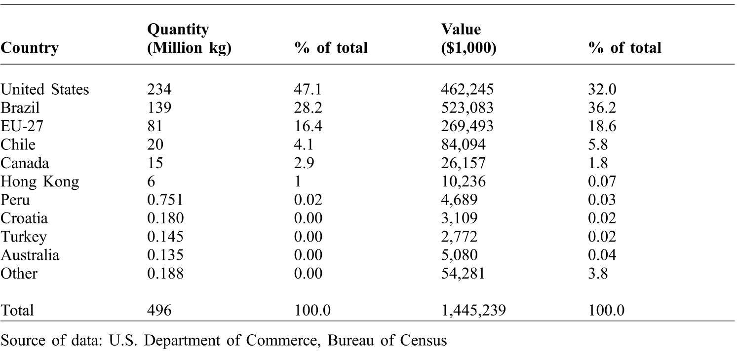
Turkey trade flows have been relatively strong over the last decade although growth has declined slightly due to the global economic recession, which has affected many countries, developing and developed alike. In 1990, world imports of turkey were only 0.194 million metric tons (MMT) turkey, but by 2008 that amount had risen by 148%. The world's consumption of turkey meat is the fourth largest among major animal protein products such as beef (from cattle and not water buffalo or bison), pork, and broilers (USDA-PSD, 2013). Turkey is examined in this study because it is a close substitute for broiler meat, the third fastest growing animal protein product, and it also serves as a substitute for the other animal proteins such as beef and pork. Turkey export data for the world and major exporting countries are reported in Table 1. In 2008, the U.S. was the world's largest exporter of turkey meat, accounting for 47% of the 496 million kilograms (kg) of turkey meat exported worldwide. Brazil was in second place, followed by the European Union - 27(EU-27). About 99% of the world's turkey exports came from the top seven turkey exporters. In addition to the volume of trade, the value of turkey trade has been strong over the last decade. The value of turkey exported by the U.S. was less than it was for Brazil, primarily due to the free trade agreement established with two of its major importers, Mexico and Canada. Brazil captured 36% of the world's total expenditure on exported turkey meat. Export expenditures for EU-27 turkey trade accounted for almost 19% of the world's total.
Major turkey exporters of the world (2008).

Source of data: U.S. Department of Commerce, Bureau of Census
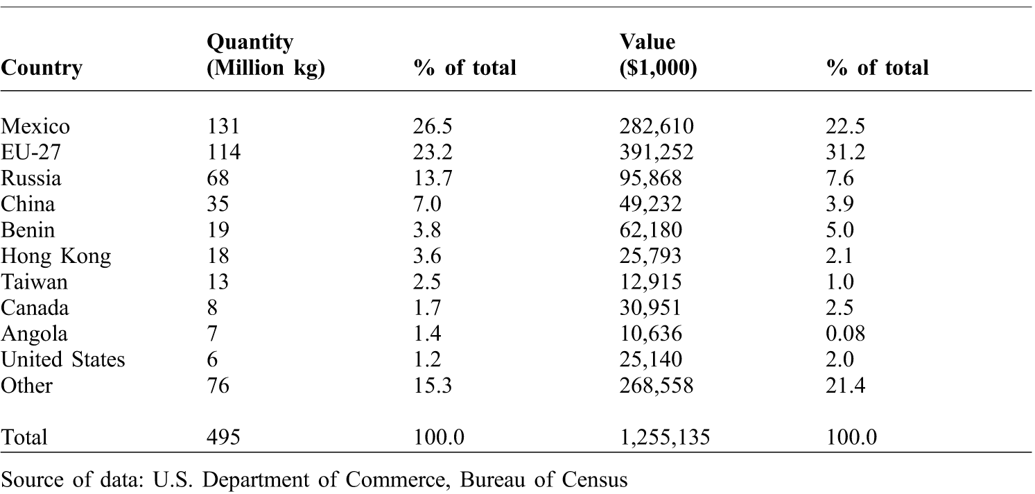
Table 2 shows the world's top 10 turkey import markets for 2008. Mexico was the world's largest importer of turkey meat and continues to lead today. The U.S. is Mexico's primary supplier of turkey meat. Almost 27% of the world's turkey imports were delivered to Mexico. Not far behind was the EU-27, which accounted for 23%. The value of imported turkey was considerably higher for the EU-27 than for Mexico, because over half of the Mexican imported turkey was shipped by the United States as a member of North American Free Trade Agreement (NAFTA).
Major turkey importers of the world (2008).
Source of data: U.S. Department of Commerce, Bureau of Census
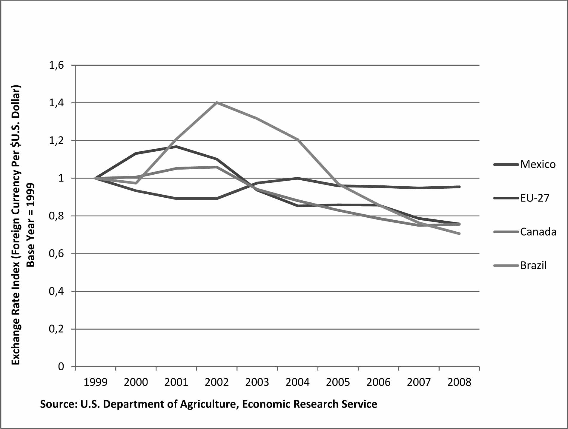
One of the key economic factors that influence international commodity trade is exchange rate volatility. Exchange rate volatility can be defined as the variance associated with price for which the currency of country ‘A’ can be exchanged for country ‘B’ currency. The volatility in exchange rates is important because it helps determine the price that an importing country pays for turkey or any other commodity traded internationally. Exchange rates for major turkey trading countries are reported in Figure 1. In this figure discussion has been limited to foreign currencies relative to the U.S. dollar, although it is also concerned with bilateral volatility between all trading countries. Major changes in the value of the U.S. dollar relative to the currencies of other turkey exporting and importing countries occurred from 1999 to 2008. For example, since 2001, the U.S. dollar has declined 37% relative to the Euro and 28% relative to the Canadian dollar. Since 2002, the dollar lost half its value relative to the Brazilian real. Brazil has shown more volatility relative to the dollar (according to Figure 1) than the other three countries. Mexico is the world's leading turkey importing country and is primarily supplied by the United States. From 1999 to 2008, the Mexican peso has shown the least amount of volatility and its value has appreciated almost 5% relative to the dollar. Over the same period, Mexico's turkey imports from the United States increased 27%.
U.S. Dollar exchange rate indexes for selected countries: 1999-2008
Source: U.S. Department of Agriculture, Economic Research Service
The objective of this study is to evaluate the impact of exchange rate volatility on turkey trade flows for the world. More specifically, this study will determine the short- and long-run effects of exchange rate volatility and assess the impacts of regional relationships on turkey trade flows. While it was expected that the signs to be the same for both short-and long-run exchange rate volatility, intuitively we expect the size of the irrespective impacts to be different.
Previous studies measuring exchange rate volatility
In the early 1970s, currencies of major developed countries were allowed to float and, since that time, a rich body of literature has evolved measuring the impacts of exchange rate fluctuations on international trade. Economists often argued that the risk associated with volatile exchange rates caused international trade to decrease because producers who are very sensitive to risk focus on supplying domestic markets. However, De Grauwe (Reference DE GRAUWE1988) argued that the verdict was still out because theoretical findings suggest that risk adverse producers and firms can benefit from exporting even when exchange rates are volatile. Based on previous empirical studies, there is no concrete consensus on this issue. Klein (Reference KLEIN1990) analysed exports from more than 50 U.S. sectors and discovered that the impacts of exchange rate volatility on the various sectors were insignificant, with four of the sectors having negative coefficients and seven having positive coefficients.
One of the potential problems with previous analyses, as discussed by Anderson and Garcia (Reference ANDERSON and GARCIA1989), is that a number of studies focused on aggregate trade flows, overlooking the fact that the effects of exchange rate volatility may differ by commodity or sector. In agriculture, output decisions are made before exchange rates are realised due to the biological nature of farming and marketing lags involved with final sale transactions. Thus, depending on the commodity type, exchange rate volatility is likely to differ.
While many studies have shown exchange rate volatility to have negative impacts on agricultural trade (Pick, Reference PICK1990; Cho et al., Reference CHO, SHELDON and MCCORRISTON2002; Kandilov, Reference KANDILOV2008), there are some exceptions. Exchange rate volatility had a positive impact on poultry exports from Thailand according to findings by Langley et al. (Reference LANGLEY, GIUGALE, MEYERS and HALLAHAN2000). While analysing Japanese demand for U.S. pork and beef, Miljkovic et al. (Reference MILJKOVIC, MARSH and BRESTER2002) found that the impact of exchange rate volatility on the trade of these products is insignificant. A positive relationship between exchange rate volatility and U.S. poultry exports was noted by Awokuse and Yuan (Reference AWOKUSE and YUAN2006), who also concluded that volatility estimates are sensitive to the chosen volatility measure. Finally, Bonroy et al. (Reference BONROY, GERVAIS and LARUE2007) examined the relationship between exchange rate volatility and Quebec pork exports to the United States and Japan. Employing a multivariate threshold model, a positive relationship between exchange rate volatility and pork exports to the United States was found.
Following Karemera et al. (Reference KAREMERA, MANAGI, REUBEN and SPANN2011), this study makes use of a generalised gravity model to examine how exchange rate volatility affects trade flows. Both short- and long-run exchange rate volatility measures are considered. Panel data are employed which permit examination of the fixed and random effects in addition to factors such as distance, common border, same language, population, national income, and membership in regional trade agreements.
Model specification
In this section, we provide an empirical specification of a gravity model used to identify the determinants of turkey trade flows. The theoretical derivations of the model are widely discussed in the literature. The following model is a standard specification used by Linnemann (Reference LINNEMANN1966), Anderson, (Reference ANDERSON1979), and Bergstrand (Reference BERGSTRAND1985; Reference BERGSTRAND1989); and more recently by Anderson and Van Wincoop (Reference ANDERSON and VAN WINCOOP2003) and Karemera et al. (Reference KAREMERA, MANAGI, REUBEN and SPANN2011). The gravity model used in this study is as follows:
Note that the t subscripts are omitted for convenience.
The variables in equation (1) are defined as follows:
TXij = quantity of turkey imported by country j from country i;
Yi (j)= real gross domestic product in country i(j);
Ni (j)= population in country i(j);
Dij = distance between countries i and j;
Vij = real exchange rate volatility between countries i and j;
NAFTA = 1 if countries i and j are NAFTA partners and 0 otherwise;
APEC = 1 if countries i and j are APEC partners and 0 otherwise;
EU = 1 if countries i and j are EU-27 members and 0 otherwise;
Border = 1 if countries i and j share the same border and 0 otherwise;
Language = 1 if countries i and j speak a common language and 0 otherwise; and
εij is a random error term.
Equation 1 is specified as a generalised gravity equation with free trade variable augmentations. The level of development represented by a country's gross domestic product (GDP) is a key element of the model. The exporter's GDP indicates the country‘s capacity to export turkey and a positive coefficient sign is expected. An increase in the importer's GDP represents an increased domestic purchasing power and a positive sign is expected. Population (N) is a traditional gravitational variable and is included to reflect the exporting country production and export capabilities while it represents the market size of the importing country. Thus, a rise in the exporting and importing countries’ population should be associated with an increase in trade.
The distance and border dummy variables were included as proxies for transportation costs. The distance between countries (Dij) was included under the hypothesis that member countries close to each other are more likely to have similar cultures or cultural heritages, similar patterns of consumption and production, and greater incentives to trade with each other. The common border dummy variable is included in the model because, in addition to characteristics identified for countries within close proximity, it is assumed that there is relatively more trade between countries with common borders than countries geographically separated.
Binary variables representing free trade agreements (FTAs) and regionalisation were included in the gravity models to represent factors aiding or deterring trade. We consider the following agreements for our analysis: NAFTA, EU-27, and APEC. NAFTA represents the North American Free Trade Agreement between Canada, Mexico, and the United States, The EU-27 accounts for the member states of the European Union -27, and APEC represents the Pacific Rim countries that are members of the Asia-Pacific Economic Cooperation.
The effects of exchange rate volatility
Exchange rate risk is expected to influence the level of trade flows between any pair of trade partners. Two measures of exchange rate volatility are considered for the analysis. Let the currency exchange rate between countries i and j at times t and k be denoted as XRij, t. Following Koray and Lastrapes (Reference KORAY and LASTRAPES1989) and Chowdhury (Reference CHOWDHURY1993), short-run exchange rate volatility is measured as a moving standard deviation:
Where m is the order of the moving average.
Second, following Peree and Steinherr (Reference PEREE and STEINHERR1989) and Cho et al. (Reference CHO, SHELDON and MCCORRISTON2002), long- run volatility is specified as:
where max(min) denotes the maximum(minimum) values of the exchange rate within the time period t and XRPij,t is the equilibrium exchange rate. Other terms have been previously defined. Cho et al. (Reference CHO, SHELDON and MCCORRISTON2002) noted that the equilibrium exchange rate is traditionally set to the average rate over the previous period. The value of t has been set to 4 due to a shorter time series. The equilibrium exchange rate was set to the average exchange rate over the moving window to be consistent with the sampled period used in this study.
Data
Turkey trade data for all countries were provided by UN Comtrade, United Nations Statistics Division, for 1999-2008. Real GDP data were obtained from the World Bank, International Monetary Fund, HIS Global Insight, and Oxford Economics Forecasting. Real exchange rates were obtained from USDA's Economic Research Service macroeconomic data set. Population data were provided by the U.S. Census Bureau. The distance between countries was obtained from the website: http://www.distancefromto.net. Several regional impacts were analysed. NAFTA consists of the United States, Canada, and Mexico, and the Asia-Pacific Economic Cooperation (APEC) consists of Australia, Brunei, Canada, Chile, China, Hong Kong, Indonesia, Japan, Malaysia, Mexico, New Zealand, Papua New Guinea, Peru, Philippines, Russia, Singapore, South Korea, Thailand, United States, and Vietnam. The European Union (EU-27) is another region analysed which includes Austria, Belgium, Bulgaria, Cyprus, Czech Republic, Denmark, Estonia, Finland, France, Germany, Greece, Hungary, Ireland, Italy, Latvia, Lithuania, Luxembourg, Malta, Netherlands, Poland, Portugal, Romania, Slovakia, Slovenia, Spain, Sweden and the United Kingdom.
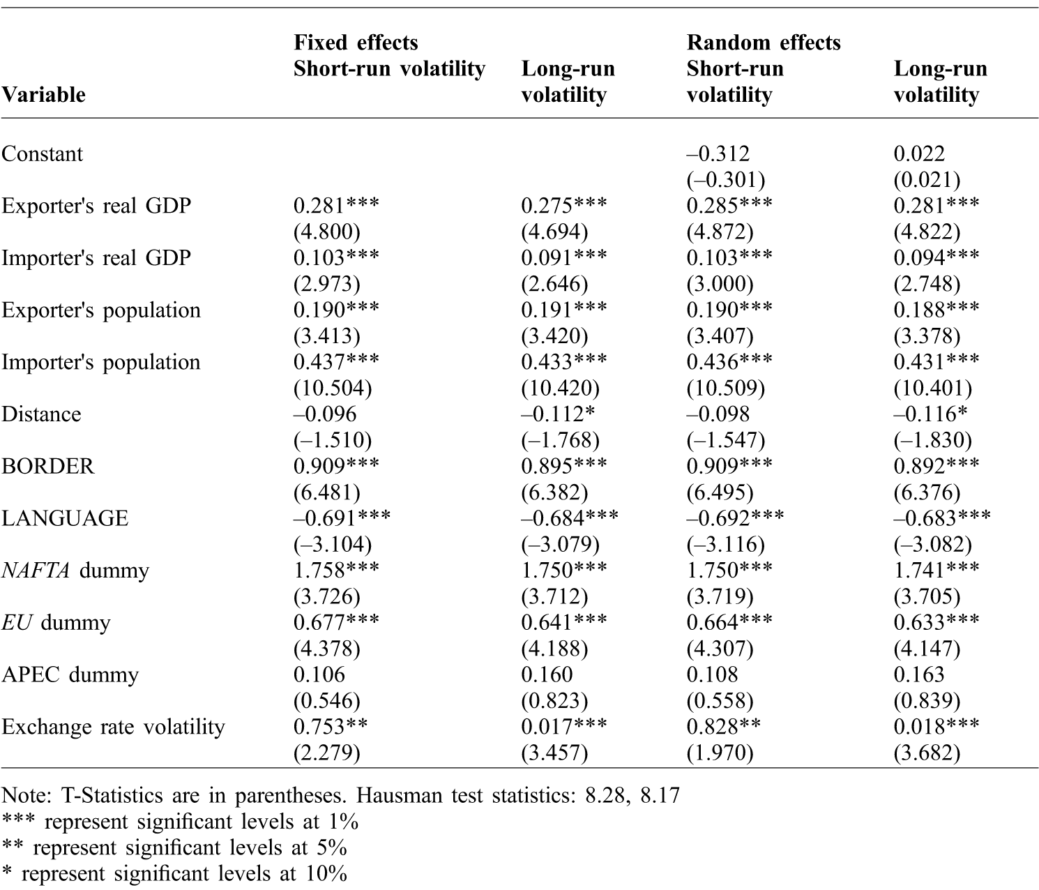
The natural log of equation (1) was derived for all variables except the dummy variables. We then estimated the gravity model using panel data. Each measure of exchange rate volatility was considered separately and the results are reported in Table 3. For convenience, we denote the estimation results using equation (2) as the short-term estimates, and equation (3) as the long-term.
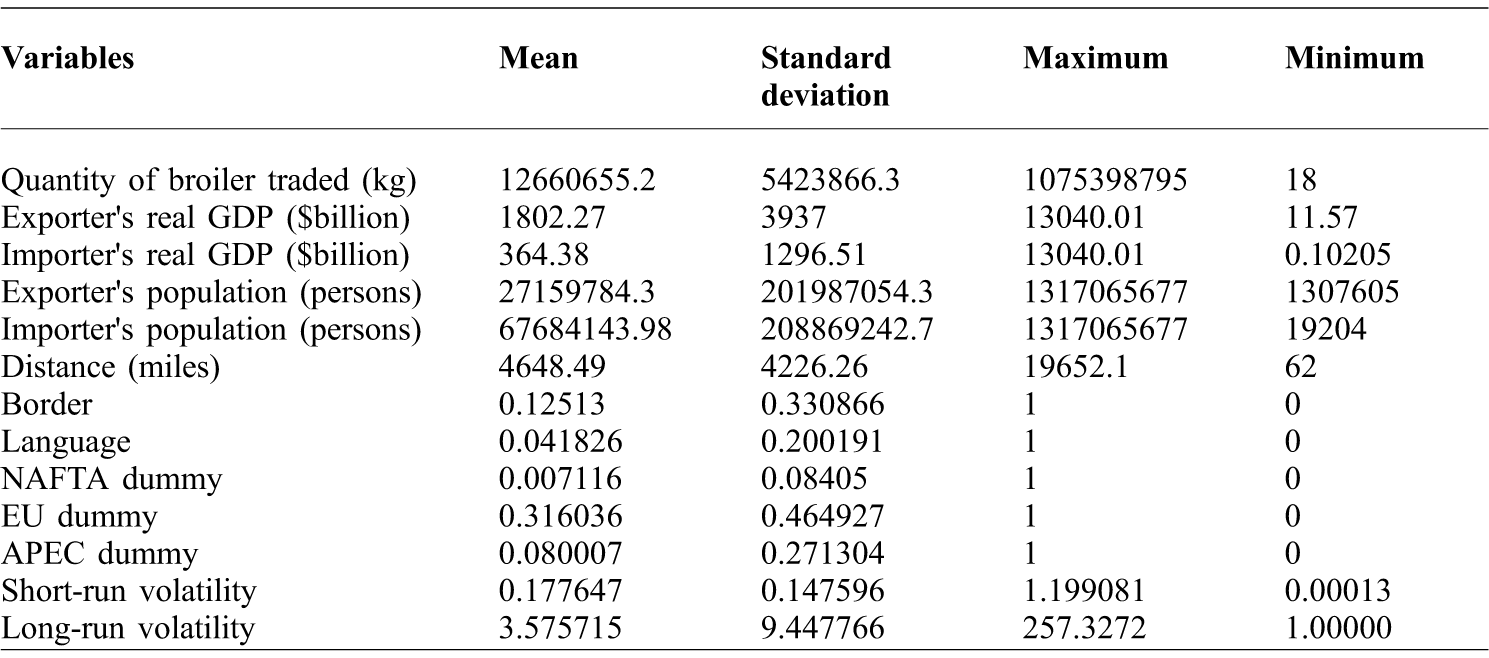
Variable definitions and sample statistics (sample size = 3,132).
Variables summary statistics
All country pairs analysed in the gravity model have positive trade flowsFootnote 1, a procedure used by Sheldon et al. (Reference SHELDON, MISHRA, PICK and THOMPSON2013), Karemera et al. (Reference KAREMERA, MANAGI, REUBEN and SPANN2011; Reference KAREMERA, SMITH, OJAH and COLE1999), and Koo and Karemera (Reference KOO and KAREMERA1991). Countries with incomplete data for more than two years were omitted from the analysis, leaving a total of 271 country pairs, which included the world's top ten exporters and importers of turkey. The variable sample statistics are presented in Table 3. Mexico imported the largest quantity of turkey meat from the U.S. in 2008. Of the many countries involved in turkey trade, the United States had the largest GDP, while China had the largest population. The distance from exporting and importing ports was greatest for trade between Chile and China and shortest between Hong Kong and Macau. Over 14% of the trading partners were neighbouring countries, and 4.8% spoke the same language. Three trading groups were used in the gravity model to highlight trade diversion. Of the three regions, 32% of the turkey meat traded was intra- European Union (27 movements).
Results: the impacts of income and population
Estimates were obtained using the RATS statistical software (Estima, 2009). The estimation results are reported in Table 4, for both the random and fixed effects models. Hausman specification tests show that the random and fixed models produced similar results; thus no comparison will be discussed. Income and population coefficients have the appropriate signs and are significant at the 1% level. Results suggest that a 1% increase in the exporting (importing) country's income would increase turkey meat trade by 0.28% (0.09%) (based on the random effect model and long-run volatility). Considering the magnitude of the estimated GDP coefficients, which are less than unity, results suggest that the quantities of turkey meat traded would increase by less than 1%, given a 1% increase in the importing or exporting country's GDP.
Gravity model estimations results: Dependent variable is the log of turkey trade flows.
Note: T-Statistics are in parentheses. Hausman test statistics: 8.28, 8.17
*** represent significant levels at 1%
** represent significant levels at 5%
* represent significant levels at 10%
Trading nations’ population is also an important variable in modelling product trade flows. Results reveal that populations of the exporting and importing countries are statistically significant at the 1% level. Estimated coefficients for both the random and fixed models are positive, which suggest that in the case of the importing countries, as the population expands more turkey meats will be imported to support growing populations. The same is true for the exporting countries. As the population grows in the exporting countries more turkey products will be traded, assuming all other things are held constant. Given that the random and fixed effects estimated coefficients are less than 1.0 for the importing and exporting countries’ population, the implication is that turkey meat trade is inelastic. A 1% increase in the population of the exporting or importing country will result in a 0.19% or 0.43% increase respectively, in turkey traded.
The effects of regional trade agreements
According to previous studies, factors like regional and free trade agreements have been known to affect trade flows. Zero-one dummy variables are included into the gravity model to represent NAFTA, EU-27, and APEC to show trade creation among member countries. Results suggest that the regional agreements established under NAFTA and the EU-27 have positive influences on turkey meat trade expansion among the participating countries. Coefficients estimates for NAFTA and EU-27 are all positive and statistically significant at the 1% level for both the fixed and random effect models. The impact of APEC regional trade agreements is also positive, but statistically insignificant.
The impact of distance, border, and languages
One of the more traditional variables measured in the gravity model is the distance from the exporting country to the importing country. Distance is included to represent factors deterring trade flows between countries, while the border dummy and language dummy variables were included to represent factors aiding trade flows. The assumption is that countries with a common border and language trade more intensively, other factors held constant. Results suggest that distance between two trading partners is significant and does discourage flows of turkey meats. A 1% increase in the distance between countries i and j would cause (according to the random effect model and long-run volatility) a 0.12% decrease in turkey trade. Based on our results, countries with a common border are found to have more enhanced turkey trade. Thus, turkey trade is expected to increase by 0.89% (according to the random effect model and long-run volatility) given a 1% increase in the number of trading partners that share borders.
Language is another factor that often promotes trade flows, particularly among countries that speak the same language. Findings indicate that language is negative and statistically significant in both turkey gravity models. The negative language coefficients suggest that substantial turkey meats trade occurs between countries that do not speak the same language. For example, Mexico was the largest turkey importing country in 2008, primarily supplied by the U.S. (over 50%), while Chile which is a Spanish speaking country supplied less than 10%.
Impact of exchange rate volatility
Findings reveal that exchange rate volatility does affect turkey trade differently than it does agricultural trade or broiler trade found by Pick (Reference PICK1990) and Davis et al. (Reference DAVIS, MUHAMMAD, KAREMERA and HARVEY2014). However, in contrast to the general expectation of negative exchange rate volatility effects on agricultural trade, our findings revealed that turkey trade flows were positively impacted by exchange rate volatility. These findings were also statistically significant at the 1% level for both turkey gravity models. Thus, a 1% increase in the exchange rate volatility would cause a 0.018% increase in turkey trade (according to the random effect model and long-run volatility) in the long-run, with a 0.83% increase in turkey trade (based on the random effect model and short-run volatility) in the short-run. A more recent study by Davis et al. (Reference DAVIS, MUHAMMAD, KAREMERA and HARVEY2014) found exchange rate volatility has a negative effect on broiler trade flows. Differences in exchange rate impacts found among poultry commodities provides validation for the findings of De Grauwe and Skudelny (Reference DE GRAUWE and SKUDELNY2002) and Bacchetta and van Wincoop (Reference BACCHETTA and VAN WINCOOP2000) who suggested that the effects of exchange rates may vary by commodity.
Conclusions
The impact of exchange rate volatility on agricultural trade has been extensively studied and widely discussed in the economics literature. Past analyses of aggregate agricultural products have assumed that the effects of exchange rate volatility are uniform among products being aggregated. This study uses trade flows of turkey meat products in a gravity model and shows that exchange rate volatility has a positive effect on turkey trade flows.
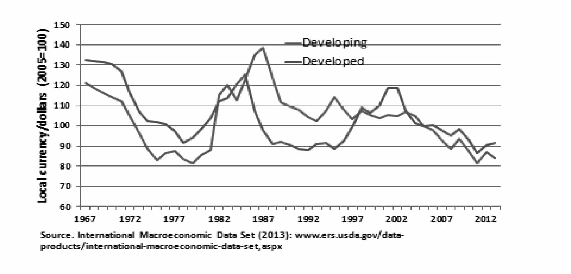
For turkey products, two measures of exchange rate volatility were considered, described as short-run and long-run, along with other factors to examine determinants of turkey trade flows. The empirical results showed that exchange rate volatility had a positive effect on turkey trade flows. In both the fixed effects and random effects models, short-and long-run exchange rate volatility coefficients were highly significant. The implications behind these results suggest that exchange rate volatility is not an impediment to turkey trade. In fact, exchange rate volatility in the short-run may expand turkey trade substantially. While intuitively one would expect exchange rate volatility to have a negative effect on turkey trade given the risk adverse attitudes of most producers, De Grauwe suggested that risk adverse producers and firms can benefit from exporting even when exchange rates are volatile. How is this possible? It is possible that some of the movements in exchange rates among countries are predictable which, in turn, reduce the level of risk associated with trade (Moledina et al., Reference MOLEDINA, ROE and SHANE2010). Figure 2 shows the long-term volatility of exchange rates for developing and developed countries. Exchange rates in developing countries have appreciated relative to the dollar for the last 25 years (from 1988 to 2012), while the exchange rates of developed countries have only appreciated over the last 10 years of that period (from 2003 to 2012). These patterns enable importing and exporting countries to anticipate changes in exchange rate volatility and respond appropriately to it.
The real exchange rate index for developing countries has had a long period of appreciation.
A reason why the exchange rate volatility effect is positive is because producers could benefit from instability if it is effectively managed and anticipated (Oi, Reference OI1961; Just et al., Reference JUST, HUETH and SCHMITZ1982). There are only a few large companies that export turkey. The size of these companies should warrant investment in resources to manage fluctuations in exchange rates to their advantage and hence export more. The market power of these exporters relative to importers could allow such behaviours without importers being able to adjust accordingly. Thus, exporters can benefit from countries with highly volatile currencies by offering high prices when exchange rates change in their favour and limit exports otherwise. This study revealed that the effect of exchange rate volatility on turkey trade is positive and highly significant in all models. Findings from this study agreed with Langley et al. (Reference LANGLEY, GIUGALE, MEYERS and HALLAHAN2000) as well as Awokuse and Yuan (Reference AWOKUSE and YUAN2006) who suggested that the measures of volatility make a difference.
In addition, the empirical results indicated that population has a positive effect on turkey trade flows. Real GDP also matters and had a positive impact on turkey trade for both importing and exporting countries. As expected, these findings show that as real GDP increases countries will trade more. Distance from the exporting country to the importing country has the appropriate sign, but was statistically significant only during the long-run, which suggests that distance plays a significant role in trade decision among countries. FTAs in particular, NAFTA and EU-27 have had positive impacts on turkey trade flows which maybe implications or incentives for newly established FTAs and their potential impacts on other agricultural products.