

1. INTRODUCTION
Education is relevant. The lack of complement is intentional as the sentence could have many different endings since education is an important determinant of most societal outcomes, from level of economic development [Lutz et al. (Reference Lutz, Cuaresma and Sanderson2008)] to innovation capacity [Pelkonen and Teräväinen-Litardo (Reference Pelkonen, Teräväinen-Litardo and Terro2013)], from demographic behavior [Lutz and Skirbekk (Reference Lutz, Skirbekk, Lutz, Butz and KC2014)] to adaptive capacity to environmental change [Lutz et al. (Reference Lutz, Muttarak and Striessnig2014b)], from conflict prevention [Østby and Urdal (Reference Østby and Urdal2011)] to women's autonomy [Jejeebhoy (Reference Jejeebhoy1995)], etc. To demonstrate the significance of education in – economic, environmental, technological, etc. – models, appropriate, and good quality data on present as well as on the past are crucial (Cohen and Soto, Reference Cohen and Soto2007). Indeed, patchy data and flaws in time series are rendering the use of education data in models problematic and impacting on their outcomes. Internationally comparable time series are, however, not readily at hand. This is surprising given that international bodies such as UNESCO – the United Nations Educational, Scientific and Cultural Organization – collect education data. Most data collections, however, take the data at face value and do not deal with inconsistencies. As a result, reliable data on education stocks – the educational attainment of adult population – are difficult to obtain although education data were collected for many years in censuses and surveys, but not consistently across time and countries.
Several research teams came up with the idea to reconstruct and harmonize time series on levels of education attainment – which stems from enrolment data that are more readily available than education stocks. Those reconstruction efforts can be divided into two main schools. The first approach which was primarily developed by Barro and Lee (Reference Barro and Lee1993, and additional versions in 2001, 2013, 2015) and further used by other researchers such as Cohen and Soto (Reference Cohen and Soto2007), and De la Fuente and Doménech (Reference De la Fuente and Doménech2000), to cite the most important ones, was to use the existing data points to inter/extrapolate the missing data points using several methods such as the perpetual inventory method (PIM). In 2007, Lutz et al. (Reference Lutz, Goujon, KC and Sanderson2007) proposed a second reconstruction approach based on multistate population projection methodology using the main characteristic of education, namely that it is acquired primarily at young ages and that it does not change later in life for most people. Hence, the education distribution of a population at any time t can be translated into the distribution at time t-n with some assumptions about how population evolved, i.e. the mortality and migration differentials and the education transitions. This approach, which does not depend so much on historical data points – except for the validation – was later adopted and adapted by Barro and Lee (Reference Barro and Lee2013), Cohen and Leker (Reference Cohen and Leker2014), and De la Fuente and Doménech, (Reference De la Fuente and Doménech2012).
To overcome the gaps in existing time series we have collected, harmonized, reconstructed, and validated large amount of data coming from multiple data sources. The outcome of this exercise is to this date the most comprehensive harmonized dataset on educational attainment. It covers 171 countries for the period 1970–2010, classified into six comparable educational levels and data are consistent across time, cohorts, and countries. The main difference between this version and that of Barro and Lee (Reference Barro and Lee2013) lies in the treatment of the historical data points. Most models require consistent time series on educational attainment in order not to pollute them with unnecessary jumps between subsequent periods/cohorts in the levels of educational attainment, a condition not necessarily met if one takes the historical data at face value [e.g. in Barro and Lee (Reference Barro and Lee2013)] as will be shown in the paper.
The dataset also has a prospective dimension as we project educational attainment into the future – to 2060 – using multistate population projections based on several scenarios for demographic and education change. The scenarios show the momentum of education development and provide an interesting window on the potential future of countries.
Because of the high level of consistency achieved by the dataset across countries and times, the findings are particularly robust, and can be used to show the importance of education for economic growth [see for instance, Crespo Cuaresma et al. (Reference Crespo, Wolfgang Lutz and Sanderson2014)]. In this paper, we present how the reconstructed data can be used to show descriptively different phenomena, related to the three most common gaps in education that are of geographical, gender, and generational order. While the gender gap has been declining across the last decades in most countries, women have still not caught up with men. Paradoxically, at the upper end of the education spectrum, the gender gap has been reversed with women having more education than men in many rich countries [Van Bavel (Reference Van Bavel2012)] but also in other settings. Concerning the geographical and generational aspect, the data also show that the diffusion of education within world regions or across cohorts follows the same patterns as other individual characteristics such as income or health with a convergence toward similar levels of educational attainment when overall levels of education are high. The momentum of education expansion is particularly visible in countries where investments in education were delayed and where many generations have been prevented from completing even primary education, not to mention higher levels.
The paper is organized as follows: After the introduction, the methodology used for the reconstruction of educational attainment time series is presented in the second section. This also includes some innovative techniques for calculating mean years of schooling (MYS), particularly accounting for incomplete levels of education. In the third section, we compare the results of the back projections with the other existing datasets as mentioned above. In the fourth section, we discuss some of the main results of the reconstruction along the lines of the three remaining gaps in education that exist in terms of gender, generation, and geography. In the last section, we offer a brief presentation of the methodology and the results of the projections to 2060 according to several scenarios, before concluding the paper with a discussion of the relevance of this reconstruction effort in the context of better understanding the major transition that took place during the 20th century in terms of education. Most importantly, the reconstructed and projected data are available online from the Wittgenstein Centre (WIC) Data Explorer: www.wittgensteincentre.org/dataexplorer/
2. METHODOLOGY
2.1. Back-Projection PrinciplesFootnote 1
The back projections that were used to reconstruct past levels of educational attainment rely on the principle that education is overwhelmingly acquired at young ages and is therefore a fixed attribute later in life. Hence, the educational attainment composition of a population encompasses the educational development of the past, which can be reconstructed along age groups. If we know the proportion of 50-year olds with post-secondary education in 2010 in country A, their share is a valid estimate of the proportion of 40-year olds in 2000 in the same country. This principle applies only to the population that is beyond schooling age i.e. we cannot reconstruct the population age 15–19 years in 1980 from the population aged 45–49 years in 2010. Hence, education transition matrices are required for the age groups where populations are likely to change their levels of education as explained below. Moreover, for the 35+ population, there are two phenomena that can upset the full equivalence through time: differential mortality and migration. For instance, if post-secondary educated people are less affected by mortality than lesser educated people – which has been demonstrated in the literature [Huisman et al. (Reference Huisman, Kunst, Bopp, Borgan, Borrell, Costa, Deboosere, Gadeyne, Glickman, Marinacci, Minder, Regidor, Valkonen and Mackenbach2005); Hummer and Lariscy (Reference Hummer, Lariscy, Rogers and Crimmins2011)] – then it is possible that the share of 40-year olds with post-secondary education will be less than the share of the 50-year old, their higher share at the age of 50 being the result of their lower mortality in the 10-year period. The mortality differentials are handled by means of education-specific life tables. Those differentials are more important at old ages when mortality rates are higher [Hummer and Hernandez (Reference Hummer and Hernandez2013)]. Another disturbance that can affect the back projections and has to be taken into account in the reconstruction is migration which rarely follows the education distribution of the host-country in terms of in-flows and out-flows. Lutz et al. (Reference Lutz, Goujon, KC and Sanderson2007) provide a summary of the back-projection methodology and of how migration and mortality differentials were dealt in the previous round of back projection. The same principles were used in the 2015 round of the WIC back projections with some amendments.
One amendment regards the maximum ages at which transitions are possible. In the earlier reconstruction [Lutz et al. (Reference Lutz, Goujon, KC and Sanderson2007)] with four levels of education (no education, primary, secondary, and post-secondary), the transition from no education to primary was possible until age 15–19 years, from primary to secondary until age 20–24 years, and from secondary to post-secondary until age 30–34 years. In the WIC (2015) dataset, findings from an earlier collection and harmonization effort [Bauer et al. (Reference Bauer, Potančoková, Goujon and KC2012)] were used, which revealed that quite frequently in the past, the age at transition to the next level of education showed considerable variation around the standard age at graduation, describing the theoretical age at which a person is supposed to graduate from a particular level of education. Hence, we leave the possibility for all transitions to happen until age 30–34 years, after which individuals are confined to their levels of education. This amendment leads to increased shares of population with tertiary education, taking into consideration the possibility of a transition at higher ages.
Based on these findings, we estimated country- and age-specific transition rates for education in the base-year to reflect the reality of educational transitions. However, due to the unavailability of consistent data, it was not possible to estimate the full transition matrix for all the periods in the past. Therefore, country-specific transition matrices were assumed to be constant over the back-projection period. This assumption could introduce a bias at both ends of the educational scale. Countries which had an elitist education system in the past might have had higher transition rates at earlier ages (compared to the standard graduation age) than now when the education has become more egalitarian and less advantaged pupils tend to transit to the next level later or spend more time to finish earlier educational levels. Reversely, in some countries where the average school entry occurred at older ages than the standard graduation age, improvements in the access to modern education may decrease the age at school entrance and increase the speed of attaining the next school level [Bauer et al. (Reference Bauer, Potančoková, Goujon and KC2012)]. However, the bias introduced by the constant transition matrices does not affect the ultimate levels of education that were checked against historical data during the extensive validation exercise (see Section 2.5).
The WIC (2015) back-projection methodology also differs from the earlier one [Lutz et al. (Reference Lutz, Goujon, KC and Sanderson2007)] in terms of the differential mortality by education. Both datasets rely on a standard schedule of mortality differentials. However, Lutz et al. (Reference Lutz, Goujon, KC and Sanderson2007) assumed that the mortality differential expressed in terms of life expectancy at age 15 years (e15) between the highest and the lowest education categories was 5 years for both sexes with a 1–2–2 year partition of the total difference between the no education, primary, secondary, and post-secondary education categories. In WIC (2015), the differentials were revised in two ways. First, since the education differentials were found to be larger among men than women [Lutz et al. (Reference Lutz, Butz and KC2014a)], the difference in e15 between the highest and the lowest education categories was set to 6 years for men and 4 years for women. Second, we assume the education differential in e15 to have a 1–1–2–1–1 year-pattern between the no education, some primary, completed primary, lower, upper, and post-secondary education levels, respectively – and the same proportionally for women [K.C. et al. (Reference K.C., Striessnig, Barakat and Speringer2015)].
At each step of the back projection, the United Nations (UN) estimates of life tables for the population [United Nations (2011)] are disaggregated into education specific life tables using the sex specific educational differentials in mortality as described in Lutz et al (Reference Lutz, Goujon, KC and Sanderson2007). The education, age, and sex specific survival ratios are applied to back project the population in 5-year steps. The total age–sex specific populations are then adjusted proportionally to match the UN age–sex distribution in the 1970–2005 period.
Finally, the education transition matrices are applied to back project the populations in the 15–34 years age groups. By virtue of going into the past, the whole process does not have to consider fertility.
The back projections go back until 1970 in this version mostly because we rely on base-year data around the year 2000–2010, meaning for instance that we reconstruct the education of 35–39 years old in 1970 using the education of 75–79 years old in 2010, which would become problematic if the population of reference is among the oldest old in the population of reference. For instance, in this example in 1960, to reconstruct the education of the 35–39 year olds, we would need the education level of the 85–89 years old in 2010. This age group in most countries is quite small and has been strongly affected by mortality differentials in education, distorting the education structure. The education distribution in the highest age group 100 years plus is assigned according to a logistic model fit derived from the base-year data [K.C. et al. (Reference K.C., Striessnig, Barakat and Speringer2015)]. In order, to reconstruct further in time using a similar methodology, one would need to complement the existing data with more historical one, an option that we are exploring at the moment in a project to estimate changes in education in the 20th Century.Footnote 2 Since the back projections rely mostly on data for the base year, it is highly important to arrive at a high quality base data, which is explained in the next section.
2.2. Harmonizing the Base Year Data
As mentioned in Section 2.1, the back- and forward-projections depend highly on the base-year dataset. However, no comprehensive datasets offer detailed and accurate data on educational attainment comparable across countries. Only UNESCO collects this information but with some flaws that will be mentioned in Section 3.2. The new base-year dataset of most recent information on population by level of educational attainment by age and sex was developed and documented in Bauer et al. (Reference Bauer, Potančoková, Goujon and KC2012). It served as the basis for the projections [Lutz et al. (Reference Lutz, Butz and KC2014a)] and the back projections. Compared with the earlier IIASA/VIDFootnote 3 harmonization exercise [Lutz et al. (Reference Lutz, Goujon, KC and Sanderson2007)], the number of educational categories was increased from four to six and the coverage was expanded from 120 to 171 countries.
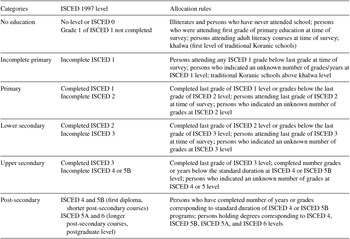
The dataset uses the information from national census data from several sources (IPUMS,Footnote 4 EUROSTAT, CELADE,Footnote 5 National Statistical Offices [NSO], etc.), as well as data from various surveys (Labor Force Surveys [LFS], Demographic and Health Surveys [DHS], Multiple Indicator Cluster Surveys [MICS], national surveys, etc.), for the period between 1998 and 2010. In a second step, a thorough harmonization procedure of national educational attainment, data was conducted based on the ISCEDFootnote 6 1997 classification [UNESCO (2006)]. Standardized procedures have been developed to differentiate between completed and incomplete level [Potancoková et al. (Reference Potancoková, K.C. and Goujon2014)], and to allocate country-specific educational categorizations into ISCED 1997. Table 1 summarizes the definitions of the six categories, their correspondence to ISCED 1997, and the main allocation rules.
Categories of educational attainment and allocation rules

Note: The post-secondary level encompasses non-tertiary and tertiary.
Detailed information about the data harmonization methodology can be found in Bauer et al. (Reference Bauer, Potančoková, Goujon and KC2012). Furthermore, those countries with data sources other than 2010 were projected to 2010 by applying the UN's estimates of fertility, mortality, and migration in order to provide the absolute population by age, sex, and education [K.C. et al. (Reference K.C., Striessnig, Barakat and Speringer2015)].
The resulting dataset represents the state of the world education according to ISCED 1997. It should be noted ISCED is, just like any other classification, a generalization and thus cannot reflect all the various details and particularities of the educational systems of every country, as well as the quality of education. However, the dataset is one of the most comprehensive collections of information on global human capital in terms of coverage, sample size, level of detail, and accuracy with respect to data harmonization. This allows for instance for the development of the transition model explained below, which is one of the particularities of the back and forward population projection methodology.
2.3. Transition Model
In reconstructing the educational attainment of, for example, 40-year-olds in 1990 from that of 50-year-olds in 2000, it is sufficient to consider mortality (and migration). An implicit assumption is that only few people gain higher formal education credentials in their 50s. This argument becomes weaker, however, the further back in time we proceed with the reconstruction. We can be much less confident that a university graduate aged 52 years in the year 2000 was already a university graduate at age 27 years in 1980, much less at age 22 years in 1975 (indeed, the likelihood that (s)he was certainly depends partly on the home country and the structure of its education system). In reconstructing distributions of attainment-by-age, it therefore becomes necessary to specify the age schedules at which individuals transition from one attainment status to the next.
Note that the reconstruction model that we have developed – presented in more details in Barakat and Durham (Reference Barakat, Durham, Wolfgang, Butz and KC2014) – ultimately requires not transition rates between attainment at time t and t+5, but the shares of different attainment levels at ages 15–19, 20–24, and 25–29 years, conditional on (presumed) final attainment at age 30–34 years or above. It means that we do not model the education dynamics (transition rates) but rather the educational distribution (shares by education) within the age groups 15–19 to 30–34 years. Estimating these conditional “backward” schedules directly, rather than deriving them from rates, allows for a more natural expression of time trends in attainment levels, is more parsimonious in a setting where there is no microsimulation of individuals, only of evolving aggregate shares, and arguably corresponds more closely to the framing of domain knowledge.
In an ideal situation, individual time series data for attainment by age would allow for the empirical estimation of these age schedules. Unfortunately, this is not possible in general with aggregate cross-sectional data, which are under-determined with respect to timing. It is therefore necessary to inject structural assumptions to constrain the estimation. A simple synthetic cohort perspective is not feasible, since the necessary assumption of stable levels of attainment over time is obviously false, and the cross-sectional patterns are not guaranteed to be logically consistent from a cohort perspective (i.e. they may involve supposed declines in highest attainment over age).
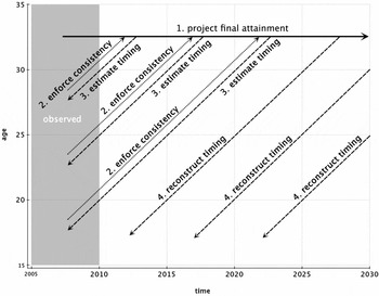
We overcome this difficulty by using a two-step analysis. In a first step, the raw transition schedules are estimated for each country based on short-term projections of the education of the 30–34 years age group. The projections are then compared with the attainment observed in the base year for the age groups 15–19, 20–24, and 25–29 years. For example, if 40% of the 30–34 year old are projected to have completed post-secondary education in the year 2015, and 30% are observed to do so in the 25–29 years age-group in 2010 – the base-year – then it means that ¼ of those who complete post-secondary education do so between the age of 25–29 and 30–34 years. This is repeated for the other age groups (15–19 and 20–24 years) with different projection horizon for the 30–34 years age group, and the same for all education categories (as schematized in Figure 1). In case the attainment at the observed younger age already exceeds the ultimate attainment projected for the cohort in question, the projection is adjusted upwards.
Short-term reconciliation between projected attainment at age 30–34 years and observed attainment at younger ages.

The schedules estimated in the first step are guaranteed to be logically consistent in a narrow sense, but are still numerically unstable, reflecting the difficulty of deriving timing from cross-sectional information in countries whose baseline population attainment at younger ages is highly irregular due to rapid educational change, declining attainment, or possibly migration. In a second step, an optimization technique is used to determine logically consistent schedules that minimize the distance between the country-specific first-stage schedules (with a weight of 0.7) and a standard set of schedules (with a weight of 0.3). These weights were picked by inspection as providing a sensible compromise between maintaining country differences, but removing artifacts that can occur in the raw empirical schedules in countries whose baseline population attainment at younger ages is highly irregular due to rapid educational change, declining attainment, or possibly migration. The standard set of schedules corresponds to a stylized 6+3+3+3 (years) system for primary, lower secondary, upper secondary, and post-secondary,Footnote 7 while taking into account the age-spread within 5-year age groups that delimit the age structure used in all models. For instance, in the 15–19 year age groups, some teenagers will have completed lower secondary education while others will have completed upper-secondary education. The transition timing as estimated and outlined above is then used both to project attainment at ages below 30 years from the projection of attainment at ages 30–34 years, as well as for the historical reconstruction.
2.4. Mean Years of Schooling
The indicator of MYS is frequently used for comparison across countries and time as it has the advantage of expressing the quantity of educational attainment present in a population in a single number. To compute MYS, one needs information on shares of persons with a given educational attainment level and duration of schooling for these levels. As straightforward as the computation of MYS may seem, it is at the same time complex for three main reasons. First, standard duration of schooling varies across countries and time as education systems evolve to respond to present-day needs. Second, the calculation is biased by the presence of pupils/students who do not complete the full course at any level, which amounts to substantial shares in some countries. Third, a large spectrum of courses at post-secondary level ranging from short 1–2 year certificate trainings to full post-secondary education completed by bachelor or master degree (or their equivalents) results in a necessity to make an assumption on the average number years of schooling to attribute to this education category.
Our calculations detailed in Potancoková et al. (Reference Potancoková, K.C. and Goujon2014) are based on disaggregated data by age (5-year age groups) and sex. We address the first point by relying on the information on standard duration of schooling compiled by the UNESCO Institute for Statistics (UIS) database.Footnote 8 However, this information is available only back to 1970, thus, for the cohorts who have entered education system prior to this date we assume the same durations as for the last reported year. As for the average duration for those with post-secondary education, 4 years of additional schooling after completion of upper-secondary (ISCED 3A) training seems to be the best estimate, in spite of country-specific variation.Footnote 9
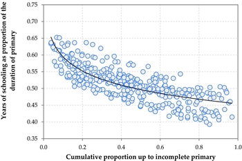
The main challenge lies in the estimate of the number of years spent in primary education for those who did not complete the full grade, which correspond to significant shares in developing countries as well as among the older cohorts in advanced countries. Other datasets e.g. Barro and Lee (Reference Barro and Lee2013) or De la Fuente and Doménech (Reference De la Fuente and Doménech2012), simplify by attributing half the duration of complete primary education to this group. Our hypothesis was that the number of completed years at primary level might be positively correlated with the overall level of education, meaning the higher the education level of the population is at the aggregate level, the higher the number of completed years in primary for those who do not complete. Moreover, we would expect variations not only by country but as well over time so that younger cohorts would complete more years within primary level compared to older ones. The analysis based on several datasets where both attainment levels and numbers of grades completed were providedFootnote 10 confirmed the hypothesis and showed that the higher the share of population with at most incomplete primary education, the earlier the average dropout occurred within the primary cycle as shown in Figure 2. The hypothesis holds across countries and cohorts although the number of years varies across different regions. Hence, we have developed a set of region-specific models – for Latin America, South-East Asia, South Asia, Sub-Saharan Africa, and Arab countries – of number of years at incomplete primary level to apply to the countries without detailed information on individual duration of schooling [see also Potancoková et al. (Reference Potancoková, K.C. and Goujon2014) for detailed information].
Relationship between duration of incomplete primary education (ISCED 1) and cumulative proportion of up to incomplete primary by cohorts aged 25–80+ years in Latin America.

Even small differences in durations of schooling and attainment shares result in different estimates of MYS for individual countries and across various datasets. A thorough harmonization of educational attainment categories and improved assumptions of standard durations of schooling result in better correspondence between the estimated MYS and those in observed values in microdata as shown by the description of the validation exercise in the next section.
2.5. Validation
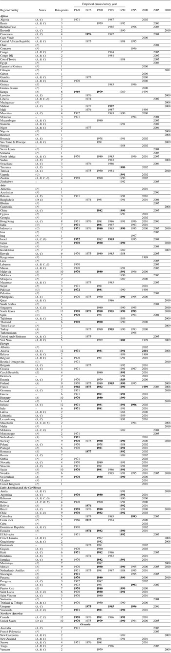
As mentioned in Sections 2.1 and 2.3, the back projections result from a model with assumptions related to differential mortality (including migration) and education transitions. We present in this section the validation methodology. The result of the validation is discussed in Section 3. We chose a modeling approach over interpolation between existing data points because of the flaws present in the data. While the historical data points do not enter the model, the outcome of the historical reconstruction of educational attainment is validated against other estimates of historical educational attainment as well as harmonized empirical datasets. We focused on data from censuses available from IPUMS [Ruggles et al. (Reference Ruggles, McCaa, Sobek and Cleveland2015)], NSOs which show better fitting accuracies to the WIC (2015) back-projection dataset, but also from UIS which are exhaustive in terms of countries. Other empirical data sources (for instance, survey data from DHS) were not used because of problems associated with education.
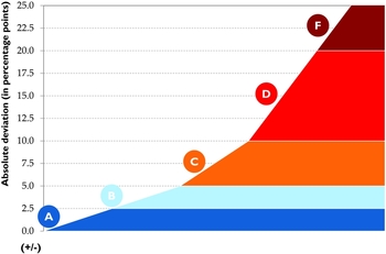
The comparison between WIC (2015) and available historical data points is performed on the proportional share of the six education categories in the population aged 25 years and over (see Table A.1 for a complete list of available historical data). We measure the absolute differences in percentage points (pp) between the corresponding educational categories. The education category with the highest deviation between data points determines the validation categorization. The deviations in pp are categorized into five groups by predefined thresholds (see Figure 3). The labels of those five groups are referring to the American school grading scheme (A, B, C, D, and F). Therefore, deviations beneath 5 pp are labeled as good (A) or rather good (B). We made this distinction to highlight the countries with very high accuracy of fit (beneath 2.5 pp). Higher deviations above 5 pp are divided into the categories rather bad (C) or bad (D) to get a more differentiated picture of the level of deviations between empirical and model data. Countries and data series with a deviation above 20 pp and no chance of improving the matching accuracy are allocated to the category not usable (F), since the deviation beyond that point cannot be explained whereas most of the deviations below the 20 pp threshold can be explained [Speringer et al. (Reference Speringer, Goujon, Eder, KC, Bauer and Potančoková2015)].
Validation categorization scheme by (+/−) absolute deviation (in percentage points).

The validation is a two-step procedure in that we first compare the harmonized empirical data with the WIC (2015) dataset and attribute a validation category, depending on the country- and education-specific deviation in a certain data point, before we search in a second step for possible sources for the deviation. One source of deviation could be issues occurring with the harmonization of educational categories from historical datasets, like mistakes in the recoding of educational categories due to missing or overlapping categories in the source data. Another issue could occur from the reliability of the source data that would require the reviewing of data documentation and related literature to identify flaws in the census quality, or deviations due to education specific migration movements. One way to identify such flaws in the historical time series is to apply an “age-cohort analysis” (ACA) that checks for heaps in the development of a specific birth cohort along different points in time, e.g. the 40–45 years age group in 1980 and the 50–55 years age group in 1990 [Speringer et al. (Reference Speringer, Goujon, Eder, KC, Bauer and Potančoková2015)].
3. COMPARISONS WITH OTHER DATASETS
We will compare the WIC (2015) reconstruction to two types of dataset on educational attainment: empirical and reconstructed. For the first type, we focus on three main data sources, IPUMS, NSO, and UIS. For the latter, after mentioning the most important efforts, we concentrate the comparison on the most widely used and referenced ones, the [Barro and Lee dataset (Reference Barro and Lee2013)] and [de la Fuente and Doménech (Reference De la Fuente and Doménech2012)]. We also shortly highlight the differences existing between the WIC (2015) dataset and the earlier version published in [Lutz et al. (Reference Lutz, Goujon, KC and Sanderson2007)].
3.1. Comparison with Empirical Datasets
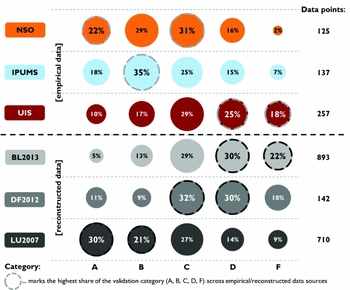
The WIC (2015) dataset was validated and compared against some empirical datasets namely IPUMS, NSOs, and UIS (see Figure 4). The IPUMS dataset [Ruggles et al. (Reference Ruggles, McCaa, Sobek and Cleveland2015)] allows for the validation of 55 countries or 137 census data points with educational attainment, and shows relatively high matching with the WIC (2015) dataset: About 73 datasets show an accuracy of category A or B, which means an absolute difference between WIC (2015) and the harmonized IPUMS data beneath 5 pp.
Validation result by data sources and proportion data points by validation category. Notes: BL2013 – [Barro and Lee (Reference Barro and Lee2013)] | DF2012 – [De la Fuente and Doménech (Reference De la Fuente and Doménech2012)] | LUReference Lutz, Goujon, KC and Sanderson2007 – [Lutz et al. (Reference Lutz, Goujon, KC and Sanderson2007)].

However, the matching is better in the 1990 census year with 37 datasets out of which 24 are categorized as A or B, less so as we move back in time. This loss of matching may be due to categorization problem in IPUMS as it was shown for France [Speringer et al. (Reference Speringer, Goujon, Eder, KC, Bauer and Potančoková2015)]. Another issue that can occur in the IPUMS dataset is that educational levels are aggregated in a way that do not allow for comparison with WIC (2015) educational categories, e.g. the Netherlands (1971) or the United Kingdom (1991, 2001).
With NSO data, we were able to validate 54 countries and 125 data points out of which almost half exhibit a good or rather good matching with the WIC (2015) back-projection dataset. Issues that lead to a deviation of the WIC (2015) dataset from the NSO data are the same as observed with IPUMS. For some countries, the comparison was simply impossible to make e.g. Canada (1971), Switzerland (1971), and Latvia (1989), due to problems with data reliability and categorization. It is worth noting that we accounted for changes in national education systems when harmonizing historical education dataset e.g. in the case of Spain, so this issue was taken care of by construct. In other cases, it seems that the WIC (2015) back-projection model sometimes over- or under-estimates the pace of the transition between educational categories e.g. in the case of Hungary. The reason lies mostly in the transition model, which utilizes both standard schedules, and country related information for the recent past, not taking into account the more distant trends of the past (see Section 2.3).
The third empirical dataset that was used for the comparison was that of the UIS which offers 257 data points on educational attainment for 127 countries. However, the UIS data exhibits the lowest matching accuracy with the WIC (2015) dataset: Only 70 datasets (27%) with a good or rather good matching accuracy. In 47 cases, the difference is above 20 pp equivalent to category F mostly due to the inconsistent coding of the education categories, especially regarding the classification of complete and incomplete education, and the aggregation or overlapping of categories.
It is understandable that the WIC (2015) dataset matches better with NSO and IPUMS datasets since those are often detailed in terms of education categories and hence allow for a close fit by allocation. The UIS dataset on the other hand is constructed with fixed large categories – filled by NSO but with no control other the distribution – is more likely to diverge from the WIC (2015) as shown in Figure 4.
3.2. Comparison with Other Reconstruction Exercises
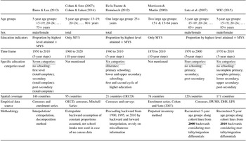
There exists only a few datasets that try to reconstruct the education structure for various populations in the past. Their characteristics are presented in Table A.3. They diverge in three main ways from the present work: methodology, data used, and scope, although their features have changed over time. They all have in common, including the WIC (2015) dataset that they have to rely on an already existing data collection on education by age and sex (see section 2.2).
In terms of methodology, some authors [Barro and Lee (Reference Barro and Lee1993, Reference Barro and Lee2001, Reference Barro and Lee2013); Morrisson and Murtin (Reference Morrisson and Murtin2009)] have been at first using the PIM in order to fill the gap of missing data on educational attainment by translating enrolment data into educational attainment. While the idea is valid, enrolment data suffer from even more flaws than attainment – especially in countries with poor statistical systems, e.g. in Africa [Chapman and Boothroyd (Reference Chapman and Boothroyd1988); Jansen (Reference Jansen2005); Samoff (Reference Samoff1991)]. Furthermore, in many developing countries, local governments tend to over-report enrolment numbers to gain a better financial support from their government or international donors. And lastly, the translation of enrolment into level of education, whether it was completed or not, requires even more assumptions. The methodology used for the reconstruction in Lutz et al. (Reference Lutz, Goujon, KC and Sanderson2007) and the WIC (2015) dataset relies mostly on the base year data. In their latest revision, Barro and Lee (Reference Barro and Lee2013) adopt a methodology resembling our approach of using the stability of education along cohort lines, and assuming differential mortality by education for the population – in their case aged 65 years plus, while we consider the mortality differentials starting from the age of 15 years. Thereby, the authors estimated survival ratios by distinguishing between two broad educational groups, a less-educated population (uneducated and people who have reached the primary level) and a more-educated population (reached at least secondary schooling), as well as for broad groups of OECD and non-OECD countries. Based on their collected data points, Barro and Lee (Reference Barro and Lee2013) interpolate/extrapolate the population by age and education between/from empirical data points forward and backward. De la Fuente and Doménech (Reference De la Fuente and Doménech2000; Reference De la Fuente and Doménech2012) also adapt the methods from Cohen and Soto (Reference Cohen and Soto2007) and Barro and Lee (Reference Barro and Lee2013) to interpolate/extrapolate backward and forward by adding miscellaneous information and their professional judgment to create smooth time series of educational attainment. The advantage of this method is its feasibility as it relies on existing historical data. However, it depends on the accuracy of historical dataset which if lacking can hamper the quality of the reconstructed dataset as shown below.
One of the main differences between all datasets lies in the original data that are used to either back project, interpolate, or extrapolate. In their first estimates, Barro and Lee (Reference Barro and Lee1993, Reference Barro and Lee2001, and Reference Barro and Lee2013) used predominantly UNESCO data which are barely harmonized (as described in Section 3.1). The latest version [Barro and Lee (Reference Barro and Lee2013)] is using more census data from national statistics offices, as it has turned out to be the most reliable data source. Nevertheless, the issue of not harmonized input data are still visible in their calculations which results in unusual jumps in the time series or in same shares of educational attainment for different 5-year age groups, when aggregated input data are used [Speringer et al. (Reference Speringer, Goujon, Eder, KC, Bauer and Potančoková2015)].
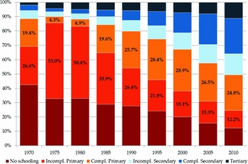
This is illustrated in Figure 5 for the case of Brazil where the Barro and Lee dataset shows a doubling of incomplete primary education from 1970 to 1975 and in the same period, a decrease of complete primary education from 19% to 4%. From 1980 to 1985, the share of people aged 25 years plus with completed primary education suddenly quadruples again to almost 20%. A consideration of data from the NSO or IPUMS would have prevented this discrepancy to occur. The case of Brazil is not an isolated one but rather an indication of a more general problem in the Barro and Lee estimates which relies heavily on their confidence in the accuracy of their original dataset. This becomes especially an issue for countries for which the reconstruction is based on just one or two data points, which is the case for 79 countries out of 146. Similar issues were found in De la Fuente and Doménech dataset (Reference De la Fuente and Doménech2012), where there are some problems with the processing and harmonization of the available educational data as basis for filling the data gaps. Another issue has to do with the method to decompose incomplete and completed levels [see Bauer et al. (Reference Bauer, Potančoková, Goujon and KC2012); Potančoková et al. (Reference Potancoková, K.C. and Goujon2014)] that causes several oddities in the time series, e.g. for Belize, Bolivia, Mozambique, Senegal, South Africa, Swaziland. In the WIC (2015), we have tried to circumvent the data quality and consistency issue by applying some procedures: (1) an extensive data collection, (2) a careful selection of the best data sources, (3) the harmonization of the data, and (4) a high level of detail considering age, sex, and education categories, as explained in Section 2.2 and more extensively in Bauer et al. (Reference Bauer, Potančoková, Goujon and KC2012).
Total population aged 25 years plus by education, Brazil, 1970–2010 [Barro and Lee (Reference Barro and Lee2013)].

The final difference lies also in the type of output and the scope. First, some provide only data on MYS instead of educational attainment [Cohen and Soto (Reference Cohen and Soto2007); Cohen and Leker (Reference Cohen and Leker2014); Morrisson and Murtin (Reference Morrisson and Murtin2009)]. Second, they lack basic demographic indicators like sex and detailed age groups [Cohen and Soto (Reference Cohen and Soto2007); Cohen and Leker (Reference Cohen and Leker2014); de la Fuente and Doménech (Reference De la Fuente and Doménech2012); Morrisson and Murtin (Reference Morrisson and Murtin2009)], whereas it has been shown [Lutz et al. (Reference Lutz, Cuaresma and Sanderson2008)] that the consideration of these two parameters helps to explain differences in economic outcome in many countries.
Barro and Lee (Reference Barro and Lee2013) still is more comprehensive in terms of time span compared to WIC (2015) as it provides many education indicators by age and sex and over a long time period from 1950 to 2010, whereas the WIC (2015) dataset only goes back to 1970. Since the WIC (2015) reconstruction uses the information contained in the age, sex, and education structure of the population around the year 2010, it would be difficult to reconstruct further in time and would require more historical data points, as explained in Section 2.1. On the other hand, the Barro and Lee (Reference Barro and Lee2013) dataset contains less countries (146 vs. 171) while they include 12 countriesFootnote 11 that are not listed in the WIC (2015) dataset. We excluded these countries mainly for the reason that those datasets are either hardly available from NSOs, the countries have a population beneath 100,000 or the data are of limited reliability.
These, among other factors, cause the discrepancies between the WIC (2015) and other data sets. For the Barro and Lee (Reference Barro and Lee2013) dataset, out of the 134 countries and 893 data points available for comparison, only 162 data points or 18% show an absolute difference of less than 5 pp (categories A [47] and B [115]). As shown in Figure 4, the vast majority of the 468 comparable data points deviates by more than 10 pp in one or more educational categories (categories D [270] and F [198]). The same difference is visible with the De la Fuente and Doménech (Reference De la Fuente and Doménech2012) dataset which hardly matches because 68 of the 142 data points fall in the category D or F (see Figure 4).
The main differences between the 2007 Lutz et al. dataset and the WIC (2015) dataset lie in the methodology (see Section 2.1). Lutz et al. also used 2000 as the base year, and had only four educational categories, namely no schooling, primary, secondary, and tertiary education. The tertiary education in Lutz et al. (Reference Lutz, Goujon, KC and Sanderson2007) is not one to one comparable to the post-secondary education category in the WIC (2015) dataset which includes the ISCED 4 category (post-secondary non-tertiary) which was under secondary in the previous dataset. For some countries, it does not affect the distribution, for others it does, e.g. Singapore. When comparing the 710 data points for 119 countriesFootnote 12 from 1970 onwards for the two datasets, we find that about 210 (30%) are fitting good and 147 (21%) rather good (see Figure 4). The source for deviations in all other cases originates mainly from the different base-year data, data sources, and education classification between the two datasets. Some other differences result from the allocation between completed primary and completed lower secondary, which in many cases represents basic or compulsory education. In Lutz et al. (Reference Lutz, Goujon, KC and Sanderson2007), when the data could not be disaggregated between the two categories, it was allocated as a rule to the lower education category primary education. Altogether, we observe a significant difference between the two datasets in the case of 12 countries.Footnote 13
The comparison between the WIC (2015) datasets and others point at the general difficulty of reconstructing time series based on partial and inconsistent data. This has implications for users of time series on education. The WIC (2015) has the advantage that it has been thoroughly checked for consistency and hence is likelier to be more reliable and hence more robust as input in all kinds of regression models.
4. RESULTS
Having information on the levels of educational attainment in 5-year age groups, separately for men and women, for 171 countries allows for analyzing the diffusion of education within the 1970–2010 time frame period, and most particularly how inequalities have evolved. In this section, we will be focusing on the descriptive analysis of the three most common gaps in education that are of geographical, gender, and generational order. More analysis could be done – and it is our hope that more researchers will use the WIC (2015) dataset and its updates for their work – based on the back projections. Some research has already been implemented for instance to look at the relative impact of education and demography in what is called the demographic dividend [Crespo Cuaresma et al. (Reference Crespo, Wolfgang Lutz and Sanderson2014)].
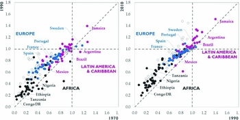
While the gender gap has been declining across the last decades in most countries, women have not caught up fully with men. They are still nowadays most numerous among the population who have not been at school at all – 63%, and this share is rather stable over time. It was 60% in 1970. Also unwavering is the absolute population of women aged 15 years and over (15+ years) without education, which has been around 500 million between 1970 and 2015. However and since the world population has been growing, the proportion of women without schooling has been declining from two-fifth of the population 15+ (44%) to one-fifth (18%). At the upper end of the education spectrum, Figure 6 shows the female to male ratio of population aged 25 years and over with upper-secondary and post-secondary education by country to illustrate differences between two points in time, between 1970 and 1990, and between 1990 and 2010. The dashed vertical and horizontal lines at value 1 indicate gender equilibrium in the respective year. The dashed diagonal line shows the difference between the points in time, e.g. every dot above the diagonal line shows an improvement between the two points in time.
Female to male ratio of population aged 25 years and over with upper secondary and higher education by country, colored by region, 1970 to 1990 and 1990 to 2010.

The vast majority of countries showed improvements in the gender balance in both time periods (1970 to 1990 and 1990 to 2010). It is particularly obvious for Europe and Latin America and Caribbean, less so in Africa which is slowly catching up but where many countries are still left behind. Noticeable are a few countries in Latin America and Caribbean, where the gender gap has been reversed with women having more education than men. In some settings, particularly in small population countries, this can be caused by strongly gendered international migration flows like in Jamaica [Thomas-Hope (Reference Thomas-Hope2002)] or Lesotho [Sparreboom and Sparreboom-Burger (Reference Sparreboom and Sparreboom-Burger1996)] where more educated men tend to migrate in higher proportion than more educated women. However, this worsening of the conditions for men has been shown in different settings, particularly at the level of higher education, and already from the 1980s onwards in many OECD (Organization for Economic Co-operation and Development) countries. An explanation could be that discouraged male students withdraw from education to enter the job market due to disillusionment regarding employment perspectives and the monetary returns to higher education. Also as shown by Fortin et al. in the United States (Reference Fortin, Oreopoulos and Phipps2015), men tend to have career plans for occupations early on in their school life, which often do not require advanced degrees. The situation is different for women who are more in need of a post-secondary education if they want to have a career – in opposition to a job. Despite the educational gains achieved by women, they continue to lag behind men in labor and economic outcome [Chamie (Reference Chamie2014)]. [DiPrete and Buchman (Reference DiPrete and Buchman2013)] showed that the reversal is complex with high levels of heterogeneity within genders and changing opportunities for women and men to utilize their skills.
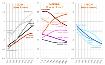
The variety of experiences in terms of the diffusion of education can also be seen in terms of the geographical gap. Not only have the several world regions evolved differently in an aggregate manner, but our research shows that there is a relationship as well between the overall level of education within a region and the difference between the countries within regions (Figure 7). This is an interesting feature which confirms that the diffusion of education follows the same patterns as other individual characteristics such as income or health [Wils and Goujon (Reference Wils and Goujon1998)]. It seems to show that at lower regional levels of education, countries within the regions are quite homogenous – mostly having similar MYS compared to the regional average, and the same at high levels of education but the diffusion pattern is interesting as countries are not progressing at the same speed from low level to high level and hence the gap between countries within a region is sometime quite important. This is best shown by looking at the patterns of regional development in terms of standard deviation of countries to the regional average for MYS in the 1970–2010 period as shown in Figure 7. At low levels of educational development – measured according to the criteria below 7 years of MYS in 2010 – the standard deviation is presently increasing between countries, which is the result of different speeds of educational development toward increasing educational attainment. This cluster (1) includes all sub-regions in Africa except southern Africa which belongs to the intermediate stage in the typology (cluster 2) with mixed patterns of deviation increasing or decreasing over the period of observation. Most Asian and Latin American sub-regions belong as well to this cluster (2). At higher education levels – categorized as MYS above 10 years in 2010 (cluster 3) – the deviation starts declining everywhere as shown for Europe, where the countries have converged toward similar levels of educational attainment and the difference between countries within regions are strongly declining.
Standard average deviation in MYS from regional average for population aged 25 to 59 years grouped by MYS 2010, 1970–2010.

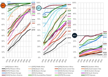
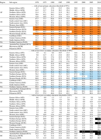
The different pace of education diffusion can be also measured by the time when countries and regions hit certain educational benchmarks. We selected three of them that are based on the existing literature. We measured them in the age group 30–34 years when most education transitions are completed. Universal primary education was formulated as 95% or higher with primary education – taking into consideration that 100% is rarely achieved due to migration of less educated population [see also Bruns et al. (Reference Bruns, Mingat and Rakotomalala2003); UNESCO (2015)]. For the second benchmark in terms of universal lower secondary education, which is more and more considered as the compulsory level of education, we assumed that it should encompass 90% of the population based on the European Union strategy recommendations [European Commission (2010); Roth and Thum (Reference Roth and Thum2010)]. The same sources provide the third benchmark in terms of the proportion with a post-secondary education which is assumed to be around 40%.
Figure 8 shows if and when different sub-regions surpassed the defined thresholds over time (see also Table A.2). There are eight sub-regions that have achieved universal primary: namely Eastern Asia, Eastern Europe, Northern Europe, Southern Europe, Western Europe, Northern America, Australia/New Zealand, and Polynesia, whereby Eastern Asia, Southern Europe, and Polynesia surpassed the threshold already in the 1980s and 1990s. In terms of “universal lower secondary” again the European regions, Northern America and Australia/New Zealand are the major world achievers with Eastern Europe and Northern America already surpassing the benchmark in the 1970s and the latest regions were Northern and Southern Europe in the 2000s. The reason for this fast increase in lower secondary and higher education, especially in Northern Europe, can be found in the huge financial investments in the countries of this region into education in the second half of the 20th Century. Noticeably, Eastern Asia had almost reached the benchmark in 2010.
Share of population aged 30 to 34 years with at least primary education (left), at least lower secondary (middle), and at least post-secondary education (right) by sub-region, 1970–2010.

Lastly, for the 40% benchmark with post-secondary education only a handful of regions exceeded the 40% threshold recently, namely Northern America, Australia/New Zealand, Northern and Western Europe. Noticeable is a slight drop in Northern America – but also in the other high educated regions – in the share with post-secondary education in the age cohort 30 to 34 years in the late 1980s and 1990s, which can most likely be explained by the inflow of lower educated migrants, the lesser need for post-secondary education in an economically flourishing era where for instance the United States had a still strong industrial sector that did not require higher education degrees but still offered relative high income. Not shown on Figure 8, a closer look shows that the drop occurs mostly among the male population, while women with post-secondary are overtaking the men in this period. Other regions are far from the 40% benchmark with a share between 10% and 20% (see Figure 8). The pace of change also shows that the increase in education is mostly occurring at primary and secondary levels.
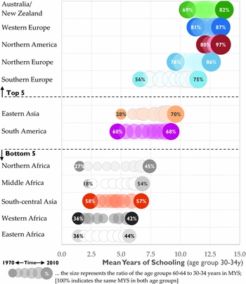
Another feature of societies where levels of educational attainment are increasing is that it is reflected in the difference in education between those who have been in school some time ago, e.g. the elderly and those who have left school just a few years ago. The difference in the composition of age structures plays an important in intergenerational accounting as shown for instance by D'albis and Moosa (Reference D'Albis and Moosa2015). In this section, we will look at the generational gap comparing principally the population aged 30–34 years and those aged 60–64 years, judging from the MYS for both age groups. On Figure 9, the MYS of the age group 30 to 34 years is represented on the x-axis and some selected regions on the y-axis (sorted by the level of MYS in 2010). There is one bubble for each year in 5-year steps from 1970 to 2010. The size of the bubble represents the ratio of MYS for age group 60–64 years to that for age group 30–34 years, i.e. 100% indicates the same number of MYS in both age groups.
MYS in the age group 30 to 34 years and the ratio of the age groups 60–64 to 30–34 years in MYS by selected regions, 1970–2010.

The results show not surprisingly the same sub-regions at the top as aforementioned, meaning with the highest level of MYS and the lowest level of intergenerational gap. While the Australia/New Zealand sub-region is the top country in terms of MYS of the 30–34 years age group, the gap is still substantial (82%) compared to North America (97%) and Western Europe (87%) where the improvements in schooling occurred some time ago and have already benefitted most people in the education system that are now growing old. Eastern Asia and South America provide some interesting aspects as both regions have similar levels of MYS throughout the period but the generational gap was much stronger in 1970 in Eastern Asia than it was in South America, still reaching the same levels in 2010. This is pointing at rapid increases in the former sub-region – education progress has been one of the key components in the success of the east Asian Tigers economies [Goujon and K.C. (Reference Goujon and K.C.2008)] – compared to less change across cohorts in the latter. Figure 9 shows that the sub-regions that have low levels of MYS do not have the same experience in terms of generational gap. While South-Central Asia, and to a lesser extent Eastern and Western Africa show very little difference in the evolution of the generational gap between 1970 and 2010, the changes were more abrupt in Northern Africa and Middle Africa. As was shown in Section 3, while other datasets could in principle allow for this type of analysis, none are as complete or include the level of details existing in WIC (2015), and moreover they do not offer the same degree of consistency between countries and across time.
5. PROJECTIONSFootnote 14
Besides reconstructing the past, the population of all 171 countries by education was projected into the future following the methodology of multistate population projections developed by Rogers (Reference Rogers1980). While the projections were carried out with a long-term perspective until 2100, we only consider educational attainment up to 2060 because the scenarios regarding future levels of education are implemented until then, and kept constant thereafter and we expect the meaning of levels of education to evolve beyond what we can imagine nowadays.
The projections are used to see how the world would look like in terms of size (by age and sex) and composition (by education) according to some scenarios about demographic and education developments, the latter being a novelty compared to most global population projections. The projections that were developed by a large team of researchers at the WIC for Demography and Global Human Capital are extensively documented in Lutz et al. (Reference Lutz, Butz and KC2014a) and in K.C. and Lutz (Reference K.C. and Lutz2014). The projection assumptions are developed using both models and expert opinions about the future direction of fertility, mortality, and migration. The experts notably assessed through an online questionnaire the validity of alternative arguments that impact on the major demographic trends. The demographic scenarios are also combined with hypothesis on future educational development. More details about the assumption making for the projections can be found in several chapters in Lutz et al. (Reference Lutz, Butz and KC2014a).Footnote 15 The scenarios that were developed are also interesting in the sense that the storylines were primary developed for the Fifth Assessment Report of the International Panel on Climate Change, an exercise that involved many experts outside of the realm of demography.
In developing the assumptions, we had to overcome several difficulties. First of all, there exists no international empirical time series on education-specific fertility, mortality, and migration trends over the recent or even more distant past. Plus, the expert knowledge on education-specific trends is very limited. Hence, the process of defining assumptions initially focused on defining the numerical values for overall fertility, mortality, and migration levels, not distinguishing by levels of educational attainment. In a second step, education-specific fertility and mortality assumptions over time were derived by assuming certain relative differentials between the vital rates of the different education groups and by assuming that the base scenario, the medium Global Education Trend (GET) scenario describes the future educational attainment trend that underlies the assumed aggregate level trends in vital rates.
5.1. Fertility Assumptions
Because the drivers of future fertility are very different between countries that are still in the process of fertility transition and those that are already toward the end of this global transition, the countries were divided in two sets: low-fertility and high-fertility countries based on period Total Fertility Rates (TFRs – a synthetic measure of the average number of children a woman would bear during her lifetime) for the period 2005–10 according to the United Nations (2011) – together with the countries levels of socio-economic development as assessed by the Human Development Index [UNDP (2011)]. The procedures chosen to derive the fertility trajectories differed somewhat between the high- and low-fertility groups. For the high-fertility group of countries, the assumption-making process consists of a four-stage approach.
-
1. We estimate a model of historical analogy (for all countries) by employing past levels and decreases of fertility across countries taken from the historical time-series estimated by the United Nations (2011). This methodology is quite similar to what the UNs assumed until 2010. We compared each country's level and decrease of fertility in the past 5-year interval to all countries that have undergone similar levels and decreases of fertility (+/− 10%) at any 5-year period between 1970 and 2005. Only countries that were exposed to comparable decreases in fertility (+/− 5 pp) relative to the previous period were considered in the calculation of the expected fertility decline. The mean fertility decline for all countries that is fulfilling these two constraints, represent the expected fertility decline for the following 5-year period.
-
2. We estimate the expected decrease of fertility by source experts from the 140 responses (for 37 countries) to the high-fertility module in the expert questionnaire by developing a model that translates responses from arguments to respective changes in fertility.
-
3. During the meeting with meta-experts in Nepal, we gained further insights into the most important drivers of fertility across world regions, and formulated numerical estimates of fertility (for 14 countries) in 2030 and 2050. From there, we calculated two rates of decrease, one from 2010 to 2030 and another from 2030 to 2050.
-
4. In a final step, we combined all three models by weighting the estimated fertility decreases of each respective model. Model results, meta-expert assumptions and source expert score-based values were weighted in the ratio 1:1:0.2. For countries that by this procedure reached a TFR of 1.6 children or lower in any period before 2100, the procedure chosen by the low-fertility group was enacted, implying a slow convergence toward a TFR of 1.75 children.
For the low-fertility countries, point estimates of the period TFR in 2030 and 2050 (medium scenario) were derived in several steps. Following the source experts’ judgments gathered in the online survey and the agreements reached during the discussions of the meta-expert meeting in Vienna, TFR scenarios for a number the key countries were derived. Based on these, the point estimates for all remaining low-fertility countries were derived by analogy. A special effort was made to account for the effect of the on-going economic recession in the near term by combining most recent information about annual fertility trends with the assumption that fertility rates were likely to fall somewhat in the most affected countries and that no country would see a fertility increase in the period 2010–15. As mentioned above for countries in the high-fertility group, it was assumed that period TFR levels in low-fertility countries would slowly converge to an average value of 1.75 children (with the convergence point in the year 2200).
The TFR were then translated into age-specific fertility rates (ASFR – the number of live births per 1,000 women in specific age groups) applying the period-specific age schedules of the UN-medium variant [for a detailed description of their methodology, see United Nations (2006)]. Country-specific differentials in fertility by level of education for the base year were obtained from the literature and from census and survey data [see also K.C. and Potančoková (Reference K.C. and Potančoková2013)]. Over time, the education differentials are assumed to converge to ratios of TFRs of 1.42, 1.42, 1.42, 1.35, 1.14, and one children, for the different education levels relative to post-secondary education. These values are assumed to be reached by the time TFR reaches 1.8 children per woman. For countries where the maximum differential is below 1.42 children in the base year, the relative ratios are kept constant at those lower levels.
5.2. Mortality Assumptions
As with fertility, the mortality assumptions are based on a combination of a statistical model and source and meta-expert assessments. The model itself is based on the general assumption of convergence which was one of the main outcomes of the meta-expert meeting in Costa Rica. The idea of a global mortality convergence is widely acknowledged [Wilson (Reference Wilson2001)]; however, there have been relatively few attempts to deal with convergence explicitly, e.g. Heuveline (Reference Heuveline1999). We specifically used the concept of sigma-convergence – meaning a reduction in the dispersion of levels of life expectancies across countries [Anand and Ravallion (Reference Anand and Ravallion1993); Bidani and Ravallion (Reference Bidani and Ravallion1997)] – in absolute terms in our model to produce female life expectancy forecasts for all countries covered by this study.
This convergence procedure was implemented in five steps:
-
1. First, Japan was identified as the current global forerunner in female life expectancy. Under the medium scenario, the life expectancy at birth of Japanese females is assumed to grow by 2 years per decade from 86.1 years in 2005–2010 to 104.2 in 2095–2100. Regional forerunners (22 regions) were identified, wherein female life expectancies were projected so that the change in life expectancies converges to the assumed change in Japan, that is, by 2 years per decade. This was implemented by applying a dynamic panel data model, autoregressive of order 1 with fixed effects, which was estimated with 2-step generalized method of moments (GMM) over the period 1980–2005.
-
2. Once the life expectancies for regional forerunners were projected, a similar model was applied for countries within each region that were assumed to follow their regional forerunners. This convergence model has the advantage that it is based on empirical data. In addition, it takes into account the heterogeneous country-specific historical experiences as well as differences in gains between forerunners and laggards over time and across regions.
-
3. In the third step, for HIV-affected countries and two high mortality countries (Haiti and Afghanistan), the UN Medium-Variant life expectancies (2011) were assumed until the period 2045–2050. After 2050 life expectancies to the end of the century were projected using the model with Namibia (as the forerunner country for this group of countries.)
-
4. In the fourth step, the model results were blended with the country-specific expert assessments until 2045–2050 by a weighting procedure: The result of the statistical model was assigned the weight of 1.0, the average of the meta-experts the weight 1.0 and the specification of each individual source expert who made a statement on a given country the weight 0.2.
-
5. In the final step, the result from step 4 in terms of net gains for the period 2010–2050 were used to re-estimate and modify the net-gains for the 2050–2100 period.
Similar steps were repeated for the high- and low-mortality scenarios. Once life expectancies at birth for 5-year periods during 2010–2100 were modeled for females in 196 countries, life expectancies for males were derived by applying the difference between the female and overall life expectancy in the UN medium variant [United Nations (2011)]. For a given sex-specific e0, life-tables were derived by interpolating and extrapolating (when the values were higher than the highest in the UN Medium variant) using country-specific life tables used in the UN-medium variant.
We introduce gender-specific education differentials in mortality as differences in life expectancy at age 15 years following the literature: The difference in life expectancy at age 15 years between the “no education” category and the post-secondary educated population is assumed to be of 6 years for men and 4 years for women. Between these extreme points, among males, we assume 2 years difference between “completed primary” and “completed lower secondary”, and 1 year for the remaining levels of attainment. Likewise, for females, we proportionally adjust to the lower assumption of a 4 years differential overall. Finally, for children up to age 15 years, the differential mortality is introduced through the mother's education. We assume that the differentials in terms of relative ratio of mortality rates with respect to the completed upper-secondary category are 1.8, 1.7, 1.6, 1.4, 1.0, and 0.8, in ascending order of educational attainment. These values are based on the averages of under-five mortality rates in the DHS countries.
5.3. Migration Assumptions
The migration component of the projections represents a significant innovation in the way migration is handled in global population projections. Instead of the conventional approach of net-migration models, we made use of bilateral migration flow estimates by Abel and Sander (Reference Abel and Sander2014). These estimates of country-to-country migration flows for 5-year periods allow us to use a bi-regional cohort-component projection model where flows rather than net numbers are projected. We further assume that the age profile of migration flows to follow a modified Rogers–Castro standard age schedule.
As required by the bi-regional model, migration assumptions were formulated as probabilities of immigration and emigration. The risk populations differ for emigration rates, i.e. the national populations, compared to immigration rates, i.e. the global populations. Both populations can develop differently. Hence, the level of net migration is not constant even under constant immigration and emigration rates as is assumed in the medium scenarios for the coming half-century. The assumption of a continuation of current trends until the year 2060 marks the most important outcome of the meta-experts meeting on migration. After 2060, immigration and emigration flows gradually converge to their average. As a result, net migration for each country is zero in the last period of the projection, 2095–2100.
In the absence of a harmonized dataset on the education composition of global bilateral migration flows, we assume that the education distribution of net migrants is proportional to a country's education distribution. This is a strong assumption in a sense but it is also more careful than approximating the educational composition of migration flows without any basis.
5.4. Scenarios
Beside the medium demographic scenario, incorporating the GET scenario for education, which is considered as the most likely scenario of global population development, some further scenarios combining alternative assumptions for fertility, mortality, migration, and education are developed. Those scenarios also show the sensitivity of the projections to different set of assumptions. The “high” and “low” fertility scenarios are defined as gradual increases to a point of 20% higher and lower, respectively, than the “medium” by 2030, and 25% different by 2050, and thereafter. These numbers are based on averages of the inputs given by the experts in the web-survey, when they were asked to provide a number covering an 80% range of uncertainty in 2030 and 2050, respectively. For the “high” and “low” mortality scenarios, we assume that life expectancy would increase by 1 year per decade faster or slower than in the “medium” case.
For countries – most in sub-Saharan Africa – with a high prevalence of HIV/AIDS, larger uncertainty intervals are assumed for the nearer-term future. In the first decade of the projections, life expectancy is assumed to be 5 years lower or higher than in the medium. This takes into account serious developmental and food insecurity problems, high vulnerability to climate change, and possible feedbacks from very high population growth. After 2020, the “high” mortality scenario for those countries assumes a 1-year lower decadal gain than in the medium scenario. The “low” mortality scenario, assumes an additional 2 years gain per decade on top of the gain from the medium scenario until 2050, and 1 year additional gain thereafter.
The alternative migration scenarios are simple modifications of the medium scenario. The “high” scenario assumes a 50% higher, and the “low” migration scenario a 50% lower net migration than in the medium scenario. A gradual decline in the first 3 of the 5-year time steps is assumed.
A specific set of five scenarios was also defined that refer to the story lines of the SSPs (Shared Socio-economic Pathways) as they have been defined by a group of international research institutes in the context of climate change modeling [Arnell et al. (Reference Arnell, Kram, Carter, Ebi, Edmonds, Hallegatte, Kriegler, Mathur, O'Neill, Riahi, Winkler, van Vuuren and Zwickel2011)]. These five distinct scenarios have been composed by combining different elements of the high and low scenarios described above.
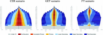
As a final step, education was introduced in the model by including education differentials in fertility and mortality, along with specific education scenarios for the future. Two education scenarios were added to the GET scenario: One scenario where educational expansion fastens (Fast Track scenario, based on the expansion of education in South Korea since the 1960s) and another scenario where it is stalled (Constant enrolment rate, meaning that countries are still able to cope with population growth).
What the scenarios mostly show is that there is a huge inertia in both demographic and education developments. Both characteristics move with age. While education is mostly acquired at younger ages, once an individual has reached a certain age, it is very unlikely that he/she will change his/her level of educational attainment, which makes the spread of improvements in the level of educational attainment in the whole population very slow. The same can be observed with fertility, a major determinant of population growth. Even in the case of a drastic reduction in fertility in a high fertility country, the population will likely continue to increase because of the large population of women in reproductive ages. This is clearly visible in China, whose fertility has been below replacement level since 1994 but the whole population of China will continue to increase until 2030 when it will peak above 1.4 billion and slowly decline thereafter (1.34 billion in 2050).
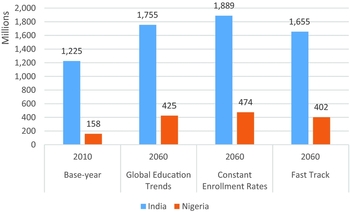
The detailed results of the projections are available in the WIC Data ExplorerFootnote 16 website and analyzed in details in Lutz et al. (Reference Lutz, Butz and KC2014a). The projection data that are also featured in Edstats,Footnote 17 a platform developed by the World Bank on education statistics are unique. The only competitor would be the datasets recently produced by Barro and Lee (Reference Barro and Lee2015) although it is more limited in terms of scope (146 countries), time (until 2040), age groups (15–64 years), and scenarios (only one trend scenario). The figures from our projection results show the combined effect of education and fertility that could lead to a much lower world population than can be imagined without taking into account levels of educational attainment. It is particularly visible in fast growing countries at the moment such as Nigeria and India (see Figure 10) for instance where an increase in education as shown by the GET scenario would imply much lower growth than other scenarios. However, as in the case of Nigeria, population momentum plays a crucial role and high population growth is unavoidable.
Total population size in 2010, and 2060 according to several education scenarios, India and Nigeria.

Another interesting feature of the projections is that it enables us to envisage how different the world would look like taking into account the population capabilities. If the world is able to develop into a global knowledge economy as shown in Figure 11 under the GET scenario and even more so under the Fast Track scenario, the outcomes in terms of global quality of life could be positively altered, not only – but also – because the human population would be less but also because it would possibly be better able to face present and future challenges due to the increasing innovative abilities of its population. Something that would be difficult to envisage if one considers a world under slow progress in education like it would be under the Constant Enrolment Rate scenario, a world possibly facing serious constraints. The comparison across time, countries or regions, and scenario can be visualized on pyramids in the graphic explorer of the WIC Data Explorer.
Population pyramids of the world in 2060 according to the constant enrolment rates, global education trend, and fast track scenarios.

The third main conclusion from the exercise is that the data illustrate that education does not jump and that it takes more decades for education gained during schooling time to translate into increased levels of education for the whole labor force. This is best illustrated when looking at the proportion with low education – aggregated from the categories no education, incomplete primary, and primary education – from 2010 to 2060 in the productive age from 20 to 64 in 26 countries in Sub-Saharan African countries where in 2010 more than three-fourth of the working age population had achieved a primary education or less. In 2060, the majority of the working age population would still have low education in 18 of these countries. Actually, only a few countries out of these 26 countries seem to have adopted a pace of education expansion able to take them out of the low education trap, e.g. Cote d'Ivoire, Sudan, Guinea Bissau, Lesotho, and Cameroon.
6. CONCLUSIONS
We have presented a new dataset on population by age, sex, and level of educational attainment for the period 1970 to 2060 (and extended to 2100) for 171 countries. This dataset was built around an initial educational distribution of the population by age and sex, with high quality criteria.
This will be developed further into the future looking into the following directions. First of all, it will be updated in 2017 to increase the country coverage and to incorporate more recent data, especially from the census rounds around 2010, which were not all available at the time of the data collection (which was completed by 2012). Furthermore, we plan to increase the time frame of the back projections going back to 1950. As mentioned earlier, this is not possible using the one and most recent dataset, and would require the choice of at least one further dataset which would have to be harmonized according to the quality criteria aforementioned. The third improvement that we have in mind is to expand the number of education categories for countries where large segments of the population are in the post-secondary education to be able to distinguish between those with a bachelor degree or any education level below bachelor degree and those with a master degree or above.
The WIC dataset has been already used in a number of scientific and action papers. First of all and as already mentioned, the modeling communities of the International Panel for Climate Change (IPCC) have utilized the different scenarios of combined education and demographic development to assess the relationships between socio-economic development and climate change [KC and Lutz (Reference K.C. and Lutz2014)]. In a similar way, and among others it was incorporated in the analysis of the role of education to reduce vulnerabilities and increase resilience by the UNDP (2014). Some researchers have also used it to model the potential economic impact of future education trajectories in poverty stricken countries [Basten and Crespo Cuaresma (Reference Basten and Cuaresma2014)]. As to the back projections [WIC (2015) and Lutz et al. (Reference Lutz, Goujon, KC and Sanderson2007)], they have been used to show the importance of education for economic growth [Lutz et al. (Reference Lutz, Cuaresma and Sanderson2008); Becker (Reference Becker2012)], over demography as shown by Crespo Cuaresma et al. (Reference Crespo, Wolfgang Lutz and Sanderson2014) in an analysis of the demographic dividend.
Although a large amount of efforts have been put into collecting and harmonizing the existing data on education, one clear caveat in our research and in actually in all reconstruction and projection exercises related to educational attainment is that we do not control for the quality of education. Hence, we consider that the 20% of women aged 20–39 years in the Czech Republic with some completed post-secondary education are by definition equivalent to the 20% with the same level of education in Chile or Fiji, whereas it is highly plausible that these groups are very heterogeneous in terms of acquired skills, and areas of specialization. The disparities in quality also exists within countries. While having knowledge about the quality of education is key as has been demonstrated for instance by Hanushek and Wößmann (Reference Hanushek and Wößmann2007), it is very difficult to implement with the reconstruction exercise (and even more so in the case of the projection exercise) and would have to be pasted on the distribution. Furthermore, it requires data that are difficult to harmonize even if using datasets that are supposed to be comparable across countries, e.g. on quality of education such as Programme for International Student Assessment (PISA), the Trends in International Mathematics and Science Study (TIMSS), and the Progress in International Reading Literacy Study (PIRLS). However, it is clear that the quality and content of education and its relevance to address the challenges that are facing humanity today are crucial.
Other interesting features that are not yet incorporated into the projections are the financial, physical, and human constraints associated with increases in developing education. At present, the scenarios are developed in an economic void, whereas many countries, especially whose with the participation in education is lagging behind at present, would not be able to implement some of the improvements intended in the scenarios, particularly the fast track scenario.
The reconstruction and projection of educational attainment constitute important exercises because they contribute to show that the changes that have occurred in the past in terms of educational attainment have participated to the major improvements and societal advancement that the world has seen in the 20th century and that can best observed in the diminishing of human mortality. The challenges that planet earth is facing today and will be increasingly facing will require innovative solutions and inventive thinking, and education will be critical.
APPENDIX
Availability of educational attainment from empirical census/survey data by country and year

Share of population aged 30 to 34 years by region that reached “universal primary”, “universal lower secondary”, and “a certain threshold of post-secondary education”, 1970 to 2010 (in percent)

Comparison of selected reconstruction efforts of levels of educational attainment