



1. Introduction
Liquid plugs forming as a result of the Plateau–Raleigh instability from a liquid film coating the inner surface of a cylindrical tube (figure 1) occur in several applications, e.g. in pulsating heat pipes as a result of phase transition (Nikolayev & Marengo Reference Nikolayev and Marengo2018), in concepts for cleaning contaminated surfaces (Zoueshtiagh, Baudoin & Guerrin Reference Zoueshtiagh, Baudoin and Guerrin2014; Khodaparast et al. Reference Khodaparast, Kim, Silpe and Stone2017), in surfactant replacement therapy (SRT), where a surfactant-rich liquid is injected into the lungs (Filoche, Tai & Grotberg Reference Filoche, Tai and Grotberg2015), and in airway occlusion (Grotberg Reference Grotberg1994, Reference Grotberg2011), typically when the mucus film lining the pulmonary airways exceeds the threshold volume for liquid unduloids (Everett & Haynes Reference Everett and Haynes1972).
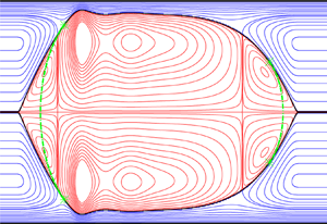
Liquid plugs (subscript  $\mathrm {1}$) enclosing a gas bubble (subscript
 $\mathrm {2}$) formed by the occlusion of a narrow cylindrical tube by a falling liquid film lining its inner surface. (a) Problem sketch and notations. The tube radius
 $R^\star$ is used as the length scale, the star superscript designating dimensional quantities; (b) travelling-state solution obtained from our model (2.13) for a vertical configuration:
 ${\textit {Ka}}=121.4$ (silicone oil II in table 1),
 $R^\star =1.5\,{\rm mm}$,
 $L=\varLambda =5.4$,
 $V_1/{\rm \pi} /R^3=2.85$,
 $M=1$,
 $d_{plug}=0.01$,
 ${\textit {Re}}_1=14.6$,
 ${\textit {Re}}_2=30.8$, where L,
 $\varLambda, V_1, M, d_{plug}$ and
 $\textit{Re}$ denote the domain length, wavelength, liquid volume, normalized gas pressure drop (2.18), pseudo-plug core radius (2.13c) and Reynolds number, respectively. Streamlines in the moving reference frame within the liquid (blue lines) and gas (red lines). Dot-dashed green lines correspond to spherical-cap reconstruction (2.14) between patching points marked by asterisks.

Properties of the fluids used in our computations. The Kapitza number,  ${\textit {Ka}}$, is defined as
 ${\textit {Ka}}=\sigma /(\rho _1 g^{1/3} \nu _1^{4/3})$, where
 $\sigma$,
 $\rho _1$ and
 $\nu _1$ denote the surface tension and the density and kinematic viscosity of the liquid, and
 $g=9.81\,{\rm m}\,{\rm s}^{-2}$ designates the gravitational acceleration.

In the current manuscript, we are mainly interested in airway occlusion, where hydrodynamical studies have focused on two key issues: (i) predicting the threshold for liquid-plug formation under increasingly realistic operating conditions, which is essential for designing effective assisted ventilation protocols (Halpern, Jensen & Grotberg Reference Halpern, Jensen and Grotberg1998); and (ii) predicting the wall stresses associated with liquid plugs, which are known to cause epithelial cell damage (Bilek, Dee & Gaver Reference Bilek, Dee and Gaver III2003). We aim to contribute to these tasks by applying the two-phase axisymmetric weighted residual integral boundary-layer (WRIBL) model of Dietze & Ruyer-Quil (Reference Dietze and Ruyer-Quil2015), which was augmented in Dietze, Lavalle & Ruyer-Quil (Reference Dietze, Lavalle and Ruyer-Quil2020) for the representation of liquid plugs.
We start by describing the state of the art on the fluid mechanics of liquid plugs, with particular attention to their occurrence in the human lung. The modelling of liquid plugs was initiated by Bretherton (Reference Bretherton1961), who predicted the shape of a long Taylor bubble (Taylor Reference Taylor1961) propagating in a liquid-filled narrow cylindrical capillary, in the absence of gravity and for a passive gas, i.e.  $\varPi _\mu =\varPi _\rho=0$, where
 $\varPi _\rho =\rho _2/\rho _1$ and
 $\varPi _\mu =\mu _2/\mu _1$ denote the gas/liquid density and dynamic viscosity ratios. This solution was based on the lubrication equations describing the thin liquid film enclosing the gas bubble, which are obtained by truncating the governing equations at order
 $\epsilon ^0$ in the long-wave parameter,
 $\epsilon =h^\star /\varLambda ^\star$ (stars will denote dimensional quantities throughout), which relates the liquid film thickness,
 $h^\star$, to the wavelength,
 $\varLambda ^\star$, of the bubble/plug arrangement (see figure 1). This lubrication solution is matched to two spherical caps at the leading and trailing ends of the bubble. Subsequent works retained the assumption of inertialess flow, but made technical improvements, such as accounting for the finite thickness of the residual film (Aussillous & Quéré Reference Aussillous and Quéré2000; Klaseboer, Gupta & Manica Reference Klaseboer, Gupta and Manica2014), or by accounting for higher-order viscous effects, via asymptotic expansions in terms of the capillary number,
 ${\textit {Ca}}=\mu _1\,\mathcal {U}_2/\sigma$, where
 $\mu _1$,
 $\mathcal {U}_2$ and
 $\sigma$ denote the liquid dynamic viscosity, the gas superficial velocity and the surface tension, and/or in terms of the long-wave parameter,
 $\epsilon$ (Park & Homsy Reference Park and Homsy1984; Jensen et al. Reference Jensen, Libchaber, Pelce and Zocchi1987). Other works accounted for the effect of gravity (Jensen et al. Reference Jensen, Libchaber, Pelce and Zocchi1987; Lasseux Reference Lasseux1995; Atasi et al. Reference Atasi, Khodaparast, Scheid and Stone2017), a contact line at the leading front of the liquid plug (Kalliadasis & Chang Reference Kalliadasis and Chang1994; Bico & Quéré Reference Bico and Quéré2001) or a flexible tube wall (Howell, Water & Grotberg Reference Howell, Water and Grotberg2000).
Lubrication models following the above-described approach have been applied to simulate liquid plugs in the pulmonary airways. For example, Suresh & Grotberg (Reference Suresh and Grotberg2005) investigated the effect of gravity on the liquid distribution within a liquid plug upstream of an inclined airway bifurcation, in order to quantify the maldistribution into the daughter airways. More recently, Fujioka et al. (Reference Fujioka, Halpern, Ryans and Gaver III2016) introduced a three-zone model for long liquid plugs, where the non-interacting leading and trailing menisci were represented via lubrication solutions from the literature (Kalliadasis & Chang Reference Kalliadasis and Chang1994; Klaseboer et al. Reference Klaseboer, Gupta and Manica2014). The authors applied their model, which compares favourably with direct numerical simulations (DNS) in regimes with negligible inertia, to study the transient evolution of pressure-driven liquid plugs, leading up to plug rupture. Throughout the manuscript, we will designate numerical simulations based on the full Navier–Stokes equations as DNS, even though these simulations do not concern turbulent flows. The authors also determined correlations for the maximum wall stresses and their spatial derivatives, in order to predict the potential for epithelial cell damage.
When inertia is not negligible, the low-dimensional representation of liquid plugs in cylindrical tubes needs to be extended beyond the lubrication approximation (Heil Reference Heil2001). For example, Aussillous & Quéré (Reference Aussillous and Quéré2000) extended the lubrication solution of Bretherton (Reference Bretherton1961) based on an empirical approach by incorporating the Weber number, which relates inertia to capillarity. A different approach was followed in Dietze et al. (Reference Dietze, Lavalle and Ruyer-Quil2020), where we introduced an augmented simplified order- $\epsilon ^2$ WRIBL model that represents the dynamics of a liquid film coating the inner surface of a cylindrical tube of radius,
 $R^\star$, in contact with a core gas flow. A repulsive source term,
 $\varPi _\varphi$, which enters the integral momentum equation (2.13a) and which will be defined in § 2 (see (2.13c) there), allows us to stabilize the liquid–gas interface when the core radius,
 $d^\star$, becomes very small, i.e.
 $d^\star =d_{plug}^\star \ll R^\star$. The source term becomes noticeable only when the liquid–gas interface evolves toward occluding the tube under the driving effect of the Plateau–Rayleigh instability, and it eventually stabilizes the solution in the form of a pseudo-plug, consisting of a liquid annulus filling almost the entire cross-section of the tube and an arbitrarily thin gas filament at the tube axis. This approach is similar to using a precursor film for simulating contact line problems with thin-film models (Thiele et al. Reference Thiele, Velarde, Neuffer and Pomeau2001). The augmented WRIBL model was introduced in the appendix of Dietze et al. (Reference Dietze, Lavalle and Ruyer-Quil2020), but never applied beyond a proof of concept. In the current manuscript, we validate it vs experiments and DNS and apply it to predict liquid plugs in the pulmonary airways.
Low-dimensional models for liquid plugs have often been used as building blocks in fluid mechanical multi-scale models representing the entire tracheobronchial tree. For example, Halpern et al. (Reference Halpern, Jensen and Grotberg1998) modelled the respiratory network by considering that the airway diameter, airway cross-section and ventilation flow rate all vary as continuous functions of the airway generation,  $n$, according to the lung architecture model of Weibel & Gomez (Reference Weibel and Gomez1962). Using this approach, the authors mimicked SRT by simulating the delivery of surfactant-rich liquid from a liquid plug propagating through the model lung, based on an inertialess low-dimensional solution for the deposited film thickness. Later, Filoche et al. (Reference Filoche, Tai and Grotberg2015) extended this work by accounting for the gravity-induced maldistribution of liquid at airway bifurcations, and investigated the effect of patient orientation on the effectiveness of SRT protocols. Ryans et al. (Reference Ryans, Fujioka, Halpern and Gaver III2016) constructed a multi-scale model of the conducting zone of the tracheobronchial tree (
 $n \le 16$) based on the lubrication model of Fujioka et al. (Reference Fujioka, Halpern, Ryans and Gaver III2016) for representing liquid plugs. This multi-scale model was used to simulate the dynamics of airway occlusion and reopening during assisted ventilation. It accounts for interactions between different airways, but not for the effect of gravity. In the current manuscript, we follow the approach of Halpern et al. (Reference Halpern, Jensen and Grotberg1998) for representing the tracheobronchial tree, but we use our augmented WRIBL model from Dietze et al. (Reference Dietze, Lavalle and Ruyer-Quil2020), which accounts for inertia, gravity, axial viscous diffusion and full dynamic coupling between liquid and gas, to represent the liquid plugs.
In addition to work on low-dimensional modelling, many studies have been dedicated to the DNS of liquid plugs, i.e. based on the full Navier–Stokes equations. We provide a brief summary of such works next, whereby we focus on studies that have demonstrated the relevance of the additional effects included in our WRIBL model, and on liquid-plug features that have been identified as critical in airway occlusion, and thus need to be accurately predicted by any low-dimensional model. Fujioka & Grotberg (Reference Fujioka and Grotberg2004) simulated pressure-driven travelling-plug solutions (TPS), i.e. solutions that do not change in the reference frame of the plug, in a plane channel for liquids used in different medical settings, i.e. Survanta (for SRT) and Perflubron (for partial liquid ventilation). The authors observed the loss of TPS, constituting the occlusion/reopening limit, at large values of the capillary number,  ${\textit {Ca}}$, and they discovered the existence of a large vortex in the reference frame of the liquid plug. Further, it was shown that the tangential wall shear stress varies greatly along the axial dimension of the liquid film and that its maximum magnitude is attained at the precursory capillary ripple preceding the front of the liquid plug, which is visible in figure 1. Zheng, Fujioka & Grotberg (Reference Zheng, Fujioka and Grotberg2007) later demonstrated for this configuration that inertia reduces the thickness of the trailing liquid film deposited by the liquid plug. Further, inertia was shown to increase the amplitude of the precursory capillary ripple, and, consequently, the maximum wall stresses. Ubal et al. (Reference Ubal, Campana, Giavedoni and Saita2008) constructed a stability diagram for pressure-driven TPS in a cylindrical tube for
 $\varPi _\mu =\varPi _\rho =0$. In a transient setting, unstable TPS can be associated with plug rupture, i.e. airway reopening. The authors also confirmed the existence of a moving-frame vortex in the liquid plug for their cylindrical configuration.
Another group of works has focused on transient DNS of the liquid-plug dynamics. Fujioka, Takayama & Grotberg (Reference Fujioka, Takayama and Grotberg2008) simulated pressure-driven liquid plugs in a cylindrical tube for  $\varPi _\mu =\varPi _\rho =0$, where the leading film thickness was imposed as a control parameter, which is representative of SRT conditions. Based on this, the authors determined how different control parameters affect the long-term fate of a liquid plug, i.e. whether the plug ruptures, attains a TPS or grows indefinitely. Further, the authors demonstrated via a dimensional analysis that inertial effects cannot necessarily be neglected in the case of airway closure, where the liquid viscosity is lower than for SRT. Finally, the authors confirmed that the precursory capillary ripple in front of the liquid plug develops the largest wall stresses and showed that the axial wall pressure derivative attains very large values there. Further, these different stress measures were shown to attain values sufficiently large to cause epithelial cell damage in the case of SRT, and to increase with increasing surface tension. Hassan et al. (Reference Hassan, Uzgoren, Fujioka, Grotberg and Shyy2011) extended the work of Fujioka et al. (Reference Fujioka, Takayama and Grotberg2008) by accounting for an active-gas phase and showed that this effect, as well as the effect of inertia, modifies the critical conditions for plug rupture. Olgac & Muradoglu (Reference Olgac and Muradoglu2013) performed similar simulations in order to mimic SRT in a subregion of the tracheobronchial tree, i.e.
 $7 \le n \le 19$, and evaluated the associated maximum wall stresses. The authors concluded that the most dangerous conditions with respect to epithelial cell damage occur in the most distal airways (farthest from the trachea).
In the context of airway occlusion, Muradoglu et al. (Reference Muradoglu, Romano, Fujioka and Grotberg2019) performed DNS of pressure-driven liquid plugs and studied the effect of a soluble surfactant. The authors showed that the surfactant reduces the maximum stress magnitudes associated with plug rupture, i.e. airway reopening, by approximately 20 %, whereas it delays plug rupture by approximately 10 %. Other authors performed DNS that account for the non-Newtonian rheology of mucus. For example, Hu, Romano & Grotberg (Reference Hu, Romano and Grotberg2020) showed that the presence of a yield stress delays plug rupture and Romano et al. (Reference Romano, Muradoglu, Fujioka and Grotberg2021) showed that the visco-elastic rheology of mucus, which in the case of cystic fibrosis becomes dominated by the elastic response, can cause a second very significant wall stress peak after initial airway occlusion, thus increasing the danger of epithelial cell damage.
We turn now to experimental investigations of liquid plugs in narrow geometries, focussing again on works related to airway occlusion. Baudoin et al. (Reference Baudoin, Song, Manneville and Baroud2013) modelled pulmonary airways via horizontal single-channel and branched microfluidic networks and studied airway reopening scenarios in trains of liquid plugs under an imposed pressure drop. The authors showed that the first plug rupture entrains and accelerates the next rupture events in the form of a cascade. Later, Hu et al. (Reference Hu, Bian, Grotberg, Filoche, White, Takayama and Grotberg2015) performed similar experiments with a viscoelastic test liquid, mimicking conditions in an  $n=12$ airway. Camassa, Ogrosky & Olander (Reference Camassa, Ogrosky and Olander2014) and Camassa, Ogrosky & Olander (Reference Camassa, Ogrosky and Olander2017) performed seminal occlusion experiments that identified the threshold for liquid-plug formation in vertical cylindrical tubes. These experiments are particularly challenging to reproduce via low-dimensional models, as high-viscosity liquids were used, where axial viscous diffusion becomes relevant. In Dietze et al. (Reference Dietze, Lavalle and Ruyer-Quil2020), we showed that accounting for this effect in our WRIBL model was necessary to capture the experimental occlusion threshold, which we predicted based on the loss of travelling-wave solutions (TWS). In the current manuscript, we will show that our augmented WRIBL model accurately captures the liquid plugs observed in these experiments.
Magniez et al. (Reference Magniez, Baudoin, Liu and Zoueshtiagh2016) studied pressure-driven liquid plugs in an individual horizontal narrow cylindrical tube, mimicking airways with  $n \ge 9$, at moderate values of
 ${\textit {Ca}}$. The authors introduced a lubrication model similar to Fujioka et al. (Reference Fujioka, Halpern, Ryans and Gaver III2016) with which they identified TPS. Then, they showed experimentally that liquid plugs evolve towards plug rupture when their initial length is shorter than the TPS, whereas they keep accumulating liquid when their initial length is longer than the TPS. Mamba et al. (Reference Mamba, Magniez, Zoueshtiagh and Baudoin2018) used the same experimental set-up, this time focussing on plug rupture under cyclic forcing in the case of an initially dry tube wall. The authors found that cyclic gas flow rate variations lead to a periodic plug motion, whereas cyclic gas pressure variations lead to a cascading reduction of the plug volume and, eventually, plug rupture. The authors caution that their study is not fully representative of mucus plug dynamics under breathing conditions. Although their forcing frequency,
 $f^\star =0.25\,{\rm Hz}$, was close to the typical breathing frequency,
 $f^\star =0.33\,{\rm Hz}$, the viscosity of the employed liquid,
 $\mu _1=5.1\times 10^{-3}\,{\rm Pa}\,{\rm s}$, was much smaller than the representative viscosity of mucus, i.e.
 $\mu _1=13\times 10^{-3}\,{\rm Pa}\,{\rm s}$ (Muradoglu et al. Reference Muradoglu, Romano, Fujioka and Grotberg2019). Later, similar experiments were performed in channels with square cross-section (Mamba, Zoueshtiagh & Baudoin Reference Mamba, Zoueshtiagh and Baudoin2019; Srinivasan, Rahatgaonkar & Khandekar Reference Srinivasan, Rahatgaonkar and Khandekar2021) or by using a visco-elasto-plastic liquid (Bahrani et al. Reference Bahrani, Hamidouche, Moazzen, Seck, Duc, Muradoglu, Grotberg and Romano2022).
We conclude our review of experimental works by discussing a series of highly sophisticated experiments that have clearly established a link between liquid plugs and epithelial cell damage (Bilek et al. Reference Bilek, Dee and Gaver III2003; Kay et al. Reference Kay, Bilek, Dee and Gaver III2004; Huh et al. Reference Huh, Fujioka, Tung, Futai, Paine, Grotberg and Takayama2007; Tavana et al. Reference Tavana, Kuo, Lee, Mosadegh, Huh, Christensen, Grotberg and Takayama2010, Reference Tavana, Zamankhan, Christensen, Grotberg and Takayama2011). In these experiments, which were initiated by Bilek et al. (Reference Bilek, Dee and Gaver III2003), real epithelial cell tissue was subjected to pressure-driven liquid plugs within micro-channels, and both the degree of cell damage, via two dies that allow distinguishing between live and dead cells, and the associated maximum magnitudes of wall stresses and their spatial derivatives, were measured. It was concluded in Kay et al. (Reference Kay, Bilek, Dee and Gaver III2004) that the maximum of the axial pressure derivative,  $\partial _{x^\star }p_{w}^\star$, which occurs near the plug front, is responsible for the main cell damage, i.e. high cell damage was observed for
 $\partial _{x^\star }p_{w}^\star \sim 0.6\,{\rm Pa}\,\mathrm {\mu }{\rm m}^{-1}$, and that the exposure time to critical stress conditions is not relevant. Interestingly, the maximum magnitude of the axial derivative of the tangential wall shear stress,
 $\partial _{x^\star }\tau _{w}^\star$, was an order of magnitude lower in these experiments. By contrast, both stress derivatives were of comparable magnitude in the lubrication model computations of Fujioka et al. (Reference Fujioka, Halpern, Ryans and Gaver III2016). In our current manuscript, we come to the same conclusion based on our WRIBL model computations, which we have validated with DNS. These results are supported by the work of Tavana et al. (Reference Tavana, Zamankhan, Christensen, Grotberg and Takayama2011), who performed DNS for conditions corresponding to their own cell damage experiments in a micro-channel, showing that
 $\partial _{x^\star }p_{w}^\star \sim 0.6\,{\rm Pa}\,\mathrm {\mu }{\rm m}^{-1}$ and
 $\partial _{x^\star }\tau _{w}^\star \sim 0.6\,{\rm Pa}\,\mathrm {\mu }{\rm m}^{-1}$ attain similar levels. The authors concluded that both quantities are linked to cell damage and showed that the level of cell damage can be greatly reduced by adding a surfactant. In Huh et al. (Reference Huh, Fujioka, Tung, Futai, Paine, Grotberg and Takayama2007), the experiments of Kay et al. (Reference Kay, Bilek, Dee and Gaver III2004) were extended by generating dynamic plug rupture events and it was shown that these events are linked to substantial epithelial cell damage.
In the current manuscript, we introduce a low-dimensional approach for predicting liquid plugs in the pulmonary airways, as well as the associated maximum wall stresses and their spatial derivatives. Our approach relies on the augmented WRIBL model of Dietze et al. (Reference Dietze, Lavalle and Ruyer-Quil2020) for the representation of liquid plugs, which we apply to track solutions via numerical continuation across the entire conducting zone of the tracheobronchial tree. In particular, we will show that this model allows us to establish a direct continuation path from TWS to TPS. Earlier studies based on thin-film models could only capture TWS. Although this allows us to predict a conservative threshold for plug formation, i.e. based on the limit point (LP) of TWS (Camassa et al. Reference Camassa, Ogrosky and Olander2014, Reference Camassa, Marzuola, Ogrosky and Vaughn2016, Reference Camassa, Ogrosky and Olander2017; Ding et al. Reference Ding, Liu, Liu and Yang2019), the properties of TPS, in particular the wall stresses they generate, and their range of existence could not be captured. We refer to Dietze et al. (Reference Dietze, Lavalle and Ruyer-Quil2020) for a thorough review of such works and mention here only works that have been published since, i.e. Camassa et al. (Reference Camassa, Marzuola, Ogrosky and Swygert2021), who studied the stability of TWS, Ogrosky (Reference Ogrosky2021a), who accounted for an additional liquid layer representing the PCL (periciliary liquid), which bathes the beating cilia responsible for mucus clearance in the conducting zone, and Ogrosky (Reference Ogrosky2021b), who studied the effect of a surfactant.
Further, our augmented WRIBL model was developed up to order  $\epsilon ^2$ in the long-wave parameter, which allows accounting for axial viscous diffusion. In Dietze et al. (Reference Dietze, Lavalle and Ruyer-Quil2020), we showed that this is important for representing the dynamics of high-viscosity annular liquid films, and this was confirmed by Ogrosky (Reference Ogrosky2021a). In the current manuscript, we will show that accounting for both inertia and axial viscous diffusion is necessary to accurately represent liquid plugs over a large liquid viscosity range, thus distinguishing our model from liquid-plug models based on the lubrication approximation.
In comparison with previous studies relying on the DNS of liquid plugs, our continuation approach distinguishes itself by enabling a low-cost high-fidelity prediction of how travelling-state solutions (TSS), i.e. TWS and TPS, evolve across the conducting zone of the tracheobronchial tree, as the airway generation,  $n$, is increased. In particular, it allows us to predict critical conditions for airway occlusion and the occurrence of wall stresses with high potential for epithelial cell damage, as well as the effect of the relevant control parameters thereon. This may prove useful in the design of drugs and protocols for the treatment of pulmonary diseases. We use the approach of Halpern et al. (Reference Halpern, Jensen and Grotberg1998) to represent the branching nature of the tracheobronchial tree, i.e. we assume that all airway properties evolve continuously with
 $n$, according to the lung architecture model of Weibel & Gomez (Reference Weibel and Gomez1962). Importantly, we track TSS that are most likely to emerge in a real system, by imposing the linearly most-amplified wavelength in our continuation calculations, which is obtained by simultaneously solving the linear stability problem. Thereby, we distinguish between convective instability (CI) and absolute instability (AI) regimes, which allows us to identify the critical airway generation for CI/AI transition. Also, our WRIBL calculations account for gravity and an active-gas phase, which were neglected in most of the above-discussed DNS studies. Gravity is not necessarily negligible, e.g. for airway generation
 $n=7$, the Bond number,
 ${\textit {Bo}}=\rho _1 g R^{\star 2}/\sigma =1.6$, where g denotes the gravitational acceleration, and where we have taken
 $\rho _1=1000\,{\rm kg}\,{\rm m}^{-3}$ for the mucus density and
 $\sigma =0.02\,{\rm N}\,{\rm m}^{-1}$ for the surface tension of mucus, according to Muradoglu et al. (Reference Muradoglu, Romano, Fujioka and Grotberg2019). And, in the presence of surfactant, this value further increases (Muradoglu et al. Reference Muradoglu, Romano, Fujioka and Grotberg2019).
Our manuscript is structured as follows. In § 2, we will introduce the employed augmented WRIBL model, followed by § 3, where we will describe the numerical approaches used to solve the model equations, i.e. linear stability analysis, numerical continuation of nonlinear TSS and transient computations of liquid-plug formation in periodic or open domains. In § 4, we will demonstrate the predictive power of the augmented WRIBL model in terms of representing liquid plugs, by comparing with experiments and DNS. In § 5, we will present our results. There, we will use numerical continuation of TSS to predict the effect of different parameters, i.e. airway generation,  $n$, airway orientation vs gravity, mucus properties, air flow rate and airway radius, on the threshold for airway occlusion (§ 5.1) and on the maximum wall stresses and spatial wall stress derivatives (§ 5.2). Conclusions will be drawn in § 6.
2. Mathematical description
We consider the flow sketched in figure 1(a), a liquid film (subscript,  $k=1$) lining the inner surface of a narrow cylindrical tube of radius,
 $R^\star$ (the star symbol denotes dimensional quantities throughout) in contact with a gas phase in the core (subscript,
 $k=2$). Both fluids are considered Newtonian with constant fluid properties and the flow as laminar. As a result of the Plateau–Rayleigh instability, the liquid can come to occlude the tube in the form of travelling plugs that enclose a gas bubble in between. Figure 1(b) represents streamlines within such a flow for a gravity-driven vertical configuration.
We denote as  $d$ the core radius, i.e. the radial distance between the tube axis and the liquid–gas interface, and as
 $h$ the liquid film thickness. We describe the flow in the framework of the long-wave approximation, which implies
 $\varepsilon =R^\star /\varLambda ^\star \ll 1$, introducing the long-wave parameter
 $\varepsilon$ and the wavelength,
 $\varLambda ^\star$, of the plug/bubble arrangement. Based on the most-amplified wavelength of the classical Plateau–Rayleigh instability,
 $\varLambda ^\star =2\sqrt {2}{\rm \pi} d_0^\star$, where the subscript zero denotes the primary flow, we obtain
 $\varepsilon =(R^\star /d_0^\star )/(2\sqrt {2}{\rm \pi} )$. As we will see, liquid-plug formation occurs for
 $d_0^\star /R^\star \sim 0.8$ in our study, yielding
 $\varepsilon \sim 10^{-1}$.
The studied flow is governed by the phase-specific (subscript  $k$) Navier–Stokes and continuity equations truncated at
 $\mathcal {O}(\varepsilon ^2)$, and written here in non-dimensional form
 \begin{gather} X_k\varepsilon\partial_t u_k+\varepsilon u_k \partial_x u_k+\varepsilon \upsilon_k \partial_r u_k={-}\varepsilon \partial_x p_k +\frac{1}{{\textit{Re}}_k}\left\{\varepsilon^2\partial_{xx} u_k+\frac{1}{r}\partial_{r} \left(r\partial_ru_k\right)\right\}+\frac{X_k^2}{{{\textit{Fr}}}^2}, \end{gather}
 \begin{gather} 0={-}\varepsilon\partial_r p_k+\varepsilon^2\frac{1}{{\textit{Re}}_k} \partial_r\left\{\frac{1}{r}\partial_{r}\left( r\upsilon_k\right)\right\}, \end{gather}
 \begin{gather} \partial_x u_k+\frac{1}{r}\partial_{r}\left( r\upsilon_k\right)= 0, \end{gather}
where  $x$ and
 $r$ denote the axial and radial coordinates,
 $u_k$,
 $\upsilon _k$ and
 $p_k$ the corresponding velocity components and pressure in phase
 $k$ and
 $t$ denotes time. Also, we have
 $X_1=1$ and
 $X_2=\varPi _u^{-1}$, and
 $\varPi _u=\mathcal {U}_2/\mathcal {U}_1$ denotes the velocity scale ratio,
 ${\textit {Re}}_k=\mathcal {U}_k\mathcal {L}/\nu _k$ denotes the phase-specific Reynolds number and
 ${\textit {Fr}}=\mathcal {U}_1/\sqrt {g\mathcal {L}}$ denotes the Froude number. Here, we have applied the following scaling:
 \begin{equation} u_k=\frac{u_k^\star}{\mathcal{U}_k},\quad \upsilon_k=\frac{\upsilon_{k}^\star}{\varepsilon\,\mathcal{U}_k},\quad x=\varepsilon\,\frac{x^\star}{\mathcal{L}},\quad r=\frac{r^\star}{\mathcal{L}},\quad t=\varepsilon\, t^\star\,\frac{\mathcal{U}_1}{\mathcal{L}}, \quad p_k=\frac{p^\star_k}{\rho_k\mathcal{U}_k^2}, \end{equation}
choosing the tube radius as the length scale,  $\mathcal {L}=R^\star$, and the phase-specific superficial velocities,
 $\mathcal {U}_k=\bar {q}_k^\star /{\rm \pi} /R^{\star 2}$, as the velocity scales, where
 $\bar {q}_k^\star$ denotes the phase-specific average cross-sectional flow rate. The truncated inter-phase coupling conditions for the normal and tangential stresses at
 $r=d$ are
 $$\begin{gather} \varepsilon p_1+\varepsilon {\textit{We}} \varepsilon^2\kappa-\frac{2 \varepsilon^2}{{\textit{Re}}_1}\partial_r \upsilon_1=\varPi_\rho\varPi_u^2\varepsilon p_2-\varPi_\mu\varPi_u\frac{2\varepsilon^2}{{\textit{Re}}_1}\partial_r \upsilon_2,\end{gather}$$
 $$\begin{gather} -(\partial_r
u_1+\varepsilon^2\,\partial_x
\upsilon_1)+2\,\varepsilon^2\,\partial_x d\left(\partial_x
u_1-\partial_r \upsilon_1\right)\nonumber\\ =
\varPi_u\varPi_\mu\{-(\partial_r
u_2+\varepsilon^2\,\partial_x
\upsilon_2)+2\,\varepsilon^2\,\partial_x
d\left(\partial_x u_2-\partial_r \upsilon_2\right)\},
\end{gather}$$
where  $\varPi _\mu =\mu _2/\mu _1$ and
 $\varPi _\rho =\rho _2/\rho _1$ denote the viscosity and density ratios,
 ${\textit {We}}=\sigma /\rho _1/\mathcal {U}_1^2/\mathcal {L}$ the Weber number and
 $\kappa$ the (truncated) surface curvature
 \begin{equation} \kappa=\frac{1}{d}-\frac{1}{2}\frac{\partial_{x}d^2}{d}-\partial_{xx}d=\kappa_\varphi-\partial_{xx}d. \end{equation}
We will also use the Kapitza number,  ${\textit {Ka}}=\sigma /(\rho _1 g^{1/3} \nu _1^{4/3})$, to characterize the working liquid. Further, we have the kinematic coupling conditions at
 $r=d$
 \begin{gather} u_1=\varPi_u u_2, \end{gather}
 \begin{gather} \upsilon_1=\varPi_u \upsilon_2, \end{gather}
 \begin{gather} X_k^{{-}1}\upsilon_k=\frac{\mathrm{d}d}{\mathrm{d}t}=\partial_t d+X_k^{{-}1}\,u_k\,\partial_xd, \end{gather}
and the radial boundary conditions
 \begin{gather} \left.{u_1}\right|_{r=R}=0,\quad \left.{\partial_ru_2}\right|_{r=0}=0, \end{gather}
 \begin{gather} \left.{\upsilon_1}\right|_{r=R}=0,\quad \left.{\upsilon_2}\right|_{r=0}=0. \end{gather}
We simplify the truncated governing equations further by applying the WRIBL technique (Kalliadasis et al. Reference Kalliadasis, Ruyer-Quil, Scheid and Velarde2012). We only sketch the procedure here, referring the reader to Dietze et al. (Reference Dietze, Lavalle and Ruyer-Quil2020) for details. First, we substitute  $p_k$ in (2.1a) via an integration of (2.1b), yielding the phase-specific boundary-layer equations,
 $\mathrm {BLE}_k$
 $$\begin{gather} \mathrm{BLE}_k:\quad
X_k\varepsilon\partial_t u_k+\varepsilon u_k \partial_x
u_k+\varepsilon \upsilon_k \partial_r
u_k={-}\varepsilon\partial_x[\left.{p_k}\right|_d]+\frac{X_k^2}{{{\textit{Fr}}}^2}\nonumber\\
-\varepsilon^2\frac{1}{{\textit{Re}}_k} \partial_{x}[
\left.{\partial_x
u_k}\right|_d]+\frac{1}{{\textit{Re}}_k}\{2\,\varepsilon^2\partial_{xx}
u_k+\partial_{rr} u_k\}.
\end{gather}$$
Next, we decompose the velocity components according to
 \begin{gather} u_k(x,r,t)=\underbrace{\hat{u}_k(x,r,t)}_{\mathcal{O}(\varepsilon^0)}+\underbrace{u_k^{(1)}(x,r,t)}_{\mathcal{O}(\varepsilon^1)}, \end{gather}
 \begin{gather} \upsilon_k(x,r,t)=\underbrace{\hat{\upsilon}_k(x,r,t)}_{\mathcal{O}(\varepsilon^0)}+\underbrace{\upsilon_k^{(1)}(x,r,t)}_{\mathcal{O}(\varepsilon^1)}, \end{gather}
introducing the leading-order velocity  $\hat {u}_k$, which is governed by
 \begin{gather} \frac{1}{r}\partial_{r}(r\partial_r\hat{u}_k)=Z_k, \end{gather}
 \begin{gather} \left.{\partial_ru_1}\right|_d=\varPi_\mu\varPi_u\left.{\partial_ru_2}\right|_d,\quad \left.{u_1}\right|_d=\varPi_u\left.{u_2}\right|_d,\quad \left.{u_1}\right|_R=\left.{\partial_ru_2}\right|_0=0, \end{gather}
 \begin{gather} 2{\rm \pi}\int_{d(x,t)}^Rr\hat{u}_1\,\mathrm{d}r=q_1(x,t),\quad 2{\rm \pi}\int_0^{d(x,t)}r\hat{u}_2\,\mathrm{d}y=q_2(x,t), \end{gather}
where  $q_k$ denotes the phase-specific cross-sectional flow rate. This leads to
 \begin{gather} \hat{u}_k=f_{ki}(r,d)\,q_i(x,t), \end{gather}
 \begin{gather} \hat{v}_1={-}\frac{1}{r}\int_r^1 \tilde{r}\partial_x\hat{u}_1 \,{\rm d}\tilde{r},\quad \hat{v}_2=\frac{1}{r}\int_0^r\tilde{r}\partial_x\hat{u}_2 \,{\rm d}\tilde{r}, \end{gather}
where  $\hat {\upsilon }_k$ is obtained via integration of (2.1c). Then, we introduce (2.8) in the
 $\mathrm {BLE}_k$ from (2.7), and combine the resulting equations via a weighted integration
 \begin{equation} \int_{d(x,t)}^R r w_1(r)\,\mathrm{BLE}_{1}\,\mathrm{d}r+\varPi_\rho\varPi_u^3\int_0^{d(x,t)} r w_2(r)\,\mathrm{BLE}_{2}\,\mathrm{d}r, \end{equation}
where the weight functions,  $w_k$, satisfy
 \begin{equation} w_k(r,d)=f_{k1}(r,d)-\varPi_u^{{-}1}f_{k2}(r,d). \end{equation}
Finally, truncating (2.11) at  $\mathcal {O}(\varepsilon ^2)$, dropping inertial corrections of order
 $\mathcal {O}({\textit {Re}}_k\varepsilon u_k^{(1)})$ and introducing the source term
 $\varPi _\varphi$, yields the final integral momentum equation rescaled by setting
 $\varepsilon =1$
 $$\begin{gather} S_i\partial_t q_i+F_{ij}q_i\partial_xq_j+G_{ij}q_iq_j\partial_xh=\frac{{\textit{We}}}{2{\rm \pi}}\partial_x\kappa+{\varPi_\varphi}+\frac{1}{2{\rm \pi}}{\textit{Fr}}^{{-}2}(1-\varPi_\rho)+\frac{1}{2{\rm \pi}}{C_i}q_i\nonumber\\ +\,{J_i}q_i\partial_xh^2+{K_i}\partial_xq_i\partial_xh+{L_i}q_i\partial_{xx}h+{M_i}\partial_{xx}q_i, \end{gather}$$
to which are added the integral continuity equations
 \begin{equation} \partial_td-\frac{1}{2{\rm \pi} d}\partial_xq_1=0,\quad \partial_td+\frac{\varPi_u}{2{\rm \pi} d}\partial_xq_2=0, \end{equation}
obtained through integration of (2.1c), with the help of (2.5c). The model coefficients  $S_i$,
 $F_{ij}$,
 $G_{ij}$,
 $C_i$,
 $J_i$,
 $K_i$,
 $L_i$ and
 $M_i$ are known functions of
 $d$ (Dietze Reference Dietze2022). Equations (2.13a) and (2.13b) constitute the 3-equation WRIBL model of Dietze et al. (Reference Dietze, Lavalle and Ruyer-Quil2020) for the three unknowns,
 $d$,
 $q_1$ and
 $q_2$.
The source term,  $\varPi _\varphi$, is designed to represent liquid pseudo-plugs
 \begin{equation} \varPi_\varphi={-}\frac{{\textit{We}}}{2{\rm \pi}}\varPi_{CRL}\exp\left[\lambda\left(1-\frac{d(x,t)}{d_{plug}}\right)\right]\partial_x\kappa_\varphi, \end{equation}
where  $\varPi _{CRL}$ sets the magnitude of
 $\varPi _\varphi$,
 $\lambda$ is a slope coefficient (
 $\lambda =1$ in all our computations) and
 $d_{plug}$ designates the core radius of a pseudo-plug. By pseudo-plug, we mean a liquid annulus that fills the entire tube cross-section except for an arbitrarily thin filament of core fluid with
 $d=d_{plug} \ll 1$ (
 $d_{plug}=0.01$ in our computations). Thanks to this approach, liquid plugs can be represented without violating the mathematical requirement of a finite core radius
 $d(x)$.
The source term,  $\varPi _\varphi$, is comparable to the so-called disjoining pressure typically used for imposing a precursor film in lubrication models for contact line problems (Thiele et al. Reference Thiele, Velarde, Neuffer and Pomeau2001). At
 $d=d_{plug}$ and
 $\varPi _{CRL}=1$,
 $\varPi _\varphi$ exactly cancels the azimuthal capillary term,
 $({{\textit {We}}}/{2{\rm \pi} })\partial _x\kappa _\varphi$, in (2.13a), which is responsible for the Plateau–Rayleigh instability, thus rendering the cylindrical surface of the pseudo-plug stable. For
 $d>d_{plug}$,
 $\varPi _\varphi <({{\textit {We}}}/{2{\rm \pi} })\partial _x\kappa _\varphi$ and the Plateau–Rayleigh mechanism remains dominant, whereas the opposite holds for
 $d< d_{plug}$. As a result, the film surface is attracted toward
 $d=d_{plug}$ from both sides. Because
 $\varPi _\varphi$ varies very sharply around
 $d_{plug}$, this effect is felt only when
 $d$ is close to
 $d_{plug}$, and it translates into a very strong repulsion of the film surface in the limit
 $d\to 0$. Moreover, the cylindrical surface
 $d=d_{plug}$ can be rendered entirely stable in the presence of a mean flow via an appropriate choice of
 $\varPi _{CRL}\ge 1$ (see § 3.1).
At the LPs of a real liquid plug,  $d{\to }0$ and
 $\partial _xd{\to }\pm \infty$. Of course, such an infinitely steep liquid–gas interface cannot be represented in the framework of the long-wave approximation. Consequently, the leading and trailing fronts of pseudo-plugs computed with our augmented WRIBL model (2.13a) are less steep than for real plugs. We will show in § 4 that this does not prevent our model from producing excellent estimates of different plug measures (see e.g. figure 5). Nonetheless, a static approximation (Lamstaes & Eggers Reference Lamstaes and Eggers2017) can improve our prediction of the plug shape. Here, following Bretherton (Reference Bretherton1961), we approximate the liquid–gas interface by a spherical cap (see e.g. figure 6), denoted by the subscript
 $sc$, in regions where the interface slope,
 $\partial _xd$, is too large for the long-wave approximation to hold, i.e. for
 $|\partial _xd|\ge \epsilon ^{max}$, whereby we choose
 $\epsilon ^{max}\sim 1$. The radius,
 $R_{sc}$, and centre,
 $x_{sc}$, of the spherical cap are obtained by requiring continuity of
 $d$ and
 $\partial _xd$ across the patching point, (
 $x_{p}$,
 $d_{p}$)
 $$\begin{gather} d_{p}=\left.{d}\right|_{x=x_{p}}\equiv\left\{R_{sc}^2-\left(x_{p}-x_{sc}\right)^2\right\}^{1/2}, \end{gather}$$
 $$\begin{gather}\left.{\partial_xd}\right|_{x=x_{p}}=\epsilon^{max}\equiv{-}\frac{x_{p}-x_{sc}}{d_{p}}. \end{gather}$$
We point out that a spherical approximation is valid only when the effect of gravity is weak over the axial length scale of the cap and liquid viscous stresses are dominated by surface tension (small capillary number,  ${\textit {Ca}}$), which turns out to be the case for typical conditions of liquid plug formation in the pulmonary airways (see figures 13d and 15c).
Our WRIBL model can be extended with a fourth evolution equation for the gas pressure at the liquid–gas interface,  ${p_2}|_d$. This is obtained by performing the operation in (2.11) with the modified weight functions,
 $\tilde {w}_k=f_{k1}(r,d)+\varPi _u^{-1}f_{k2}(r,d)$, in which case
 ${p_2}|_d$ does not cancel from (2.7) and can be solved for, yielding
 \begin{align}
2\varPi_\rho\varPi_u^2\,\partial_x[\left.{p_2}\right|_d]&={-}\tilde{S}_i\partial_t
q_i+\mbox{NLP}(x,t),\nonumber\\
\mbox{NLP}(x,t)&={-}\tilde{F}_{ij}q_i\partial_xq_j-\tilde{G}_{ij}q_iq_j\partial_xh\nonumber\\
&\quad
+\frac{{\textit{We}}}{2{\rm \pi}}\partial_{x}\kappa+\frac{1}{2{\rm \pi}}{\textit{Fr}}^{{-}2}(1+\varPi_\rho)+\frac{1}{2{\rm \pi}}{\tilde{C}_i}q_i\nonumber\\
&\quad
+{\tilde{J}_i}q_i\partial_xh^2+{\tilde{K}_i}\partial_xq_i\partial_xh+{\tilde{L}_i}q_i\partial_{xx}d+{\tilde{M}_i}\partial_{xx}q_i,
\end{align}
where the tilde distinguishes coefficients from their counterparts in the momentum equation (2.13a). Introducing the total flow rate,  $q_{tot}=q_1$+
 $\varPi _u\,q_2$, this pressure equation (2.16) can be integrated across the domain length
 $L$ (Einstein's summation convention is applied below)
 \begin{align} \Delta
p_2&=\int_0^L\partial_x[\left.{p_2}\right|_h]\mathrm{d}\kern
0.06em x=\frac{1}{2\varPi_\rho\varPi_u^2}\left\{\int_0^L
\mbox{NLP}(x,t)\,\mathrm{d}\kern 0.06em
x-\int_0^L\tilde{S}_i\partial_tq_i\,\mathrm{d}\kern 0.06em
x\right\}\nonumber\\
&=\frac{1}{2\varPi_\rho\varPi_u^2}\biggl\{\int_0^L
\mbox{NLP}(x,t)\,\mathrm{d}\kern 0.06em
x-\int_0^L\biggl(\tilde{S}_1-\frac{\tilde{S}_2}{\varPi_u}\biggr)\partial_tq_1\,\mathrm{d}\kern
0.06em
x-\partial_tq_{tot}\int_0^L\frac{\tilde{S}_2}{\varPi_u}\,\mathrm{d}\kern
0.06em x\biggr\},
\end{align}
and then used as an integral condition on the pressure drop  $\Delta p_2$, or, when
 $q_2$ is imposed, to evaluate
 $\Delta p_2$ a posteriori. For this, we introduce the normalized pressure gradient
 $M$
 \begin{equation} M=\frac{\Delta p_2}{\rho_2\,g\,L}. \end{equation}
In (2.13a), the velocity corrections,  $u_k^{(1)}$, were eliminated via truncation and an appropriate choice of the weight functions,
 $w_k$ (2.12). However, they can be reconstructed a posteriori, after having obtained a solution for
 $d$ and
 $q_k$. For this, we insert (2.8) and (2.10a) into (2.1a), (2.1b), (2.3b), (2.5a) and (2.6a), eliminate
 $p_k$ via cross-differentiation, truncate at
 $\mathcal {O}(\varepsilon ^2)$ and drop terms of
 $\mathcal {O}({\textit {Re}}_k\varepsilon u_k^{(1)})$. The resulting boundary value problem can be readily solved for
 $u_k^{(1)}$
 \begin{gather} u_1^{(1)}=C_1 r^6+C_2 r^4+C_3 r^2+C_4+\ln(r)^2\{C_5 r^2+C_6\}+\ln(r)\{C_7 r^4+C_8 r^2+C_9\}, \end{gather}
 \begin{gather} u_2^{(1)}=D_1 r^6+D_2 r^4+D_3 r^2+D_4, \end{gather}
where the coefficients,  $C_i$ and
 $D_i$, are known functions of
 $d$,
 $q_k$ and their derivatives. The cross-stream velocity corrections
 $\upsilon _k^{(1)}$ are again obtained via integration of (2.1c), using (2.8), (2.10a) and (2.19). The velocity corrections
 $u_k^{(1)}$ and
 $v_k^{(1)}$ will be useful for producing accurate predictions of the wall stresses and their spatial derivatives in §§ 4 and 5.2.
3. Numerical methods
We perform three types of numerical computations based on our WRIBL model (2.13). Linear stability calculations, which allow us to identify the most-dangerous surface structures (waves or liquid plugs) emanating from interfacial instability. Numerical continuation of TSS with the continuation software Auto07P (Doedel Reference Doedel2008) allows us to identify the threshold at which nonlinear TWS transform into TPS. And, thirdly, spatio-temporal computations using custom codes based on a finite-difference spatial discretization. In the latter case, we distinguish computations with periodicity boundary conditions on a domain spanning one wavelength,  $\varLambda$, from computations on an open domain with inlet/outlet conditions.
3.1. Linear stability analysis
We consider the primary flow of an annular liquid film of core radius,  $d_0$, and flow rate,
 $q_{10}$, in contact with a gas of flow rate,
 $q_{20}$, and perturb it in terms of
 $d$ and
 $q_k$
 \begin{gather} d=d_0+d'=d_0+\hat{d}\exp\left\{{\rm i}(kx-\omega t)\right\}, \end{gather}
 \begin{gather} q_k=q_{k0}+q_k'=q_{k0}+\hat{q}_k\exp\left\{{\rm i}(kx-\omega t)\right\}, \end{gather}
where  ${\rm i}=\sqrt {-1}$, and where we have assumed the infinitesimal perturbations,
 $d'$ and
 $q_{k}'$, grow according to exponential modes with wavenumber,
 $k$, and angular frequency,
 $\omega$. Their amplitudes,
 $\hat {d}$ and
 $\hat {q}_k$, are linked via the continuity equations (2.13b)
 \begin{equation} \hat{q}_1={-}2{\rm \pi} d_0\,\hat{d}\frac{\omega}{k},\quad \hat{q}_2=2{\rm \pi} d_0\,\varPi_u^{{-}1}\hat{d}\frac{\omega}{k}. \end{equation}
Inserting (3.1) into (2.13a), and linearizing around the primary flow, we obtain the dispersion relation
 \begin{align}
\mathrm{DR}&=i\,\omega^2\,2{\rm \pi}
d\{\varPi_u^{{-}1}S_2-S_1\}\nonumber\\ &\quad
+{\rm i}\,k\,\omega\,2{\rm \pi}
d\{-\varPi_u^{{-}1}F_{22}\,q_2+F_{21}\,q_2-\varPi_u^{{-}1}F_{12}\,q_1+F_{11}\,q_1\}\nonumber\\
&\quad +{\rm i}\,k^2\{G_{22}\,q_2^2+2\,G_{12}\,q_2\,q_1+G_{11}\,q_1^2\}\nonumber\\
&\quad -\biggl\{\omega\,C_1\,d+k\,\frac{1}{2{\rm \pi}}\partial_d
C_1\,q_1\biggr\}+\biggl\{\omega\,\varPi_u^{{-}1}C_2\,d-k\,\frac{1}{2{\rm \pi}}\partial_d
C_2\,q_2\biggr\}\nonumber\\ &\quad -{\rm
i}^2\,k^3\left\{L_1\,q_1+L_2\,q_2\right\}+{\rm
i}^2\,k^2\,\omega\,2{\rm \pi}
d\{\varPi_u^{{-}1}M_2-M_1\}\nonumber\\ &-{\rm
i}^3\,k^4\,{\textit{We}}\frac{1}{2{\rm \pi}}-{\rm
i}\,k^2\,{\textit{We}}\frac{1}{2{\rm \pi}}\frac{1}{d^2}\left\{1-\varPi_{CRL}\exp\left[\lambda\left(1-\frac{d}{d_{plug}}\right)\right]\right\}=0,
\end{align}
where we have dropped the subscript  $0$ for convenience.
The capillary term involving  ${\rm i}\,k^2\,{\textit {We}}$ is due to the azimuthal curvature of the film surface, and it includes the source term,
 $\varPi _\varphi$, introduced in (2.13c). Through
 $\varPi _{CRL}$, this term can be tuned to fully stabilize a cylindrical surface at
 $d=d_{plug}\ll 1$.
In the classical Plateau–Rayleigh configuration, where  $q_k=\varPi _\mu =\varPi _\rho =0$, assuming temporally growing modes, i.e.
 $k,\omega _i \in \mathbb {R}$ and
 $\omega =i\omega _i \in \mathbb {C}$, the cutoff wavenumber,
 $k_{c}$, is given by
 \begin{equation} k_{c}=\frac{1}{d}\left\{1-\varPi_{CRL}\exp\left[\lambda\left(1-\frac{d}{d_{plug}}\right)\right]\right\}^{1/2}. \end{equation}
In the limit  $\varPi _{CRL}=0$, our model recovers the analytical cutoff wavenumber
 $k_{c}=1/d$ for all core radii,
 $d$. By contrast, when setting
 $\varPi _{CRL}=1$, full stabilization (
 $k_{c}=0$) is achieved for
 $d/d_{plug}=1$, without affecting stability for
 $d/d_{plug} \ll 1$. This makes it possible to produce nonlinear pseudo-plug solutions with our WRIBL model, where the plug is represented via a liquid annulus filling almost the entire tube cross-section, except for a narrow cylindrical gas filament of radius
 $d\sim d_{plug}$ around the tube axis, which is stable and does not pinch.
Conditions for obtaining stable pseudo-plugs may change when there is a sufficiently strong primary flow, in which case the stability limit may be affected by inertia, in contrast to the classical Plateau–Rayleigh configuration discussed above. We discuss this based on figure 2, which represents stability calculations for spatially growing modes, i.e.  $k=k_r+{\rm i}k_i \in \mathbb {C}$ and
 $\omega \in \mathbb {R}$. Figure 2(a) compares dispersion curves of the spatial growth rate,
 $-k_i$, obtained from (3.3) with the solution of the full Orr–Sommerfeld eigenvalue problem (Hickox Reference Hickox1971), for three examples of stratified gravity-driven liquid films within a cylindrical tube. For all three working liquids, which correspond to different experiments (Dao & Balakotaiah Reference Dao and Balakotaiah2000; Piroird et al. Reference Piroird, Clanet and Quéré2011; Camassa et al. Reference Camassa, Ogrosky and Olander2014) and cover a wide
 ${\textit {Ka}}$ range, our model predictions are in good agreement with the Orr–Sommerfeld solution.
Spatial linear stability of an annular liquid film in contact with air. Symbols: WRIBL; solid lines: Orr–Sommerfeld. (a) Falling liquid film. Circles:  $R^\star =1.5\,{\rm mm}$,
 ${\textit {Ka}}=121.4$ (silicone oil II/air I in table 1),
 ${\textit {Re}}_1=15.4$,
 $M=1$; asterisks: run 13 in Dao & Balakotaiah (Reference Dao and Balakotaiah2000),
 $R^\star =3.175\,{\rm mm}$,
 ${\textit {Ka}}=3.5$ (glycerol(89 %)-water/air I),
 ${\textit {Re}}_1=0.258$,
 $M=1$, diamonds: experiment from figure 3(c) of Camassa et al. (Reference Camassa, Ogrosky and Olander2014),
 ${\textit {Ka}}=3.3\times 10^{-3}$ (silicone oil I, air I in table 1),
 $R^\star =5\,{\rm mm}$,
 ${\textit {Re}}_1=4.5\times 10^{-4}$,
 $M=1$; (b) stability of a pseudo-plug obtained with our augmented WRIBL model (2.13c). Silicone oil film from panel (a):
 $d_0=d_{plug}=0.01$,
 $\lambda =1$. Dashed:
 $\varPi _{CRL}=1$,
 $\varPi _\mu =\varPi _\rho =0$; dot-dashed:
 $\varPi _{CRL}=1.01$,
 $\varPi _\mu =\varPi _\rho =0$; solid:
 $\varPi _{CRL}=1$ (
 $-k_i$ has been multiplied by
 $10^3$).

For the low-viscosity silicone oil (blue open circles), the cutoff wavenumber  $k_{c}d_0$ is shifted with respect to the classical Plateau–Rayleigh solution,
 $k_{c}d_0=1$, as a result of the inertia-driven Kapitza instability. Thus, in the passive-core limit (
 $\varPi _\mu =\varPi _\rho =0$),
 $\varPi _{CRL}>1$ is required to fully stabilize a pseudo-plug at
 $d=d_{plug}$. We show this in figure 2(b), which represents
 $-k_i(\omega )$ curves for a pseudo-plug of
 $d=d_{plug}=0.01$. Comparing the dashed and dot-dashed curves, we see that full stabilization is achieved by changing
 $\varPi _{CRL}$ from 1 to 1.01. In the case of an active-core fluid, e.g. air, full stabilization is already achieved at
 $\varPi _{CRL}=1$ (solid curve), but the growth rate is only very slightly negative in this case (
 $-k_i$ has been multiplied by
 $10^3$ in the graph).
Above, we have used linear stability analysis to demonstrate that stable pseudo-plug solutions can be obtained with our WRIBL model (2.13). In addition, we will use linear stability calculations to identify the most-dangerous linear instability modes, i.e. those that are most likely to emerge in a real system, and thus select the nonlinear solutions that will be of interest in the next section. In such calculations, we will distinguish between CI and AI modes. We will discuss this in detail in § 3.2.
3.2. Travelling-state solutions
To construct TSS, we introduce the wave/plug celerity,  $c$, and express the space and time derivatives in (2.13b) and (2.13a) via the wave coordinate
 $\xi$
 \begin{equation} \xi=x-c\,t,\quad \partial_x=\partial_\xi,\quad \partial_t={-}c\,\partial_\xi, \end{equation}
thus transforming our system of partial differential equations into a dynamical system given by
 $$\begin{gather} d'''=\mbox{NL}(d,d',d'',q_1^{MF},q_{tot}), \end{gather}$$
 $$\begin{gather}q_1^{MF}=q_1-{\rm \pi}(R^2-d^2)\,c=\bar{q}_1-{\rm \pi}(R^2-\overline{d^2})\,c, \end{gather}$$
 $$\begin{gather}q_{tot}=q_1+\varPi_uq_2=\bar{q}_1+\varPi_u\bar{q}_2, \end{gather}$$
where primes denote differentiation with respect to  $\xi$, bars signify averaging over the wavelength
 $\varLambda$ in terms of
 $\xi$, the superscript
 $\mbox {MF}$ refers to the wave-fixed moving reference frame and where we have used (3.6b) and (3.6c) to replace derivatives
 $q^{(j)}_k$ by derivatives
 $d^{(j)}$ in (3.6a). Equations (3.6b) and (3.6c) were obtained from the phase-specific continuity equations in (2.13b). Further,
 $\bar {q}_k={\rm \pi}$ for the scaling used here.
The system is closed through the periodicity boundary conditions
 \begin{equation} {d^{(j)}}\big|_{\xi=0}={d^{(j)}}\big|_{\xi=\varLambda},\quad j=0,1,2,\end{equation}
and it is solved for fixed values of  $\bar {q}_1^\star$ (controlled via
 ${\textit {Re}}_1$), which is enforced through the integral condition
 \begin{equation} \varLambda^{{-}1}\int_0^\varLambda q_1\,{\rm d}\xi=\bar{q}_1, \end{equation}
and  $q_{tot}^\star$ (via
 ${\textit {Re}}_2$), which is imposed either explicitly, or indirectly through an integral condition on the pressure drop (2.17)
 \begin{align} \Delta p_2\,2\varPi_\rho\varPi_u^{2}=\int_0^\varLambda \mbox{NLP}(d,d',d'',d''',{q}_1^{\mbox{MF}},q_{tot})\,{\rm d}\xi-\int_0^\varLambda (\tilde{S}_1-\varPi_u^{{-}1}\tilde{S}_2)d'c\,{\rm d}\xi. \end{align}
The equation system given by (3.6) and (3.7), or by (3.6) and (3.8), is solved via numerical continuation using Auto07P (Doedel Reference Doedel2008). Figure 3 represents TSS obtained this way for the silicone oil and tube radius,  $R^\star =1.5\,{\rm mm}$, used in the experiments of Piroird et al. (Reference Piroird, Clanet and Quéré2011), only that the cylindrical tube is oriented vertically here and that we have air and not water as the core phase. The dashed red line in figure 3(a), where we have plotted the minimal core radius,
 $d_{min}$, of TSS vs the liquid volume,
 $V_1$, corresponds to the standard model, i.e.
 $\varPi _{CRL}=0$. The LP of this curve (LP1) corresponds to the occlusion bound identified in Dietze et al. (Reference Dietze, Lavalle and Ruyer-Quil2020). Its upper branch corresponds to stable TWS and its lower branch to unstable TWS, as has been demonstrated by the stability calculations of Camassa et al. (Reference Camassa, Marzuola, Ogrosky and Swygert2021). Thus, even though there is multiplicity of TWS for a fixed
 $V_1$, only TWS on the upper branch should prevail in an experiment. The lower TWS branch stops abruptly as the core radius tends to zero (
 $d_{min}\to 0$). By contrast, the solid blue curve, which corresponds to our augmented model (
 $\varPi _{CRL}=1$,
 $d_{plug}=0.01$), displays a second LP (LP2), from which a branch of TPS originates. Figure 3(b) represents selected profiles (corresponding to crosses in figure 3a) of the liquid–gas interface along this curve, illustrating the evolution from TWS (dashed curves) to a TPS (solid blue curve). The dot-dashed blue curves correspond to the spherical-cap approximation (2.14), using
 $\varepsilon ^{max}=0.75$, which allows us to represent more accurately the leading and trailing fronts of the liquid plug. We will use this approximation from here on to reconstruct these portions of TPS, i.e. starting from the patching points marked by asterisks in figure 3(b).
Transition from TWS to TPS. The TSS are based on our augmented WRIBL model (2.13a). Annular liquid film in contact with air within a vertical cylindrical tube:  ${\textit {Ka}}=121.4$ (silicone oil II and air I in table 1),
 $R^\star =1.5\,{\rm mm}$,
 $M=1$,
 $\varLambda =5.4$. (a) Minimal core radius,
 $d_{min}$, in terms of the normalized liquid volume. Solid blue:
 $\varPi _{CRL}=\lambda =1$,
 $d_{plug}=0.01$; dashed red:
 $\varPi _{CRL}=0$; (b) profiles of TSS corresponding to crosses in panel (a). Toward the tube axis:
 $V_1/{\rm \pi} /R^3=1, 2, 2.5, 2.5, 2.85$. Dot-dashed blue lines correspond to spherical-cap reconstruction (2.14) between the patching points (blue asterisks), where
 $|\partial _xd|=\epsilon ^{max}=0.75$.

In our numerical continuation of TSS, we can impose the linearly most-dangerous wavenumber,  $k=2{\rm \pi} /\varLambda =k_{max}$, which is obtained by simultaneously solving the dispersion relation (3.3) governing the linear response of the liquid film. Depending on the flow conditions, we distinguish between CI and AI modes. In the case of CI, we choose a spatial stability formulation,
 $\omega \in \mathbb {R}$,
 $k \in \mathbb {C}$, and
 $k_{max}$ corresponds to the spatially most-amplified wavenumber
 \begin{equation} \mathrm{DR}(\omega,k_{max})=0,\quad \left.{\partial_\omega k_i}\right|_{k=k_{max}}=0, \end{equation}
where the expression for  $\partial _\omega k_i$ is obtained by rearranging
 $\partial _\omega \mathrm {DR}=0$. In the case of AI, we choose a spatio-temporal stability formulation (Brevdo et al. Reference Brevdo, Laure, Dias and Bridges1999),
 $\omega \in \mathbb {C}$,
 $k \in \mathbb {C}$, and
 $k_{max}$ corresponds to the absolute wavenumber
 \begin{equation} \mathrm{DR}(\omega,k_{max})=0,\quad \frac{{\rm d}}{{\rm d}k}\left.{\mathrm{DR}(\omega,k)}\right|_{k=k_{max}}=0,\quad \left.{\frac{{\rm d}\omega}{{\rm d}k}}\right|_{k=k_{max}}=0, \end{equation}
where  ${\rm d}\omega /{\rm d}k \in \mathbb {C}$ denotes the group velocity in the wall-fixed reference frame. For most of our calculations in § 5, a CI/AI transition is observed on a given TSS branch (marked by crosses, e.g. in figure 10). The transition point can be readily identified by detecting
 $\omega _i={\rm d}\omega /{\rm d}k=0$.
The primary flow underlying the solution of (3.9a) and (3.9b) is set according to the properties of the corresponding nonlinear TSS, i.e.  $d_0=d_{VE}$ and
 $q_{20}=\bar {q}_2$ or
 $M_0=M$, depending on whether the gas flow rate (figure 10) or the gas pressure drop (figure 11) is imposed. Here,
 $d_{VE}$ is the volume-equivalent core radius
 \begin{equation} d_{VE}=\left\{1-\frac{1}{\varLambda}\int_0^\varLambda (1-d^2)\,{{\rm d}\kern0.7pt x}\right\}^{1/2}. \end{equation}
3.3. Transient periodic computations
We perform transient periodic computations to represent the dynamics of liquid-plug formation from an initially uniform liquid film. For this, our model equations (2.13a) and (2.13b) are solved by numerically advancing the solution in time, i.e. from  $t=t_{old}$ to
 $t=t_{new}$. Our equations are recast by eliminating
 $q_2$ via (3.6c)
 $$\begin{gather} \partial_tq_1+S_2\left(\varPi_u S_1-S_2\right)^{{-}1}\,\partial_tq_{tot}=\mbox{NL}(\partial_{x^j}d,\partial_{x^i}q_1)+{\varPi_\varphi\left(\varPi_u S_1-S_2\right)^{{-}1}}, \end{gather}$$
 $$\begin{gather}\partial_td=\frac{1}{2{\rm \pi}\,d}\partial_xq_1, \end{gather}$$
and then integrated over the time increment  $\Delta _t=t_{new}$-
 $t_{old}$
 $$\begin{gather} \left.{q_1}\right|_{new}-\left.{q_1}\right|_{old}+S_2\left(\varPi_u S_1-S_2\right)^{{-}1}\,\partial_tq_{tot}\,\Delta_t=\int_{t_{old}}^{t_{new}}\mbox{NL}\,{\rm d}t, \end{gather}$$
 $$\begin{gather}h_{new}-h_{old}=\int_{t_{old}}^{t_{new}}\partial_xq_1\,{\rm d}t. \end{gather}$$
The time evolution of the right-hand side terms in (3.12) is represented via the semi-implicit Crank–Nicolson approximation (Patankar Reference Patankar1980)
 $$\begin{gather} \mbox{NL}=\left.{\mbox{NL}}\right|_{old}+\frac{t-t_{old}}{\Delta_t}\left\{\left.{\mbox{NL}}\right|_{new}-\left.{\mbox{NL}}\right|_{old}\right\}, \end{gather}$$
 $$\begin{gather}\partial_xq_1=\left.{\partial_xq_1}\right|_{old}+\frac{t-t_{old}}{\Delta_t}\{\left.{\partial_xq_1}\right|_{new}-\left.{\partial_xq_1}\right|_{old}\}, \end{gather}$$
and all spatial derivatives are approximated with central finite differences. Further, it is assumed in (3.12) that the model coefficients,  $S_i$,
 $F_{ij}$,
 $G_{ij}$,
 $C_i$,
 $J_i$,
 $K_i$,
 $L_i$ and
 $M_i$ (evaluated at
 $t_{old}$), as well as
 $\partial _tq_{tot}$ are constant over the time step. The nonlinear operator
 ${\mbox {NL}}|_{new}$ of the momentum equation at
 $t_{new}=t_{old}+\Delta _t$ is linearized in terms of the dependent variables,
 $h=R-d$ and
 $q_1$, and their derivatives,
 $h^{(j)}$ and
 $q_1^{(i)}$
 $$\begin{gather} \left.{\mbox{NL}}\right|_{new}=\left.{\mbox{NL}}\right|_{old}+\frac{\partial\left.{\mbox{NL}}\right|_{old}}{\partial h^{(j)}}\big\{{h^{(j)}}\big|_{new}-{h^{(j)}}\big|_{old}\big\}\nonumber\\ +\frac{\partial\left.{\mbox{NL}}\right|_{old}}{\partial q^{(i)}}\big\{{q^{(i)}}\big|_{new}-{q^{(i)}}\big|_{old}\big\}, \end{gather}$$
where the bracketed superscripts denote the power of differentiation with respect to  $x$. The thus obtained discretized evolution equations are evaluated at the
 $N_x$-1 points of an equidistant grid spanning from
 $x=\Delta _x$ to
 $x=\varLambda$ with grid spacing
 $\Delta _x=\varLambda /(N_x-1)$. The point
 $x=0$ is excluded as it coincides with
 $x=\varLambda$ due to streamwise periodicity. The periodicity conditions
 \begin{equation} {h^{(j)}}\big|_{x=0}={h^{(j)}}\big|_{x=\varLambda},\quad{q^{(i)}}\big|_{x=0}={q^{(i)}}\big|_{x=\varLambda}, \end{equation}
are imposed directly, by making use of the nodes at and downstream of  $x=0$ in the formulation of spatial derivatives at and upstream of
 $x=\varLambda$, and vice versa. We thus obtain a linear system of
 $2(N_x-1)$ algebraic difference equations with a cyclic pentadiagonal structure (Navon Reference Navon1987) for the unknowns
 ${q_1}|_{ix}$ and
 ${h}|_{ix}$. This system is solved through lower-upper (LU) decomposition at each time step, starting from the initial condition
 \begin{equation} d(x,t=0)=d_0[1+\epsilon_{I}\sin(2{\rm \pi} x/\varLambda)],\quad q_1(x,t=0)=q_{10}\left(q_{tot}(t=0),d_0\right), \end{equation}
where  $\epsilon _{I}$ denotes the initial perturbation amplitude. Alternatively, the computation can be started from a TSS constructed with Auto07P, e.g. to study its stability.
The control parameters are  $\varLambda$,
 $q_{tot}$ and the liquid volume
 $V_1$
 \begin{equation} V_1={\rm \pi} R^2\varLambda\Big\{1-\frac{1}{2}\frac{d_0^2}{R^2}(2+\epsilon_{I}^2)\Big\}. \end{equation}
The total flow rate  $q_{tot}$ is either prescribed explicitly, or it results from an integral condition on the pressure drop (2.17). In the second case, (2.17) is recast to isolate
 $\partial _tq_{tot}$
 $$\begin{gather}
\partial_tq_{tot}\,\frac{1}{\varPi_u}\biggl\{\int_0^L
{S}_2\frac{\varPi_u\tilde{S}_1-\tilde{S}_2}{\varPi_u{S}_1-{S}_2}\,\mathrm{d}\kern
0.06em x-\int_0^L\tilde{S}_2\,\mathrm{d}\kern 0.06em
x\biggr\}=2\varPi_\rho\varPi_u^2\Delta p_2-\int_0^L
\mbox{NLP}(x,t)\,\mathrm{d}\kern 0.06em x\nonumber\\
+\int_0^L
\biggl(\tilde{S}_1-\frac{\tilde{S}_2}{\varPi_u}\biggr)\mbox{NL}(x,t)\,\mathrm{d}\kern
0.06em x, \end{gather}$$
where  $\partial _tq_1$ has been eliminated via (3.11) in the limit
 $\varPi _{CRL}=0$, and then used to update
 $q_{tot}$ at each time step
 \begin{equation} \left.q_{tot}\right|_{new}=\left.q_{tot}\right|_{old}+\left.\partial_tq_{tot}\right|_{old}\,\Delta_t. \end{equation}
Figure 4 represents results of a transient periodic computation for parameters according to figure 3. In particular, we have set  $V_1/{\rm \pi} /R^3=2.85$, which lies far beyond the occlusion limit of TSS in figure 3(a). As shown in figure 4(b), our transient periodic computation, which was started from a virtually uniform film (
 $\epsilon _{I}=0.015$), evolves toward the TSS, represented here with a dashed blue profile and marked by a blue cross on the TPS branch in figure 3(a). Thus, we expect this branch to be representative of liquid plugs forming as a result of interfacial instability in a real system (comparisons with experiments are reported in § 4). The dot-dashed green curves in figure 4(a) correspond to the converged values for the instantaneous Reynolds numbers,
 $\bar {q}^\star _1/\nu _1$ and
 $\bar {q}^\star _2/\nu _2$, obtained from our own transient periodic DNS (which will be introduced in figure 6b), using the solver Gerris (Popinet Reference Popinet2009). The time traces of
 $\bar {q}^\star _1/\nu _1$ and
 $\bar {q}^\star _2/\nu _2$ obtained from our transient periodic WRIBL computation (solid and dashed black curves) converge to these values (more comparisons with DNS are reported in § 4).
Transient periodic computation of a liquid plug forming from an initially quasi-uniform film. Parameters according to figure 3:  $V_1/{\rm \pi} /R^{3}=2.85$,
 $\epsilon _{I}=0.015$. (a) Time traces of the instantaneous Reynolds numbers,
 $\bar {q}^\star _k/\nu _k$, with
 $\bar {q}_k=\varLambda ^{-1}\int _0^\varLambda q_k\,{{\rm d}\kern0.7pt x}$, in the liquid (solid) and gas (dashed). Dot-dashed green lines: final values for the DNS in figure 6(b); (b) profiles corresponding to crosses in panel (a) (solid) and to the TSS in figure 3(b) (dashed).

3.4. Open-domain computations
To represent the spatio-temporal evolution of liquid plugs, we apply the numerical procedure discussed in the previous section to an open domain with inlet and outlet conditions at  $x=0$ and
 $x=L$. Inlet conditions are set by prescribing
 $d$ and
 $q_1$ at the first two grid points (
 $i_x=1,2$) based on the primary flow
 $$\begin{gather} \left.d\right|_{i_x=1}=\left.d\right|_{i_x=2}=d_0, \end{gather}$$
 $$\begin{gather}\left.q_1\right|_{i_x=1}=\left.q_1\right|_{i_x=2}=q_{10}\left[1+F(t)\right]. \end{gather}$$
The function  $F(t)$ in (3.20b) allows us to apply a tailored inlet forcing
 \begin{equation} F(t)=\epsilon_1\sin(2{\rm \pi}\,f\,t)+\epsilon_2 \sum_{k=1}^{N} \sin(2{\rm \pi}\,k\,\Delta f\,t+\varphi_{rand}),\quad \Delta f=2\,f_{c}/N. \end{equation}
The first term constitutes a harmonic perturbation of frequency,  $f$, and the second one mimics white noise through a series of
 $N=1000$ Fourier modes that are shifted by a random phase shift,
 $\varphi _{rand}=\varphi _{rand}(k)\in [0,2{\rm \pi} ]$, and that span a frequency range of twice the linear cutoff frequency,
 $f_{c}$ (Chang, Demekhin & Kalaidin Reference Chang, Demekhin and Kalaidin1996). All our computations were run with the same
 $\varphi _{rand}(k)$ number series, which was generated once and for all with the pseudo-random number generator RandomReal in Mathematica (2014). The strength of the two terms in (3.21) is determined through their amplitudes,
 $\epsilon _1$ and
 $\epsilon _2$. When
 $\epsilon _1=0$, the inlet perturbation consists of only white noise. This setting will be used to simulate the noise-driven formation of liquid plugs, as it would occur in an experiment.
At the outlet, we apply boundary conditions inspired by those of Richard, Ruyer-Quil & Vila (Reference Richard, Ruyer-Quil and Vila2016), which ensure that liquid is always sufficiently drained from the domain, by introducing two downstream ghost nodes at  $i_x=N_x+1$ and
 $i_x=N_x+2$
 $$\begin{gather} \left.d\right|_{i_x=N_x+1}=\left.d\right|_{i_x=N_x+2}=\left.d\right|_{i_x=N_x}, \end{gather}$$
 $$\begin{gather}\left.q_1\right|_{i_x=N_x+1}=q_{10}\frac{q_{10}^{PG}(\left.d\right|_{i_x=N_x})}{q_{10}^{PG}(d_0)}, \end{gather}$$
where  $q_{10}^{PG}(d)=q_{10}(\varPi _\rho =\varPi _\mu =0,d)$ is the passive-gas limit of the primary flow rate
 $q_{10}$ for a given
 $d$, which is known analytically. Our computations are started from the initial condition
 \begin{equation} d(x,t=0)=d_0,\quad q_1(x,t=0)=q_{10}. \end{equation}
We point out that no information for the interface height in the second downstream ghost cell ( $d|_{i_x=N_x+2}$ in our case) was given in Richard et al. (Reference Richard, Ruyer-Quil and Vila2016). Our choices for
 $d|_{i_x=1}$ (3.20) and
 $d|_{i_x=N_x+2}$ (3.22) were guided by numerical convenience. The twice removed ghost cells only affect the discretized form of the third derivative,
 $\partial _{xxx}d$, which is negligible at the inlet. At the outlet, the flow is dominated by the imposed flow rate,
 $q_1|_{i_x=N_x+1}$, and, thus, the effect of
 $d|_{i_x=N_x+2}$ is weak.
4. Validation vs DNS and experiments
We validate our approach for computing liquid plugs by confronting our WRIBL model (2.13) with experiments and DNS. We start with the configuration from figure 3(a), which corresponds to silicone oil II in table 1, subject to an aerostatic pressure drop ( $M=1$). Figure 5 represents TSS in terms of two important measures, i.e. the plug speed,
 $c$, and the gas Reynolds number,
 ${\textit {Re}}_2$, which quantifies the entrained gas flow rate. As discussed in figure 3(a), liquid-plug solutions lie beyond LP1 on the solid blue curves in figure 5(a,b), which represent our WRIBL predictions. The green squares in the same graphs mark data points obtained via transient periodic DNS with Gerris (see Dietze et al. (Reference Dietze, Lavalle and Ruyer-Quil2020) for details of such runs), evidencing very good agreement with the WRIBL model. For the low-viscosity liquid considered here,
 ${\textit {Re}}_1$ is quite large, and, thus, inertia is not negligible. This is evidenced by the substantial difference (approximately 25 %) between our full-model predictions (solid blue curves) and the black dashed curves, which represent the inertialess limit of our WRIBL model (
 $S_k=F_{kj}=G_{kj}=0$ in (2.13)).
The TSS from figure 3 (curves) compared with our own DNS (symbols) using Gerris (Popinet Reference Popinet2009):  ${\textit {Ka}}=121.4$,
 $R^\star =1.5\,{\rm mm}$,
 $M=1$,
 $\varLambda =5.4$. Solid blue curve: full model (2.13), dot-dashed black curve: inertialess limit (
 $S_k=F_{kj}=G_{kj}=0$). (a) Plug celerity
 $c$; (b) gas Reynolds number,
 ${\textit {Re}}_2$, quantifying the gas flow rate transported by the gas bubbles in between two liquid plugs.

Figure 6 shows streamlines in the moving reference frame for one of the liquid-plug solutions from figure 5 ( $V_{l}/{\rm \pi} /R^3=2.85$), as obtained from our WRIBL model (figure 6a) and our DNS (figure 6b). Our model captures all relevant flow features, in particular the toroidal vortex within the liquid plug (Ubal et al. Reference Ubal, Campana, Giavedoni and Saita2008) and the three main toroidal vortices within the gas bubble. The shape of the liquid–gas interface is predicted accurately in the thin portion of the liquid film, whereas agreement deteriorates in the steepest parts of the leading and trailing fronts of the liquid plug. In these regions, the spherical-cap approximation (2.14) allows us to recover good agreement (dashed green lines).
The TPS forming in a vertical cylindrical tube. Streamlines in the reference frame moving with the plug speed,  $c$. Parameters according to figure 3(a):
 $\varLambda =5.4$,
 $V_1/{\rm \pi} /R^3=2.85$,
 $M=1$. (a) Transient periodic computation with our augmented WRIBL model (2.13):
 ${\textit {Re}}_1=30.8$,
 ${\textit {Re}}_2=14.6$,
 $c^\star =0.31\,{\rm m}\,{\rm s}^{-1}$. Dashed green lines correspond to spherical-cap approximation (2.14) between patching points (marked by green asterisks), using
 $\varepsilon ^{max}=0.75$; (b) periodic DNS with Gerris:
 ${\textit {Re}}_1=30.4$,
 ${\textit {Re}}_2=14.4$,
 $c^\star =0.30\,{\rm m}\,{\rm s}^{-1}$.

In figure 7(a), the solid black line represents the thus reconstructed liquid–gas interface for the system in figure 6 (crosses mark patching points), evidencing good agreement with the DNS profile (green line with open circles). The other three panels in figure 7 compare spatial profiles of different quantities related to the stress field at the tube wall. We start with the excess pressure  $\Delta p_{w}$
 \begin{equation} \Delta p_{w}=\frac{\Delta p_{w}^\star}{\rho_1\mathcal{U}_1^2},\quad \Delta p^\star_{w}=\left.{p^\star}\right|_{r^\star = R^\star}-\left.{p^\star}\right|_{r^\star = 0}, \end{equation}
which is obtained by integrating (2.1b), substituting (2.8), truncating at order  $\mathcal {O}(\varepsilon ^2)$, introducing (2.10b) and setting
 $\varepsilon =1$. As shown in figure 7(b), our WRIBL model (solid curves) accurately predicts both the
 $\Delta p_{w}$ profile and its maximum absolute value compared with the DNS (open green circles). The segment between the apex of the spherical cap (marked by plus sign) and the start of the pseudo-plug (marked by filled diamond) is not drawn, as it has no physical meaning.
Liquid stresses at the tube wall,  $r=1$, within a TPS. Parameters according to figure 6. Open green circles: DNS; solid black lines: WRIBL model. (a) Liquid–gas interface, showing gas bubble in between two liquid plugs; (b) pressure difference across the tube,
 $\Delta p_{w}$ (4.1); (c) axial wall shear stress derivative,
 $\partial _x\tau _{w}$, according to (4.2b); (d) axial wall pressure derivative,
 $\partial _x p_{w}$, according to (4.2a). Crosses mark patching points for spherical-cap reconstruction (2.14), using
 $\varepsilon ^{max}=0.75$, plus signs mark apex of spherical cap and diamonds mark limits of pseudo-plug.

Experiments of Kay et al. (Reference Kay, Bilek, Dee and Gaver III2004) and Tavana et al. (Reference Tavana, Zamankhan, Christensen, Grotberg and Takayama2011) have shown that liquid-plug-induced epithelial cell damage is controlled by the magnitude of the axial derivatives of wall pressure,  $p_{w}$, and wall shear stress,
 $\tau _{w}$
 \begin{gather} \partial_x p_{w}=\partial_x[{p_1}]_{r=1}={\textit{Re}}_1^{{-}1}\Big[\frac{1}{r}\partial_r\left(r\partial_r u_1\right)\Big]_{r=1}+{\textit{Fr}}^{{-}1}, \end{gather}
 \begin{gather} \tau_{w}=\left.\partial_r{u_1}\right|_{r=1},\quad \partial_x\tau_{w}=\partial_x\left[\partial_r{u_1}\right]_{r=1}, \end{gather}
where (4.2a) is obtained by evaluating (2.1a) at  $r=1$ (and setting
 $\varepsilon =1$), and where
 $u_1$ is reconstructed according to (2.8), using (2.10a) and (2.19), which ensures consistency at order
 $\mathcal {O}(\varepsilon ^2)$. Figure 7(c,d) plots profiles of
 $\partial _x\tau _{w}$ and
 $\partial _x p_{w}$ obtained from our WRIBL model (solid curves) based on (4.2b) and (4.2a), in comparison with our DNS predictions (green curves with open circles). Our WRIBL model predicts the spatial variation and the maximum magnitude of both quantities, in good agreement with the DNS.
All three quantities,  $\Delta p_{w}$ (figure 7b),
 $\partial _x\tau _{w}$ (figure 7c) and
 $\partial _x p_{w}$ (figure 7d), exhibit pronounced extrema around the first capillary trough preceding the leading front of the liquid plug. Also,
 $\partial _x\tau _{w}$ and
 $\partial _x p_{w}$ change sign over a very short length scale in this region, implying a temporally oscillatory stress field during the passage of a liquid plug. Spatio-temporal variations increase the potential of mechanical damage to epithelial cells in the pulmonary airways (Romano et al. Reference Romano, Muradoglu, Fujioka and Grotberg2021). In § 5.2, we will use our WRIBL predictions obtained from (4.1), (4.2b) and (4.2a), and the corresponding time derivatives,
 $\partial _t\tau _{w}=-c\partial _x\tau _{w}$ and
 $\partial _tp_{w}=-c\partial _xp_{w}$, to assess the potential for epithelial cell damage linked to TPS under representative flow conditions in the conducting zone of the tracheobronchial tree.
Further validation of our WRIBL model (2.13) is provided in figure 8, where we have reproduced numerically the experiment in figure 3(c) of Camassa et al. (Reference Camassa, Ogrosky and Olander2014), who studied liquid-plug formation in a narrow vertical tube, using a high-viscosity liquid (silicone oil I in table 1) in contact with air.
Highly viscous falling liquid film in contact with air:  ${\textit {Ka}}=3.3\times 10^{-3}$ (silicone oil I, air in table 1),
 $R^\star =5\,{\rm mm}$,
 ${\textit {Re}}_1=4.5\times 10^{-4}$,
 $M=1$. (a) Experiment from figure 3(c) of Camassa et al. (Reference Camassa, Ogrosky and Olander2014), reproduced here with permission from Cambridge University Press. (b) Open-domain WRIBL computation (true to scale) using inlet noise (3.21):
 $\epsilon _1=0$,
 $\epsilon _2=10^{-4}$. Leading and trailing portions of the liquid plugs were reconstructed with the spherical-cap approximation (2.14), using
 $\epsilon ^{max}=0.68$.

Our WRIBL computation (figure 8b) was performed on an open domain, applying the noisy inlet perturbation (3.21) to mimic experimental noise. Occlusion in the present case occurs according to scenario I in Dietze et al. (Reference Dietze, Lavalle and Ruyer-Quil2020), i.e. the liquid Reynolds number,  ${\textit {Re}}_1=4.5\times 10^{-4}$, lies beyond the LP of the linearly most-amplified TWS, and liquid plugs form as a result of surface waves emerging from linear wave selection. This limit point is marked by LP1 in figure 9(a), which represents TSS at
 $f=f_{max}$, where
 $f_{max}$ denotes the spatially most-amplified frequency obtained from linear stability analysis. Comparing the upper panel (experiment) and lower panel (WRIBL) in figure 8, we conclude that our model correctly represents this occlusion regime. In particular, the spatial evolution of precursory surface waves, their pinch-off to form liquid plugs (subsequently convected downstream) and the number and shape of these plugs, are predicted quite well.
The TSS at  $f=f_{max}$ and
 $M=1$ obtained with our WRIBL model (2.13) for the configuration in figure 8. Solid blue curves with circles: full model; dot-dashed black:
 $J_k=K_k=L_k=M_k=0$ in (2.13). Filled black diamonds mark AI limit. Lower branch beyond LP2 in panel (a) corresponds to TPS, which are compared with experiments (filled red squares) from figures 3(c) (
 ${\textit {Re}}_1=4.5\times 10^{-4}$) and 3(d) (
 ${\textit {Re}}_1=6.22\times 10^{-4}$) of Camassa et al. (Reference Camassa, Ogrosky and Olander2014). (a) Minimal core radius; (b) wavelength; (c) wave/plug speed; (d) plug profiles corresponding to cross and asterisk in panels (a–c). Solid:
 ${\textit {Re}}_1=4.5\times 10^{-4}$,
 $f^\star _{max}=0.145\,{\rm Hz}$; dashed:
 ${\textit {Re}}_1=6.22\times 10^{-4}$,
 $f^\star _{max}=0.155\,{\rm Hz}$.

Further, we show in figure 9 that several liquid-plug measures from the experiment can be predicted accurately based on TSS at  $f=f_{max}$ obtained with our WRIBL model. Both the wavelength,
 $\varLambda$ (combined length of liquid plug and gas bubble), represented in figure 9(b), and the plug speed,
 $c=\varLambda f_{max}$, represented in figure 9(c), lie within the experimental error bars (experimental points are marked by filled squares), which were determined graphically from the variation of
 $\varLambda$ between different plug/bubble pairs in figure 3(c) of Camassa et al. (Reference Camassa, Ogrosky and Olander2014). Crosses and asterisks on the TSS branches in figure 9(a–c) mark the experimental conditions corresponding to figure 3(c,d) in Camassa et al. (Reference Camassa, Ogrosky and Olander2014), whereby the former figure is reproduced here in figure 8(a).
The dot-dashed black curves in figure 9(a–c) represent TSS obtained in the absence of axial viscous diffusion, i.e. when setting  $J_k=K_k=L_k=M_k=0$ in (2.13). In this limit, agreement with the experiments is greatly deteriorated. Thus, accounting for axial viscous diffusion, by developing our WRIBL model up to order
 $\epsilon ^2$, has proven necessary in order to accurately capture liquid plugs of highly viscous liquids.
Finally, we point out that our open-domain computation in figure 8(b) was run with an imposed total flow rate  $q_{tot}$, corresponding to the TPS at
 $M=1$ in figure 9(a). For this high-viscosity working liquid, gas–liquid coupling is very weak (
 $\varPi _\mu =1.4\times 10^{-6}$) and thus imposing
 $M=1$ via (2.17) requires a very fine grid resolution around the liquid plug, which is prohibitive in open-domain computations.
5. Results: application to airway occlusion
We apply our WRIBL model (2.13) to study liquid-plug formation by a mucus film lining the inner surface of a respiratory airway. We assume a mucus rheology corresponding to healthy conditions, where neither viscoelasticity (Choudhury et al. Reference Choudhury, Filoche, Ribe, Grenier and Dietze2023) nor shear thinning (Chatelin et al. Reference Chatelin, Anne-Archard, Murris-Espin, Thiriet and Poncet2017) play a significant role. In particular, our computations are based on a Newtonian model mucus according to Muradoglu et al. (Reference Muradoglu, Romano, Fujioka and Grotberg2019), i.e. mucus I in table 1. For the gas phase, we assume ambient air, i.e. air I in table 1.
We focus on the conducting zone of the human respiratory network, i.e. the first 16 airway generations according to the lung architecture model of Weibel & Gomez (Reference Weibel and Gomez1962)
 $$\begin{gather} R^\star = R^\star_{\textit{Weib}}=R^\star_0\,2^{-({n}/{3})}, \end{gather}$$
 $$\begin{gather}L^\star = L^\star_{\textit{Weib}}=L^\star_0\,2^{-({n}/{3})}, \end{gather}$$
 $$\begin{gather}{\textit{Re}}_2={\textit{Re}}^{\textit{Weib}}_2={\textit{Re}}_{2 0}\,2^{-({2}/{3})n}=\frac{Q^\star_{20}}{{\rm \pi} R_0^\star\nu_2}\,2^{-({2}/{3})n}, \end{gather}$$
where  $n$ denotes the airway generation,
 $R^\star$ and
 $L^\star$ the radius and length of the airway,
 $Q^\star _2$ and
 ${\textit {Re}}_2$ the corresponding gas flow rate and gas Reynolds number and the subscript
 $0$ refers to the trachea, i.e.
 $n=0$, for which we set
 $R^\star _0=9\,{\rm mm}$ and
 $L^\star _0=120\,{\rm mm}$, according to a typical adult (Weibel & Gomez Reference Weibel and Gomez1962).
In the current manuscript, we do not account for the time variation of the air flow rate during the breathing cycle. Instead, we set a time-constant tracheal gas flow rate, which is based on the reference value  $Q^\star _{2 0}=\pm V^\star _{T}\,f^\star _{T}=\pm 2.5\times 10^{-4}\,{\rm m}^3\,{\rm s}^{-1}$, with a tidal volume,
 $V^\star _{T}=500\times 10^{-6}\,{\rm m}^3$, and a tidal frequency,
 $f^\star _{T}=0.5\,{\rm Hz}$, according to typical settings for assisted ventilation (Halpern et al. Reference Halpern, Jensen and Grotberg1998), yielding
 ${\textit {Re}}_{20}=\pm 590$. Based on this, the gas flow is always laminar for generations
 $n>2$, and we restrict our investigation to this range, as our WRIBL model does not account for turbulence.
The sign of  $Q^\star _{2 0}$ and
 ${\textit {Re}}_{20}$ allows us to distinguish between situations where the gas flow is oriented in the direction of gravity (
 $Q^\star _{2 0},{\textit {Re}}^\star _{2 0}>0$) or opposite to gravity (
 $Q^\star _{2 0},{\textit {Re}}^\star _{2 0}<0$). We will designate these as co-current and counter-current configurations throughout. Due to the branching nature of the lung architecture, two airways of the same generation can be oriented in opposite directions, and, thus, the co- and counter-current configurations can occur both during expiration and inspiration. Of course, the direction of the gas flow is relevant only when gravity plays a role, and we will show that this is the case here. Strictly speaking, our WRIBL model, which is based on an axisymmetric formulation (2.13), is valid only for airways aligned with gravity, and we will focus on this situation. Thus, we cannot account for cross-stream gravity, which can lead to asymmetric liquid distribution about the airway equator (Suresh & Grotberg Reference Suresh and Grotberg2005). For this, a full three-dimensional model is required.
Further, we neglect the effect of beating cilia lining the airway walls, which are responsible for mucociliary clearance (Spagnolie Reference Spagnolie2015), as well as the periciliary liquid (PCL) in which they are immersed. These effects are assumed to be negligible for conditions in the vicinity of liquid-plug formation. For reference, the thickness of the PCL layer is  $h_{PCL}^\star \sim 8\,\mathrm {\mu }{\rm m}$ for
 $n=16$, i.e.
 $h_{PCL}/R\sim 4\,\%$. Finally, we assume the inner surface of the airways to be perfectly cylindrical.
5.1. Liquid-plug formation based on TSS
We apply the numerical continuation procedure introduced in § 3.2 to advance TSS in terms of the airway generation  $n$ (see e.g. figure 10). For this, we assume that all quantities evolve continuously with
 $n$ (Halpern et al. Reference Halpern, Jensen and Grotberg1998), based on the lung architecture model (5.1) of Weibel & Gomez (Reference Weibel and Gomez1962). In particular, we are interested in predicting the transition from TWS to TPS, which allows us to identify in what airway generation liquid plugs may arise. In generations where TPS do not exist, plug formation is highly unlikely, even in a transient setting. In addition to the airway generation,
 $n$, there is one other free control parameter in our problem, for which we choose the liquid holdup,
 $h_{VE}=h_{VE}^\star /R^\star$
 \begin{equation} h_{VE}=1-d_{VE}, \end{equation}
which controls the thickness of the mucus film. This parameter can increase significantly in the case of mucus overproduction or impeded mucociliary clearance caused by respiratory diseases (Fahy & Dickey Reference Fahy and Dickey2010).
Airway occlusion under imposed gas flow rate for different  $h_{VE}$. Linearly most-dangerous TSS vs airway generation
 $n$ based on lung architecture (5.1) of Weibel & Gomez (Reference Weibel and Gomez1962):
 ${\textit {Ka}}=30.6$ (mucus I and air I in table 1),
 ${\textit {Re}}_{20}=\pm 590$,
 $k=k_{max}$,
 $R^\star =R^{\star }_{\textit{Weib}}$,
 ${\textit {Re}}_2={\textit {Re}}_2^{\textit{Weib}}$. Crosses mark transition between CI, where
 $\omega _i=\partial _\omega k_i=0$ is imposed (3.9a), and AI, where
 ${\rm d}\omega /{\rm d}k=0$ (with
 $k$,
 $\omega \in \mathbb {C}$) is imposed (3.9b). Filled circles to open diamonds:
 $h_{VE}=0.4$, 0.3, 0.267, 0.24, 0.2 and 0.15. (a,c) Co-current configuration:
 ${\textit {Re}}_{20}=590$,
 $M_{dry}<0$; (b,d) counter-current configuration:
 ${\textit {Re}}_{20}=-590$,
 $M_{dry}>0$. (a,b) Minimum core radius; (c,d) normalized pressure drop, where
 $M_{dry}$ (5.3) corresponds to dry airways (
 $h_{VE}=0$).

Airway occlusion under imposed pressure drop for different values of the liquid holdup,  $h_{VE}$. Linearly most-dangerous TSS vs airway generation,
 $n$, based on lung architecture (5.1) of Weibel & Gomez (Reference Weibel and Gomez1962):
 ${\textit {Ka}}=30.6$ (mucus I and air I in table 1),
 $M/M_{dry}=20$,
 ${\textit {Re}}_{20}^{dry}=590$ (
 $M_{dry}<0$),
 $k=k_{max}$,
 $R^\star =R^{\star }_{\textit{Weib}}$. Filled circles to open diamonds:
 $h_{VE}=0.4$, 0.3, 0.267, 0.24, 0.2 and 0.15. (a) Minimum core radius; (b) normalized gas Reynolds number.
 $M_{dry}$ (5.3) and
 ${\textit {Re}}_2^{dry}$ correspond to dry airways (
 $h_{VE}=0$) in the absence of gravity (
 ${\textit {Fr}}^{-1}=0$). The LPs mark onset of TPS. Crosses mark transition between CI, where
 $\omega _i=\partial _\omega k_i=0$ is imposed (3.9a), and AI, where
 ${\rm d}\omega /{\rm d}k=0$ (with
 $k$,
 $\omega \in \mathbb {C}$) is imposed (3.9b).

In our calculations, we track the linearly most-dangerous TSS by setting  $k=k_{max}$, where
 $k_{max}$ is the most-dangerous wavenumber, as obtained by simultaneously solving the linear stability problem (3.9). Thus, for each airway generation, we obtain the TSS most likely to emerge in a real system, and we have checked that the corresponding most dangerous wavelength,
 $\varLambda _{max}=2{\rm \pi} /k_{max}$, satisfies
 $\varLambda _{max} \le L_{\textit{Weib}}$, i.e. that the most-dangerous TSS fits into the typical length of the considered airway generation (see figure 12, which will be introduced later). Further, our spatio-temporal stability formulation introduced in § 3.2 allows us to distinguish between: (i) CI, where we set
 $\omega _i=\partial _\omega k_i=0$ via (3.9a), and
 $k_{max}$ corresponds to the linear mode with maximum spatial growth rate, and (ii) AI, where we set
 ${\rm d}\omega /{\rm d}k=0$ via (3.9b), and
 $k_{max}$ corresponds to the absolute mode, i.e. a perturbation growing in time at fixed axial position,
 $x$. The TPS in the AI regime are particularly dangerous, as the linear perturbation in that case cannot be advected out of the airway, and plug formation is thus more likely in a transient setting. Therefore, the CI/AI transition is highlighted by crosses in all figures of the current section, i.e. figures 10–16.
Length scales of TSS from figure 10, as compared with the airway length,  $L_{\textit{Weib}}$ (5.1). (a,b) Relative distance of propagation,
 $L_{T}/L_{\textit{Weib}}$, during half of one breathing period, 1/
 $f_{T}$, where
 $L_{T}=c$/2/
 $f_{T}$; (c,d) relative wavelength,
 $\varLambda /L_{\textit{Weib}}$. (a,c) Co-current:
 ${\textit {Re}}_{20}=590$; (b,d) counter-current:
 ${\textit {Re}}_{20}=-590$.

Figure 10 represents TSS vs the airway generation  $n$ for imposed
 $R^\star =R^\star _{\textit{Weib}}$ and
 ${\textit {Re}}_{2}={\textit {Re}}_{2}^{\textit{Weib}}$, according to (5.1), for different values of the liquid hold up,
 $h_{VE}$. Here, we confront the co-current (
 ${\textit {Re}}_{20}=590$, figure 10a,b) and counter-current (
 ${\textit {Re}}_{20}=-590$, figure 10c,d) configurations. Figure 10(a) represents TSS in terms of the minimum core radius,
 $d_{min}$ (solid curves). Upon decreasing
 $h_{VE}$ (from
 $h_{VE}=0.4$ to
 $h_{VE}=0.2$), the critical generation for TPS formation (LPs, marked by symbols) shifts significantly toward distal airways (from
 $n=6$ to
 $n=14$). At the same time, the CI/AI transition (marked by crosses) increasingly shifts from the TPS branch to the TWS branch, making liquid-plug formation in a transient setting more and more likely. In particular, for
 $h_{VE}\le 0.267$, the entire TPS branch lies in the AI regime. We point out that the observed multiplicity of TSS at fixed
 $h_{VE}$ and
 $n$ is similar to the one discussed in figure 3(a). It is quite probable that the TWS on the intermediate branches between the upper LP and the TPS are unstable here as well. To check this rigorously, the approach of Camassa et al. (Reference Camassa, Marzuola, Ogrosky and Swygert2021) for investigating the stability of TWS needs to be applied to the continuation results in figure 10(a), where the continuation parameter is different. This is outside the scope of the current manuscript.
According to figure 10(c), the TPS from figure 10(a) are associated with a spectacular increase of the normalized gas pressure gradient,  $M$ (2.18), vs its reference value,
 $M_{dry}$, for dry gravity-free airways
 \begin{equation} M_{dry}=\lim_{\substack{d\to R\\ 1/{\textit{Fr}}\to 0}}\{\partial_{x^\star}p_2^\star\}\frac{1}{\rho_2 g}={-}8\frac{{\textit{Re}}_2}{{\textit{Ga}}_2},\quad {\textit{Ga}}_2=\frac{R^{{\star} 3}g}{\nu_2^2}, \end{equation}
where  ${\textit {Ga}}_2$ denotes the gas Galileo number. Conversely, when
 $M/M_{dry}$ is imposed instead of
 ${\textit {Re}}_{20}$, as shown in figure 11, occlusion leads to a virtual halt of the gas flow trough the affected airway, as demonstrated via the
 ${\textit {Re}}_2$ vs
 $n$ plot in figure 11(b), where we have fixed
 $M/M_{dry}=20$ based on
 ${\textit {Re}}_{20}^{dry}=590$ (
 $M_{dry}<0$), keeping all other parameters as in figure 10(a). Indeed, when moving from the upper TWS branches to the TPS branches at constant
 $n$ in figure 11(b),
 ${\textit {Re}}_2$ drops by one order of magnitude. This underlines the extremely noxious implications of airway occlusion for the proper operation of the respiratory tract.
We turn now to figure 10(b,d), which represents TSS for the same parameters as in figure 10(a,c), but for the counter-current configuration. Comparing figure 10(a,b), we see that the critical  $n$ for airway occlusion shifts by one or two generations between the co- and counter-current configurations. Based on this, we may conclude that gravity affects the occlusion limit up to generation
 $n=10$, where
 ${\textit {Bo}}=\rho _1 g R^{\star 2}/\sigma \sim 0.4$. This relatively small gravitational effect is contrasted by the spectacular difference in the core radius,
 $d_{min}$, for the TWS branches associated with these two configurations. While TWS do not significantly obstruct the airways for the co-current configuration (figure 10a),
 $d_{min}$ attains values that are smaller by one order of magnitude for the counter-current configuration (figure 10b). As shown in figure 10(d), this translates to extremely large gas pressure drops, even before the onset of TPS. Thus, in contrast to the co-current configuration, breathing in the counter-current configuration can be drastically impaired even in the absence of liquid-plug formation.
In figure 12, we characterize different length scales associated with the TSS obtained in figure 10 vs the airway generation,  $n$, by comparing them with the airway length,
 $L_{Weibel}$ (5.1). Figure 12(a,b) represent the distance,
 $L_{T}=c$/2/
 $f_{T}$, which a TSS would travel during one half of the breathing cycle, i.e.
 $2{/}f_{T}$, where
 $c$ is the nonlinear TSS speed. Both for the co-current configuration (figure 12a) and for the counter-current configuration (figure 12b), TPS are associated with very large values of
 $|L_{T}|/L_{Weib}$. This implies that liquid plugs can easily propagate into more distal airways, thus exacerbating the noxious implications of airway occlusion. Of course,
 ${\textit {Re}}_2$ is not constant in time during a real breathing cycle, and thus our predictions in figure 12(a,b) provide only a conservative estimate.
In figure 12(c,d), we compare the wavelength,  $\varLambda$, of the TSS from figure 10(a,b) with the corresponding airway length,
 $L_{Weibel}$. First of all, we observe that
 $\varLambda < L_{Weibel}$ is satisfied across the first 16 airway generations, implying that at least one TSS fits into every airway. At small
 $n$, where TWS prevail, that number can increase to five. At large
 $n$, where TPS prevail, we observe approximately two liquid plugs per airway, independent of the liquid holdup
 $h_{VE}$. Thus, nonlinear interactions between liquid plugs may need to be accounted for when modelling the dynamics of airway occlusion.
Figure 13 compares the liquid volume,  $V_1$, of the TSS in figure 10(a) with two thresholds corresponding to static equilibrium shapes that do not fully wet the inner surface of the airway. Quasi-static conditions can occur when the gas flow rate becomes zero in between the inspiration and expiration strokes, provided the effect of gravity is negligible. Firstly, figure 13(a) compares
 $V_1$ with the threshold,
 $V_U$ (Everett & Haynes Reference Everett and Haynes1972), for the formation of liquid unduloids (Delaunay Reference Delaunay1841)
 \begin{equation} V_U=1.73{\rm \pi} R^3. \end{equation}
Unduloids are always shorter than the most-amplified wavelength of the classical Plateau–Rayleigh instability, and, thus, inevitably lead to a dewetting of the liquid film for  $V_1 \le V_U$, as a result of the subcritical nature of the instability. Figure 13(a) shows that
 $V_1 \le V_U$ can indeed occur within the airways, i.e. for
 $n<7$ and
 $h_{VE} \le 0.24$. However, the corresponding Bond number,
 ${\textit {Bo}}_{U}=\rho _1 gh_{VE}^{\star 2}/\sigma$, which is plotted in figure 13(c), indicates that quasi-static conditions can be reached only for
 $n>5$, where
 ${\textit {Bo}}_{U}<0.1$, at least for the considered values of
 $h_{VE}$. Widespread conditions for dewetting due to unduloid formation are limited to much smaller values of
 $h_{VE}$, but the growth rate of the Plateau–Rayleigh instability may be very small there, vs the frequency of the breathing cycle.
Liquid volume,  $V_1$, of TSS in figure 10(a) compared with different static dewetting thresholds,
 $V_{U}$ (5.4) and
 $V_{P}$ (5.5). From filled circles to open diamonds:
 $h_{VE}=0.4$, 0.3, 0.267, 0.24, 0.2 and 0.15. (a) Compared with critical volume for the existence of unduloids:
 $V_{U}=1.73{\rm \pi} R^3$ (5.4); (b) compared with critical volume for the existence of fully wetting spherical liquid plugs:
 $V_{P}={\rm \pi} R^3(\varLambda -4/3)$ (5.5); (c,d) Bond numbers for liquid unduloids,
 ${\textit {Bo}}_{U}=\rho _1gh^{\star 2}_{VE}/\sigma$, and liquid plugs,
 ${\textit {Bo}}_{P}={\textit {Bo}}=\rho _1g R^{\star 2}/\sigma$.

Secondly, figure 13(b) compares  $V_1$ with the threshold,
 $V_P$, for the existence of fully wetting static spherical liquid plugs
 \begin{equation} V_P={\rm \pi} R^3\Big\{\varLambda-\frac{4}{3}\Big\}, \end{equation}
and we see that all represented TSS satisfy  $V_1/V_P<1$. Assuming that quasi-static conditions can be reached over the course of the breathing cycle, dewetting due to plug formation is thus possible in all airway generations. However, according to figure 13(d), which represents the corresponding Bond number,
 ${\textit {Bo}}_{P}={\textit {Bo}}=\rho _1 gR^{\star 2}/\sigma$, such conditions are limited to the most distal airways, i.e.
 $n>13$, where
 ${\textit {Bo}}_{P}<0.1$.
We proceed with figures 14 and 15, where we discuss the effect of different control parameters that are important in the treatment of diseases involving airway occlusion, i.e.  ${\textit {Re}}_{20}$, which is representative of the tracheal breathing flow rate imposed during assisted ventilation, and the Kapitza number,
 ${\textit {Ka}}$, Laplace number,
 ${\textit {La}}=R^\star \sigma \rho _1/\mu _1^2$, and capillary number,
 ${\textit {Ca}}=\mathcal {U}_2\mu _1/\sigma$, which characterize the hydrodynamic physical properties of mucus and can typically be modified via medication, e.g. via mucolytics (acting on the mucus viscosity) or surfactants (acting on the surface tension). We consider the same reference parameters as in figure 10, focusing on one liquid holdup,
 $h_{VE}=0.24$, and we vary
 ${\textit {Re}}_{20}$ (figure 14a,b),
 ${\textit {Ka}}$ (figure 14c,d),
 ${\textit {La}}$ (figure 15a,b) and
 ${\textit {Ca}}$ (figure 15c,d) around their reference values (marked by thin vertical lines in figure 14 and open circles in figure 15).
Effect of air flow and mucus properties on airway occlusion. The TSS for reference parameters from figure 10:  $k=k_{max}$,
 $R^\star =R^{\star }_{\textit{Weib}}$,
 ${\textit {Re}}_2={\textit {Re}}_2^{\textit{Weib}}$,
 $h_{VE}/R=0.24$, air I in table 1. Circles:
 $n=10$, pentagons:
 $n=11$, squares:
 $n=12$, diamonds:
 $n=13$ asterisks:
 $n=14$. Reference state (thin vertical lines):
 ${\textit {Ka}}=30.6$,
 ${\textit {Re}}_{2 0}=\pm 590$. (a) Versus
 ${\textit {Re}}_{20}$, co-current; (b) vs
 ${\textit {Re}}_{20}$, counter-current; (c) vs
 ${\textit {Ka}}$ at fixed
 ${\textit {Ga}}=R^{\star 3}g/\nu _1^2$:
 ${\textit {Re}}_{2 0}=590$; (d) vs
 ${\textit {Ka}}$ at fixed
 ${\textit {Ga}}$:
 ${\textit {Re}}_{2 0}=-590$. Pluses in panels (a,b) mark turbulence onset.

Effect of mucus surface tension and viscosity on airway occlusion. The TSS for reference parameters of co-current configuration in figure 10: air I in table 1,  $k=k_{max}$,
 $R^\star =R^{\star }_{\textit{Weib}}$,
 ${\textit {Re}}_2={\textit {Re}}_2^{\textit{Weib}}$,
 $R_0^\star =9\,{\rm mm}$,
 $Q_{20}^\star =2.5\times 10^{-4}\,{\rm m}^3\,{\rm s}^{-1}$,
 $h_{VE}/R=0.24$. Circles:
 $n=10$, pentagons:
 $n=11$, squares:
 $n=12$, diamonds:
 $n=13$, asterisks:
 $n=14$. (a) Change in
 ${\textit {La}}=R^\star \sigma \rho _1/\mu _1^2$ at fixed
 ${\textit {Ga}}=R^{\star 3}g/\nu _1^2$; (b) change in
 ${\textit {La}}$ at fixed
 ${\textit {Bo}}=\rho _1 g R^{\star 2}/\sigma$; (c) data from panel (a) vs
 ${\textit {Ca}}=\mathcal {U}_2\mu _1/\sigma$; (d) data from panel (b) vs
 ${\textit {Ca}}$. Absolute instability everywhere except on branch to the right of blue cross. In all panels, open circles correspond to
 ${\textit {Ka}}=30.6$, i.e. mucus I in table 1.

Figure 14(a,b) represent the minimum core radius of TSS vs  ${\textit {Re}}_{20}$ for
 $h_{VE}=0.24$. The curve parameter is the airway generation
 $n$, which we have varied from
 $n=10$ (filled circles) to
 $n=14$ (asterisks), and, as in figure 10, we track the linearly most-dangerous TSS by fixing
 $k=k_{max}$. The considered range of
 ${\textit {Re}}_{20}$ is limited by the turbulence threshold,
 $|{\textit {Re}}_{20}|\sim 1300$. Based on the curves in figure 14(a,b), we observe that TPS can be effectively prevented by increasing
 $|{\textit {Re}}_{20}|$ beyond a threshold that increases with increasing
 $n$. Further, for the proximal airways (closer to the trachea, e.g. pentagons, corresponding to
 $n=11$), we observe a non-negligible difference between the co-current (figure 14a,
 ${\textit {Re}}_{20}>0$) and counter-current (figure 14b,
 ${\textit {Re}}_{20}<0$) configurations. Once again, we point out that
 ${\textit {Re}}_{20}$ varies in time over the course of a real breathing cycle. Thus, even if the mean
 $|{\textit {Re}}_{20}|$ lies beyond the TPS bound given in figure 14(a,b), there is still a risk of airway occlusion in between the inspiration and expiration strokes. In an effective assisted ventilation protocol, this can be avoided by applying a step-like variation of the air flow rate, with a rapid change from inspiration to expiration (Weber et al. Reference Weber, Straka, Borgmann, Schmidt, Wirth and Schumann2020). Finally, as can be deduced from the absence of crosses in figure 14(a,b), the nature of the instability remains unchanged during a variation of
 ${\textit {Re}}_{20}$, i.e. CI for
 $n=10$ and AI for
 $n>10$.
We now turn to figure 14(c,d), where we have plotted  $d_{min}$ vs
 ${\textit {Ka}}$ for TSS at
 ${\textit {Re}}_{20} \pm 590$,
 $k=k_{max}$ and
 $n$ fixed according to figure 14(a,b). Further, we have fixed the liquid Galileo number,
 ${\textit {Ga}}=R^{\star 3}g/\nu _1^2$, and thus our variation of
 ${\textit {Ka}}$ mimics a change in mucus surface tension at fixed dynamic viscosity, i.e. via surfactants. Based on these results, we may conclude that the formation of TPS can be prevented by reducing
 ${\textit {Ka}}$, e.g. by reducing surface tension. In particular, at the considered
 $h_{VE}=0.24$, airway occlusion can be avoided for
 $n \le 14$ via reducing
 ${\textit {Ka}}$ by a factor of roughly 3 vs its reference value (marked by thin vertical lines). And, comparing figures 14(c) and 14(d), we observe that slightly lower values of
 ${\textit {Ka}}$ are required to avoid occlusion in the co-current (figure 14c) vs the counter-current (figure 14d) configuration. Finally, we observe that increasing
 ${\textit {Ka}}$ causes a transition from CI to AI, and that all plotted TPS branches lie entirely in the AI regime.
In figure 15(a,c), we have re-plotted the TSS from figure 14(c), which corresponds to the co-current configuration, in terms of  ${\textit {La}}$ and
 ${\textit {Ca}}$. We recall that
 ${\textit {Ga}}$ is fixed in these calculations, so that they mimic a change in mucus surface tension at constant mucus dynamic viscosity, i.e. via surfactants. Interestingly, the onset of TPS in figure 15(c) collapses to a single threshold for all considered airway generations, i.e.
 ${\textit {Ca}}\sim 0.05$.
By contrast, figure 15(b,d) represents TSS obtained by varying  ${\textit {La}}$ and
 ${\textit {Ca}}$ at constant Bond number,
 ${\textit {Bo}}=\rho _1 g R^{\star 2}/\sigma$. This mimics a change in mucus dynamic viscosity at constant mucus surface tension, e.g. via mucolytics. Based on these results, we may conclude that an increase in mucus viscosity allows us to suppress TPS in favour of TWS. However, the resulting TWS are associated with small values of the core radius
 $d_{min}$. Thus, although liquid plugs can be suppressed by increasing mucus viscosity, the airways nonetheless remain significantly obstructed, except for
 $n=10$ (blue curves with filled circles), where non-occluding TWS exist over the entire
 ${\textit {La}}$ and
 ${\textit {Ca}}$ ranges. This is in contrast to suppressing liquid plugs via surfactants (figure 15a,c).
Over the course of a breathing cycle, the lung expands during inspiration and contracts during expiration (Grotberg Reference Grotberg1994), according to a tidal volume of  $V^\star _{T}\sim 500\times 10^{-6}\,{\rm m}^3$ in the case of an adult (Halpern et al. Reference Halpern, Jensen and Grotberg1998). Also, the lung geometry can differ quantitatively from one individual to another. Such geometrical effects are bound to modify the threshold for airway occlusion. We investigate this in a rudimentary way by changing the trachea radius
 $R_0^\star$, while keeping the gas flow rate
 $Q^\star _{20}=2.5\times 10^{-4}\,{\rm m}^3\,{\rm s}^{-1}$ constant. This amounts to assuming a self-similar contraction/expansion of the lung architecture, as controlled by
 $R_0^\star$ via (5.1).
Figure 16 represents TSS, in the form of  $d_{min}$ vs
 $n$ curves, as obtained for different values of
 $R_0^\star$, ranging from
 $R_0^\star =7$ to
 $R_0^\star =11\,{\rm mm}$, for the co-current (figure 16a) and counter-current (figure 16b) configurations. In both configurations, the onset of TPS is delayed toward distal airways upon decreasing
 $R^\star _0$ (compare curves with circles with curves with asterisks). This is because
 ${\textit {Re}}_{20}$ increases with decreasing
 $R^\star _0$ at constant
 $Q^\star _{20}$, and we have seen in figure 14(a,b) that increasing the strength of the air flow delays airway occlusion. Comparing figures 16(a) and 16(b), we observe that the effect of
 $R^\star _0$ is approximately the same for the co-current and counter-current configurations. Finally, we observe that the CI/AI transition moves to more distal airways as
 $R_0^\star$ is reduced, and that almost all TPS lie in the AI regime.
Self-similar airway contraction/expansion based on lung architecture model (5.1) of Weibel & Gomez (Reference Weibel and Gomez1962). Effect of  $R_0^\star$ on TSS:
 $k=k_{max}$,
 $R^\star =R^{\star }_{\textit{Weib}}$,
 ${\textit {Re}}_2={\textit {Re}}_2^{\textit{Weib}}$,
 ${\textit {Ka}}=30.6$ (mucus I and air I in table 1),
 $h_{VE}=0.24$. Circles:
 $R_0^\star =11\,{\rm mm}$, pentagons:
 $R_0^\star =10\,{\rm mm}$, squares:
 $R_0^\star =9\,{\rm mm}$, diamonds:
 $R_0^\star =8\,{\rm mm}$, asterisks:
 $R_0^\star =7\,{\rm mm}$. (a) Co-current configuration:
 $M_{dry}<0$,
 $Q_{20}^\star =2.5\times 10^{-4}\,{\rm m}^3\,{\rm s}^{-1}$; (b) counter-current configuration:
 $M_{dry}>0$,
 $Q_{20}^\star =-2.5\times 10^{-4}\,{\rm m}^3\,{\rm s}^{-1}$.

5.2. Wall stresses based on TSS
In § 4, we have shown that our WRIBL model (2.13) can accurately predict the wall stresses developed within the liquid film of a TPS, as well as the axial spatial derivatives of these stresses (see figure 7). Several studies have provided clear evidence that these mechanical quantities are responsible for damaging epithelial cells within the pulmonary airways, as a result of liquid plugs formed by the mucus film lining their inner surface. These studies either focused on a particular airway generation (Muradoglu et al. Reference Muradoglu, Romano, Fujioka and Grotberg2019), or simplified the problem with respect to the pulmonary setting, e.g. by using rectangular instead of cylindrical channels (Bilek et al. Reference Bilek, Dee and Gaver III2003; Fujioka & Grotberg Reference Fujioka and Grotberg2004; Kay et al. Reference Kay, Bilek, Dee and Gaver III2004; Huh et al. Reference Huh, Fujioka, Tung, Futai, Paine, Grotberg and Takayama2007; Zheng et al. Reference Zheng, Fujioka and Grotberg2007), or by neglecting gravity (Fujioka et al. Reference Fujioka, Takayama and Grotberg2008; Hassan et al. Reference Hassan, Uzgoren, Fujioka, Grotberg and Shyy2011; Olgac & Muradoglu Reference Olgac and Muradoglu2013; Fujioka et al. Reference Fujioka, Halpern, Ryans and Gaver III2016) or advection via the gas flow (Romano et al. Reference Romano, Muradoglu, Fujioka and Grotberg2021). Several of these works aimed at establishing correlations based on the fluid mechanical control parameters. In the current section, we aim to complement these works by accounting for how these parameters evolve throughout the respiratory network.
For this, we use our TSS from § 5.1 to investigate how the maximum magnitudes of the mechanical wall stresses and their space and time derivatives (calculated according to (4.1) and (4.2) § 4), evolve throughout the respiratory network, and how they are affected by the main control parameters. By comparing our WRIBL predictions of these measures with the ex vivo experimental data of Bilek et al. (Reference Bilek, Dee and Gaver III2003) and Kay et al. (Reference Kay, Bilek, Dee and Gaver III2004), we can assess the damage potential for epithelial cells.
In figure 17, we plot the maximum magnitudes of the wall shear stress (figure 17a),  $\tau _{w}$ (4.2b) and excess pressure (figure 17b),
 $\Delta p_{w}$ (4.1), vs the airway generation,
 $n$, for the TSS in figure 10(a), where crosses mark the CI/AI transition and other symbols mark LPs corresponding to the onset of TPS (superscripts max and min will refer to extrema across the spatial profile of a TSS throughout). These maximum magnitudes are associated with the capillary ripple preceding the leading front of the liquid plug (Fujioka & Grotberg Reference Fujioka and Grotberg2004; Zheng et al. Reference Zheng, Fujioka and Grotberg2007), which can be seen in figure 7(a). From figure 17(a), we may conclude that the maximum wall shear stress magnitude,
 $|\tau _{w}^\star |^{max}$, associated with TPS (curve portions to the right of polygonal symbols except for open diamonds) is an order of magnitude larger than in the ex vivo experiments of Kay et al. (Reference Kay, Bilek, Dee and Gaver III2004), i.e.
 $|\tau _{w}^\star |^{max}\sim 10\,{\rm Pa}$ here vs
 $|\tau _{w}^\star |^{max}\sim 1\,{\rm Pa}$ in the experiments, where significant epithelial cell damage was observed.
Wall stresses for TSS in figure 10(a). Co-current configuration:  ${\textit {Re}}_{20}=590$,
 ${\textit {Ka}}=30.6$,
 $k=k_{max}$,
 $R^\star =R^{\star }_{\textit{Weib}}$,
 ${\textit {Re}}_2={\textit {Re}}_2^{\textit{Weib}}$. Crosses mark CI/AI transition and other symbols correspond to LPs in figure 10(a), marking the onset of TPS (except for open diamonds). Filled circles to asterisks:
 $h_{VE}=0.4$, 0.3, 0.267, 0.24, 0.2, and 0.15. (a) Maximum magnitude of wall shear stress,
 $\tau _{w}$ (4.2b); (b) maximum magnitude of excess pressure,
 $\Delta p_{w}$ (4.1); (c,d) maximum and minimum values of
 $\tau _{w}$.

The trend of the  $|\tau _{w}^\star |^{max}$ vs
 $n$ curves in figure 17(a) is not trivial. Although the transition from TWS to TPS is always associated with a significant increase in the stress magnitude,
 $|\tau _{w}^\star |^{max}$, the latter quantity can intermediately decrease with increasing
 $n$ for TPS (see e.g. curves with filled circle and filled pentagon). As a result, the overall maximum of
 $|\tau _{w}^\star |^{max}$ is not necessarily associated with the most distal airways. We also point out that, for
 $n \ge 14$, the stress magnitude is dictated by the stress minimum,
 $\tau _{w}^{\star {min}}$, as can be deduced by comparing figures 17(c) and 17(d), which represent
 $\tau _{w}^{\star {min}}$ and the stress maximum,
 $\tau _{w}^{\star {max}}$, with figure 17(a). The excess pressure,
 $|\Delta p^\star _{w}|^{max}$, represented in figure 17(b), displays more or less the same behaviour as
 $|\tau _{w}^\star |^{max}$, only that it attains considerably larger magnitudes in the most distal airways.
We now turn to figure 18, which represents the spatial and temporal derivatives of the wall shear stress,  $\tau _{w}$ (figure 18a,c), and of the wall pressure,
 $p_{w}$ (figure 18b,d) in terms of the airway generation,
 $n$, for the TSS in figure 10(a). The seminal experiments of Kay et al. (Reference Kay, Bilek, Dee and Gaver III2004) have proven that the maximum magnitude of the axial wall pressure derivative within a liquid plug,
 $|\partial _{x^\star }p^\star _{w}|^{max}$ (figure 18b), is directly correlated with epithelial cell damage. According to our figure 18(b), TSS attain the required level for high cell damage according to table 1 in Kay et al. (Reference Kay, Bilek, Dee and Gaver III2004), i.e.
 $|\partial _{x^\star }p^\star _{w}|^{max}\sim 0.6\,{\rm Pa}\,\mathrm {\mu }{\rm m}^{-1}$, for all values of
 $h_{VE}$, i.e. in the most distal airways (
 $n \ge 14$). Further, the level for low but appreciable cell damage,
 $|\partial _{x^\star }p^\star _{w}|^{max}\sim 0.3\,{\rm Pa}\,\mathrm {\mu }{\rm m}^{-1}$, can be attained in quite proximal airways, i.e.
 $n=6$ for
 $h_{VE}=0.4$ (blue line with filled circle).
Maximum magnitudes of wall stress derivatives for TSS in figure 10(a). Same parameters and attributions as in figure 17. (a,c) Wall shear stress  $\tau _{w}$ according to (4.2b); (b,d) wall pressure
 $p_{w}$ according to (4.2a); (a,b) spatial derivative
 $\partial _x$; (c,d) temporal derivative
 $\partial _t=-c\partial _x$.

According to figure 18(a), the maximum magnitude of the wall shear stress derivative,  $|\partial _{x^\star }\tau ^\star _{w}|^{max}$, is comparable in magnitude and behaves similarly to that of the wall pressure derivative in figure 18(b). This is a significant difference with the experiments of Kay et al. (Reference Kay, Bilek, Dee and Gaver III2004), where the wall shear stress derivative was an order of magnitude smaller. This discrepancy could be due to the different flow configuration used in the experiment, i.e. a rectangular horizontal channel instead of a cylindrical tube. By contrast, our results in figure 18(a) imply that the spatial wall shear stress derivative is sufficiently large to cause significant epithelial cell damage. Moreover, as the loci of
 $|\partial _{x^\star }\tau ^\star _{w}|^{max}$ and
 $|\partial _{x^\star }p^\star _{w}|^{max}$ do not coincide, but lie close to one another in the region of the capillary ripple downstream of the leading plug front (see figure 7c,d), the passage of a TPS subjects the epithelial cells to a double mechanical solicitation of lethal magnitude.
In that context, it is useful to evaluate the maximum magnitudes of the temporal derivatives of the wall stresses,  $|\partial _{t^\star }\tau ^\star _{w}|^{max}$ and
 $|\partial _{t^\star }p^\star _{w}|^{max}$, which are represented in figure 18(c,d). For TSS, these quantities can be obtained from the spatial derivatives via the transformation
 $\partial _t=-c\partial _x$, where
 $c$ denotes the TSS propagation speed. We observe that the overall maxima of
 $|\partial _{t^\star }\tau ^\star _{w}|^{max}$ and
 $|\partial _{t^\star }p^\star _{w}|^{max}$ across the considered airway generation range can occur at significantly more proximal airways vs the spatial derivatives represented in figure 18(a,b). For example, at
 $h_{VE}=0.4$ (curves with filled circles), the overall maximum of
 $|\partial _{t^\star }\tau ^\star _{w}|^{max}$ for TPS is reached at
 $n=6$ (figure 18c), whereas the overall maximum of
 $|\partial _{x^\star }\tau ^\star _{w}|^{max}$ is reached at
 $n=16$ (figure 18a). Thus, the question arises as to whether epithelial cell damage is mainly driven by the temporal or the spatial variation of wall stresses.
Figure 19 represents the maximum magnitudes of the spatial wall stress derivatives for the counter-current configuration, i.e. for the TSS in figure 10(b). In that case, TWS are associated with much smaller values of  $d_{min}$ and this greatly affects the wall stress derivatives. In particular, the overall maximum of
 $|\partial _{x^\star }\tau ^\star _{w}|^{max}$ is reached in the most proximal airways for almost all values of
 $h_{VE}$ (figure 19a), and lies well above the threshold for significant epithelial cell damage (
 $|\partial _x^\star \tau ^\star _{w}|\sim 1\,{\rm Pa}\,\mathrm {\mu }{\rm m}^{-1}$), whereas it is always reached in the most distal airways for the co-current configuration (figure 18a). Also, the overall minimum of
 $|\partial _{x^\star }\tau ^\star _{w}|^{max}$ for the counter-current configuration (figure 19a) is greater by one order of magnitude vs the co-current configuration (figure 18a), meaning that the average level of mechanical solicitation is much greater in the counter-current configuration. Similar observations can be made for
 $|\partial _{x^\star }p^\star _{w}|^{max}$ in figure 19(b) vs figure 18(b). Thus, the orientation of a particular airway with respect to gravity may have a significant effect on the level of epithelial cell damage.
Maximum magnitudes of spatial wall stress derivatives for TSS in figure 10(b). Counter-current configuration:  ${\textit {Re}}_{20}=-590$,
 ${\textit {Ka}}=30.6$,
 $k=k_{max}$,
 $R^\star =R^{\star }_{\textit{Weib}}$,
 ${\textit {Re}}_2={\textit {Re}}_2^{\textit{Weib}}$. Crosses mark CI/AI transition and other symbols correspond to LPs in figure 10(a), marking the onset of TPS (except for open diamonds). Filled circles to asterisks:
 $h_{VE}=0.4$, 0.3, 0.267, 0.24, 0.2 and 0.15. (a) Derivative of wall shear stress,
 $\tau _{w}$, according to (4.2b); (b) derivative of wall pressure,
 $p_{w}$, according to (4.2a).

We proceed with figure 20, which reports the effects of the tracheal Reynolds number,  ${\textit {Re}}_{20}$, the Kapitza number,
 ${\textit {Ka}}$, and the tracheal airway radius,
 $R^\star _0$, on the maximum magnitude of the spatial derivative of the tangential wall shear stress,
 $|\partial _{x^\star }\tau ^\star _{w}|^{max}$. According to figure 20(a,b), which corresponds to the TSS for the co-current and counter-current configurations in figure 14(a,b), the effect of
 ${\textit {Re}}_{20}$ is rather weak for all considered airway generations (from filled blue circles, marking
 $n=10$, to red asterisks, marking
 $n=14$). Thus, avoiding airway occlusion by increasing
 $|{\textit {Re}}_{20}|$, as discussed with respect to figure 14(a,b), comes at the expense of producing an additional wall shear stress, so that epithelial cell damage cannot be reduced in the end.
Effect of different control parameters on the maximum magnitude of the spatial wall shear stress derivative,  $\partial _x\tau _{w}$ (4.2b). Parameters and symbols as in figures representing corresponding TSS. (a) Effect of air flow: co-current configuration. The TSS according to figure 14(a); (b) effect of air flow: counter-current configuration. The TSS according to figure 14(b); (c) change in
 ${\textit {Ka}}$ at fixed
 ${\textit {Ga}}$: co-current. The TSS according to figure 14(c); (d) effect of trachea radius
 $R_0^\star$: co-current. The TSS according to figure 16(a).

By contrast, figure 20(c), which reports the effect of the Kapitza number based on the TSS in the counter-current configuration of figure 14(c), shows that avoiding TPS by reducing  ${\textit {Ka}}$ at constant
 ${\textit {Ga}}$ is associated with a very significant reduction in
 $|\partial _{x^\star }\tau ^\star _{w}|^{max}$, i.e. by one order of magnitude. Also, on the TPS branches (curve portions to the right of the symbols marking LPs in figure 20c),
 $|\partial _{x^\star }\tau ^\star _{w}|^{max}$ diminishes with decreasing
 ${\textit {Ka}}$ according to a power law, i.e.
 $|\partial _{x^\star }\tau ^\star _{w}|^{max}{\propto }{\textit {Ka}}^C$, where
 $C>0$ is a constant. Thus, decreasing
 ${\textit {Ka}}$, i.e. by reducing the mucus surface tension, may help to significantly reduce the level of epithelial cell damage. We point out that we have compared our TPS data from figure 20(c) with the correlation in equation (33) of Fujioka et al. (Reference Fujioka, Halpern, Ryans and Gaver III2016) by re-plotting these in terms of the modified capillary number,
 $\overline {{\textit {Ca}}}=\mu _1c^\star /\sigma$, and evaluating the minimum film thickness,
 $h_{min}$. Although the trend of
 $|\partial _{x^\star }\tau ^\star _{w}|^{max}$ vs
 $\overline {{\textit {Ca}}}$ is similar, the trend in terms of the airway generation,
 $n$, is inverted. This may be due to the finite length of the TPS considered here (infinite plugs were considered in the reference), or the effect of inertia and/or axial viscous diffusion, which were not accounted for in the model of Fujioka et al. (Reference Fujioka, Halpern, Ryans and Gaver III2016).
Finally, figure 20(d) demonstrates the effect of a self-similar expansion/compression of the lung, by plotting  $|\partial _{x^\star }\tau ^\star _{w}|^{max}$ vs
 $n$ for the TSS in figure 16(a), which corresponds to different values of the tracheal airway radius,
 $R_0^\star$. Even though a reduction of
 $R_0^\star$ allows us to delay the formation of TPS to more distal airways (as discussed with respect to figure 16a), its net effect is to increase the wall stress derivative for all
 $n$. This is due to the fact that the tracheal gas flow rate,
 $Q^\star _0$, is kept constant in figure 20(d), which means that
 ${\textit {Re}}_2$ increases at a given
 $n$ when decreasing
 $R_0^\star$.
6. Conclusion
In the current manuscript, we have used the augmented cylindrical WRIBL model (2.13), which was proposed in the appendix of Dietze et al. (Reference Dietze, Lavalle and Ruyer-Quil2020), to simulate liquid plugs in narrow cylindrical tubes. In the first part (§ 4), we have extensively validated our model by comparing with occlusion experiments from the literature and with our own DNS. Thereby, we have demonstrated that our model accurately captures: (i) the linear and nonlinear dynamics of liquid plug formation (figures 4 and 8); (ii) the flow field associated with TPS (figure 6); (iii) the speed and entrained gas flow rate of TPS and their variation with the liquid volume (figures 5 and 9); and (iv) the associated tangential and normal wall stresses, as well as their spatial derivatives (figure 7). In the second part (§ 5), we then applied our WRIBL model to predict liquid-plug formation by the mucus film coating the inner surface of the pulmonary airways, based on a continuum representation of the tracheobronchial tree, using the lung architecture model (5.1) of Weibel & Gomez (Reference Weibel and Gomez1962), which describes how the airway radius,  $R^\star$, air Reynolds number,
 ${\textit {Re}}_2$, and airway length,
 $L^\star$, vary with the airway generation,
 $n$. Here, we have assumed typical conditions for assisted ventilation (Halpern et al. Reference Halpern, Jensen and Grotberg1998), and taken into account the effect of gravity by comparing the co-current and counter-current configurations.
This was done via low-cost calculations based on numerical continuation that allow us to track the evolution of TSS, i.e. TWS and TPS, in terms of  $n$, throughout the conductive region of the tracheobronchial tree (
 $n<16$). An important feature of our WRIBL model is that it provides a direct continuation path from TWS to TPS (see e.g. figure 3), which allows us to readily identify the threshold for liquid-plug formation, e.g. in terms of the airway generation,
 $n$ (see e.g. figure 10). In our continuation calculations, we have imposed the most-dangerous wave number,
 $k=k_{max}$, which is either given by the spatially most-amplified mode, in the case of CI, or by the absolute mode, in the case of AI. This wavenumber,
 $k_{max}$, is determined via simultaneous (spatial or spatio-temporal) linear stability calculations based on the dispersion relation of our WRIBL model (3.3), which allow us to identify the CI/AI transition (Brevdo et al. Reference Brevdo, Laure, Dias and Bridges1999). As a result, we were able to track TSS that are most likely to emerge in a real system. On the one hand, our WRIBL continuation calculations enabled us to identify the critical conditions for liquid-plug formation in the conducting zone of the tracheobronchial tree, and the effect of the principal control parameters thereon (§ 5.1). On the other hand, they allowed us to predict the maximum magnitude of the wall stresses (and their spatial and temporal derivatives) exerted by the mucus film on the airway wall and to compare these with the thresholds for epithelial cell damage (§ 5.2), as identified in the seminal experiments of Kay et al. (Reference Kay, Bilek, Dee and Gaver III2004).
Our main conclusions are as follows. (i) Liquid plugs form for values of the liquid hold up,  $h_{VE}$, larger than
 $h_{VE}\sim 0.15$, starting in the most distal airways (
 $n=16$), and moving toward more proximal airways with increasing
 $h_{VE}$. At
 $n=6$, a holdup of
 $h_{VE}=0.4$ would be required to reach occlusion, which is quite unlikely in a physiological setting. These observations are in agreement with postmortem studies identifying the major sites of airway obstruction in chronic obstructive pulmonary disease at
 $n \ge 8$ (Corrin & Nicholson Reference Corrin and Nicholson2011) and with the state of the art on this topic published by Hogg (Reference Hogg2006). (ii) The TPS are associated with a very significant increase in the pressure drop when the gas flow rate,
 $Q_2^\star$, is imposed (figure 10c), and with a drastic reduction in
 $Q_{2}^\star$ when the gas pressure drop is imposed (figure 11b). (iii) In most cases, TPS lie in the AI regime, i.e. the base flow is absolutely unstable and plug formation is highly likely. (iv) Although the critical
 $n$ for TPS formation is not significantly affected by the airway orientation with respect to gravity, TWS in the counter-current case display a much larger amplitude (compare figures 10a and 10b), which leads to a significant increase (by more than one order of magnitude) of the gas pressure drop (compare 10c and 10d). (v) In some regimes, the liquid volume associated with TWS and TPS can lie below the limit for liquid unduloids or fully wetting spherical liquid plugs (figure 13a,b), making a dewetting of the mucus film possible, e.g. in between inspiration and expiration strokes. (vi) While the typical wavelength of TPS corresponds to approximately half the length of a considered airway,
 $\varLambda /L_{Weibel}\sim 0.5$, their travelling distance is many times larger than
 $L_{Weibel}$ (figure 12), meaning that liquid plugs can easily propagate into more distal airways. (vii) Liquid-plug formation can be avoided in all generations by increasing the air flow rate (figure 14a,b), e.g. via assisted ventilation, and by reducing the surface tension via surfactants (variation of Kapitza number at constant liquid Galileo number in figure 14c,d). Although TPS can also be suppressed by increasing mucus viscosity (reduction of Laplace number at constant Bond number in figure 15b), the resulting TWS still significantly obstruct the airways. For a given liquid holdup, the onsets of TPS in distal airway generations collapse to a single critical value for the capillary number,
 ${\textit {Ca}}$ (figure 15c,d). (viii) Contraction/expansion of the lung, moves the critical airway generation for TPS formation to more distal/proximal airways (figure 16). (ix) Transition from TWS to TPS is associated with a drastic increase in the maximum magnitudes,
 $|\partial _{x^\star }\tau ^\star _{w}|^{max}$ and
 $|\partial _{x^\star }p^\star _{w}|^{max}$, of the spatial derivatives of the tangential and normal wall stresses (figure 18), and both magnitudes attain values well beyond the limit for epithelial cell damage according to the ex vivo experiments of Kay et al. (Reference Kay, Bilek, Dee and Gaver III2004), even in quite proximal airways (
 $n=6$). (x) Depending on the orientation of gravity, the wall stress derivative magnitudes attain their maxima in the most proximal (counter-current configuration, figure 19a) or in the most distal (co-current configuration, figure 18a) airways. (xi) The temporal wall stress derivative magnitudes,
 $|\partial _{t^\star }\tau ^\star _{w}|^{max}$ and
 $|\partial _{t^\star }p^\star _{w}|^{max}$, attain their maximum in much more proximal airways vs the spatial derivatives (figure 18c,d). Thus, determining which one of these measures is most representative to assess epithelial cell damage is an important future task. (xii) Preventing TPS formation by increasing the air flow rate (figure 14a,b) is associated with consistently high levels of the spatial wall shear stress derivative (figure 20a,b). In some cases, these lie beyond the threshold for epithelial cell damage. (xiii) A significant reduction in the wall stress derivatives can be achieved by reducing mucus surface tension (figure 20c).
Future work should focus on extending our WRIBL model to further approach the physiological setting of airway occlusion. In particular, the model should be extended to the fully three-dimensional case, in order to represent configurations where the airway is not aligned with gravity (Suresh & Grotberg Reference Suresh and Grotberg2005). Another promising direction is to study plug formation via transient computations (Fujioka et al. Reference Fujioka, Halpern, Ryans and Gaver III2016; Romano et al. Reference Romano, Muradoglu, Fujioka and Grotberg2021). This would allow us to simulate assisted ventilation regimes with the goal of predicting optimal operating conditions, where plug formation is avoided over the course of a breathing cycle while wall stresses (and the associated epithelial cell damage) are minimized. Also, the presence of the PCL layer (Ogrosky Reference Ogrosky2021a), the effect of beating cilia (Bottier et al. Reference Bottier, Peña Fernãndez, Pelle, Isabey, Louis, Grotberg and Filoche2017), the non-Newtonian mucus rheology (Vasquez et al. Reference Vasquez, Jin, Palmer, Hill and Forest2016) and the secretion of mucus should be accounted for. On the other hand, our model could be applied to other configurations involving liquid plugs, e.g. for the cleaning of contaminated surfaces (Zoueshtiagh et al. Reference Zoueshtiagh, Baudoin and Guerrin2014; Khodaparast et al. Reference Khodaparast, Kim, Silpe and Stone2017) or the filtering of particles (Yu, Khodaparast & Stone Reference Yu, Khodaparast and Stone2018). In the context of SRT, it would be interesting to study the stability of the TPS predicted by our WRIBL model. Instability can represent a second route toward plug rupture, which may occur earlier than the loss of TPS at the LP connecting TWS and TPS (LP2 in figure 3a). Such an investigation would allow us to extend the work of Ubal et al. (Reference Ubal, Campana, Giavedoni and Saita2008), where gravity was neglected.
Acknowledgements
The author wishes to thank C. Ruyer-Quil and M. Filoche for fruitful discussions.
Funding
The author gratefully acknowledges funding provided by CNRS Ingénierie via équipe-project MUCUS.
Declaration of interests
The author reports no conflict of interest.
Appendix A. Full expressions for coefficients introduced in § 2
The source terms,  $Z_k$, in the boundary value problem (2.9) for the axial base velocity profiles,
 $\hat {u}_k$, are defined as follows:
 \begin{equation} Z_1={-}{\textit{Re}}_1^{{-}1}\left\{C_{11}Q_1+C_{12}Q_2\right\},\quad Z_2={-}{\textit{Re}}_2^{{-}1}\{C_{21}Q_1+C_{22}Q_2\}, \end{equation}
with the constants,  $C_{ij}$, according to:
 $$\begin{gather} C_{11}=\frac{8}{\varXi}\{4\varPi_\mu[\ln{(d)}-\ln{(R)}]-1\}, \end{gather}$$
 $$\begin{gather}C_{12}=\frac{16}{\varXi}\frac{\varPi_\mu\varPi_u}{d^2}\{2 d^2 [\ln{(d)}-\ln{(R)}]-d^2+R^2\}, \end{gather}$$
 $$\begin{gather}C_{21}=\frac{16}{\varXi}\frac{1}{d^2\varPi_u}\{2 d^2 [\ln{(d)}-\ln{(R)}]-d^2+R^2\}, \end{gather}$$
 $$\begin{gather}C_{22}=\frac{8}{\varXi}\frac{1}{d^4}\{4 d^4 [\ln{(d)}-\ln{(R)}]-3 d^4+4d^2 R^2-R^4\}, \end{gather}$$
where the common term,  $\varXi$, is defined as
 $$\begin{gather}
\varXi={\rm \pi}\{4[d^4(\varPi_\mu-1)-\varPi_\mu
R^4](\ln{(d)}-\ln{(r)})\nonumber\\
-(d^2-R^2)[d^2(4\varPi_\mu-3)+(1-4\varPi_\mu)R^2]\},
\end{gather}$$
and where the chosen scaling implies  $R=1$.
The coefficients,  $f_{ki}$, of the axial base velocity profiles,
 $\hat {u}_k$, according to (2.10a) are defined as follows:
 $$\begin{gather} f_{11}=\frac{1}{4} C_{11} (r^2-R^2)+D_{11} \left[\ln{(r)}-\ln{(R)}\right], \end{gather}$$
 $$\begin{gather}f_{12}=\frac{1}{4} C_{12} (r^2-R^2)+D_{12} \left[\ln{(r)}-\ln{(R)}\right], \end{gather}$$
 $$\begin{gather}f_{21}=\varPi_u^{{-}1}F_{11}+\frac{1}{4}C_{21} (r^2-d^2), \end{gather}$$
 $$\begin{gather}f_{22}=\varPi_u^{{-}1}F_{12}+\frac{1}{4}C_{22} (r^2-d^2), \end{gather}$$
where we have introduced the constants,  $D_{ij}$
 $$\begin{gather} D_{11}={-}\frac{1}{2} d^2 (C_{11}-\varPi_\mu \varPi_uC_{21}), \end{gather}$$
 $$\begin{gather}D_{12}={-}\frac{1}{2} d^2 (C_{12}-\varPi_\mu \varPi_u C_{22}). \end{gather}$$



