Political scientists have increasingly turned to computational methods to code texts as they analyze larger and larger corpora that human coders alone could not easily handle. In many cases, models that are computationally simple and easy to interpret are ideal because more complicated models do not improve classification accuracy (Grimmer and Stewart Reference Grimmer and Stewart2013). However, for some tasks, “Nonlinear methods that can make effective use of word order have been shown to produce more accurate predictors than the traditional” methods (Johnson and Zhang Reference Johnson and Zhang2016). While political science research has, in some cases, expanded beyond single-word (unigram) text models (Spirling Reference Spirling2012; Grimmer and Stewart Reference Grimmer and Stewart2013; Lucas et al. Reference Lucas, Nielsen, Roberts, Stewart, Storer and Tingley2015; Han et al. Reference Han, Gill, Spirling and Cho2018), it has yet to make use of models that account for more complex time dependencies among words.
For a simple example of time dependence in a text classification context, imagine a researcher is trying to categorize whether congressional representatives support a bill based on their speeches about that bill. A method that only uses a count of the words in a speech would have a hard time distinguishing between a congress person who said, “Some people may disagree, but I support this bill” and another who said, “I disagree with people who support this bill.” Both sentences contain the words “disagree” and “support.”
Even in this relatively simple example, an  $n$-gram model, a model that counts phrases of
 $n$-length rather than unigrams, would probably fail to classify both sentences accurately. To accurately classify the second sentence, the
 $n$ in the
 $n$-gram model would need to be at least six. This would include the
 $n$-gram “I disagree with people who support.” However, once
 $n$ increases much beyond 2,
 $n$-grams become too rare to train a classifier. This six-word
 $n$-gram would likely be unique in the corpus, preventing a model from using information from other texts to draw inferences about whether it increases or decreases the likelihood the document containing it supports the bill.
We introduce long short-term memory (LSTM) models, which are an especially useful recurrent neural network (RNN) model for text analysis under the conditions we describe below. Neural network models allow researchers to stack nonlinear equations to represent complex data processes (for further explanation, see Section 2.2).Footnote 1 Instead of memorizing set phrases, RNN models, neural network models that incorporate information from previous steps in their current calculation, allow researchers to directly evaluate word context by treating documents as sequences of words and modeling the time dependencies between earlier and later words in documents. New software packages, specifically TensorFlow and Keras (Chollet et al. Reference Chollet2015; Abadi et al. Reference Abadi, Agarwal, Barham, Brevdo, Chen, Citro, Corrado, Davis, Dean and Devin2016), which are now available for both R and Python (we use Python 3), simplify the implementation of these models.
The contributions of this paper are both empirical and instructional. The empirical contribution is to test the performance of LSTM models against a variety of competing models in different use cases political scientists are likely to face. Competing models examined here include: naive Bayes, support vector machines (SVM), extra trees, and gradient boosting machines (GBM). To examine different use cases, we explore applications classifying both Chinese social media posts and US newspaper articles.Footnote 2 In the applications, we vary the size of the training datasets, the balance of the categories in the data, and the length of documents in the corpus. From these applications, we derive a set of heuristics to aid political scientist in model selection decisions. The instructional contribution is to explain how LSTM models work and provide guidance and code templates for their use.Footnote 3
Because the optimal machine-learning model is often task-dependent, we can only offer heuristics rather than hard and fast rules for model selection. We endeavor to offer useful guidance to researchers wishing to choose among machine-learning models while also being mindful that results can vary for different tasks. LSTM models are more likely to perform well relative to competitors when classification is highly context-dependent, meaning that a set of keywords or  $n$-grams, by itself, is insufficient to categorize texts. If taking a phrase out of context changes its theoretical meaning, then LSTM models are more likely to perform better. For example, if a researcher wants to categorize documents based on whether they promote discriminatory discourse, racial slurs in documents criticizing the usage of such slurs should be treated differently than the same words in documents that deploy the words as slurs.
Before using an LSTM model, researchers need a dataset with thousands of texts from the categories they want to classify already labeled by humans. In general, the more data, the more likely the LSTM model will outperform other models. LSTM models are well suited to both short and long texts, although these two cases may call for different preprocessing procedures. The more evenly distributed the categories to be classified in the data are, that is, the more balanced the data is among the categories, the better are the LSTM models to likely perform relative to alternatives. LSTM models are more appropriate when the researcher wants to accurately classify documents rather than to understand why documents are placed in particular categories.
This paper proceeds as follows. The first section lays out the uses of text classification in political science. The second section explains what neural network models are and how they work, building up to an explanation of LSTM models. The third section contains several empirical applications that compare the performance of LSTM models against alternatives and uses these applications to derive lessons for the use of LSTM models in political science. The final section offers concluding comments.
1 Text Categorization in Political Science
Political scientists often want to classify texts into categories based on their content. For example, a researcher might want to classify congressional speeches based on their ideological content (Diermeier et al. Reference Diermeier, Godbout, Yu and Kaufmann2012), classify whether documents describe a Militarized Interstate Dispute (D’Orazio et al. Reference D’Orazio, Landis, Palmer and Schrodt2014), classify whether political speeches invoke nationalist themes, or classify news articles on the Cold War based on the narratives they use (Krebs Reference Krebs2015). Once the classification of a document is known, its class can be used as a variable in later analysis.
Supervised machine learning is appropriate for these kinds of classification tasks. In supervised learning, a subset of the data along with its “true” prediction is fed to the model, so the model can learn what predictors (in the case of text classification, predictors are the words of a document and the order they appear in) correspond to what predictions (the categories the documents are being classified into). This subset of the data is referred to as the “training set.” The researcher then uses the model to predict the class of previously unseen documents to evaluate performance. This previously unseen set of data that is used to evaluate the model is called the “test set.”
Sometimes writers use the phrases “validation set” and “test set” interchangeably, but with neural networks, a validation set is distinct from a test set (Prechelt Reference Prechelt1998). The validation set is like the test set in that the model is not allowed to train on it, but it is used during each iteration of training to evaluate whether the model’s classification of out-of-sample data has improved. If the model goes too many steps without improving, then training will end early to prevent overfitting. This is known as “early stopping.” Early stopping is useful because a neural network will usually pass through all of the training data multiple times during training.
Here is an example to make this process more concrete. A political scientist wants to code speeches by members of different political parties based on whether they contain nationalist appeals. She will first use human coders to code a subset of the documents as either nationalist or not nationalist. These documents will form the training set and the validation set. Further, some labeled documents are withheld to compose a test set. Once she settles on a model that achieves a desired level of accuracy, the researcher can now use this model to code documents that were not previously labeled by human coders. We explore the kinds of text classification tasks for which LSTM models will be most useful to political scientists.
2 LSTM Models
2.1 The Texts
Unlike most text classification models that analyze texts as a matrix of word or  $n$-gram counts, LSTM models analyze texts as a sequence of word identifiers. The corpus is converted from words to unique numbers that identify each word. For example, in a corpus that contains 1000 words, the most common word might be represented as 1 and the least common as 1000.
Here we show the difference between these ways of processing texts with an example of a corpus composed of two sentence-long documents. The first document is “I went to the store today,” and the second document is “You went in the store.” For a traditional model, the corpus would be represented as a matrix of word counts with a row representing each document:
 $$\begin{eqnarray}corpus=\left[\begin{array}{@{}cccccccc@{}}I & \mathit{in} & \mathit{store} & \mathit{the} & \mathit{to} & \mathit{today} & \mathit{you} & \mathit{went}\\ 1 & 0 & 1 & 1 & 1 & 1 & 0 & 1\\ 0 & 1 & 1 & 1 & 0 & 0 & 1 & 1\\ \end{array}\right]\end{eqnarray}$$
This matrix does not contain information about the order the words appear in each document. For LSTM models, documents must be represented as sequences of word identifiers. For example, the first document might be represented with the sequence [5 1 2 3 4 6]. In this example, the second document would be represented as [7 1 8 3 4].Footnote 4
Before feeding the sequences to the LSTM model, all sequences must be made the same length. This is not an inherent requirement of LSTM models, but it facilitates computation during batch training (training when more than one set of documents and labels are fed to the model at once). The most common way to get documents to a single length is to pick a maximum length that a document is allowed to take, for example, the length of the longest document in the corpus, and pad all documents to that length by adding 0s to the end. In our two-document corpus, the second document would become [7 1 8 3 4 0].Footnote 5
When using neural network text classification models, it is common to process the texts with word embedding first to transform each word from a single number to a vector that contains information about how the word is similar to other words in the corpus. This can be thought of as a feature generation process that creates more usable information from the data for the model to train on. Word embedding is not required to use LSTM models and is not the focus of this paper. Here we will provide a brief introduction to word embedding with further information in Appendix Section 5.3 and sources that interested readers can pursue for further detail.Footnote 6
Word embeddings learn about the similarities among words in the corpus and create vectors of weights for each word indicating where that word falls on dimensions that are learned from the data. These similarities are learned by using words in sentences to predict the words surrounding them. Typically, they maximize the probability of the next word  $w_{t}$, given previous words
 $h$, with a softmax function. Score
 $(w_{t},h)$ calculates the probability of word
 $w_{t}$ appearing in context
 $h$ (see Appendix Section 5.3 for more information about how word embeddings are trained and computed in practice).Footnote 7
 $$\begin{eqnarray}P(w_{t}|h)=\text{softmax}(\text{score}(w_{t},h))=\frac{\text{exp}\{score(w_{t},h)\}}{\mathop{\sum }_{\text{word}}^{\text{vocabulary size}}\text{exp}\{\text{score}(w^{\prime },h)\}}.\end{eqnarray}$$
This probability is normalized over the score for all the other words  $w^{\prime }$ in context
 $h$.
2.2 Neural Network Models
LSTM models take word order into account by allowing their interpretation of the current time step (word in the sequence) to be dependent on previous time steps (previous words in the sequence). The reason LSTM models take the functional form they take, as with many machine-learning models, is that this form has been found to work well empirically (Greff et al. Reference Greff, Srivastava, Koutník, Steunebrink and Schmidhuber2016). This section explains the model’s functional form in comparison with other machine-learning models. We first introduce vanilla neural networks. Next, we build up to RNNs and finally LSTM models. Afterward, we briefly discuss how training is conducted.
2.2.1 Neural Networks and Deep Learning
Neural networks may appear radically different than other models at first, but “they are just nonlinear statistical models” (Friedman, Hastie, and Tibshirani Reference Friedman, Hastie and Tibshirani2001, 392). All neural network models have matrices of weights and vectors of biases as parameters that are learned from the data. These are analogous to the parameters in a regression (Friedman, Hastie, and Tibshirani Reference Friedman, Hastie and Tibshirani2001, 395).
Neural networks are composed of nonlinear equations. This nonlinearity is what enables neural networks to be used in “deep learning” where arbitrarily many equations are stacked on top of each other to create a single model. The ability to construct a model out of a series of equations this way allows earlier equations in the model to extract features that later equations train on. This means a “major difference between deep learning and traditional pattern recognition methods is that deep learning automatically learns features from big data, instead of adopting handcrafted features” (Liang et al. Reference Liang, Sun, Sun and Gao2017, 5). If the equations were linear, then neural network models could reduce to a single equation by adding up all the equations (Friedman, Hastie, and Tibshirani Reference Friedman, Hastie and Tibshirani2001, 394). For this reason, linear regression models can be thought of as a special case of neural network models where  $\unicode[STIX]{x1D70E}=1$ (see Equation 2). For example, if two logistic regressions are estimated in a row and the prediction of the first regression is a predictor in the second regression, this would be a simple neural network model with two equations.
A simple neural network might have a nonlinear function  $\unicode[STIX]{x1D70E}$ (usually the sigmoid function), a bias scalar
 $b$, and an
 $i$-length weight vector
 $W_{i}$, where
 $i$ indexes the sample.Footnote 8
 $$\begin{eqnarray}f(x)=\unicode[STIX]{x1D70E}(b+W_{i}x_{i}).\end{eqnarray}$$
The values of the weight and bias are the parameters ( $\unicode[STIX]{x1D703}$) that the model learns over time.
Deep learning models are useful when the “true function” (referring to the true data generating process or the ideal function that maximizes the classification of out-of-sample documents that we would like our classifier to learn) is complex and nonlinear (Bengio Reference Bengio2009). However, when a simpler model can accurately represent the data, deep learning models may add needless complexity.
Even when deep learning models increase accuracy, they present the researcher with less interpretable parameters than traditional models, creating a trade-off between accuracy and interpretability.Footnote 9 This problem is not unique to neural networks. Other models, like SVM, share this issue (Cortez and Embrechts Reference Cortez and Embrechts2013). Such models are best when a researcher wishes to train a model to accurately classify texts based on a training set rather than understand why texts fall into particular categories (Friedman, Hastie, and Tibshirani Reference Friedman, Hastie and Tibshirani2001, 408).
2.2.2 Recurrent Neural Networks
In equation (2), there are no terms that depend on previous steps. This means that vanilla neural networks cannot take into account previous words when interpreting in the current word. In contrast, RNNs have terms that depend on previous steps, which allow this (Elman Reference Elman1990). The functional form of an Elman RNN is
 $$\begin{eqnarray}\begin{array}{@{}c@{}}h_{t}=\unicode[STIX]{x1D70E}_{h}(W_{h}x_{t}+U_{h}h_{t-1}+b_{h})\\ y_{t}=\unicode[STIX]{x1D70E}_{y}(W_{y}h_{t}+b_{y}),\end{array}\end{eqnarray}$$
where  $t$ indexes each time step,
 $x_{t}$ is a
 $D$-dimensional vector of predictors,
 $h_{t}$ is the
 $D$-dimensional prediction of the first equation,
 $y_{t}$ is the
 $D$-dimensional prediction of the second equation, the weights
 $W$ and
 $U$ are square,
 $D$-dimensional transition matrices,
 $b$ is a
 $D$-dimensional bias vector, and the
 $\unicode[STIX]{x1D70E}$ are nonlinear functions (Jernite et al. Reference Jernite, Grave, Joulin and Mikolov2017, p. 3). In this model,
 $h_{t}$ is estimated first and then used as a predictor for
 $y_{t}$. The subscripts
 $_{h}$ and
 $_{y}$ indicate the equation the components belongs to. In the case of text analysis, each word or word vector is a time step.
RNNs allow time dependencies to be addressed to some extent. However, RNNs have difficulty separating signal context from noise context. Far away words are only sometimes helpful in interpreting the current word. This makes traditional RNNs impractical to train. Interested readers should see Hochreiter (Reference Hochreiter1998).
2.2.3 LSTM Models
To address this, computer scientists added a series of equations to RNN models that store information for evaluating long time dependencies and determine how this information should be updated. This resulted in LSTM models (Hochreiter and Schmidhuber Reference Hochreiter and Schmidhuber1997a; Gers, Schmidhuber, and Cummins Reference Gers, Schmidhuber and Cummins2000). What information is stored to evaluate long time dependencies and whether or not this information is updated are determined by parameters the model learns from the data. The equations in LSTM models are estimated in a sequence with the predictions of previous equations becoming predictors in subsequent equations. This is similar to the way prediction  $h_{t}$ becomes a predictor in the equation to predict
 $y_{t}$ in the RNN model in the previous section.
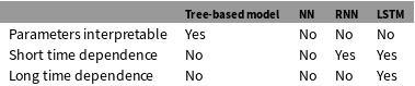
Summary of model differences.

Note: This is not intended to imply that models with these characteristics are “better” than models without them. NN stands for neural network. RNN stands for recurrent neural network, and LSTM stands for long short-term memory. Random forest is an example of a tree-based model.
The following equations show the prediction process for LSTM models for every time step  $t$. We give the dimensions of each term below. These dimensions depend on the dimensions of the predictors
 $D$ and the number of hidden units
 $H$, which is a hyperparameter.Footnote 10
 $x_{t}$ is a
 $D$-dimensional vector of predictors,
 $W$ is a
 $D\times H$ weight matrix,
 $U$, and
 $V$ are square,
 $H$-dimensional weight matrices, and
 $b$ is an
 $H$-dimensional bias vector with subscripts indicating the equation to which they correspond. The left-hand side of each equation is an
 $H$-dimensional prediction vector.
 $\unicode[STIX]{x1D70E}$ indicates the sigmoid function.Footnote 11 Keep in mind that the weights and biases are the trainable parameters or the parameters that take values that maximize accuracy based on the training data.
The first equation makes a prediction,  $g_{t}$, which can be conceptualized as a weighted sum of information the model takes in from the current word or word vector
 $x_{t}$ and the previous prediction of the final equation in the model
 $h_{t-1}$.
 $$\begin{eqnarray}g_{t}=\unicode[STIX]{x1D70E}(W_{g}x_{t}+U_{g}h_{t-1}+b_{g}).\end{eqnarray}$$
The sigmoid function ensures that the values of this initial prediction is between 0 and 1. These values are used in equation (7) to weigh how much information from the current word should be stored for use in making predictions based on future words. A 0 means no new information will be stored, and a 1 means all of the new information will be stored. The weights and bias vector in this equation allow the model to use information from the training set to decide which predictors are important for classification and, hence, should receive a higher weight. The term  $U_{i}h_{t-1}$ is the previous prediction
 $h_{t-1}$ weighted by the weight matrix
 $U_{i}$. In this way, the weight that the model puts on a predictor, in the case of text analysis a word or word vector, depends on how the model evaluated the previous predictor.
Next, the model evaluates how the information stored to model long time dependencies would change based on the current predictor and the previous prediction:
 $$\begin{eqnarray}\widetilde{C_{t}}=\text{tanh}(W_{c}x_{t}+U_{c}h_{t-1}+b_{c}).\end{eqnarray}$$
Next the model evaluates whether and how much information previously stored to evaluate long time dependencies should be erased or ‘forgotten’:
 $$\begin{eqnarray}f_{t}=\unicode[STIX]{x1D70E}(W_{f}x_{t}+U_{f}h_{t-1}+b_{f}).\end{eqnarray}$$
This value along with the prediction of equations (4) and (5) is used in the following equation that computes the new value of the information stored to evaluate long time dependencies. In this way, the model will decide to retain or discard information from the past based on the values of the weigh matrices  $W_{f}$ and
 $U_{f}$ as well as the bias
 $b_{f}$. Information for evaluating long time dependencies might be maintained, in part or whole, all the way to the end of a document, or it might be forgotten immediately depending on the values of these parameters.
Given the values of  $g_{t}$ (equation (4)),
 $\widetilde{C_{t}}$ (equation (5)), and
 $f_{t}$ (equation (6)), the model computes
 $C_{t}$, which is the new state of the information stored to evaluate long time dependencies:
 $$\begin{eqnarray}C_{t}=g_{t}\circ \widetilde{C_{t}}+f_{t}\circ C_{t-1}.^{12}\end{eqnarray}$$
The information used to evaluate long time dependencies,  $C_{t}$, is used to calculate the prediction below. Further, this information becomes
 $C_{t-1}$ in the next step. In this way, the model uses the information it has decided is useful to retain from previous steps in the calculation of the current prediction.
Given the new information about long time dependencies in the data,  $C_{t}$, the model computes
 $o_{t}$:
 $$\begin{eqnarray}o_{t}=\unicode[STIX]{x1D70E}(W_{o}x_{t}+U_{o}h_{t-1}+V_{o}C_{t}+b_{o}).\end{eqnarray}$$
This value places a weight on the final prediction. It serves a role similar to the prediction of equation (4), controlling the flow of information through the model.
Finally, the model calculates the final prediction as a function of the  $o_{t}$ from equation (8) and the value of information stored to evaluate long time dependencies,
 $C_{t}$, from equation (7):
 $$\begin{eqnarray}h_{t}=o_{t}\circ \text{tanh}(C_{t}).\end{eqnarray}$$
Neural network models are usually adapted to the problem they are applied to. To produce a single prediction between 0 and 1 for each text, our model ends in a logistic regression. See Appendix Section 5.5 for the full models we use. In practice, researchers often use bidirectional models that contain two LSTM models (Graves and Schmidhuber Reference Graves and Schmidhuber2005). One model reads the documents forward and the other reads the documents backwards. These models can pick up on different predictors and sometimes improve classification. The predictions of these models are then concatenated and sent to the final prediction equation, in our case, a logistic regression.
2.2.4 Training
The parameters begin at random values. To minimize misclassifications, neural network models iteratively adjust the parameters slightly and then check for improvement. These adjustments improve the fit if misclassifications decrease (for more information, see Appendix Section 5.2). How much the parameters are adjusted at each step is determined by the learning rate, which is a parameter set by the researcher (see Appendix Section 5.7.1 for advice on optimizing the hyperparameters of neural network models). An analogy can be drawn to the expectation–maximization algorithm that is familiar to political scientists from maximum likelihood estimation. Both algorithms initialize the parameters at random values and then repeatedly iterate using different estimates of the parameters until convergence.
3 Applications
3.1 Purpose
We use four applications to show LSTM models’ performance in different contexts. Because LSTM models differ in more than one way from alternative models, it is difficult to pinpoint exactly why the LSTM model performs better in any one task. Our purpose is instead to show the kinds of tasks where LSTM models perform well. The first three applications use a dataset of posts from the Chinese website Weibo, which is similar to Twitter. These posts are classified as either political or not political. The first application shows that in a large balanced dataset, ideal conditions for any classifier, LSTM models can outperform the alternatives. The second application shows that even as the size of this dataset is decreased by randomly sampling subsets of it, the LSTM model continues to perform well. The third shows that if we make this dataset unbalanced, the performance of the LSTM model decreases relative to competitors.
The fourth application compares an LSTM model with the SVM classifier deployed in another political science paper that classifies US newspaper articles based on whether they contain rape culture, specifically rape culture in the form of expressing empathy for the person accused of rape (Baum, Cohen, and Zhukov Reference Baum, Cohen and Zhukov2018). The point of this application is to show that LSTM models can sometimes improve classification accuracy under nonideal conditions where the classes are severely imbalanced. The purpose of this application is not to criticize original paper.
3.2 Classifying Weibo Posts
We evaluate how models perform classifying a subset of posts we collected from June 25, 2014 through June 15, 2015 that were hand-coded as either containing political content or not (see Appendix Section 5.1 for a full explanation of data collection, coding rules, and selection of the subset). The subset is balanced, containing 5,346 political posts and 5,345 nonpolitical posts. These posts are selected from a much larger dataset of posts. While the true prevalence of political posts is unknown, we estimate that less than 5% of the posts we originally collected are political.
We select several alternative document classifiers to compare our LSTM model against.Footnote 13 To get comparable accuracy scores, we focus only on models that assign an individual classification for each document. The first method we compare with is SVM, which is “the most widely used (and arguably the best) of the existing methods” (Hopkins and King Reference Hopkins and King2010, 239).Footnote 14 We also compare against both multinomial naive Bayes and Bernoulli naive Bayes, which are commonly used as baselines to compare classifiers against (D’Orazio et al. Reference D’Orazio, Landis, Palmer and Schrodt2014, 232–233). Finally, we compare against the extra-trees classifier, which is similar to the random forest classifier but is more computationally efficient and, in some cases, more accurate (Geurts, Ernst, and Wehenkel Reference Geurts, Ernst and Wehenkel2006). Extra-trees models are a useful comparison both because they are nonlinear and because they fit multiple randomly chosen models to the data, allowing them to capture complexity. This makes it a potential nonneural network model that researchers could use to classify documents that contain complex and nonlinear predictors.
We also combine these models, in some cases, with one of two different vectorizers in an attempt to improve their performance. The first is Word2vec (W2V). W2V is a type of word embedding that changes a corpus of words from unique identifiers that contain no information about how words relate to each other into a vector space where similar words are closer to each other.Footnote 15 The second is term frequency–inverse document frequency (TFIDF). TFIDF gives more weight to words that are rare in the corpus but common in a particular document and, hence, more likely to be distinguishing.Footnote 16
We do not compare against other variants of LSTM models because the largest study of LSTM model performance concluded that “The most commonly used LSTM architecture (vanilla LSTM) performs reasonably well on various datasets and using any of eight possible modifications does not significantly improve the LSTM performance” (Greff et al. Reference Greff, Srivastava, Koutník, Steunebrink and Schmidhuber2016). We do not compare against RNNs because LSTM models converge more quickly (Hochreiter Reference Hochreiter1998), which eliminates what one might expect to be the gain from using the simpler RNN model. Further, LSTM models are preferable over RNNs for “nontrivial tasks”(Hochreiter and Schmidhuber Reference Hochreiter, Schmidhuber, Mozer, Jordan and Petsche1997b, 478), where a trivial task is a problem that is quickly solvable by random search, making deep learning unnecessary in the first place.Footnote 17 Finally, we do not compare against MLP because, at least for classification tasks, MLP tends to offer no advantage over SVM (Osowski, Siwek, and Markiewicz Reference Osowski, Siwek and Markiewicz2004).Footnote 18
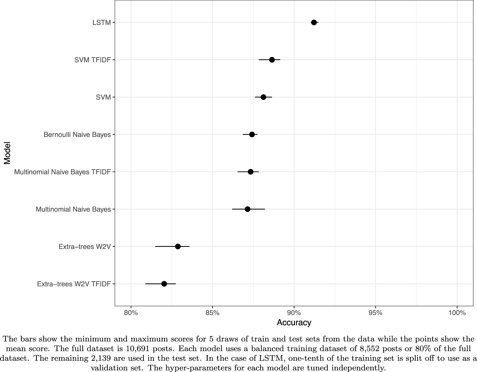
To express uncertainty around our accuracy scores, we draw five training and test sets from the data for each model and report the mean, minimum, and maximum test accuracy scores.Footnote 19 The train/test splits are stratified to ensure class balance. Traditional 95% confidence intervals cannot be used because supervised learning models like SVM and LSTM models are not founded on probability distributions (Hopkins and King Reference Hopkins and King2010, 239). The size of the training dataset for each model in each test is four-fifths of the full dataset or 8,552 posts. The remaining 2,139 posts are used as the test set.
For the LSTM models, one-tenth of the training set is split off to use as a validation set (see Section 1 on why validation is different with neural network models). Some readers might worry that our test is not a fair comparison because the LSTM model uses a validation set and the others do not. However, the LSTM model does not train on the validation set (James et al. Reference James, Witten, Hastie and Tibshirani2013, 178). We independently tune the hyperparameters of all the models using cross-validation. In this way, the competing models also get the advantage of using the full dataset to set their hyperparameters, so cross-validation to optimize the hyperparameters of competing models with tunable hyperparameters takes the place of a validation set for these models (James et al. Reference James, Witten, Hastie and Tibshirani2013, 178). If the LSTM model forgoes a validation set and is set to stop after 11 passes through the data, the results are substantially the same (see Appendix Section 5.6).
We preprocess the data in the same way for all the models. The classifiers are classifying posts in the original Chinese, which we segment using Jieba (Sun Reference Sun2015). For this application, we find that all the methods, not just LSTM, perform better when stop words, words that are so common that they are usually considered not meaningful for classification, and punctuation are not removed. This might be because social media posts are short, so the further removal of information decreases accuracy. For this reason, we do not remove stop words or punctuation. Chinese has no conjugation, so stemming (taking words down to their root so that, for an English example, “run,” “running,” and “ran” count as the same word) is not necessary.
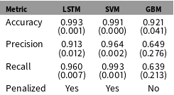
Classifying political vs. nonpolitical Weibo posts.

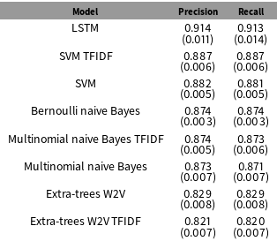
As shown in Figure 1, the mean accuracy of the LSTM model is over 2.53 percentage points higher than the next-best model (SVM TFIDF). A 2.5 percentage point increase may not sound like much, but this is actually quite a large difference. To put it into perspective, the next-best model’s mean accuracy is only about 1.2 percentage points higher than the best performing of the naive Bayes models. This means the improvement from switching from SVM TFIDF to an LSTM model for this dataset is more than double the improvement from switching to SVM TFIDF from Bernoulli naive Bayes, which is typically used as a baseline model. The LSTM model consistently performs better across every train and test set drawn. The worst performing LSTM test is still over 2 percentage points more accurate than that of the best performing test for SVM TFIDF. Table 2 shows how these models perform on precision (identifying nonpolitical posts as not political) and recall (identifying political posts as political). The LSTM model outperforms the other models on both metrics.
Precision and recall.

Note: The mean scores from the five train and test set draws are shown with standard errors in parentheses. Precision measures whether the models identify nonpolitical posts correctly, and recall measures whether the model identifies political posts correctly.
Here are two examples of posts from the data where word context is important for correct classification, and SVM TFIDF incorrectly classifies the post while LSTM classifies it correctly. The first post appears to be about friendship, but in the context of the Asia-Pacific Economic Cooperation (APEC) conference leaving Beijing, it is actually pointing out that the government manipulates pollution levels to make China look good to international audiences but allows pollution to return once the world’s attention is elsewhere.
‘APEC’ has gone, and our old friends [air pollution] have returned to us. [Our old friends] never abandon us or give us up. Such friends are absolutely loyal. ‘APEC’  ,
 ,


The second post is actually non-political. However, because “climb onto the wall” ( ) often means bypassing the Great Firewall, SVM TFIDF classifies it as political, even though the phase does not have that meaning in this context.
A while ago, I suddenly wanted to go to the Internet cafe to go online. I went to the school wall and climbed onto the wall. Surprisingly, just when I climbed up, a school security guard came and called to me in the distance. I said, “Is it possible to come in to the school and find someone?” Security: “No! Get out right away!” Then I got out… ,
 ,
 ,
 ,
 : “
 ”

 : “
 ”

3.2.1 Computation Time
Another important performance metric is speed. LSTM models do take longer than traditional models to train. In this application, our LSTM model takes 2 minutes and 51 seconds to train and test for one draw from the data. This is when running the model on a desktop with an NVIDIA GeForce GTX 760 GPU and 7 gigabytes of RAM. This is a relatively old GPU that has exactly the minimum computing power required to run NVIDIA’s Deep Neural Network library (see Appendix Section 5.7.4). If the model is instead run on the Intel Core i5 CPU of one of the authors’ laptops with 3 gigabytes of RAM, it takes 5 minutes and 40 seconds.Footnote 20 In comparison, SVM takes about 20 seconds to train and test for one draw from the data on the laptop. This time difference has the biggest impact when tuning hyperparameters because the researcher will need to run the model repeatedly with different parameters. The good news is that researchers can automate this process and perform other tasks while tuning takes place. We have provided scripts to facilitate this.Footnote 21
3.3 Classifying with Small Samples
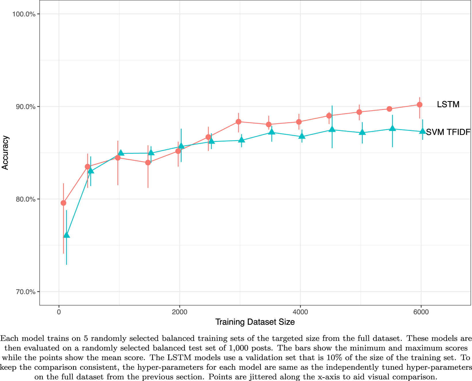
In this section, we test how the two models that performed best on the full dataset, the LSTM model and the SVM TFIDF model, perform on random, balanced subsamples of the data. The purpose of this is to examine how LSTM model performance changes as the size of the training set shrinks. Good performance with relatively small training samples is important for political science uses because it is expensive and time consuming to code large training datasets. We start with a randomly selected balanced training dataset of 6,000 posts taken from the original data. We then decrease the size of the training dataset by intervals of 500. We also include a test where the training dataset only contains 100 posts. The models are evaluated on a randomly selected balanced test set of 1,000 posts. We repeat this process five times for each training dataset size to get minimum, maximum, and mean scores. The LSTM model uses a validation set of one-tenth the size of the training set.
Accuracy with changing sample sizes.

As shown in Figure 2, the LSTM model continues to achieve higher mean scores than the SVM TFIDF model until the size of the training dataset drops below 2,500 posts. While collecting large training sets can be costly,Footnote 22 LSTM will generally provide greater returns to researchers willing to pay this cost because they hit the point of diminishing returns from added data more slowly.
3.4 Classifying with Unbalanced Data
Political scientists often work with unbalanced data, meaning data where one category is more common than another. To compare performance with unbalanced data, we add additional nonpolitical posts to create a dataset with 45,000 nonpolitical posts and 5,346 (about 10% of the total) political posts.Footnote 23 Unbalanced sets like this are difficult for models to train on because models will tend to classify every post as not political and get 90% accuracy.
One way to deal with this challenge is to penalize incorrect classifications of the less common category more heavily. Another way to deal with class unbalance is to use gradient boosting. GBM are a tree-based model that uses gradient boosting. Interested readers should see Montgomery and Olivella (Reference Montgomery and Olivella2018). Because GBM train sequentially, they are able to devote more trees at each step to the class that they classify incorrectly (Weiss Reference Weiss2004). Other techniques for dealing with unbalanced data include undersampling the more common class and synthetic minority oversampling (SMOTE). These methods are beyond the scope of this paper, but interested readers should see Liu, Wu, and Zhou (Reference Liu, Wu and Zhou2009) on undersampling and Chawla et al. (Reference Chawla, Bowyer, Hall and Kegelmeyer2002) and Fernández et al. (Reference Fernández, Garcia, Herrera and Chawla2018) on SMOTE. Here we compare an LSTM model and an SVM model, which penalize misclassification in inverse proportional to the frequency of categories in the data, with GBM.
As shown in Table 3, both SVM and LSTM perform well with accuracy of over 99% and precision and recall over 90%. However, SVM notably outperforms LSTM on precision and recall. As the application in Section 3.5 reveals, SVM does not always outperform LSTM on unbalanced datasets, but it is reasonable to expect that unbalanced data will increase the performance of SVM in the comparison with LSTM, holding the task constant. This is because neural network models perform best on tasks with a “high signal-to-noise ratio” (Friedman, Hastie, and Tibshirani Reference Friedman, Hastie and Tibshirani2001, 408). It is tempting to dismiss GBM’s performance as poor, but it is classifying over 90% of posts correctly with balanced accuracy (meaning precision and recall are approximately equal). This improves on models not adjusted to handle unbalanced data, which would achieve similar levels of accuracy but with near 0 recall.
Unbalanced Weibo results.

Note: The mean scores from five train and test set draws are shown with standard errors in parentheses. Precision measures whether the models identify nonpolitical posts correctly, and recall measures whether the model identifies political posts correctly.
3.5 Classifying US Newspaper Articles
Baum, Cohen, and Zhukov (Reference Baum, Cohen and Zhukov2018) train an SVM TFIDF classifier to classify US newspaper articles on various indicators of rape culture. We choose the indicator, empathy for the accused, where their classifier performs the least well and examine whether an LSTM model can offer improvement. We suspect that contextual information may improve classification of this variable because it is important to know who the article is expressing empathy for, the victim or the accused.
We follow the practices of the original authors by removing stop words, punctuation, and stemming.Footnote 24 We also follow the original authors in using the “pooled” dataset that contains multiple entries for articles where their human coders disagree.Footnote 25 This dataset contains 21,911 human-labeled articles.
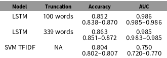
For all of our LSTM models on Weibo posts, we preserved the length of every post by padding them to the length of the longest post. While this is possible to do for longer documents, it is impractical in terms of computation time and resource demands (the longest article is over 3,000 words). For the LSTM model, we first try truncating the post to the first 100 words to see if performance is satisfactory. To address the possible concern that this truncation may somehow bias the comparison in favor of LSTM, we show that the results are essentially unchanged if truncation is extended to the mean length of newspaper articles in the dataset (339 words). The results for SVM TFIDF we report come directly from Baum, Cohen, and Zhukov (Reference Baum, Cohen and Zhukov2018) where SVM TFIDF was allowed to train on the entire length of the articles.
Baum, Cohen, and Zhukov (Reference Baum, Cohen and Zhukov2018) do not report precision and recall, but they report out-of-sample accuracy as well as area under the receiver operating characteristic (ROC) curve, so we compare these two metrics.Footnote 26 Baum, Cohen, and Zhukov (Reference Baum, Cohen and Zhukov2018) report results both for 10-fold cross-validation as well as 10 trials of random re-sampling with a 75/25 train/test split. We compare against their classifier’s 10-fold cross-validation results, which are its best. However, for our own model, we use random re-sampling with a 75/25 train/test split, which makes the training set of our model smaller than that of the model we are comparing against. We do not use a validation set in this application.
The categories are unbalanced. Only about 1 in every 6.89 articles expresses empathy for the accused. For this reason, it is important to focus on area under the curve (AUC) in addition to accuracy because a model could predict that every article is a 0 (contains no empathy for the accused) and achieve out-of-sample accuracy of about 88%. To prevent our model from doing this, we penalize misclassification in inverse proportion to the observed class frequencies.Footnote 27
Comparing newspaper classifiers.

Note: The mean score from the train and test set draws are shown with the range between the best and worst scores below.
The results in Table 4 show that the LSTM model outperforms the SVM TFIDF model from the original paper by about 5 percentage points in accuracy (6 points when truncation is extended to 339 words). The model improves the AUC by approximately 23 percentage points. This indicates that many more of the true positives are correctly classified as containing empathy for the accused by the LSTM model. We speculate that the size of the improvement is larger here than in the Weibo post application because of the greater importance of context for understanding whether an article is expressing empathy and, if so, for whom the newspaper article is empathizing. Parsing empathy may even require going a sentence or two back in the text, making it a good case for applying an LSTM model. LSTM models are able to parse features like this because they extract features the model has learned are useful for interpreting words or word vectors that may occur later in documents (see Section 2.2). This application also shows that, at least for some cases of unbalanced data, LSTM can outperform SVM TFIDF.
4 Conclusion
LSTM models perform best relative to traditional models in applications with large training sets where words within documents have complex context-dependent relationships. LSTM models perform less well relative to traditional models as the amount of unbalance among categories in the data increases. LSTM models are adaptable to a wide variety of tasks and can classify texts on any basis the researcher desires provided they have adequate training data. Our examples are binary, mutually exclusive tasks for the sake of simplicity, but LSTM models can classify texts into more than two categories as well as in situations where categories are not mutually exclusive. Further, LSTM models can classify texts regardless of their language. We hope that the guidance we provide about the use of these models along with our code templates facilitates the use of these models in future political science applications.
Future work should continue to explore the relatively untapped political science potential of LSTM models. For example, LSTM models have applications for time-series forecasting that may prove useful for political scientists working with event data (Maknickiene and Maknickas Reference Maknickiene and Maknickas2012). This is because the characteristics that allow LSTM models to learn long time dependencies, such as the relationship between the words at the beginning of a document and the words at the end of a document, can be applied to time-series data where predictors from the past have systematic yet complex relationships with events in the future.
Acknowledgements
The authors contributed equally. We thank Ling, Qingwei, Tami, and Wenchang for their ever-awesome research assistance. Thanks to Sarah Bouchat, Devin Judge-Lord, Melanie Manion, Eleanor Powell, Molly Roberts, Alex Tahk, Samantha Vortherms, Zach Warner, Jessica Weeks, and Chagai Weiss for helpful comments on drafts of this paper.
Supplementary materials
For supplementary materials accompanying this paper, please visit https://doi.org/10.1017/pan.2019.46.