





1. Introduction
Since turbulent motions significantly enhance skin friction drag compared with the corresponding laminar flow, skin friction drag reduction is of great importance for energy saving. Among numerous flow control methods for friction drag reduction (Kim Reference Kim2003; Kasagi, Suzuki & Fukagata Reference Kasagi, Suzuki and Fukagata2009; Ricco, Skote & Leschziner Reference Ricco, Skote and Leschziner2021; Fukagata, Iwamoto & Hasegawa Reference Fukagata, Iwamoto and Hasegawa2024), the opposition control proposed by Choi, Moin & Kim (Reference Choi, Moin and Kim1994) is the simplest feedback control method. In this control method, a detection plane parallel to the wall is placed in the flow field, and the wall-normal velocity opposite to that detected on the detection plane is imposed on the wall. Choi et al. (Reference Choi, Moin and Kim1994) and Hammond, Bewley & Moin (Reference Hammond, Bewley and Moin1998) achieved a friction drag reduction of about  $25\,\%$ in a low-Reynolds-number turbulent channel flow by direct numerical simulation (DNS). According to Hammond et al. (Reference Hammond, Bewley and Moin1998), the formation of the virtual wall in the fluid halfway between the physical wall and the detection plane, in which the wall-normal velocity fluctuations are approximately zero, results in the suppression of the momentum transport in the wall-normal direction, leading to a large drag-reduction effect. However, the details of the drag-reduction mechanism such as the effects of the virtual wall and turbulent energy transport in the opposition-controlled flow are still under investigation.
Nonlinear dynamical systems have provided a firm platform for dealing with diverse dynamical states: intermittency and deterministic chaos appearing in various aperiodic flow convections related to wall turbulence (Aubry et al. Reference Aubry, Holmes, Lumley and Stone1988; Sanghi & Aubry Reference Sanghi and Aubry1993; Holmes, Lumley & Berkooz Reference Holmes, Lumley and Berkooz1996; Waleffe Reference Waleffe1997; Eckhardt & Mersmann Reference Eckhardt and Mersmann1999; Moehlis, Faisst & Eckhardt Reference Moehlis, Faisst and Eckhardt2004; Cavalieri Reference Cavalieri2021; Cavalieri & Nogueira Reference Cavalieri and Nogueira2022; Cavalieri, Rempel & Nogueira Reference Cavalieri, Rempel and Nogueira2022). The strange attractor in dynamical systems exhibits an impressive geometrical pattern structure in a phase space. In the context of dynamical systems and information theory, the pattern of trajectories in a phase space can be linked to a finite string of symbolics (Amigó Reference Amigó2010). Ordinal patterns, which are defined by the rank order relations among continuous points of trajectories, are the Markov partition-based symbolic string representations that enable the unravelling of the structure of a phase space (Amigó Reference Amigó2010). The importance of ordinal patterns was first shown by Bandt & Pompe (Reference Bandt and Pompe2002) in their seminal and foundational works on permutation entropy (PE). Their works have paved a new way to the construction of a system for contemporary ordinal pattern-based analysis in the fields of mathematical science and related nonlinear physics. There are various useful methods that are of fundamental importance for evaluating the dynamical complexity, involving the PE (Bandt & Pompe Reference Bandt and Pompe2002), the forbidden pattern number (Kulp & Zunino Reference Kulp and Zunino2014; McCullough et al. Reference McCullough, Sakellariou, Stemler and Small2016), symbolic recurrence plots (Marwan et al. Reference Marwan, Romano, Thiel and Kurths2007; Caballero-Pintado, Matilla-Garcia & Marin Reference Caballero-Pintado, Matilla-Garcia and Marin2018) and the complexity–entropy causality plane (CECP) (Rosso et al. Reference Rosso, Larrondo, Martin, Plastino and Fuentes2007). The PE is the information entropy of the symbols representing the rank-order patterns encoded from a time series and is the most well-used metric capable of quantifying the randomness of dynamic behaviour. The CECP is a two-dimensional plane consisting of the PE and Jensen–Shannon complexity to quantify the complexity of dynamic behaviour. The multiscale CECP (Zunino, Soriano & Rosso Reference Zunino, Soriano and Rosso2012) considering the embedding delay time in a phase space has shown to be an effective method for distinguishing between chaos and the stochastic process. These methods have enabled appropriate characterisation encompassing the understanding of the dynamical states appearing in a broad range of fluid phenomena: laminar–turbulent transition in a boundary layer flow (Li & Zuntao Reference Li and Zuntao2014; Zhang et al. Reference Zhang, Liu, Guo and Wang2017b), laboratory-scale plasmas and solar wind (Weck et al. Reference Weck, Schaffner, Brown and Wicks2015), falling liquid films (Gotoda, Pradas & Kalliadasis Reference Gotoda, Pradas and Kalliadasis2017b), a turbulent coaxial jet (Kobayashi et al. Reference Kobayashi, Gotoda, Kandani, Ohmichi and Matsuyama2019) and a turbulent channel flow (Mamori et al. Reference Mamori, Nabae, Fukuda and Gotoda2023). One of the present authors (Hayashi, Gotoda & Gentili Reference Hayashi, Gotoda and Gentili2016; Gotoda, Kobayashi & Hayashi Reference Gotoda, Kobayashi and Hayashi2017a; Takagi et al. Reference Takagi, Gotoda, Tokuda and Miyano2017; Murayama et al. Reference Murayama, Kinugawa, Tokuda and Gotoda2018; Nomi et al. Reference Nomi, Gotoda, Kandani and Almarcha2021) has highlighted the applicability of ordinal pattern-based analysis to chemically reacting flow systems.
The substantial progress of network science originating from graph theory has led to diverse complex networks: the visibility graph (Lacasa et al. Reference Lacasa, Luque, Ballesteros, Luque and Nuno2008), a correlation network (Gao & Jin Reference Gao and Jin2009), the cycle network (Zhang & Small Reference Zhang and Small2006), the recurrence network (Marwan et al. Reference Marwan, Romano, Thiel and Kurths2007) and the turbulence network (Taira, Nair & Brunton Reference Taira, Nair and Brunton2016). The complex-network approach has established a promising platform of analytical methods to expand our understanding of spatiotemporal dynamics in various turbulent flows (Gao & Jin Reference Gao and Jin2009; Lozano-Durán & Jiménez Reference Lozano-Durán and Jiménez2014; Taira et al. Reference Taira, Nair and Brunton2016; Gotoda et al. Reference Gotoda, Pradas and Kalliadasis2017b; Iacobello et al. Reference Iacobello, Scarsoglio, Kuerten and Ridolfi2018; Kobayashi et al. Reference Kobayashi, Gotoda, Kandani, Ohmichi and Matsuyama2019; Bae & Lee Reference Bae and Lee2021; Chowdhuri, Iacobello & Banerjee Reference Chowdhuri, Iacobello and Banerjee2021; Iacobello, Ridolfi & Scarsoglio Reference Iacobello, Ridolfi and Scarsoglio2021; De et al. Reference De, Gupta, Unni, Ravindran, Kasthuri, Marwan, Kurths and Sujith2023; Mamori et al. Reference Mamori, Nabae, Fukuda and Gotoda2023). Along the line of the concept of symbolic dynamics, Small and co-workers (Small Reference Small2013; McCullough et al. Reference McCullough, Small, Stemler and Iu2015) proposed the ordinal partition transition network (OPTN) as a specific type of transition network. Mamori et al. (Reference Mamori, Nabae, Fukuda and Gotoda2023) have recently shown that the univariate OPTN entropy is useful for assessing the randomness of the streamwise velocity in a turbulent channel flow. They also clarified the formation of a low-dimensional (high-dimensional) chaotic state of the streamwise velocity fluctuations at a viscous sublayer (logarithmic layer). This recent study by Mamori et al. (Reference Mamori, Nabae, Fukuda and Gotoda2023) has importantly brought about a foothold for the interdisciplinary fusion between symbolic and turbulent dynamics. One of our primary interests and motivations in this study is to extend our understanding of the drag-reduction mechanism on controlled turbulent channel flow by clarifying the physical link between the symbolic dynamics-based complexity metrics and the spatiotemporal structure of uncontrolled/controlled turbulent channel flow. This challenging subject still remains unexplored over a long period of wall-turbulent flow research. In fact, notwithstanding the many uncontrolled/controlled wall-turbulent flow studies (Kim Reference Kim2003; Kasagi et al. Reference Kasagi, Suzuki and Fukagata2009; Ricco et al. Reference Ricco, Skote and Leschziner2021; Fukagata et al. Reference Fukagata, Iwamoto and Hasegawa2024) using DNS, the details of the drag-reduction mechanism of the opposition-controlled flow have not been investigated even under a low-Reynolds-number condition from the viewpoint of the symbolic dynamics approach.
On the basis of the above background, the main objective of this study is to investigate the drag-reduction mechanism of an opposition-controlled turbulent channel flow by ordinal pattern-based analysis, with a particular focus on the effect of the virtual wall. In this study, we consider the multivariate OPTN (Zhang et al. Reference Zhang, Zhou, Tang, Guo, Small and Zou2017a), multiscale CECP, and spatial permutation entropy (SPE) (Zunino & Ribeiro Reference Zunino and Ribeiro2016). The rest of the paper is organised into four sections. In §§ 2 and 3, we explain the basic framework of DNS and ordinal pattern-based analysis, respectively. In § 4, we present the drag-reduction mechanism, showing the applicability of ordinal pattern based-analysis to the appropriate control of a turbulent channel flow. We provide a summary in § 5.
2. Direct numerical simulation
The governing equations are the incompressible continuity and Navier–Stokes equations, i.e.
 $$\begin{gather} \frac{\partial u_i}{\partial x_i} = 0, \end{gather}$$
 $$\begin{gather}\frac{\partial u_i}{\partial t} =-\frac{\partial (u_iu_j)}{\partial x_j} - \frac{\partial p}{\partial x_i} + \frac{1}{ Re_\tau }\frac{\partial^2 u_i}{\partial x_j \partial x_j}-\frac{{\rm d}P}{{\rm d}\kern0.06em x_1}\delta_{i1}, \end{gather}$$
where  $u_i\ ( i=1,2,3)$ and
 $p$ denote the velocity components and pressure, respectively. Moreover,
 $1$,
 $2$ and
 $3$ denote the streamwise, wall-normal and spanwise directions, respectively. All variables are made dimensionless by the friction velocity
 $u^{\ast }_{\tau }$, channel half-width
 $\delta ^{\ast }$ and fluid density
 $\rho ^{\ast }$, where the superscript
 $\ast$ denotes dimensional quantities. We perform all simulations under a constant pressure gradient (CPG) condition at
 $Re_\tau = u_{\tau }^{\ast } \delta ^{\ast }/\nu ^{\ast } = 180$ and
 $590$, where
 $\nu ^\ast$ is the kinematic viscosity. The computational conditions in the present DNS are summarised in table 1, where
 $L_i$,
 $N_i$ and
 $\Delta x_i$ denote the computational domain, the number of grid points and the grid spacing, respectively, in the
 $i$th direction, and
 $\Delta t$ is the time resolution of DNS. Note that the superscript + represents wall units non-dimensionalised by the friction velocity and kinematic viscosity.
Computational conditions in the present DNS.

The DNS code used in this study is based on that developed by Fukagata, Kasagi & Koumoutsakos (Reference Fukagata, Kasagi and Koumoutsakos2006) and extended by Nabae & Fukagata (Reference Nabae and Fukagata2024). The governing equations are spatially discretised using the energy-conserving fourth-order finite-difference scheme (Morinishi et al. Reference Morinishi, Lund, Vasilyev and Moin1998) in the streamwise and spanwise directions and the second-order finite-difference scheme in the wall-normal direction. The time integration is conducted using the low-storage third-order Runge–Kutta/Crank–Nicolson scheme (Spalart, Moser & Rogers Reference Spalart, Moser and Rogers1991) with the higher-order simplified marker and cell (SMAC)-like velocity–pressure coupling scheme (Dukowicz & Dvinsky Reference Dukowicz and Dvinsky1992). The pressure Poisson equation is solved by the fast Fourier transformation in the streamwise and spanwise directions and the tridiagonal matrix algorithm in the wall-normal direction.
We apply the periodic boundary condition in the streamwise and spanwise directions. The boundary conditions for the streamwise and spanwise velocities on the walls are  $u = 0$ and
 $w = 0$, respectively. In addition, the boundary conditions for the wall-normal velocity on the walls in the uncontrolled and controlled cases are
 $v = 0$ and
 \begin{equation} \left.\begin{array}{c@{}} v (\kern0.09em y=0 ) =-v (\kern0.09em y=y_d ) \quad \text{(lower wall)}, \\ v (\kern0.09em y=2 ) =-v (\kern0.09em y=2-y_d ) \quad \text{(upper wall)}, \end{array}\right\} \end{equation}
respectively, where  $y_d$ denotes the location of the detection plane shown in figure 1. In this study, we set five different detection planes, i.e.
 $y_d^+ \approx 5$, 7.5, 10, 15 and
 $20$.
Schematic of opposition control.

The drag-reduction rate  $R_D$ is defined as
 \begin{equation} R_D = 1-\frac{ C_f }{ C_{f0} }, \end{equation}
where  $C_f$ and
 $C_{f0}$ are the drag coefficients in the controlled and uncontrolled cases, respectively. These drag coefficients are calculated as
 $C_f = 1/{U_b^{+}}^2$ and
 $C_{f0}=1/{U_{b,NC}^{+}}^2$, respectively. Here,
 $U_{b,NC}^+$ is the bulk-mean velocity in the uncontrolled case. Similarly to Nabae, Kawai & Fukagata (Reference Nabae, Kawai and Fukagata2020),
 $U_{b,NC}^+$ is calculated using the approximation formula proposed by Nabae et al. (Reference Nabae, Kawai and Fukagata2020) regarding the relationship between the bulk Reynolds number and the bulk-mean velocity in the uncontrolled case, i.e.
 \begin{equation} U^+_{b,NC} = 5.1904 \log Re_b - 3.6741, \end{equation}
where the resultant bulk Reynolds number is calculated as  $Re_b = 2U_b^+ Re_\tau$. Note that
 $U_b$ can be calculated as
 \begin{equation} U_b = \frac{1}{2} \int_0^2 U(y) \,{{\rm d} y}, \end{equation}
where  $U(y)$ is the streamwise velocity averaged in the streamwise and spanwise directions and time.
Figure 2 shows the drag-reduction rates at different  $y_d^+$ values in all cases. Similarly to Hammond et al. (Reference Hammond, Bewley and Moin1998), we can obtain the maximum drag-reduction rate of
 $R_D \approx 25\,\%$ at
 $y_d^+ \approx 15$. Thus, the computational conditions in the present DNS can be considered sufficient for simulating a low-Reynolds-number turbulent channel flow.
Drag-reduction rates at different  $y_d^+$ values in all cases.

3. Analytical methods
3.1. Ordinal partition transition network
Zhang et al. (Reference Zhang, Zhou, Tang, Guo, Small and Zou2017a) proposed the multivariate OPTN considering the combination of permutation patterns extracted from  $n$ multivariate time series. Similarly to their study, we construct the multivariate OPTN to evaluate the correlations between temporal evolutions of the streamwise and wall-normal velocity fluctuations
 $u^{\prime }$ and
 $v^{\prime }$, respectively. Figure 3 shows the schematic of construction of the multivariate OPTN. First, we transform the elements of
 $\boldsymbol {u}$ (=
 $\{ u^{\prime }(t_i), u^{\prime }(t_i+\tau _t),\ldots, u^{\prime }(t_i+\tau _t(d_t-1) \} )$ and
 $\boldsymbol {v}$ (
 $= \{ v^{\prime }(t_i), v^{\prime }(t_i+\tau _t),\ldots, v^{\prime }(t_i+\tau _t(d_t-1) \} )$ into rank-order patterns (permutation patterns) based on the magnitude of these elements, where
 $d_t$ is the embedding dimension (the rank-order pattern length) and
 $\tau _t$ is the delay time in a phase space (figure 3 represents the case of
 $d_t = 2$ and
 $\tau _t = \Delta t$). A combination of permutation patterns
 $\varPi ( = \{ \varPi _1,\varPi _2,\ldots,\varPi _{d_t!^{2n}} \} )$ corresponds to nodes in the network, and the link between two nodes is expressed by the transition probability from
 $\varPi _i$ to
 $\varPi _j$, i.e.
 $p_t(\varPi _i \to \varPi _j)$. We calculate the multivariate OPTN entropy, i.e.
 \begin{equation} H_t =- \frac{ \displaystyle\sum^{d_t!^n}_{i=1}\sum^{d_t!^n}_{j=1} p_t(\varPi_i \to \varPi_j) \ln{ p_t(\varPi_i \to \varPi_j) } }{ \ln{ (d_t!)^{2n} } }, \end{equation}
where  $0\leq H_{t}\leq 1$. The multivariate OPTN entropy
 $H_t$ can quantify the degree of randomness in the simultaneous dynamic behaviour of the two different time evolutions of
 $u^\prime$ and
 $v^\prime$. We construct the multivariate OPTN from the temporal evolutions of
 $u^{\prime }$ and
 $v^{\prime }$ at the centre of each
 $x$–
 $z$ plane, i.e.
 $x = L_x/2$,
 $0 \leq y \leq 1$ and
 $z = L_z/2$. The length of these time series is
 $t^+ \approx 10\,000$. To determine a suitable value of
 $d_t$, Nomi et al. (Reference Nomi, Gotoda, Kandani and Almarcha2021) proposed a method considering missing permutation patterns of a time series (Amigó, Zambrano & Sanjuán Reference Amigó, Zambrano and Sanjuán2007). According to their study, missing permutation patterns appear at
 $d_t \geq 4$ for Gaussian noise. We also observe missing permutation patterns for fractional Brownian motion with the Hurst exponent of
 $1/3$ exhibiting Kolmogorov's five-third scaling law in the power spectrum (Meerschaert et al. Reference Meerschaert, Sabzikar, Phanikumar and Zeleke2014). These results mean that the values at
 $d_t \geq 4$ are not suitable for constructing the OPTN. Thus, we set
 $d_t = 3$. In this study, we define a local link strength between
 $\varPi _i$ and
 $\varPi _j$ as
 $s_{\varPi _i \rightarrow \varPi _j} (= p_t(\varPi _i \rightarrow \varPi _j)).$ Note that
 $s_{\varPi _i \rightarrow \varPi _j}$ represents the transition degree between instantaneous fluid patterns.
Schematic of construction of the multivariate OPTN when  $d_t = 2$ and
 $\tau _t = \Delta t$.

To determine a suitable value of  $\tau _t$, we investigate the dependence of
 $\tau _t$ on
 $H_t$ in the uncontrolled case. Figure 4 shows the variation in
 $H_t$ as a function of
 $y^+$ at six different
 $\tau _t^+$ values. In the cases of
 $\tau _t^+ = \Delta t^+$,
 $150 \Delta t^+$ and
 $300 \Delta t^+$, the dependence of
 $H_t$ on
 $y^+$ is relatively small, whereas in the other cases, especially
 $\tau _t^+ = 30 \Delta t^+$,
 $H_t$ notably changes as a function of
 $y^+$. According to Mamori et al. (Reference Mamori, Nabae, Fukuda and Gotoda2023), the low-dimensional (high-dimensional) chaotic state of streamwise velocity fluctuations emerges at the viscous sublayer (logarithmic layer). This dynamical change from the low- to high-dimensional chaotic state increases the degree of randomness of streamwise velocity fluctuations with
 $y^+$. This trend can be clearly observed in the case of
 $\tau _t^+ = 30 \Delta t^+ = 1.08$, which is the same as the value of
 $\tau _t$ mainly utilised by Mamori et al. (Reference Mamori, Nabae, Fukuda and Gotoda2023). Therefore, in this study, we estimate the local link strength in the multivariate OPTN constructed at
 $\tau _t^+ = 30\Delta t^+ =1.08$.
Variation in the multivariate OPTN entropy  $H_t$ as a function of
 $y^+$ at six different
 $\tau ^+_t$ values.

3.2. Complexity–entropy causality plane
The CECP (Zunino et al. Reference Zunino, Soriano and Rosso2012) considering a time-dependent approach, namely, the multiscale CECP, is useful for inferring the dynamical state in nonlinear systems. The CECP consists of the Jensen–Shannon complexity  $C_{JS}$ and PE
 $H_p$, i.e.
 $$\begin{gather} C_{JS}[\boldsymbol{P_p}] = Q_J[ \boldsymbol{P_p},\boldsymbol{P_e} ] H_p[\boldsymbol{P_p}], \end{gather}$$
 $$\begin{gather}H_p[\boldsymbol{P_p}] =-\frac{ \displaystyle\sum^{d_C!}_{j=1}p_p({\rm \pi}_j)\ln{p_p({\rm \pi}_j)} }{ \ln{d_C!} }, \end{gather}$$
where  $Q_J$ is the disequilibrium, i.e.
 $$\begin{gather} Q_J [\boldsymbol{P_p},\boldsymbol{P_e}] = \frac{ H_p [(\boldsymbol{P_p}+\boldsymbol{P_e})/2] - H_p[\boldsymbol{P_p}]/2 - H_p[\boldsymbol{P_e}]/2 } {Q_{J,{max}} }, \end{gather}$$
 $$\begin{gather}Q_{J,{max}} =-\frac{1}{2} \left \{ \frac{d_C! + 1}{d_C!} \ln (d_C! + 1) - 2\ln (2 d_C!) + \ln d_C! \right \}. \end{gather}$$
Here,  $\boldsymbol {P_p} = \{\,p_p({\rm \pi} _j) \,|\, j=1,2,\ldots,d_C!) \}$ is the existing probability distribution of the permutation patterns
 ${\rm \pi} _j$ in the time series of
 $u^{\prime }$ and
 $\boldsymbol {P_e} = \{ 1/d_C!,1/d_C!,\ldots,1/d_C! \}$ is the uniform probability distribution, where
 $d_C$ is the embedding dimension. Here,
 $H_p$ represents the degree of randomness in the time evolution of
 $u^\prime$ and
 $Q_J$ represents the disequilibrium in the probability distribution of the permutation patterns obtained from the time evolution of
 $u^\prime$. In addition,
 $C_{JS}$ is defined as the product of
 $H_p$ and
 $Q_J$, which corresponds to the statistical complexity in the time evolution of
 $u^\prime$.
The dynamical state can be inferred from the shape of the trajectory on the CECP with the increasing delay time  $\tau _C$ in
 $d_C$-dimensional phase space. If the dynamic behaviour exhibits deterministic chaos, a parabolic trajectory is drawn on the CECP. If the dynamic behaviour is strongly dominated by a stochastic process, no parabolic trajectory is drawn on the CECP and
 $(H_p,C_{JS})$ rapidly approaches
 $(1,0)$ with increasing
 $\tau _C$. Zunino et al. (Reference Zunino, Soriano and Rosso2012) reported that
 $\tau _C$ at which
 $C_{JS}$ takes a local maximum value corresponds to the minimal sampling rate required to capture all the information related to nonlinear correlations of the underlying chaotic dynamics. In this study,
 $d_C = 5$ and
 $0.036 \leq \tau _C^+ \leq 10.8$.
3.3. Spatial permutation entropy
The SPE (Zunino & Ribeiro Reference Zunino and Ribeiro2016) enables us to quantitatively evaluate the degree of spatial randomness. Figure 5 shows a schematic of the transformation from  $u^\prime$ to spatial permutation
 ${\rm \pi} _j$. For the estimation of the SPE, we first construct permutation patterns in the extraction range of
 $d_x d_z$, i.e. motifs, where
 $d_x$ and
 $d_z$ represent the numbers of extracted points in the streamwise and spanwise directions, respectively (figure 5 represents the case of
 $d_x = d_z = 2$). Subsequently, all motifs in the entire spatial field are classified into each permutation pattern to generate the existing probability distribution
 $\boldsymbol {P_{sp}}$. We calculate the SPE
 $H_{sp}$, i.e.
 \begin{equation} H_{sp}[\boldsymbol{P_{sp}}] =-\frac{ \displaystyle\sum^{( d_x d_z )!}_{j=1} p_{sp}({\rm \pi}_j) \ln{p_{sp}({\rm \pi}_j)} }{ \ln{( d_x d_z )!} }, \end{equation}
where  $0\leq H_{sp}\leq 1$. Note that
 $H_{sp}$ represents the degree of randomness in the instantaneous field of
 $u^\prime$. Here,
 $\boldsymbol {P_{sp}} = \{\,p_{sp}({\rm \pi} _j) | \,j=1,2,\ldots,( d_x d_z )! \}$ is the existing probability distribution of the permutation patterns
 ${\rm \pi} _j$ in the spatial field data of
 $u^{\prime }$ in each
 $x$–
 $z$ plane. In this study,
 $(d_x,d_z) = (3,2)$.
Schematic of transformation from  $u^\prime$ to spatial permutation
 ${\rm \pi} _j$ when
 $d_x = d_z = 2$.

4. Results and discussion
Figure 6 shows the weighted Reynolds shear stress (RSS) (Fukagata, Iwamoto & Kasagi Reference Fukagata, Iwamoto and Kasagi2002), i.e.  $2( 1-y^+/Re_\tau ) ( -\overline {u^\prime v^\prime } )$, in the uncontrolled and controlled cases. In the uncontrolled case, the weighted RSS is maximum at
 $y^+ \approx 25$, indicating that the suppression of the RSS in the region near the wall is of great importance for friction drag reduction. This result is very similar to that in the previous study by Fukagata et al. (Reference Fukagata, Iwamoto and Kasagi2002). In the case of
 $y_d^+ \lesssim 10$, we observe the formation of the virtual wall in which the weighted RSS is approximately zero in the region between the wall and the detection plane, i.e.
 $0 \leqq y \leqq y_d$. On the other hand, in the case of
 $y_d^+ > 10$, the weighted RSS in the region near the wall markedly increases with
 $y_d^+$, leading to the smaller effect of the virtual wall. That is, the weighted RSS is not zero in the region of
 $0 \leqq y \leqq y_d$. Although the significant suppression of the weighted RSS results in the large drag-reduction effect in the case of
 $y_d^+ \approx 15$, the small drag-reduction effect in the case of
 $y_d^+ \approx 20$ is due to the smaller effect of the virtual wall. These results imply that the effect of the virtual wall markedly changes at
 $y_d^+ \approx 10$.
Weighted RSS in the uncontrolled and controlled cases.

Figure 7 shows the variations in four different local link strengths  $s_{\varPi _i \rightarrow \varPi _j}$ in the multivariate OPTN as a function of
 $y^+$ in the uncontrolled case. Note that
 $\varPi _1$,
 $\varPi _6$,
 $\varPi _{31}$ and
 $\varPi _{36}$ are dominant in the network, whereas the
 $s_{\varPi _i \rightarrow \varPi _j}$ of
 $32$ other patterns have small values. We can observe a similar trend in all controlled cases (not shown here). Thus, we focus on these four patterns in this study. As shown in figure 7, they correspond to monotonically increasing and decreasing processes of both
 $u^\prime$ and
 $v^\prime$. Furthermore,
 $s_{\varPi _6 \rightarrow \varPi _6}$ and
 $s_{\varPi _{31} \rightarrow \varPi _{31}}$, which are the local link strengths of the self-loop of nodes representing the negative correlation pattern between
 $u^\prime$ and
 $v^\prime$, are more dominant than
 $s_{\varPi _1 \rightarrow \varPi _1}$ and
 $s_{\varPi _{36} \rightarrow \varPi _{36}}$. Here,
 $s_{\varPi _6 \rightarrow \varPi _6}$ (
 $s_{\varPi _{31} \rightarrow \varPi _{31}}$) corresponds to the monotonically increasing (decreasing) process of
 $u^\prime$ and the decreasing (increasing) process of
 $v^\prime$. The former local link strength represents the transition degree between instantaneous fluid patterns far from the wall being transported to the vicinity of the wall, whereas the latter local link strength represents that near the wall being transported away from the wall. In terms of the quadrant analysis proposed by Willmarth & Lu (Reference Willmarth and Lu1972),
 \begin{equation} \left.\begin{array}{c@{}} \text{Q1}:-u^{\prime}v^{\prime}<0\ (u^{\prime}>0,\ v^{\prime}>0), \\ \text{Q2}:-u^{\prime}v^{\prime}>0\ (u^{\prime}<0,\ v^{\prime}>0), \\ \text{Q3}:-u^{\prime}v^{\prime}<0\ (u^{\prime}<0,\ v^{\prime}<0), \\ \text{Q4}:-u^{\prime}v^{\prime}>0\ (u^{\prime}>0,\ v^{\prime}<0), \end{array}\right\} \end{equation}
 $s_{\varPi _6 \rightarrow \varPi _6}$ and
 $s_{\varPi _{31} \rightarrow \varPi _{31}}$ correspond to the Q4 and Q2 events, which denote the sweep and ejection generated by the streamwise vertical motions in the region near the wall, respectively. These events lead to a skin friction drag in turbulent flows. Namely, the regions where
 $s_{\varPi _6 \rightarrow \varPi _6}$ and
 $s_{\varPi _{31} \rightarrow \varPi _{31}}$ have large values are related to those where the ejection and sweep are induced. However,
 $s_{\varPi _6 \rightarrow \varPi _6}$ and
 $s_{\varPi _{31} \rightarrow \varPi _{31}}$ are maximum at
 $y^+ \approx 6$ and
 $y^+ \approx 9$, respectively, although, as shown in figure 6, the weighted RSS is maximum at
 $y^+ \approx 25$. In general, the amplitudes of
 $u^\prime$ and
 $v^\prime$ increase at
 $0 \leqq y^+ \lesssim 25$. Therefore, at
 $0 \leqq y^+ \lesssim 9$, not only the increases in the amplitudes of
 $u^\prime$ and
 $v^\prime$ but also the negative correlation between
 $u^\prime$ and
 $v^\prime$ results in the enhancement of the weighted RSS.
Four dominant local link strengths in the uncontrolled case.

Figure 8 shows the variations in  $s_{\varPi _i \rightarrow \varPi _j}$ as a function of
 $y^+$ in the uncontrolled and controlled cases. The solid and dashed lines denote the controlled and uncontrolled cases, respectively. The peak positions of
 $s_{\varPi _6 \rightarrow \varPi _6}$ and
 $s_{\varPi _{31} \rightarrow \varPi _{31}}$ shift away from the wall in all controlled cases. Similarly to the weighted RSS shown in figure 6,
 $s_{\varPi _6 \rightarrow \varPi _6}$ and
 $s_{\varPi _{31} \rightarrow \varPi _{31}}$ increase in the region near the wall owing to the opposition control. However, focusing on the region around the detection plane (black vertical line),
 $s_{\varPi _6 \rightarrow \varPi _6}$ and
 $s_{\varPi _{31} \rightarrow \varPi _{31}}$ decrease in the case of
 $y_d^+ < 10$ (figure 8
 $a$,
 $b$), whereas they increase in the case of
 $y_d^+ \gtrsim 10$ (figure 8
 $c$–
 $e$). In addition, the maximum
 $s_{\varPi _6 \rightarrow \varPi _6}$ and
 $s_{\varPi _{31} \rightarrow \varPi _{31}}$ in the case of
 $y_d^+ < 10$ remain almost unchanged, compared with those in the uncontrolled case. In the case of
 $y_d^+ \gtrsim 10$, they have larger values. On the other hand, the opposite trend of
 $s_{\varPi _1 \rightarrow \varPi _1}$ and
 $s_{\varPi _{36} \rightarrow \varPi _{36}}$ is observed in all controlled cases. According to these results, we can obtain the effect of the virtual wall by installing the detection plane closer to the wall than the position where
 $s_{\varPi _6 \rightarrow \varPi _6}$ and
 $s_{\varPi _{31} \rightarrow \varPi _{31}}$ in the uncontrolled case are maximum, i.e.
 $y_d^+ \lesssim 10$. In addition, in the cases where the virtual wall is clearly formed,
 $s_{\varPi _6 \rightarrow \varPi _6}$ and
 $s_{\varPi _{31} \rightarrow \varPi _{31}}$ are weaken around the detection plane owing to the effect of the virtual wall. Considering the relationship between the quadrant analysis and the local link strength
 $s_{\varPi _i \rightarrow \varPi _j}$, the formation of the virtual wall weakens
 $s_{\varPi _6 \rightarrow \varPi _6}$ and
 $s_{\varPi _{31} \rightarrow \varPi _{31}}$ in the region around the detection plane, leading to the suppression of the ejection and sweep motions. These results suggest that the local link strength in the multivariate OPTN is useful for determining the location of the detection plane to maximise the effect of the virtual wall.
Four dominant local link strengths in five different controlled cases: ( $a$)
 $y_d^+ \approx 5$; (
 $b$)
 $y_d^+ \approx 7.5$; (
 $c$)
 $y_d^+ \approx 10$; (
 $d$)
 $y_d^+ \approx 15$; (
 $e$)
 $y_d^+ \approx 20$. The black vertical line denotes the location of the detection plane. The solid and dashed lines denote the controlled and uncontrolled cases, respectively.

On the basis of the above-mentioned results, we focus on the spatiotemporal dynamics in the case of  $y_d^+ \approx 10$ to investigate the effect of the virtual wall in more detail. Figures 9 and 10 show the trajectory and the right edge of the trajectory on the CECP at
 $y^{+}\approx 5$,
 $20$,
 $100$ and
 $180$ in the uncontrolled and controlled cases, respectively. As shown in figure 9, the trajectory exhibits a parabolic shape regardless of
 $y^+$ in the uncontrolled and controlled cases. In addition, the right edge of the trajectory shown in figure 10 approaches the bottom right corner of the CECP with increasing
 $y^+$, i.e.
 $( H_p,C_{JS} ) = (1,0)$. These indicate that the dynamical state of the streamwise velocity fluctuations represents chaos in the entire region of the channel. The randomness of
 $u^\prime$ increases with increasing
 $y^+$ in both the uncontrolled and controlled cases. These results in the uncontrolled case sufficiently support the findings obtained by the orbital-instability-based forecasting method and the univariate OPTN in combination with surrogate data methods (Mamori et al. Reference Mamori, Nabae, Fukuda and Gotoda2023). According to previous studies (Smith & Metzler Reference Smith and Metzler1983; Bae & Lee Reference Bae and Lee2021), streaks actively coalesce and separate in the buffer layer, whereas the coalescence of several short streaks forms large-scale streaks with long lifetimes in the viscous sublayer. The presence of large-scale streaks leads to the low-dimensional chaotic state of
 $u^\prime$ in the viscous sublayer, whereas the active coalescence and separation of streaks significantly produce a higher randomness of
 $u^\prime$ in the buffer layer. In the controlled case (figures 9
 $b$ and 10), the right edge of the trajectory on the CECP approaches the bottom right corner of the CECP, compared with the uncontrolled case, indicating that the dynamic behaviour of the controlled
 $u^\prime$ exhibits a higher randomness. As shown in figure 6, the opposition control increases the weighted RSS in the region near the wall, leading to the enhancement of turbulent motions. In the buffer and logarithmic layers, the characteristics of the drag-reducing flow field under the CPG condition (Hasegawa, Quadrio & Frohnapfel Reference Hasegawa, Quadrio and Frohnapfel2014; Nabae et al. Reference Nabae, Kawai and Fukagata2020) produce the high-dimensional chaotic state of
 $u^\prime$. According to Hasegawa et al. (Reference Hasegawa, Quadrio and Frohnapfel2014), although an adequate flow control significantly decreases the friction drag in the region near the wall, the increase in energy flux in the drag-reducing flow does not result in an essential change in flow field under the CPG condition. Therefore, the dynamical state of
 $u^\prime$ in the controlled case represents chaos with high randomness in the entire region of the channel. This has not been revealed in the previous studies on the dynamic behaviour of a turbulent channel flow.
Trajectory on CECP in the uncontrolled and controlled cases at  $y^+ \approx 5$,
 $20$ and
 $100$: (
 $a$) uncontrolled case; (
 $b$) controlled case;
 $\bigcirc$,
 $y ^+ \approx 5$;
 $\triangle$,
 $y^+ \approx 20$;
 $\square$,
 $y^+ \approx 100$;
 $\Diamond$,
 $y^+ \approx 180$.

Right edge of the trajectory on CECP in the uncontrolled and controlled cases at  $y^+ \approx 5$,
 $20$,
 $100$ and
 $180$: (
 $a$) overview; (
 $b$) enlarged view of the black dotted rectangular region in (
 $a$); black, uncontrolled; blue, opposition (
 $\kern0.09em y_d^+ \approx 10$);
 $\bigcirc$,
 $y ^+ \approx 5$;
 $\triangle$,
 $y^+ \approx 20$;
 $\square$,
 $y^+ \approx 100$;
 $\Diamond$,
 $y^+ \approx 180$.

Figure 11 shows the variations in  $\tau _{C_{max}}^+$ and
 $H_{sp}$ as functions of
 $y^+$ in the uncontrolled and controlled cases. Here,
 $\tau _{C_{max}}^+$ represents the delay time at which
 $C_{JS}$ takes a local maximum value. In the uncontrolled case,
 $\tau ^+_{C_{max}}$ (
 $H_{sp}$) rapidly decreases (increases) in the buffer layer, indicating the rapid increase in the complexity of
 $u^\prime$ in the buffer layer. As in figure 9, this is due to the active coalescence and separation of streaks. Smith & Metzler (Reference Smith and Metzler1983) reported that the active coalescence and separation of streaks in the buffer layer result in the rapid increases in the mean and variance of the spanwise spacing of streaks. This region approximately corresponds to the region where
 $\tau ^+_{C_{max}}$ (
 $H_{sp}$) rapidly decreases (increases). As shown in figure 11, the opposition control allows the region where
 $\tau ^+_{C_{max}}$ (
 $H_{sp}$) rapidly decreases (increases) to be reduced significantly. This indicates that the control reduces the region where streaks actively coalesce and separate. In addition,
 $H_{sp}$ decreases at
 $y^+ \gtrsim 10$ compared with the uncontrolled case, suggesting that the coalescence and separation of streaks are suppressed.
Variations in  $\tau ^+_{C_{max}}$ and
 $H_{sp}$ as a function of
 $y^+$: (
 $a$)
 $\tau ^+_{C_{max}}$; (
 $b$)
 $H_{sp}$; black, uncontrolled; blue, opposition (
 $\kern0.09em y_d^+ \approx 10$).

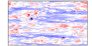
Figure 12 shows the instantaneous  $u^\prime$, i.e. streak structures, at
 $y^+ \approx 1$,
 $6$ and
 $15$ in the uncontrolled and controlled cases. Note that the black line represents the threshold of
 $u^\prime$ to identify the cluster, i.e.
 $u^\prime = - \alpha u^\prime _{rms,NC}$ (see Appendix A for details). As shown in figure 12(
 $a$,
 $b$), in the quite-near-wall region (
 $\kern0.09em y^+ \approx 1$), small-scale structures are dominant in the controlled case. In the region around the virtual wall, i.e.
 $y^+ \approx 6$ (figure 12
 $c$,
 $d$), although the streak structures are suppressed significantly, the small-scale structures are relatively dominant in the controlled case. These small-scale structures make the flow field in the controlled case more complex than that in the uncontrolled case, leading to the increase in
 $H_{sp}$ in the viscous sublayer (
 $\kern0.09em y^+ < 10$). On the other hand, figure 12(
 $e$,
 $f$) shows that the control slightly suppresses the streak structures and decreases the large-scale structures in the streamwise direction. The suppression of the streak structures leads to the slight decrease in the large-scale structures generated by the coalescence of streaks. Subsequently, the small-scale structures generated by the separation of streaks decrease, leading to the decrease in
 $H_{sp}$ in the buffer layer (
 $\kern0.09em y^+ \gtrsim 10$).
Visualisation of instantaneous streamwise velocity fluctuations  $u^\prime$ (streak structures): (
 $a$,
 $b$)
 $y^+ \approx 1$; (
 $c$,
 $d$)
 $y^+ \approx 6$; (
 $e$,
 $f$)
 $\kern0.09em y^+ \approx 15$; (
 $a$,
 $c$,
 $e$) uncontrolled; (
 $b$,
 $d$,
 $f$) opposition (
 $y_d^+ \approx 10$). Colors represents the values of
 $u^\prime$.

To identify the relationship of the variations in  $\tau ^+_{C_{max}}$ and
 $H_{sp}$ with the streak structures in more detail, we investigate the meandering behaviour of streaks in uncontrolled and controlled cases. Note that the detailed methods for quantifying the meandering magnitude and streamwise length of streaks are described in Appendix A. Figure 13 shows the mean meandering magnitudes
 $\overline {\xi _{rms}^+}$ and streamwise length
 $\overline {l_x^+}$ of individual
 $u^\prime$ structures, together with their standard deviations,
 $\sigma _{\xi _{rms}^+}$ and
 $\sigma _{l_x^+}$, respectively. In the uncontrolled case, all these values are small in the viscous sublayer, whereas they rapidly increase in the buffer layer. That is, the meandering magnitude and streamwise length of streaks are small (large) in the viscous sublayer (buffer layer). In addition, we observe a wide variety of meandering magnitudes and streamwise lengths of streaks with increasing
 $y^+$. The active coalescence and separation of streaks in the buffer layer (Smith & Metzler Reference Smith and Metzler1983) increase the variety of streamwise lengths of streaks, and the meandering magnitude of streaks depends on their streamwise length (Bae & Lee Reference Bae and Lee2021; Hwang & Lee Reference Hwang and Lee2022). They are strongly associated with the formation of a wide variety of meandering magnitudes and streamwise lengths of streaks. In the controlled case, all the values shown in figure 13 decrease in the viscous sublayer and buffer layer (especially, in the region below the detection plane, i.e.
 $y ^+ \leq 10$), indicating that the control decreases the variety of meandering magnitudes and streamwise lengths of streaks. This means that the coalescence and separation of streaks are suppressed. The results shown in figures 12 and 13 strongly support the physical mechanism identified by the multiscale CECP and SPE (figure 11).
( $a$) Mean meandering magnitude
 $\overline {\xi ^+_{rms}}$; (
 $b$) mean streamwise length
 $\overline {l_x^+}$; (
 $c$) standard deviation of meandering magnitude
 $\sigma _{\xi ^+_{rms}}$; (
 $d$) standard deviation of streamwise length
 $\sigma _{l_x^+}$; black, uncontrolled; blue, opposition (
 $\kern0.09em y_d^+ \approx 10$).

We here investigate the turbulent energy transport to obtain deeper insights into the drag-reduction mechanism. Figure 14 shows the streamwise components of the production  $P_{u^\prime u^\prime }$ and dissipation
 $\epsilon _{u^\prime u^\prime }$ and the three components of the pressure strain term
 $\varPi ^s_i$. In the viscous sublayer, the enhancement of turbulence by the opposition control leads to the increase in
 $P_{u^\prime u^\prime }$. In addition, the control eliminates the contribution from the viscous diffusion, leading to a significant decrease in the absolute value of
 $\epsilon _{u^\prime u^\prime }$. In the buffer layer, compared with the uncontrolled case,
 $P_{u^\prime u^\prime }$ decreases significantly, whereas the absolute value of
 $\epsilon _{u^\prime u^\prime }$ hardly decreases. This means that the dissipation rate for the generated turbulent energy increases compared with the uncontrolled case. As can be observed in figure 14(
 $b$), the absolute values of the pressure strain in the wall-normal and spanwise directions (
 $\varPi _2^s$ and
 $\varPi _3^s$, respectively) decrease in the viscous sublayer and buffer layer, whereas that in the streamwise direction (
 $\varPi _1^s$) increases (decreases) in the viscous sublayer (buffer layer). The trend of
 $\varPi _1^s$ is similar to that of
 $P_{u^\prime u^\prime }$. In addition, the decreases in the absolute values of
 $\varPi _2^s$ and
 $\varPi _3^s$ indicate that the pressure redistribution of turbulent energy from
 $u^\prime$ to
 $v^\prime$ and
 $w^\prime$ is suppressed, which is related to the regeneration cycle in turbulent flows (Hamilton, Kim & Waleffe Reference Hamilton, Kim and Waleffe1995). Since the wavy motions of streaks (i.e. the streak meandering) plays an important role in this pressure redistribution of turbulent energy (Kawata & Tsukahara Reference Kawata and Tsukahara2021), this is due to the suppression of streak meandering motions shown in figure 13. That is, the opposition control suppresses the regeneration cycle in the region near the wall. This region corresponds reasonably well to the region with actively coalesced and separated streaks that is identified by the multiscale CECP and SPE.
( $a$) Streamwise components of production and dissipation terms; (
 $b$) pressure strain term; no marker, production;
 $\bigcirc$, dissipation;
 $\square$, pressure strain; solid line, streamwise component; dashed line, wall-normal component; dotted line, spanwise component; black, uncontrolled; blue, opposition (
 $\kern0.09em y_d^+ \approx 10$).

Finally, we investigate the Reynolds number effect on the drag-reduction mechanism proposed in this study. Figure 15 shows the variations in  $\tau ^+_{C_{max}}$ and
 $H_{sp}$ as functions of
 $y^+$ in the uncontrolled and controlled cases at a higher Reynolds number of
 $Re_\tau = 590$. Similarly to figure 11, the detection plane is set to
 $y^+_d \approx 10$. The trends shown in figure 15 are very similar to those observed in figure 11. That is, the Reynolds number dependence of the drag-reduction mechanism is relatively small, suggesting that the drag-reduction mechanism proposed in this study is applicable to a wide range of Reynolds numbers.
Variations in  $\tau ^+_{C_{max}}$ and
 $H_{sp}$ as functions of
 $y^+$ at a high Reynolds number of
 $Re_\tau = 590$: (
 $a$)
 $\tau ^+_{C_\textrm {max}}$; (
 $b$)
 $H_{sp}$; black, uncontrolled; blue, opposition (
 $\kern0.09em y_d^+ \approx 10$).

In this study, we have focused mainly on the applicability of the ordinal pattern-based analysis to revealing the drag-reduction mechanism of an opposition-controlled turbulent channel flow. The detection plane has been determined by a phenomenalistic approach based on visualised flow structures (Hammond et al. Reference Hammond, Bewley and Moin1998; Chung & Talha Reference Chung and Talha2011). Other recent studies on opposition control (Stroh et al. Reference Stroh, Frohnapfel, Schlatter and Hasegawa2015; Wang et al. Reference Wang, Choi, Gaster, Atkin, Borodulin and Kachanov2022; Dacome et al. Reference Dacome, Mörsch, Kotsonis and Baars2024) have not provided a methodology to optimise the detection plane. The local link strength in the multivariate OPTN we adopted in this study is an applicable network metric for determining the detection location for opposition control. The drag-reduction effect is significantly associated with the reduction of the region where streaks actively coalesce and separate and the suppression of the regeneration cycle in the region near the wall. To the best of the authors’ knowledge, this is the first study to provide (i) an indicator for appropriately determining the location of the detection plane and (ii) a new interpretation of the drag-reduction mechanism derived from the ordinal pattern-based analysis. In our future work, we will apply the ordinal pattern-based analysis to other control methods and attempt to propose new control strategies.
5. Summary
We have conducted a numerical study on the drag-reduction mechanism of an opposition-controlled turbulent channel flow under a low-Reynolds-number condition from the viewpoint of the symbolic dynamics approach. In this study, we have applied the ordinal pattern-based analysis considering the multivariate OPTN, multiscale CECP and SPE to the flow field with and without the opposition control. The local link strength of the self-loop of nodes representing the negative correlation pattern between  $u^\prime$ and
 $v^\prime$ is predominant in the multivariate OPTN in both the uncontrolled and controlled cases. The effect of the virtual wall generated by the opposition control is maximum at
 $y_d^+ \approx 10$. This location of the detection plane corresponds to the wall-normal location where the local link strength is maximised in the uncontrolled case. These results suggest that the local link strength in the multivariate OPTN has potential use in appropriately determining the location of the detection plane to control a turbulent channel flow. The drag reduction by the opposition control is mainly attributed to the reduction of the region where streaks actively coalesce and separate and the suppression of the regeneration cycle in the region near the wall. This is reasonably identified by the multiscale CECP and SPE.
Acknowledgement
Y.N. is grateful to Dr. H. Mamori (The University of Electro-Communications) for fruitful discussions.
Funding
This study was partially supported by the Ebara Hatakeyama memorial foundation.
Declaration of interests
The authors report no conflict of interest.
Data availability
The data that support the findings of this study are available from the corresponding author upon reasonable request.
Appendix A. Methods for quantifying meandering magnitude and streamwise length of streaks
We apply the cluster detection and conditional sampling techniques to the instantaneous  $u^\prime$ to quantify the meandering magnitude and streamwise length of streaks. Similarly to Hwang & Sung (Reference Hwang and Sung2018) and Hwang & Lee (Reference Hwang and Lee2022), we define the clusters of negative
 $u^\prime$ as the group of connected points satisfying
 \begin{equation} u^\prime <-\alpha u^\prime_{rms,NC}, \end{equation}
where  $u^\prime _{rms,NC}$ is the root mean square (RMS) of
 $u^\prime$ in the uncontrolled case and
 $\alpha$ is the threshold. The threshold
 $\alpha$ can be determined by the percolation analysis (Moisy & Jiménez Reference Moisy and Jiménez2004; del Álamo et al. Reference del Álamo, Jiménez, Zandonade and Moser2006; Lozano-Durán, Flores & Jiménez Reference Lozano-Durán, Flores and Jiménez2012) of the uncontrolled flow field. Figure 16 shows the ratio of the total number of clusters at each
 $\alpha$ to the maximum
 $N$ (
 $N/N_{max}$) identified by percolation analysis, where
 $N$ and
 $N_{max}$ represent the total number of clusters at each
 $\alpha$ and the maximum
 $N$ over
 $\alpha$, respectively. The number of clusters is maximised at
 $\alpha = 1.5$. Thus, we set
 $\alpha = 1.5$.
Ratio of the total number of clusters at each  $\alpha$ to the maximum
 $N$ (
 $N/N_{max}$) identified by percolation analysis (Moisy & Jiménez Reference Moisy and Jiménez2004; del Álamo et al. Reference del Álamo, Jiménez, Zandonade and Moser2006; Lozano-Durán et al. Reference Lozano-Durán, Flores and Jiménez2012).

Subsequently, from the cluster shape identified by (A1), we quantify the meandering magnitude and streamwise length of streaks in each  $x$–
 $z$ plane. Figure 17(
 $a$,
 $b$) shows a three-dimensional view of a cluster extracted from an instantaneous
 $u^\prime$ and a two-dimensional view at
 $y^+ \approx 20$ in (
 $a$), respectively. The light blue region in figure 17(
 $b$) represents the region identified as the cluster at the corresponding
 $y^+$. The spine location
 $z^+_{spine}$ (red solid line) is defined as the mean spanwise location of the light blue region at each streamwise location, i.e.
 \begin{equation} z^+_{spine} = \tfrac{1}{2} (z^+_{max} + z^+_{min}), \end{equation}
where  $z^+_{max}$ and
 $z^+_{min}$ represent the maximum and minimum spanwise locations of the light blue region at each streamwise location, respectively. Then, we obtain the linear fit
 $z^+_{fit}$ (black dash-dotted line) from
 $z^+_{spine}$. The meandering of
 $z^+_{spine}$ (
 $\xi ^+$) is defined as the difference in spanwise location between
 $z^+_{spine}$ and
 $z^+_{fit}$, i.e.
 \begin{equation} \xi^+= z^+_{spine} - z^+_{fit}. \end{equation}
On the basis of the variation in  $\xi ^+$ as a function of
 $x^+$ (figure 17
 $c$), we can quantify the meandering magnitude by measuring the RMS of
 $\xi ^+$ (i.e.
 $\xi ^+_{rms}$). In addition, the difference between the maximum and minimum streamwise locations in the light blue region,
 $x^+_{max}$ and
 $x^+_{min}$, respectively, is defined as the streamwise length
 $l_x^+$ of streaks, i.e.
 \begin{equation} l^+_x=x^+_{max} - x^+_{min}. \end{equation}
Visualisation of a cluster extracted from an instantaneous flow field: ( $a$) three-dimensional view; (
 $b$) two-dimensional view at
 $y^+\approx 20$; (
 $c$) variation in the spine of the streak (
 $\xi ^+=z^+_{spine}-z^+_{fit}$) at
 $y^+\approx 20$. In (
 $b$) and (
 $c$), the red solid line represents the spine of the light blue region (
 $z^+_{spine}$) and the black dash-dotted line represents the linear fit of the spine (
 $z^+_{fit}$).



