1. Introduction
Microstructured optical fibres (MOFs) are a new design of optical fibre which promise the realisation of fibres with effectively any desired optical properties. This flexibility is due to a unique design which employs a series of air channels aligned along the fibre axis to form a waveguide around the core, rather than enclosing the central core with a cladding layer of different material, as is used in regular optical fibres (Knight Reference Knight2003; Monro & Ebendorff-Heidepriem Reference Monro and Ebendorff-Heidepriem2006). Microstructured optical fibres are typically fabricated in two stages. The first stage consists of the construction of a preform between one and three centimetres in diameter, which is a macroscopic version of the final fibre, having the same internal structure. In the second stage, referred to as fibre drawing, the preform is heated and pulled from one end to reduce the outer diameter to between 100 and 200 micrometres and the internal air channels to only a few micrometres to nanometres across. In order to attain the required final geometry it is important to be able to construct a precise preform.
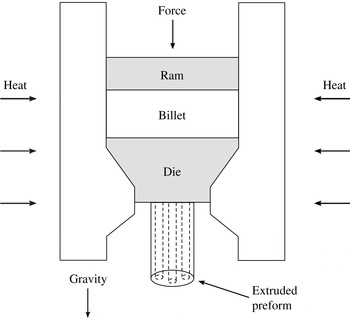
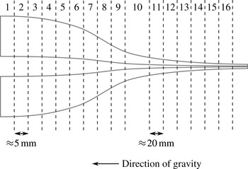
There are several methods available for constructing the preform, including drilling a solid rod or stacking an assembly of capillary tubes. Of particular interest is preform extrusion, which has been shown to be a flexible method of fabrication (Ebendorff-Heidepriem & Monro Reference Ebendorff-Heidepriem and Monro2012). In this method, depicted in figure 1, a piece of material, referred to as a billet and typically a glass, is placed in an extrusion tower and heated. A ram forces the material through a die that contains a number of blocking elements, which form the negative of the desired pattern of air channels. After the molten material passes through the die it leaves the heated region and solidifies. While the desired geometry is specified by the die design, the flow of the molten material in the time between exiting the die and solidification can greatly deform the resulting air channels (Ebendorff-Heidepriem & Monro Reference Ebendorff-Heidepriem and Monro2007). These deformations include changes in the shape and location of the air channels, both of which can render the preform useless. In addition, gravity acts to stretch the extruded preform, which results in a taper. At present, such distortions are accounted for by using repeated trials until the desired geometry is attained.
Schematic of the extrusion process. The billet is heated and forced through the die by the ram. The blocking elements within the die give rise to the pattern of air channels in the preform.

There exists a significant body of work focusing on the second stage of fibre fabrication, the drawing of fluid fibres. Much of this theory stems from the work of Trouton (Reference Trouton1906), who developed a model for the steady stretching of a viscous fibre under gravity. Matovich & Pearson (Reference Matovich and Pearson1969) later extended this model to include surface-tension effects, while Schultz & Davis (Reference Schultz and Davis1982) provided a systematic derivation of this model, making use of a small aspect ratio, and computed higher-order corrections that justified the use of a one-dimensional model. Yarin, Gospodinov & Roussinov (Reference Yarin, Gospodinov and Roussinov1994) found numerical solutions for the drawing of thin-walled cylinders with surface tension and gravity, while Fitt et al. (Reference Fitt, Furusawa, Monro, Please and Richardson2002) investigated the steady-state drawing of capillary tubes through several limiting cases. A review of comparisons between experimental data and slenderness models for fibre drawing has been given by Denn (Reference Denn1980), which showed that one-dimensional models provide a good approximation. Xue et al. (Reference Xue, Tanner, Barton, Lwin, Large and Poladian2005a ,Reference Xue, Tanner, Barton, Lwin, Large and Poladian b , Reference Xue, Large, Barton, Tanner, Poladian and Lwin2006) have used finite element simulations to study several fibre-drawing problems, both steady state and time-dependent. Yarin (Reference Yarin1995) has studied the formation of preforms using layers of materials driven by surface tension without gravity, making use of Fourier expansions to solve the resulting equations. This work assumed that the boundaries of each layer can be represented by small perturbations to circles and made use of a transformed time to link the transverse flow to a uniform axial stretching. It is noted that the equations may also be applied to single-layer preforms. A similar approach to those described above has been used to construct an area-averaged extrusion model (Lin & Jou Reference Lin and Jou1995).
Each of the studies discussed above employed an Eulerian coordinate system; however, many studies of extensional flow, including the present work, make use of a Lagrangian coordinate system (Wilson Reference Wilson1988; Kaye Reference Kaye1991). Lagrangian descriptions have been used to study the gravitational stretching of axisymmetric slender drops neglecting surface tension and inertia (Wilson Reference Wilson1988; Stokes Reference Stokes2000), with inertia (Stokes & Tuck Reference Stokes and Tuck2004) and with surface tension (Wilson Reference Wilson1988; Stokes, Bradshaw-Hajek & Tuck Reference Stokes, Bradshaw-Hajek and Tuck2011). Similar equations also arise in the study of thin sheets of fluid (Wilmott Reference Wilmott1989; Stokes Reference Stokes1999). A slenderness model with a Lagrangian coordinate has been used to study a fibre stretched at both ends (Dewynne, Ockendon & Wilmott Reference Dewynne, Ockendon and Wilmott1989, Reference Dewynne, Ockendon and Wilmott1992); the initial cross-sectional geometry was arbitrary but connected and it was assumed to vary gradually with axial position. A detailed derivation of the leading-order model for drawing, including the effects of both inertia and gravity, has been given by Dewynne, Howell & Willmot (Reference Dewynne, Howell and Willmot1994). Surface tension was neglected in the main text of the paper and it was shown that to leading order the cross-section retains its original shape while its size reduces due to axial stretching. The effect of surface tension is discussed in the appendix but at a magnitude that did not enter the leading-order analysis so that there was no change to the model for the cross-sectional area and axial velocity derived in the paper. It was, however, noted that inclusion of surface tension means that the cross-section no longer retains its initial shape and the shape evolution must be determined by a higher-order transverse-flow model.
Cummings & Howell (Reference Cummings and Howell1999) extended the work of Dewynne et al. (Reference Dewynne, Howell and Willmot1994) to consider surface tension of a magnitude that modifies the leading-order analysis and obtained fully coupled axial- and transverse-flow models in a Lagrangian reference frame, where the transverse-flow model is a two-dimensional Stokes-flow problem with a modified kinematic condition. They made the critical observation that a transformation of the time variable reduces the transverse-flow model to a classical two-dimensional Stokes-flow problem with unit surface tension that is independent of the axial-flow model. This transverse model can be solved once for a given initial cross-sectional shape, and yields the evolution of the geometry (shape) of the cross-section. The area of each cross-section evolves according to the one-dimensional axial-flow model, which has an additional term (not found in the Dewynne et al. (Reference Dewynne, Howell and Willmot1994) model) that depends upon surface tension and the boundary length from the transverse-flow problem. Cummings & Howell (Reference Cummings and Howell1999) do not describe their method of solution of the axial-flow problem using the boundary length from the transverse problem except to indicate that this was done by transformation back to the physical time and Lagrangian space variables. A similar method has been used to model the drawing of a thin-walled tube (a viscida) by Griffiths & Howell (Reference Griffiths and Howell2007, Reference Griffiths and Howell2008, Reference Griffiths and Howell2009). Chakravarthy & Chiu (Reference Chakravarthy and Chiu2009) applied the slenderness model of Cummings & Howell (Reference Cummings and Howell1999) in the Eulerian reference frame to the drawing of fibres with multiply connected cross-sectional geometries, and investigated the relative effects of surface tension, axial inertia and gravity. The transverse and axial problems, which in the Eulerian formulation are fully coupled, were solved simultaneously via a numerical procedure. Stokes et al. (Reference Stokes, Buchak, Crowdy and Ebendorff-Heidepriem2014) investigated the drawing of a preform into a fibre neglecting gravitational effects and showed that the Lagrangian formulation of the problem, together with application to the axial problem of the time transformation introduced by Cummings & Howell (Reference Cummings and Howell1999), enabled an explicit description of the solution to the axial stretching problem in terms of the evolution of the cross-sectional geometry given by the solution of the transverse problem for any initial geometry.
As a first step to understanding MOF preform extrusion we here consider the simpler problem of the stretching under gravity of a cylindrical fluid region with internal structure and surface tension. It will be assumed that the molten material can be modelled as a Newtonian fluid and that, over the time scales of interest, inertia is negligible. We demonstrate that the results of Stokes et al. (Reference Stokes, Buchak, Crowdy and Ebendorff-Heidepriem2014) may be extended to model the stretching under gravity of a slender fluid region of arbitrary cross-section, so that the transverse flow decouples from the axial flow in an identical manner and evolves as a two-dimensional Stokes flow with unit surface tension. The key differences are that the axial flow is no longer steady and the area evolution equation depends upon the initial position of each cross-section.
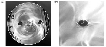
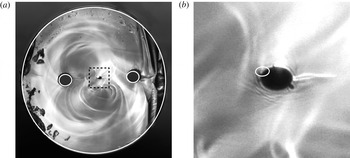
A particular focus of the present work is to analyse the interaction between gravitational and surface-tension forces. Specifically, we wish to determine if and when surface-tension effects are important. It has been shown by Wylie, Huang & Miura (Reference Wylie, Huang and Miura2011) that for the pulling by a fixed force of a solid axisymmetric viscous thread with small inertia the effect of surface tension is negligible. Experiments by the authors reported here show that the inner boundaries of fluid regions with interior structure undergo some deformation that is not explained by axial stretching but is explained by surface tension. As an example of these experiments, figure 2 shows a preform that originally contained three circular inner boundaries that was fixed at one end and heated so that it stretched under gravity. It should be noted that the central hole has become elliptical. This is similar to the deformations observed in MOF preform extrusion (Monro & Ebendorff-Heidepriem Reference Monro and Ebendorff-Heidepriem2006). Shown overlaid on this image is the best match produced by our model, which shows good qualitative agreement. The model and this experiment will be discussed further below.
It will be shown that the importance of surface tension depends upon both the relevant dimensionless parameters and the geometry under consideration. Furthermore, the influence of surface tension on both the axial and transverse flows must be considered, and is investigated through several limiting cases. Particular attention is given to geometries with internal structure.
This paper is structured as follows. Section 2 considers the derivation of a model for a stretching fluid region. General solutions are presented both with and without surface-tension effects. In § 3 we present solutions for several example geometries with no internal boundaries and use these to illustrate the effect of surface tension. Solutions with internal holes are discussed in § 4 and are compared with experimental data. The implications of these results are discussed in § 5, along with future work to be undertaken.
Photograph of a cross-section from a cylinder with three holes that has stretched under gravity. The diameter of the cylinder is approximately
 $677~{\rm\mu}\text{m}$
, while the region inside the square from the photograph in (a) is shown approximately eight times larger in (b). The central hole appears to show deformation consistent with surface-tension effects. This is similar to behaviour observed in MOF preform extrusion. Shown overlaid is the best match from the model, which displays good qualitative agreement.

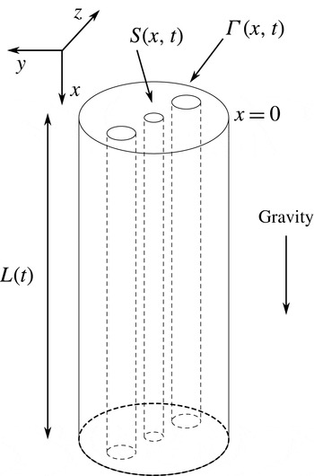
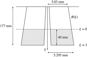
A typical cylinder with internal structure. A Cartesian coordinate system is employed in which the
 $x$
-axis is directed along the axis of the cylinder, while the
 $y$
- and
 $z$
-axes are oriented in the transverse direction. The length and cross-sectional area are denoted
 $L(t)$
and
 $S(x,t)$
respectively. The total boundary length of each cross-section is denoted
 ${\it\Gamma}(x,t)$
. The cylinder is aligned such that gravity acts in the direction of increasing
 $x$
.

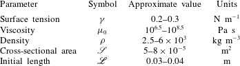
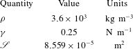
Typical parameter values for gravitational extension of a fluid cylinder.

2. The mathematical model
2.1. Formulation
Consider a tube with some internal structure, as shown in figure 3, which is labelled by a Cartesian coordinate system in which the
 $x$
-axis is directed vertically down along the cylinder axis, while the
 $y$
- and
 $z$
-axes lie in the transverse plane. The corresponding velocity vector is denoted
 $(u,v,w)$
and the pressure
 $p$
. The length is denoted
 $L(t)$
, while the cross-section at position
 $x$
and time
 $t$
has area
 $S(x,t)$
. The total perimeter of each cross-section is denoted
 ${\it\Gamma}(x,t)$
. Since the cylinder is fixed at the top we specify that
 $u(0,t)=0$
, while the initial profile
 $S_{0}(x)=S(x,0)$
and initial length
 $L_{0}=L(0)$
are also known. We point out that both the initial cross-sectional area and the shape may vary with position
 $x$
, i.e. they are not necessarily uniform.
Table 1 shows some typical parameter values for the gravitational extension problem here considered, which are also relevant to MOF preform extrusion. The area
 $\mathscr{S}$
represents a typical cross-sectional area; often
 $S_{0}$
is constant and
 $\mathscr{S}=S_{0}$
. The length scale
 $\mathscr{L}$
is usually the initial length of the cylinder, i.e.
 $\mathscr{L}=L_{0}$
. From these values we observe that the slenderness parameter
 ${\it\epsilon}=\sqrt{\mathscr{S}}/\mathscr{L}$
is no larger than
 $0.3$
and we shall assume that
 ${\it\epsilon}$
is
 $O(10^{-1})$
. We thus introduce the scaled quantities denoted by carets:
 $$\begin{eqnarray}\displaystyle \left.\begin{array}{@{}c@{}}\displaystyle (x,y,z)=\mathscr{L}(\hat{x},{\it\epsilon}{\hat{y}},{\it\epsilon}\hat{z}),\quad t=\frac{\mathscr{L}}{U}\hat{t},\quad (u,v,w)=U(\hat{u} ,{\it\epsilon}\hat{v},{\it\epsilon}{\hat{w}}),\\ \displaystyle S=\mathscr{S}{\hat{S}},\quad {\it\Gamma}={\it\epsilon}\mathscr{L}\hat{{\it\Gamma}},\quad p=\frac{{\it\mu}_{0}U}{\mathscr{L}}\hat{p}.\end{array}\right\} & & \displaystyle\end{eqnarray}$$
Here,
 $U={\it\rho}g\mathscr{L}^{2}/{\it\mu}_{0}$
is a velocity scale chosen to balance viscous stresses and gravity, where
 ${\it\rho}$
is the fluid density,
 ${\it\mu}_{0}$
is a typical viscosity and
 $g$
is gravity. At leading order in
 ${\it\epsilon}$
the temperature is constant within any cross-section (Huang et al.
Reference Huang, Wylie, Miura and Howell2007), so that the temperature of the cylinder is assumed to vary with axial position and time. Since the viscosity depends only upon temperature we assume that the viscosity is also constant within any cross-section and write
 ${\it\mu}(x,t)={\it\mu}_{0}{\it\mu}^{\ast }(\hat{x},\hat{t})$
, where
 ${\it\mu}^{\ast }$
is the scaled quantity. The surface tension
 ${\it\gamma}$
and density
 ${\it\rho}$
are both assumed to be independent of temperature and are taken to be constant along the length of the tube. In order for surface-tension effects to appear in the leading-order problem we introduce the scaled surface tension
 ${\it\gamma}^{\ast }={\it\gamma}/{\it\mu}_{0}U{\it\epsilon}$
, which is assumed to be
 $O(1)$
.
Since the viscosity depends upon the temperature we must solve for the latter in order to determine the former. This necessitates the inclusion of an energy conservation equation coupled to the fluid flow equations, such as the one-dimensional models employed by Yarin et al. (Reference Yarin, Rusinov, Gospodinov and Radev1989), Huang et al. (Reference Huang, Wylie, Miura and Howell2007), Griffiths & Howell (Reference Griffiths and Howell2008) and Taroni et al. (Reference Taroni, Breward, Cummings and Griffiths2013), and the deformation and stretching of the cylinder will depend on the temperature, which will depend on the cylinder geometry. This is a non-trivial matter, and the addition of a coupled energy equation to the model is left to future work. For this study we focus on the solution of the momentum equations, giving these and, as much as possible, expressing solutions in terms of a general viscosity function
 ${\it\mu}^{\ast }(x,t)$
. Ultimately, for generating results we will assume that the viscosity is constant so that
 ${\it\mu}^{\ast }\equiv 1$
. Moreover, we will show that we are able to use experimental data to validate our flow-modelling approach and investigate the importance of surface tension in a way that accounts for the temperature varying viscosity independently of the model, albeit, as will be seen, the
 $x$
dependence of the cylinder geometry as given by model and experiment cannot be compared, which, in any case, was not possible due to a lack of the experimental measurements needed for this.
Returning to the flow model, each of the unknown variables is expanded as a power series in
 ${\it\epsilon}^{2}$
. As per Cummings & Howell (Reference Cummings and Howell1999), this expansion results in coupled systems for the axial and transverse flows, which are discussed in the following subsections.
2.2. Axial problem
The axial flow is described by equations governing conservation of both mass and momentum expressed in terms of the area
 ${\hat{S}}$
and boundary length
 $\hat{{\it\Gamma}}$
. These equations have been previously derived by Cummings & Howell (Reference Cummings and Howell1999). Dropping carets from scaled variables but retaining asterisks on scaled parameters for later convenience, the mass and momentum equations are respectively
 $$\begin{eqnarray}\displaystyle & \displaystyle S_{t}+(uS)_{x}=0, & \displaystyle\end{eqnarray}$$
 $$\begin{eqnarray}\displaystyle & \displaystyle ReS(u_{t}+uu_{x})-(3{\it\mu}^{\ast }Su_{x})_{x}=Sg^{\ast }+\frac{{\it\gamma}^{\ast }}{2}{\it\Gamma}_{x}. & \displaystyle\end{eqnarray}$$
Here, we have introduced the Reynolds number
 $Re={\it\rho}U\mathscr{L}/{\it\mu}_{0}$
and scaled gravity
 $$\begin{eqnarray}\displaystyle g^{\ast }=\frac{{\it\rho}g\mathscr{L}^{2}}{{\it\mu}_{0}U}=\frac{Re}{Fr^{2}}, & & \displaystyle\end{eqnarray}$$
where
 $Fr=U/\sqrt{g\mathscr{L}}$
is the Froude number. Setting
 $U={\it\rho}g\mathscr{L}^{2}/{\it\mu}_{0}$
(as given earlier) yields
 $g^{\ast }=1$
. This choice also yields the dimensionless parameters
 $$\begin{eqnarray}\displaystyle Re=\frac{{\it\rho}^{2}g\mathscr{L}^{3}}{{\it\mu}_{0}^{2}},\quad {\it\gamma}^{\ast }=\frac{{\it\gamma}}{{\it\rho}g\mathscr{L}\sqrt{\mathscr{S}}}. & & \displaystyle\end{eqnarray}$$
The dimensionless surface tension
 ${\it\gamma}^{\ast }$
is an inverse Bond number. Using the typical parameter values from table 1,
 $Re$
is at most
 $O(10^{-9})$
, justifying neglect of the inertial terms on the left-hand side of (2.3) until a sufficiently long time has elapsed that accelerations throughout the fluid cylinder approach gravitational acceleration, when this approximation is no longer valid (Stokes & Tuck Reference Stokes and Tuck2004; Wylie et al.
Reference Wylie, Huang and Miura2011). However, as this is not a feature of the problems and time scales of interest here we consider only the case of negligible inertia. The dimensionless surface tension is
 $O(10^{-1})$
, and, while this appears small, we do not drop this term in the governing equations in order to investigate the effect of surface tension. It will later be shown that surface tension must be included in order to capture the behaviour observed in experiments.
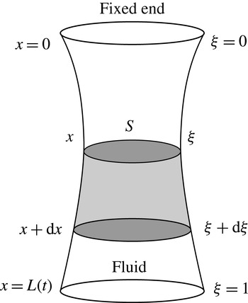
The axial coordinate
 $x$
, shown on the left-hand side of the diagram, is converted to the Lagrangian coordinate
 ${\it\xi}$
, shown on the right, defined by the initial position of each cross-section so that
 ${\it\xi}=x({\it\xi},0)$
. By requiring conservation of mass within the shaded region and taking the limit as its length is reduced to zero we obtain the relationship between the two coordinates.

Introducing the material derivative
 $\text{D}S/\text{D}t=\partial S/\partial t+uS_{x}$
, we write (2.2) in the form
 $$\begin{eqnarray}\displaystyle \frac{\text{D}S}{\text{D}t}=-Su_{x}, & & \displaystyle\end{eqnarray}$$
which is substituted into (2.3) to eliminate the axial velocity
 $u$
. It is useful to introduce the axial Lagrangian coordinate
 ${\it\xi}=x({\it\xi},0)$
, where
 $x({\it\xi},t)$
is the position of cross-section
 ${\it\xi}$
at time
 $t$
and
 ${\it\xi}$
is the initial position of each cross-section; the relation between
 $x$
and
 ${\it\xi}$
is illustrated in figure 4. As per Stokes & Tuck (Reference Stokes and Tuck2004), conservation of mass requires that the Eulerian and Lagrangian coordinates are related by
 $$\begin{eqnarray}\displaystyle S({\it\xi},t)\frac{\partial x}{\partial {\it\xi}}=S({\it\xi},0), & & \displaystyle\end{eqnarray}$$
or, equivalently,
 $$\begin{eqnarray}\displaystyle x({\it\xi},t)=\int _{0}^{{\it\xi}}\frac{S_{0}({\it\xi}^{\prime })}{S({\it\xi}^{\prime },t)}\,\text{d}{\it\xi}^{\prime }. & & \displaystyle\end{eqnarray}$$
Writing (2.3) in terms of the Lagrangian variable and integrating with respect to
 ${\it\xi}$
yields
 $$\begin{eqnarray}\displaystyle 3{\it\mu}^{\ast }\frac{\text{D}S}{\text{D}t}=-V({\it\xi})+\frac{{\it\gamma}^{\ast }}{2}{\it\Gamma}-c(t), & & \displaystyle\end{eqnarray}$$
where
 $$\begin{eqnarray}\displaystyle V({\it\xi})=\int _{{\it\xi}}^{1}S_{0}({\it\xi}^{\prime })\,\text{d}{\it\xi}^{\prime } & & \displaystyle\end{eqnarray}$$
is the dimensionless weight of fluid between cross-section
 ${\it\xi}$
and the lower end of the cylinder. The function
 $c(t)$
is a possibly time-dependent axial tension within the fluid that is determined by the boundary condition at the bottom of the cylinder. For a uniform initial geometry
 $S({\it\xi},0)\equiv 1$
, so that
 $V({\it\xi})=1-{\it\xi}$
. In the case of a solid axisymmetric cylinder (2.9) is identical to that found by Stokes et al. (Reference Stokes, Bradshaw-Hajek and Tuck2011, equation (8), p. 324). In the absence of any external pulling of the cylinder, we assume that
 $c(t)=0$
(corresponding to zero stress) and that any change in cross-sectional area at the very bottom of the cylinder where
 $V({\it\xi})=0$
is due to surface tension. As will be seen in § 4, experiments show that the cross-sectional area at the very bottom of the cylinder changes very little with time. In some practical applications the cylinder is pulled with a constant force and
 $c(t)$
will be a positive constant, although a time-dependent force is also possible for preform extrusion which motivates this work, as well as for fibre drawing.
We also note that under the slenderness assumption the sides of the fluid region are taken to have small slope so that there is no axial contribution to the curvature. At the free end of the cylinder
 ${\it\xi}=1$
; however, surface tension will work to round the sharp corners and this free end will no longer be flat. In this study we ignore this effect, which occurs over a long time relative to the stretching time, noting that it will have a negligible impact on the rest of the fluid away from
 ${\it\xi}=1$
.
At present, (2.9) involves two dependent unknown variables
 $S$
and
 ${\it\Gamma}$
. For a general geometry there is no simple relationship between the area of each cross-section and the total boundary length, so that at present the problem is not closed. In order to relate these two quantities we must make use of the transverse problem, discussed in the following subsection.
2.3. Transverse problem
Again following Cummings & Howell (Reference Cummings and Howell1999), the transverse-flow problem is readily solved by considering the flow at each Lagrangian coordinate
 ${\it\xi}$
and scaling the cross-plane coordinates by
 $\sqrt{S({\it\xi},t)}$
, so that
 $(y,z)=\sqrt{S}({\tilde{y}},\tilde{z})$
and
 ${\it\Gamma}=\sqrt{S}\tilde{{\it\Gamma}}({\it\xi},t)$
. We also rescale the pressure and velocity, defining
 $$\begin{eqnarray}\displaystyle p=\bar{p}+\frac{{\it\gamma}^{\ast }}{\sqrt{S}}\tilde{p},\quad (v,w)=(\bar{v},\bar{w})+\frac{{\it\gamma}^{\ast }}{{\it\mu}^{\ast }}(\tilde{v},\tilde{w}), & & \displaystyle\end{eqnarray}$$
where
 $\bar{p}$
and
 $(\bar{v},\bar{w})$
comprise the zero-surface-tension eigensolution given by Dewynne et al. (Reference Dewynne, Howell and Willmot1994), who showed that with no surface tension each cross-section changes in scale but not shape. Then, only the components of the pressure and velocity due to surface tension (
 $\tilde{p},\tilde{v}$
and
 $\tilde{w}$
) will feature in the transverse problem. We emphasise that, because the initial cross-sectional shape may vary with axial position, there is, potentially, a different transverse problem for every cross-section
 ${\it\xi}$
, because the initial condition is different. This means that every dependent variable in the transverse problem must be labelled by
 ${\it\xi}$
, a feature of the transverse-flow model developed here that is not seen in the model of Stokes et al. (Reference Stokes, Buchak, Crowdy and Ebendorff-Heidepriem2014) for fibre drawing, nor even in that of Cummings & Howell (Reference Cummings and Howell1999) which includes gravity. For a uniform cross-sectional geometry the transverse-flow problem is the same for every cross-section.
Following each cross-section, the transverse flow due to surface tension is governed by the equations
 $$\begin{eqnarray}\displaystyle \tilde{v}_{{\tilde{y}}}+\tilde{w}_{\tilde{z}} & \hspace{-2.0pt}=\hspace{-2.0pt} & \displaystyle 0,\end{eqnarray}$$
 $$\begin{eqnarray}\displaystyle \tilde{v}_{{\tilde{y}}{\tilde{y}}}+\tilde{v}_{\tilde{z}\tilde{z}} & \hspace{-2.0pt}=\hspace{-2.0pt} & \displaystyle \tilde{p}_{{\tilde{y}}},\end{eqnarray}$$
 $$\begin{eqnarray}\displaystyle \tilde{w}_{{\tilde{y}}{\tilde{y}}}+\tilde{w}_{\tilde{z}\tilde{z}} & \hspace{-2.0pt}=\hspace{-2.0pt} & \displaystyle \tilde{p}_{\tilde{z}},\end{eqnarray}$$
 $$\begin{eqnarray}\displaystyle ({\it\mu}^{\ast }\sqrt{S}/{\it\gamma}^{\ast })G_{t}+\tilde{v}G_{{\tilde{y}}}+\tilde{w}G_{\tilde{z}} & \hspace{-2.0pt}=\hspace{-2.0pt} & \displaystyle 0\quad \text{on }G=0,\end{eqnarray}$$
 $$\begin{eqnarray}\displaystyle G_{{\tilde{y}}}(-\tilde{p}+2\tilde{v}_{{\tilde{y}}})+G_{\tilde{z}}(\tilde{v}_{\tilde{z}}+\tilde{w}_{{\tilde{y}}}) & \hspace{-2.0pt}=\hspace{-2.0pt} & \displaystyle -\tilde{{\it\kappa}}G_{{\tilde{y}}}\quad \text{on }G=0,\end{eqnarray}$$
 $$\begin{eqnarray}\displaystyle G_{{\tilde{y}}}(\tilde{v}_{\tilde{z}}+\tilde{w}_{{\tilde{y}}})+G_{\tilde{z}}(-\tilde{p}+2\tilde{w}_{\tilde{z}}) & \hspace{-2.0pt}=\hspace{-2.0pt} & \displaystyle -\tilde{{\it\kappa}}G_{\tilde{z}}\quad \text{on }G=0,\end{eqnarray}$$
 $G=0$
is the boundary of each cross-section, which may consist of multiple pieces that are not connected. Equations (2.12a
–
c
) are simply the two-dimensional Stokes equations, while (2.12e
,
f
) are the dynamic boundary conditions for unit surface tension. The remaining kinematic condition (2.12d
) is transformed into a standard kinematic boundary condition by introducing the reduced time (Griffiths & Howell Reference Griffiths and Howell2008; Stokes et al.
Reference Stokes, Buchak, Crowdy and Ebendorff-Heidepriem2014)
 $$\begin{eqnarray}\displaystyle {\it\tau}({\it\xi},t)={\it\gamma}^{\ast }\int _{0}^{t}\frac{1}{{\it\mu}^{\ast }\sqrt{S}}\,\text{d}t^{\prime }, & & \displaystyle\end{eqnarray}$$
which is here labelled with cross-sectional position
 ${\it\xi}$
, yielding
 $$\begin{eqnarray}\displaystyle G_{{\it\tau}}+\tilde{v}G_{{\tilde{y}}}+\tilde{w}G_{\tilde{z}}=0\quad \text{on }G=0. & & \displaystyle\end{eqnarray}$$
Thus, with this transformation, the cross-flow becomes a classical unit-surface-tension-driven free-boundary Stokes-flow problem with unit area. There are a variety of methods available for solving such a problem. For example, Hopper (Reference Hopper1990) presented exact solutions for a selection of connected domains, while problems featuring domains of higher connectivity may be solved using numerical methods (Buchak et al. Reference Buchak, Crowdy, Stokes and Ebendorff-Heidepriem2015).
The key observation to be made is that the transverse problem for cross-section
 ${\it\xi}$
is independent of the axial flow. The consequence of this is that, for any given geometry, we can solve the transverse-flow problem for each
 ${\it\xi}$
without any knowledge of the axial flow, and this solution alone governs the shape of the cross-section. Any change over time in the viscosity of the cross-section
 ${\it\mu}^{\ast }({\it\xi},t)$
is accounted for by the new time variable
 ${\it\tau}$
. This decoupling of the transverse flow from the axial flow also occurs in fibre drawing (Stokes et al.
Reference Stokes, Buchak, Crowdy and Ebendorff-Heidepriem2014), but is in contrast to the work of Chakravarthy & Chiu (Reference Chakravarthy and Chiu2009), who did not transform to reduced time and instead used an unmodified kinematic condition, equivalent to (2.12d
), which does depend on the axial problem. Once each transverse problem is solved we can readily calculate the scaled boundary length
 $\tilde{{\it\Gamma}}({\it\xi},{\it\tau})$
. The process of coupling the two problems and using viscosity information to determine the physical geometry is discussed below.
2.4. Coupling
To make use of the transverse solution for cross-section
 ${\it\xi}$
, we first transform (2.9) to reduced time
 ${\it\tau}$
. Making this transformation, the time-dependent tension
 $c(t)$
becomes a function
 $B$
of both
 ${\it\xi}$
and
 ${\it\tau}$
; at a given
 $t$
, the reduced time
 ${\it\tau}$
varies with
 ${\it\xi}$
so that
 $c(t)=B({\it\xi},{\it\tau})$
. With the scaled boundary length
 $\tilde{{\it\Gamma}}({\it\xi},{\it\tau})$
known from the transverse problem, the unscaled boundary length is given by
 ${\it\Gamma}({\it\xi},{\it\tau})=\sqrt{S({\it\xi},{\it\tau})}\,\tilde{{\it\Gamma}}({\it\xi},{\it\tau})$
. Making these substitutions yields
 $$\begin{eqnarray}\displaystyle \frac{3{\it\gamma}^{\ast }}{\sqrt{S}}\frac{\text{D}S}{\text{D}{\it\tau}}=-V+\frac{{\it\gamma}^{\ast }}{2}\sqrt{S}\tilde{{\it\Gamma}}-B. & & \displaystyle\end{eqnarray}$$
We define
 $$\begin{eqnarray}\displaystyle 6{\it\sigma}^{\ast }({\it\xi},{\it\tau})=V({\it\xi})+B({\it\xi},{\it\tau}), & & \displaystyle\end{eqnarray}$$
which represents the total dimensionless tension, due to gravity and any additional pulling, acting on cross-section
 ${\it\xi}$
at reduced time
 ${\it\tau}$
. Finally, introducing
 ${\it\chi}=\sqrt{S}$
and rearranging yields
 $$\begin{eqnarray}\displaystyle \frac{\text{D}{\it\chi}}{\text{D}{\it\tau}}-\frac{1}{12}{\it\chi}\tilde{{\it\Gamma}}=-\frac{{\it\sigma}^{\ast }}{{\it\gamma}^{\ast }}. & & \displaystyle\end{eqnarray}$$
This is a linear ordinary differential equation in
 ${\it\chi}$
, which corresponds to that seen in fibre drawing, except that
 ${\it\sigma}^{\ast }$
is not constant but dependent on
 ${\it\xi}$
and
 ${\it\tau}$
. As in Stokes et al. (Reference Stokes, Buchak, Crowdy and Ebendorff-Heidepriem2014), it may be solved by introducing the integrating factor
 $$\begin{eqnarray}\displaystyle H({\it\xi},{\it\tau})=\exp \left(-\frac{1}{12}\int _{0}^{{\it\tau}}\tilde{{\it\Gamma}}({\it\xi},{\it\tau}^{\prime })\,\text{d}{\it\tau}^{\prime }\right), & & \displaystyle\end{eqnarray}$$
which yields the solution
 $$\begin{eqnarray}\displaystyle {\it\chi}({\it\xi},{\it\tau})=\frac{1}{H}\left({\it\chi}_{0}({\it\xi})-\frac{1}{{\it\gamma}^{\ast }}\int _{0}^{{\it\tau}}{\it\sigma}^{\ast }H\,\text{d}{\it\tau}^{\prime }\right). & & \displaystyle\end{eqnarray}$$
Here, we have introduced
 ${\it\chi}_{0}({\it\xi})={\it\chi}({\it\xi},0)$
, which is the initial value of
 ${\it\chi}$
. For a cylinder with initially uniform cross-section,
 ${\it\chi}_{0}({\it\xi})=\sqrt{S_{0}({\it\xi})}\equiv 1$
. While (2.19) is similar in form to that previously obtained for the drawing of fibres (Stokes et al.
Reference Stokes, Buchak, Crowdy and Ebendorff-Heidepriem2014, equation (2.19), p. 183), it differs significantly in that
 ${\it\sigma}^{\ast }$
is not a constant but, in general, a function of both
 ${\it\xi}$
and
 ${\it\tau}$
because of the inclusion of gravity and the time-dependent tension
 $B({\it\xi},{\it\tau})$
. Ultimately, we will assume that
 $B({\it\xi},{\it\tau})$
is constant, in which case (2.19) differs from the solution for fibre drawing only because
 ${\it\sigma}^{\ast }$
and, possibly,
 ${\it\chi}_{0}$
depend on
 ${\it\xi}$
, so that a different solution
 ${\it\chi}$
is obtained for each
 ${\it\xi}$
. In general, (2.19) has no exact solution and we must compute the integrals in (2.18) and (2.19) numerically.
Given some cross-section
 ${\it\xi}$
and reduced time
 ${\it\tau}$
, we use (2.19) to compute the area of the cross-section, while the solution to the transverse problem determines the shape of the cross-section. Thus, these two solutions together completely describe how cross-section
 ${\it\xi}$
evolves in
 ${\it\tau}$
. To determine the physical cylinder geometry at physical time
 $t$
we require a relationship between
 $t$
and
 ${\it\tau}$
for each
 ${\it\xi}$
. This is obtained by rearranging (2.13) to give
 $$\begin{eqnarray}\displaystyle \int _{0}^{{\it\tau}}{\it\chi}\,\text{d}{\it\tau}^{\prime }=\int _{0}^{t}\frac{{\it\gamma}^{\ast }}{{\it\mu}^{\ast }}\,\text{d}t^{\prime }=\frac{{\it\gamma}^{\ast }t}{m({\it\xi},t)}, & & \displaystyle\end{eqnarray}$$
where
 $m({\it\xi},t)$
is the harmonic mean of
 ${\it\mu}^{\ast }({\it\xi},t)$
at position
 ${\it\xi}$
over time
 $t$
. It is left to future work to couple solution of (2.20) with a temperature model to properly determine the physical geometry, so, at present, we will simply assume a viscosity profile
 ${\it\mu}^{\ast }$
and, hence,
 $m$
. We note that when
 ${\it\mu}^{\ast }={\it\mu}^{\ast }({\it\xi})$
we have
 $m=m({\it\xi})={\it\mu}^{\ast }({\it\xi})$
. Substituting (2.19) into (2.20) gives the relationship between
 $t$
and
 ${\it\tau}$
at each cross-section
 ${\it\xi}$
. At a given
 $t>0$
the dependence of (2.20) on
 ${\it\xi}$
means that
 ${\it\tau}$
will differ from cross-section to cross-section so that each will have a different shape, even in the case that
 ${\it\chi}_{0}$
is independent of
 ${\it\xi}$
. This is in contrast to previous models of fibre drawing (Stokes et al.
Reference Stokes, Buchak, Crowdy and Ebendorff-Heidepriem2014), in which every cross-section has the same initial geometry and evolves over the same reduced time
 ${\it\tau}$
as it is drawn, and so has the same shape. If required, the Eulerian position
 $x$
at any time
 $t$
may be determined by substituting
 $S={\it\chi}^{2}$
into (2.8), which will typically need to be evaluated numerically.
Summarising, the general solution procedure is as follows.
-
(i) Solve the transverse-flow problem for each
 ${\it\xi}$
.
-
(ii) Calculate
$\tilde{{\it\Gamma}}({\it\xi},{\it\tau})$
from the cross-flow solution and, hence,
$H({\it\xi},{\it\tau})$
from (2.18). -
(iii) Calculate
${\it\chi}({\it\xi},{\it\tau})$
from (2.19). -
(iv) For each time
$t$
of interest:-
(1) find
${\it\tau}$
for each cross-section
${\it\xi}$
using (2.20); -
(2) evaluate
$S({\it\xi},{\it\tau})$
and
$x({\it\xi},{\it\tau})$
.
-


The time dependence of
 $c(t)$
greatly increases the difficulty of this problem. In typical MOF preform extrusion there is a constant pulling force and very often
 $c(t)\equiv 0$
. From this point onwards we will assume that
 $c(t)=B({\it\xi},{\it\tau})=c$
is constant.
2.5. Solution for weak surface tension
Previously it was assumed that
 ${\it\gamma}^{\ast }$
was
 $O(1)$
and a solution was derived that included the surface-tension terms, which we will refer to as the full solution. It was observed, however, that
 ${\it\gamma}^{\ast }$
is
 $O(10^{-2})$
or smaller, which suggests that surface tension has only a small effect on the solution. To investigate the importance of surface tension we here consider two approximations to the full problem. If
 ${\it\gamma}^{\ast }\ll 1$
, the surface-tension terms from the axial equation (2.9) may be dropped, so that this equation no longer depends upon the transverse problem. In addition, if
 ${\it\gamma}^{\ast }=0$
then (2.13) implies that
 ${\it\tau}=0$
and the transverse problem may be neglected. This agrees with results observed by Dewynne et al. (Reference Dewynne, Howell and Willmot1994) for fibre drawing, namely that without surface tension the cross-sections would change scale due to stretching but remain the same shape. We will refer to this as the zero-surface-tension (ZST) case. If
 ${\it\gamma}^{\ast }\ll 1$
but the area
 $S$
is small, so that the term
 ${\it\gamma}^{\ast }/\sqrt{S}$
from the integrand in (2.13) is
 $O(1)$
, then
 ${\it\tau}$
will not necessarily be small and each cross-section may still undergo a significant shape change. Furthermore, if the cross-sectional geometry has large curvatures then even small values of
 ${\it\tau}$
may mean a significant change to the cross-sectional shape. To investigate these possibilities we also consider the solution when surface-tension terms are neglected in the axial problem but the transverse problem is retained, which is denoted the weak-surface-tension (WST) case. The importance of the size of
 ${\it\gamma}^{\ast }$
relative to
 $S$
and the curvature is investigated in detail in the following sections by comparing solutions with the full, ZST and WST models.
Both the ZST and WST cases share the same axial equation (2.9) with the surface-tension term removed. Integrating yields
 $$\begin{eqnarray}\displaystyle S({\it\xi},t)=S_{0}({\it\xi})-\frac{2t{\it\sigma}^{\ast }({\it\xi})}{m({\it\xi},t)}. & & \displaystyle\end{eqnarray}$$
We note that the ZST–WST solution for
 $S$
does not depend on the cross-sectional shape, i.e.
 ${\it\Gamma}({\it\xi},{\it\tau})$
, which is in contrast to the solution of the full problem. For the WST case we can also obtain an expression for
 $S$
at each
 ${\it\xi}$
in terms of
 ${\it\tau}$
. From (2.17), and neglecting the term involving
 $\tilde{{\it\Gamma}}$
, we find
 $$\begin{eqnarray}\displaystyle {\it\chi}({\it\xi},{\it\tau})={\it\chi}_{0}({\it\xi})-\frac{{\it\sigma}^{\ast }({\it\xi}){\it\tau}}{{\it\gamma}^{\ast }}. & & \displaystyle\end{eqnarray}$$
Equating with (2.21) gives the relationship between
 $t$
and
 ${\it\tau}$
,
 $$\begin{eqnarray}\displaystyle \frac{t{\it\gamma}^{\ast }}{m({\it\xi},t)}={\it\tau}\left({\it\chi}_{0}-\frac{{\it\sigma}^{\ast }{\it\tau}}{2{\it\gamma}^{\ast }}\right). & & \displaystyle\end{eqnarray}$$
Writing (2.23) as a quadratic polynomial in
 ${\it\tau}$
and solving for
 ${\it\tau}$
gives
 $$\begin{eqnarray}\displaystyle {\it\tau}=\frac{{\it\gamma}^{\ast }}{{\it\sigma}^{\ast }}\left[{\it\chi}_{0}-\left({\it\chi}_{0}^{2}-\frac{2{\it\sigma}^{\ast }t}{m}\right)^{1/2}\right], & & \displaystyle\end{eqnarray}$$
where we must use the negative square root so that
 $\partial {\it\tau}/\partial t>0$
and
 ${\it\tau}({\it\xi},0)=0$
. Thus, the WST solution, if appropriate, provides a straightforward relation between
 ${\it\tau}$
and
 $t$
.
For the special case in which the viscosity
 ${\it\mu}^{\ast }$
and initial area
 $S_{0}$
are independent of
 ${\it\xi}$
further progress can be made. For
 $t>0$
, substituting for
 $S({\it\xi},t)$
in (2.8) and integrating yields
 $$\begin{eqnarray}\displaystyle x({\it\xi},t)=\frac{3m}{t}\log \left(1+\frac{t{\it\xi}}{3m-t(1+c)}\right), & & \displaystyle\end{eqnarray}$$
where
 $m=m(t)$
. Setting
 ${\it\xi}=1$
we find that the length of the fluid region is given by
 $$\begin{eqnarray}\displaystyle x(1,t)=L(t)=\frac{3m}{t}\log \left(1+\frac{t}{3m-t(1+c)}\right). & & \displaystyle\end{eqnarray}$$
Rearranging (2.25), it may be shown that
 $$\begin{eqnarray}\displaystyle \left[1-\frac{t(1+c)}{3m}\right]\exp \left(\frac{tx}{3m}\right)=1-\frac{t(1-{\it\xi}+c)}{3m}. & & \displaystyle\end{eqnarray}$$
Observing that the right-hand side of this expression matches the right-hand side of (2.21) we may eliminate
 ${\it\xi}$
to obtain
 $$\begin{eqnarray}\displaystyle S(x,t)=\left[1-\frac{t(1+c)}{3m}\right]\exp \left(\frac{tx}{3m}\right),\quad 0\leqslant x\leqslant L(t). & & \displaystyle\end{eqnarray}$$
This provides a full solution to the ZST case. For the WST case we must, in addition, solve the transverse problem and relate
 $t$
to
 ${\it\tau}$
. From (2.24) we have
 $$\begin{eqnarray}\displaystyle {\it\tau}=\frac{{\it\gamma}^{\ast }}{{\it\sigma}^{\ast }({\it\xi})}\left[1-\left(1-2\frac{{\it\sigma}^{\ast }({\it\xi})\,t}{m}\right)^{1/2}\right]. & & \displaystyle\end{eqnarray}$$
3. Cylinders with no internal structure
In this section we consider some illustrative solutions for the stretching under gravity of cylinders with no internal structure. The effect of surface tension, in terms of both the cross-sectional geometry and the magnitude of the surface-tension parameter, is investigated by comparing solutions of the full problem with those obtained assuming zero and weak surface tension for two different geometries, namely a solid axisymmetric rod and a cylinder with a non-circular epicycloid cross-section. We will examine how well the ZST and WST solutions represent the full problem solution relative to the magnitude of the surface-tension parameter for
 ${\it\gamma}^{\ast }=10^{-3},10^{-2}$
and
 $10^{-1}$
. For generality, solutions are derived as far as possible for a viscosity that varies with both Lagrangian coordinate
 ${\it\xi}$
and time
 $t$
, but all results presented are for a constant viscosity.
The circular rod does not evolve in the transverse-flow problem and has axial solution
 $$\begin{eqnarray}\displaystyle {\it\chi}=\left({\it\chi}_{0}-\frac{{\it\sigma}^{\ast }}{{\it\delta}}\right)\text{e}^{{\it\tau}\sqrt{{\rm\pi}}/6}+\frac{{\it\sigma}^{\ast }}{{\it\delta}}, & & \displaystyle\end{eqnarray}$$
where
 ${\it\delta}={\it\gamma}^{\ast }\sqrt{{\rm\pi}}/6$
. To relate
 $t$
and
 ${\it\tau}$
we substitute
 ${\it\chi}$
from (3.1) into (2.20), which yields the algebraic relationship
 $$\begin{eqnarray}\displaystyle \frac{6}{\sqrt{{\rm\pi}}}\left({\it\chi}_{0}-\frac{{\it\sigma}^{\ast }}{{\it\delta}}\right)(\text{e}^{{\it\tau}\sqrt{{\rm\pi}}/6}-1)+\frac{{\it\sigma}^{\ast }}{{\it\delta}}{\it\tau}=\frac{{\it\gamma}^{\ast }}{m({\it\xi},t)}t. & & \displaystyle\end{eqnarray}$$
An exact solution to the transverse problem for the evolution of an epicycloid was given by Hopper (Reference Hopper1990), and substitution of this into (2.20) gives the relation between
 $t$
and
 ${\it\tau}$
via numerical integration. We here set
 $c=0$
.
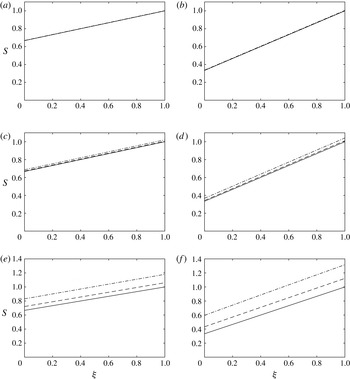
Figure 5 shows the area
 $S$
plotted against
 ${\it\xi}$
at times
 $t=1$
and
 $2$
for each of the selected values of
 ${\it\gamma}^{\ast }$
for the ZST–WST problem (in which
 $S$
is independent of the cross-sectional geometry) and for the full problem, where the cross-section is a circle and an epicycloid. From these curves it can be seen that when
 ${\it\gamma}^{\ast }=10^{-3}$
all three solutions are identical to graphical accuracy at both times. This suggests that for this value of
 ${\it\gamma}^{\ast }$
surface tension does not have a significant effect, regardless of the geometry under consideration. For
 ${\it\gamma}^{\ast }=10^{-2}$
the three solutions show qualitative but not quantitative agreement. At
 $t=1$
the ZST–WST solution and solid-rod solution are similar, while the epicycloid solution has a larger area at all values of
 ${\it\xi}$
. By time
 $t=2$
, the rod has deviated from the ZST–WST solution by more, while the epicycloid solution is further away again. Finally, with
 ${\it\gamma}^{\ast }=10^{-1}$
, the differences are even more pronounced and are clearly visible at both times. Once again, the epicycloid solution is larger than that for the rod, which is in turn larger than the ZST–WST solution. The differences between the rod and epicycloid may be explained by the difference in the boundary lengths. The initial boundary length of the epicycloid is greater than that of the circle and remains larger over the course of this simulation. On inspecting (2.9), it is clear that the larger
 $\tilde{{\it\Gamma}}$
is, the greater the influence of surface tension is on the axial problem. The ZST–WST solution is smallest as it has no boundary length term. As these differences accumulate with time the deviation is greater at
 $t=2$
than at
 $t=1$
.
Within the transverse problem surface tension works to reduce the total boundary length, so that as
 ${\it\tau}$
increases
 $\tilde{{\it\Gamma}}$
decreases towards
 $2\sqrt{{\rm\pi}}$
, which is the total boundary length for a disk of unit area. In addition, as a given cross-section
 ${\it\xi}$
becomes smaller due to axial stretching the unscaled boundary length
 ${\it\Gamma}$
must also decrease, so that the influence of surface tension on
 $S$
decreases with time. In regions near the end of the cylinder
 ${\it\xi}=1$
, where there is little stretching,
 $S$
increases with time, which is most noticeable for larger
 ${\it\gamma}^{\ast }$
. The scaled boundary length
 $\tilde{{\it\Gamma}}$
still decreases with
 ${\it\tau}$
but
 ${\it\Gamma}=\sqrt{S}\tilde{{\it\Gamma}}$
may increase due to the increase in
 $S$
. On differentiating (2.13) with respect to
 $t$
we observe that as
 $S$
increases the rate of increase in
 ${\it\tau}$
reduces. Thus, surface tension works to slow the rate of change of
 ${\it\tau}$
.
The solutions
 $S({\it\xi},t)$
corresponding to the ZST–WST solution (solid curve), and the full problem for both the rod (dashed curve) and the epicycloid (dash–dot curve). The solutions have been computed with dimensionless surface tensions
 ${\it\gamma}^{\ast }=10^{-3}$
,
 $10^{-2}$
and
 $10^{-1}$
, and are shown at times
 $t=1$
and
 $2$
: (a)
 ${\it\gamma}^{\ast }=10^{-3},t=1$
; (b)
 ${\it\gamma}^{\ast }=10^{-3},t=2$
; (c)
 ${\it\gamma}^{\ast }=10^{-2},t=1$
; (d)
 ${\it\gamma}^{\ast }=10^{-2},t=2$
; (e)
 ${\it\gamma}^{\ast }=10^{-1},t=1$
; (f)
 ${\it\gamma}^{\ast }=10^{-1},t=2$
. For
 ${\it\gamma}^{\ast }=10^{-3}$
the three solutions are indistinguishable to graphical accuracy at both times shown. For
 ${\it\gamma}^{\ast }=10^{-2}$
the epicycloid solution is slightly larger for all
 ${\it\xi}$
, while the rod and ZST–WST solutions remain similar to each other. For
 ${\it\gamma}^{\ast }=10^{-1}$
the three solutions differ noticeably. The difference between the epicycloid and rod solutions is due to the longer boundary of the epicycloid. The magnitude of the difference between solutions increases with time.

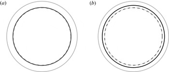
The influence of surface tension may also be observed in the cross-section profiles. In the case of the rod the shape of each cross-section remains the same in the transverse problem and can only change in scale due to axial stretching. Figure 6 shows cross sections through the rod at
 ${\it\xi}=0.5$
at
 $t=2$
for
 ${\it\gamma}^{\ast }=10^{-2}$
and
 $10^{-1}$
. For the smaller value of
 ${\it\gamma}^{\ast }$
the ZST, WST and full solutions have all changed in scale due to axial stretching but are otherwise indistinguishable. For
 ${\it\gamma}^{\ast }=10^{-1}$
the ZST and WST solutions still appear identical, while the full solution is noticeably larger. These results all agree with the corresponding plots of
 $S$
shown in figures 5(d) and 5(f) respectively. Thus, without any transverse evolution the cross-section is completely described by the axial solution. For
 ${\it\gamma}^{\ast }\leqslant 10^{-2}$
there is no noticeable difference between the solutions, while by
 ${\it\gamma}^{\ast }=10^{-1}$
the full solution differs due to reduced axial stretching on account of the surface-tension term in the axial equation.
The cross-section at
 ${\it\xi}=0.5$
for the stretching circular cylinder. The initial condition is shown in solid grey. At
 $t=2$
we have the full solution (solid black), the WST solution (black dashed) and the ZST solution (grey dotted). The solutions are indistinguishable at
 ${\it\gamma}^{\ast }=10^{-2}$
(a), while for
 ${\it\gamma}^{\ast }=10^{-1}$
(b) the full solution is significantly different from the ZST and WST solutions, which are identical.

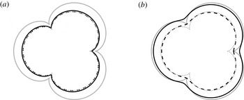
In the case of the epicycloid there are some notable differences in behaviour due to surface-tension-driven flow in the cross-section. Again, we consider cross-sections at
 ${\it\xi}=0.5$
and
 $t=2$
, which are plotted in figure 7. At
 ${\it\gamma}^{\ast }=10^{-2}$
the ZST and WST solutions are practically identical, while the full solution shows some smoothing at the cusps and is larger in the regions between. For
 ${\it\gamma}^{\ast }=10^{-1}$
the three solutions are all distinct. The full solution shows further smoothing and has not reduced much in area. The WST solution shows similar smoothing but, without the resistance to gravity provided by surface tension in the axial problem, has reduced in scale. While the ZST solution has the same area as the WST solution, it has a noticeably different shape as there is no surface-tension-driven flow in the transverse direction to smooth the cusps.
The cross-section at
 ${\it\xi}=0.5$
for the stretching epicycloid cylinder. The initial condition is shown in solid grey. At
 $t=2$
we have the full solution (solid black), the WST solution (black dashed) and the ZST solution (grey dotted). The solutions are similar for
 ${\it\gamma}^{\ast }=10^{-2}$
(a) but are all distinct for
 ${\it\gamma}^{\ast }=10^{-1}$
(b).

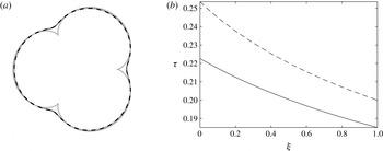
The effect of surface tension can be further highlighted by comparing the domains from the transverse problem so that they each have unit area, which allows a comparison between the solutions without the effect of axial stretching. Figure 8(a) shows such a comparison for the epicycloid at
 $t=2$
and
 ${\it\gamma}^{\ast }=10^{-1}$
, from which it is evident that the full and WST solutions show almost identical behaviour, while the ZST and initial condition are necessarily identical. To see why the full and WST solutions agree, the values of
 ${\it\tau}$
from these two solutions are plotted against
 ${\it\xi}$
in figure 8(b). While the two curves clearly differ at the plotted scale, this difference is never more than
 $3.09\times 10^{-2}$
, which occurs at
 ${\it\xi}=0$
. The shapes for the full and WST problems are thus effectively the same. Hence, even though
 ${\it\tau}$
depends upon
 $S$
, as can be seen from (2.13), the different axial solutions from the full and WST problems make little difference to the value of
 ${\it\tau}$
and hence the shape observed; rather, the shape differs depending on the magnitude of surface tension in the transverse problem.
Comparison between the solutions to the transverse (scaled) problem with
 ${\it\gamma}^{\ast }=10^{-1}$
. (a) Cross-sections at
 ${\it\xi}=0.5$
and
 $t=2$
for the initial condition (grey solid), which is also the ZST solution, the full solution (solid black) and the WST solution (grey dashed); the full and WST solutions appear almost identical. (b) The values of
 ${\it\tau}$
for the full (solid black) and WST (black dashed) problems, which differ by at most
 $3.09\times 10^{-2}$
.

For the two cylinders considered in this subsection we have seen that for
 ${\it\gamma}^{\ast }$
 $O(10^{-3})$
surface tension does not have a significant impact on either the axial or transverse systems and the ZST model provides a good approximation to the full problem. If
 ${\it\gamma}^{\ast }$
is
 $O(10^{-2})$
the ZST–WST axial model shows small differences from the full model but still provides a useful approximation. At this value of
 ${\it\gamma}^{\ast }$
all three transverse models show close agreement; the ZST model differs in regions of large curvature. For
 ${\it\gamma}^{\ast }$
of
 $O(10^{-1})$
the WST transverse model still provides a good approximation to the full problem; however, the ZST–WST axial model and ZST transverse model show significant differences and are no longer appropriate.
4. Cylinders with internal structure: model and experiment
4.1. Overview and experimental set-up
In this section we solve for the gravitational stretching, with no additional forcing (i.e.
 $c=0$
), of fluid cylinders with internal structure; that is, having interior boundaries. Two cases are considered: (1) a cylinder with an annular cross-section, for which an exact solution exists, and (2) a circular cylinder with three circular holes having collinear centres on a diameter of the cross-section, for which a numerical solution is obtained.
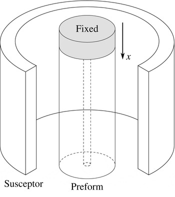
An experiment was also conducted for each of these cases. The experimental procedure is described in detail in appendix A, but a brief summary is given here. The cylinders were made from glass and each was placed into an optical fibre-drawing tower with the top end fixed and the bottom end free, as shown for an annular tube in figure 9. The cylinder was heated by a surrounding susceptor and the softened cylinder was stretched under gravity so that it extended below the susceptor, where it cooled. After some minutes the bottom metre or so was broken off, which consisted of a drop connected to a tapered filament, which we call ‘the drop’. Experimental data were obtained from this piece, consisting of the initial and final geometries of, and the weight below, a number of cross-sections.
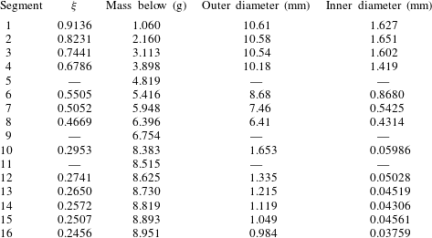
From the weight below a cross-section the corresponding Lagrangian coordinate
 ${\it\xi}$
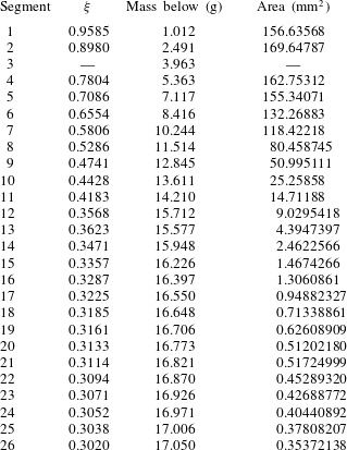
was calculated, as described in appendix A, where the experimental measurements are also given. The known weights
 ${\it\sigma}({\it\xi})$
and surface tension
 ${\it\gamma}$
allow the computation of the ratio
 ${\it\sigma}^{\ast }/{\it\gamma}^{\ast }={\it\sigma}/(6{\it\gamma}\sqrt{\mathscr{S}})$
, which is needed in the model. For each
 ${\it\xi}$
the model gives both the area and the shape of the cross-section as a function of the reduced-time variable
 ${\it\tau}$
, while the experiment gives both the area and the shape of the cross-section at the end of the experiment. To compare the model and the experimental data at Lagrangian position
 ${\it\xi}$
, we use the experimentally measured cross-sectional area
 $S$
to determine the reduced time
 ${\it\tau}$
corresponding to the end of the experiment and then compare the cross-sectional geometry at that
 ${\it\tau}$
as given by the model with that seen experimentally. That is, we are able to calculate the predicted shape of each cross-section given the observed area. In effect, this removes the axial stretching from both the model and the data, allowing a comparison of the transverse surface-tension-driven flow. As we will see, the shape of the interior boundaries can be explained only with the inclusion of the surface-tension-driven transverse problem. Comparisons are made with the full and WST models.
Schematic showing the experimental set-up for the annular tube. The upper end of a glass tube was held fixed while the lower end was free. The glass was heated by the surrounding electromagnetically heated susceptor and allowed to stretch under gravity. In the diagram a section of the susceptor has been removed for clarity. The lower portion of the cylinder that deforms has a length somewhat less than the length of the susceptor.

As already noted previously, a more complete comparison of the cylinder geometry as given by the model with that obtained experimentally requires knowledge of the viscosity (or temperature) of the glass. In addition to the coupling of a thermal model with the flow model, experimental information is needed to establish the exact initial length
 $\mathscr{L}$
of the cylinder and the physical time from the commencement of deformation to the end of the experiment. This is left to future work.
4.2. Stretching annular tube
As a first example of a geometry with internal structure we consider a cylinder in which each cross-section is an annulus. Both the size and the aspect ratio of the annulus are allowed to vary with
 ${\it\xi}$
. The transverse problem admits an exact solution and, following Stokes et al. (Reference Stokes, Buchak, Crowdy and Ebendorff-Heidepriem2014), yields the axial solution
 $$\begin{eqnarray}\displaystyle {\it\chi}=\left(\frac{{\it\tau}}{2{\it\alpha}_{0}}+1\right)^{1/3}\left\{{\it\chi}_{0}({\it\xi})-\frac{3{\it\alpha}_{0}{\it\sigma}^{\ast }}{{\it\gamma}^{\ast }}\left[\left(\frac{{\it\tau}}{2{\it\alpha}_{0}}+1\right)^{2/3}-1\right]\right\}, & & \displaystyle\end{eqnarray}$$
where
 ${\it\alpha}_{0}({\it\xi})$
is the difference between the scaled outer and inner radii at position
 ${\it\xi}$
and reduced time
 ${\it\tau}=0$
. Although the axial solution (4.1) is expressed most simply in terms of the parameter
 ${\it\alpha}_{0}$
, extruded annular preforms are more commonly described by the aspect ratio
 ${\it\phi}$
of the inner to outer radii. The quantities
 ${\it\alpha}_{0}$
and
 ${\it\phi}_{0}={\it\phi}({\it\xi},0)=\text{constant}$
are related by
 $$\begin{eqnarray}\displaystyle {\it\alpha}_{0}^{2}=\frac{1-{\it\phi}_{0}}{{\rm\pi}(1+{\it\phi}_{0})}. & & \displaystyle\end{eqnarray}$$
Using (2.20) it may be shown that
 $t$
and
 ${\it\tau}$
at cross-section
 ${\it\xi}$
are related by the algebraic equation
 $$\begin{eqnarray}\displaystyle \frac{2{\it\gamma}^{\ast }}{3{\it\alpha}_{0}m({\it\xi},t)}t=\left({\it\chi}_{0}({\it\xi})+\frac{3{\it\alpha}_{0}{\it\sigma}^{\ast }}{{\it\gamma}^{\ast }}\right)\left[\left(\frac{{\it\tau}}{2{\it\alpha}_{0}}+1\right)^{4/3}-1\right]-\frac{{\it\sigma}^{\ast }{\it\tau}}{{\it\gamma}^{\ast }}\left(\frac{{\it\tau}}{2{\it\alpha}_{0}}+2\right). & & \displaystyle\end{eqnarray}$$
With this solution we are now in a position to investigate the influence of surface tension on a stretching tube. For this we again assume a constant viscosity, so that
 ${\it\mu}\equiv m\equiv 1$
, and consider a cylinder with
 ${\it\chi}_{0}({\it\xi})=1$
and constant
 ${\it\alpha}_{0}({\it\xi})$
. We consider annuli with initial aspect ratios
 ${\it\phi}_{0}$
between
 $0.2$
and
 $0.9$
in steps of
 $0.1$
. For each
 ${\it\phi}_{0}$
we compute the geometry at
 $t=1$
for
 ${\it\gamma}^{\ast }=10^{-2}$
and
 $10^{-1}$
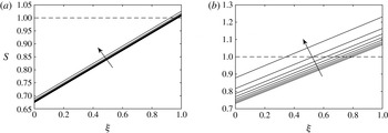
. The computed areas
 $S$
are plotted in figure 10. Although the aspect ratio varies with
 ${\it\xi}$
and
 $t$
, the mass below each cross-section
 ${\it\xi}$
remains unchanged over time, allowing a comparison of surface-tension effects alone. For both values of
 ${\it\gamma}^{\ast }$
the area at
 $t=1$
increases with the initial aspect ratio. This is because the surface-tension component (
 ${\it\gamma}^{\ast }{\it\Gamma}/2$
) in (2.9) that opposes gravitational stretching increases with
 ${\it\phi}$
, since
 ${\it\Gamma}$
increases with
 ${\it\phi}$
. Clearly a larger surface tension
 ${\it\gamma}^{\ast }$
also increases
 $S({\it\xi},t)$
.
The area
 $S({\it\xi},t)$
plotted against
 ${\it\xi}$
for an annulus with
 $S_{0}({\it\xi})=1$
. Solutions are shown at time
 $t=1$
for initial aspect ratios
 ${\it\phi}_{0}=0.2,0.3,\ldots ,0.9,$
and
 ${\it\gamma}^{\ast }=10^{-2}$
(a) and
 $10^{-1}$
(b). The initial condition is shown as a dashed line while the arrows indicate the direction of increasing
 ${\it\phi}_{0}$
. For both values of
 ${\it\gamma}^{\ast }$
the area increases at every value of
 ${\it\xi}$
as
 ${\it\phi}_{0}$
increases. The increase is greater for larger
 ${\it\gamma}^{\ast }$
.

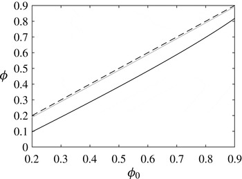
The function
 ${\it\phi}({\it\xi},1)$
describes the shape, i.e. aspect ratio, at
 $t=1$
of each cross-section, independent of any change of scale due to stretching. For any initial value
 ${\it\phi}_{0}$
, the aspect ratio by time
 $t=1$
changes little with
 ${\it\xi}$
. The solid curves in figure 11 show
 ${\it\phi}(0.5,1)$
plotted against
 ${\it\phi}_{0}$
for
 ${\it\gamma}^{\ast }=10^{-2}$
and
 $10^{-1}$
; the line shown dashed is that applicable to the case of zero surface tension and, hence, no change over time from
 ${\it\phi}_{0}$
. As can be seen across all values of
 ${\it\phi}_{0}$
, for
 ${\it\gamma}^{\ast }=10^{-2}$
the aspect ratio does not change significantly from the initial value and hence surface tension has little influence on the transverse flow. In contrast, for
 ${\it\gamma}^{\ast }=10^{-1}$
the ratio decreases for all initial conditions
 ${\it\phi}_{0}$
by approximately
 $0.1$
due to surface tension; there is a slightly smaller decrease for
 ${\it\phi}_{0}>0.8$
. Thus, even though the value of
 ${\it\tau}$
depends upon
 $S$
via (2.13), which from figure 10 changes significantly with
 ${\it\xi}$
, the shape of each cross-section shows little dependence upon
 ${\it\xi}$
and is influenced largely by the value of
 ${\it\gamma}^{\ast }$
alone.
The aspect ratios
 ${\it\phi}$
of the annuli from the transverse problem at
 ${\it\xi}=0.5$
and
 $t=1$
plotted against the initial value
 ${\it\phi}_{0}$
for
 ${\it\gamma}^{\ast }=10^{-2}$
(solid grey) and
 ${\it\gamma}^{\ast }=10^{-1}$
(solid black). For comparison, the line
 ${\it\phi}={\it\phi}_{0}$
is also plotted (dashed). For
 ${\it\gamma}^{\ast }=10^{-2}$
the ratio does not change significantly from the initial value, while for
 ${\it\gamma}^{\ast }=10^{-1}$
it has decreased by approximately
 $0.1$
across all values of
 ${\it\phi}_{0}$
.

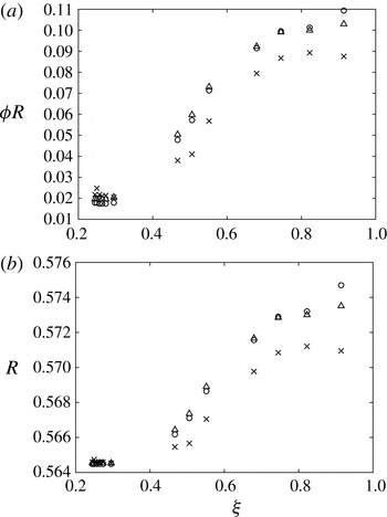
To conclude our examination of the stretching annular tube we compare our model with experimental data. A complete description of the experiment, including the procedure, measurements taken and sources of error, is lengthy and is found in appendix A. Briefly, an annular tube with aspect ratio
 ${\it\phi}_{0}=0.168$
and a nominal initial external radius of 5 mm was fixed in a fibre-drawing tower, heated, and allowed to stretch under gravity; see figure 9. By matching experimentally measured cross-sectional areas to the model we find the value
 ${\it\tau}$
corresponding to each cross-section, and this is used in the transverse model to predict the cross-section geometry. That is, we are able to calculate the shape of each cross-section given the predicted area and compare the shape with that seen experimentally. The experimental external and internal radii scaled with
 $\sqrt{\mathscr{S}S({\it\xi},t)}$
, denoted
 $R$
and
 ${\it\phi}R$
, are plotted for some different values of
 ${\it\xi}$
in figure 12 along with the theoretical radii from the transverse problem for both the full and WST solutions. Since the scaled radii from the experimental data differ from their initial value, while in the absence of surface tension these should remain unchanged, we conclude that surface tension is having a significant effect. This deformation is larger as
 ${\it\xi}$
decreases, which is due to two effects: (1) the cross-sections with smaller label
 ${\it\xi}$
spent longer in the heated susceptor region and hence had more chance to deform, and (2) due to stretching under a larger gravitational force they became smaller, giving rise to higher curvatures and hence a stronger surface-tension effect. For both the inner and outer radii the qualitative match between the models and experiment is very good. In the region
 ${\it\xi}<0.4$
each segment adds only a very small weight so that there is little change in the total axial force (weight) below each cross-section (see table 3, segments 10–16) and the radii change very little with
 ${\it\xi}$
.
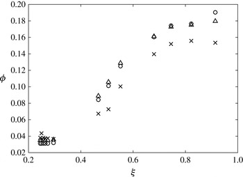
Figure 13 shows the aspect ratio
 ${\it\phi}$
from the data and as predicted by the full and WST models. There is a strong dependence of
 ${\it\phi}$
on
 ${\it\xi}$
. As commented earlier, this dependence is not seen in model results obtained assuming a constant viscosity. It is due rather to the changes in viscosity that occur as the glass cools.
There are several potential sources of error in the experimental data. Both boundaries are not perfectly circular so that the diameters measured vary depending on the orientation of the cross-section. It is also difficult to identify the precise location of the boundary, particularly when measuring the internal hole. Values measured using photographs can be incorrect if the camera is not correctly aligned, resulting in a skewed image. This is of particular importance for
 ${\it\xi}<0.4$
, for which both diameters were measured using photographs. Taking into account these possible errors, the theoretical and observed values show good qualitative agreement. From this we conclude that the model is capturing the important physics in the problem. Importantly, the reduction in radius observed in figure 12, when axial stretching has been removed, can only be explained by surface tension. We must include surface tension in order to capture the correct shape in each cross-section.
The dimensionless (a) inner radius
 ${\it\phi}R$
and (b) outer radius
 $R$
for the stretching annular tube. Shown are the experimental data (crosses), and the predictions by the full (circles) and WST (triangles) models. Both models produce similar results and provide a very good qualitative match to the data. In the absence of surface tension the cross-section in the transverse-flow model will not change over time, so that the reduction in radius can only be explained by surface tension.

The aspect ratio
 ${\it\phi}$
for the stretching annular tube. Shown are the experimental data (crosses), and the predictions by the full (circles) and WST (triangles) models. The value of
 ${\it\phi}$
shows a strong dependence upon
 ${\it\xi}$
, which is due to a varying viscosity.

4.3. Three-hole experiment
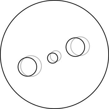
We now consider a similar experiment to that in the previous section but with the multiply connected cross-section geometry shown in figure 14. This has a circular outer boundary with three circular inner holes and is of interest as it is similar to the shape of MOF preforms used for electro-optic fibre designs (Manning Reference Manning2011). The cylinder was produced by drilling the three internal channels into a solid rod. The top and bottom of the drilled cylinder are shown overlaid in figure 14. Unfortunately, the axes of the channels were not exactly parallel to the axis of the cylinder, while in neither the top nor the bottom cross-section was the centre of the middle hole at the centre of the outer boundary. As the experimental data recorded corresponded to a portion of the cylinder at the bottom, the lower geometry was used as the initial condition for the model. Relative to this, the central hole in the upper cross-section is translated by 8 % of the cylinder radius while the outer holes are translated by approximately 14 % of the cylinder radius. We estimate that all experimental data correspond to cross sections with an initial geometry that differs from the initial condition used (i.e. the lower cross-section) by less than 2 %. Evaluation of (2.19), as well as determination of the cross-sectional shape, required the solution of the transverse-flow problem, and with no exact solution available, this was done numerically using a complex-variable-based spectral method similar to that of Buchak et al. (Reference Buchak, Crowdy, Stokes and Ebendorff-Heidepriem2015), which has been described by Tronnolone (Reference Tronnolone2016).
Initial configuration for the three-channel cylinder. The traces of the bottom (dark) and top (light) cross-sections are shown overlaid. The bottom geometry was used as the initial condition in the transverse problem.

Cross-section
 ${\it\xi}=0.3020$
with the predicted shape from the model, corresponding to
 ${\it\tau}=0.091$
, overlaid in white. The diameter of the cylinder is approximately
 $677~{\rm\mu}\text{m}$
, while the region inside the square from the photograph in (a) is shown approximately eight times larger in (b). The two outer holes show good agreement in both shape and size. While the predicted size of the central hole does not match exactly, the model does capture the correct qualitative behaviour.

To provide a representative example of this process we here consider the predicted cross-section at
 ${\it\xi}=0.3020$
. Using the measured cross-sectional area to determine
 ${\it\tau}$
as described above and in appendix A yields the value
 ${\it\tau}\approx 0.091$
, corresponding to the geometry shown in figure 15, while the WST model predicts the reduced time
 ${\it\tau}=0.089$
, which corresponds to an almost identical geometry (not shown). The two outer holes are almost circular but have decreased in size, while the central hole has both decreased in size and also become elliptical. This shows very good qualitative agreement with the observed geometry, also shown in figure 15; however, the model predicts a smaller central hole than that observed in the experiment.
By comparing the solution to the transverse problem with the experimental result graphically, the best match occurs at the reduced time
 ${\it\tau}=0.08$
, which is shown in figure 2. At this value of
 ${\it\tau}$
the interior holes predicted by the model are of similar size and shape to those observed in the experiment. Allowing for experimental error and the method used for determining
 ${\it\tau}$
, the model captures the correct behaviour very well.
This comparison of model and experiment demonstrates the importance of surface tension. Without surface tension the cross-sections will change in scale only but will undergo no other deformation. Experimentally, however, the central hole is seen to become elliptical in shape, matching the expected shape produced by the model with surface tension driving the transverse flow. Thus, surface tension must be included in order to correctly model the transverse flow. This is particularly important for the smaller central hole, which has the highest curvature of the four boundaries.
5. Conclusions
We have developed a model for the gravitational stretching of fluid cylinders with internal structure. The time scales of interest are such that inertia is negligible. This model can be applied to any cross-sectional geometry provided that it is possible to solve the associated transverse Stokes-flow problem. For some cases, such as those illustrated in § 3 and the annulus from § 4, exact solutions exist, otherwise this problem must be solved using numerical methods.
While the full model includes surface-tension effects in both the axial and the transverse problem, it is possible to derive simplified models with surface tension featuring only in the transverse problem (the WST case) or neglected altogether (the ZST case). For typical values of the surface-tension parameter
 ${\it\gamma}^{\ast }$
of size
 $O(10^{-2})$
it has been shown that surface tension does not have a strong influence on the axial problem; however, for the transverse flow surface tension is important in regions of high curvature. When
 ${\it\gamma}^{\ast }$
is
 $O(10^{-1})$
surface tension is important in the axial problem. This theoretical result is supported by the experimental data. To capture the correct behaviour it was essential to include surface tension in the transverse problem. The reduced-time model provided a convenient mechanism for estimating the transverse flow without knowledge of the viscosity.
The stretching under gravity of a fluid cylinder with internal structure and surface tension was investigated here because it closely resembles the conditions experienced by an MOF preform after the material exits the die. Due to this similarity, it is likely that surface tension is also important to understanding the extrusion of MOFs. To further investigate this hypothesis, future work will extend this model by including the addition of material at the top of the cylinder, with the ultimate aim of developing a model of the MOF extrusion process.
Previous work (Huang et al. Reference Huang, Wylie, Miura and Howell2007) has shown that, under a slenderness approximation, the temperature is a function of axial position and time only. As viscosity depends on temperature we must determine the latter in order to compute the former using a viscosity–temperature relationship appropriate to the material from which the cylinder is made. However, in this work, while we have given the model and experimental solutions in terms of a general viscosity function, all model results have been obtained using a constant viscosity. As a consequence, while we have been able to show excellent agreement between our model and experiments with respect to the cross-sectional shape of a cylinder stretched by gravity, we are not in a position to compare between our model and experiments with respect to the change in geometry with axial position. In theory, the temperature may be found using a one-dimensional heat model coupled to the fluid flow, and this has been left to future work. We note also that more work is needed in the future to obtain experimental information on the temperature profile, which is also needed for a complete comparison of our model with experiments.
As already mentioned, this study has concerned only situations in which inertia is not important, and we emphasise that inertia is not important in the experiments described above. Given sufficient time, however, a cylinder may stretch and thus reduce sufficiently in diameter so that the original length scales are no longer appropriate and accelerations become comparable to gravity. In this case the problem enters a new regime in which the Reynolds number may no longer be assumed small, so that inertial effects become important. Wylie & Huang (Reference Wylie and Huang2007) have studied this phenomenon in some detail, while the inclusion of inertia has also been investigated in the absence of surface tension by Stokes & Tuck (Reference Stokes and Tuck2004). It is possible to extend the methods discussed here by retaining the inertial terms in the axial problem; however, this leads to a more complicated equation that has no known explicit solution and presents significant challenges even for a numerical solution. Under a ZST or WST approximation it is possible to derive a diffusion-like axial equation similar to that of Stokes & Tuck (Reference Stokes and Tuck2004). The investigation of such a modification is left to future work.
Acknowledgements
H.T. was supported by an Australian Postgraduate Award and the A. F. Pillow Applied Mathematics Top-Up Scholarship. The research was also supported by grant DP130101541 from the Australian Research Council. It was in part performed at the Optofab node of the Australian National Fabrication Facility utilising Commonwealth and SA State Government funding. The authors wish to thank D. G. Crowdy for useful discussions.
Appendix A. Experimental set-up and measurements
A.1. General method
A cylinder of F2 lead silicate glass from the Schott Glass Company (2015) with a known geometry was placed into an optical fibre-drawing tower with the top end fixed and the bottom end free, as shown for an annular tube in figure 9. The cylinder was surrounded by an electromagnetically heated susceptor that was initially at room temperature and then heated to 930 °C so that the glass softened and the tube stretched under gravity, with no additional pulling. After some minutes the cylinder had deformed such that a drop was suspended by a thin filament, several metres in length, extending back to the remainder of the cylinder at the top of the drawing tower. The bottom metre or so, which by this time had cooled sufficiently to solidify and handle, was broken off. All data were obtained from this piece, which consisted of a drop connected to a tapered filament and which we hereafter simply call ‘the drop’.
When completely cold, the drop was weighed and then divided into segments, as illustrated in figure 16. The segments closest to the free end of the drop were each approximately 5 mm thick and were cut using a mechanical device. Some material was lost during each cut, making it difficult to accurately measure the weight of each segment. To minimise any error, the weight below each cut was instead calculated by subtracting from the original weight the weight remaining after each segment was removed.
A schematic of the drop after stretching under gravity. The drop was cut into 16 segments. The first nine were each approximately 5 mm in width, while the remaining segments were approximately 20 mm in width. The drop is not shown to scale.

The initial shape of the tube. The radii are smaller at
 ${\it\xi}=0$
than at
 ${\it\xi}=1$
but are in the same ratio along the length of the tube.

As the cutting process left rough edges, each segment was polished on both sides to ensure accurate measurement of the diameters. After being polished the segments were approximately 1–2 mm thick. Images of the cross-sections were taken with a digital camera and the outer diameters were measured with a digital calliper. The inner diameters were then calculated from the known outer diameter and the measured ratio. In the thin-filament region segments were snapped off rather than cut. As these had smaller outer diameters, photographs of the cross-sections were taken with a digital camera through an optical microscope. The diameters were measured using image processing software built into the microscope. The (approximate) axial position of each cross-section relative to the lower end of the drop was not recorded.
The viscosity
 ${\it\mu}$
depends upon temperature, which varies in general with both axial position and time, so that
 ${\it\mu}={\it\mu}(x,t)$
. Although the susceptor temperature is known we do not know the temperature within the glass and thus do not know the viscosity. Additionally, once the glass leaves the susceptor even the temperature of the surrounding atmosphere is not known (Kostecki et al.
Reference Kostecki, Ebendorff-Heidepriem, Warren-Smith and Monro2014). Thus, we have no knowledge of the glass viscosity during the experiment and hence also do not know the length
 $\mathscr{L}$
of the deforming cylinder. Experimental observation shows that
 $\mathscr{L}$
is somewhat less than the 45 mm length of the susceptor. Because the viscosity is not known it is also difficult to determine the time over which the deformation takes place.
From the measured weights, the known initial geometry and assuming
 $\mathscr{L}=40~\text{m}\text{m}$
, the coordinate
 ${\it\xi}$
at each cut was calculated.
In the absence of experimental viscosity and time data we compare model output with experimental data using the reduced time
 ${\it\tau}$
, which incorporates information on the unknown time and viscosity, along with the surface tension. Matching experimentally measured final cross-sectional areas to the model results in a nonlinear equation for the value of
 ${\it\tau}$
at each cross-section, which is readily solved. This match can be performed using the reduced-time solution to the WST axial problem (2.22) or the solution to the full axial problem (2.19). With
 ${\it\tau}$
known we can use the transverse model to compute the predicted transverse geometry. That is, we are able to calculate the predicted shape of each cross-section given the observed area. In effect, this process removes the axial stretching from both the model and the data, allowing a comparison of the transverse surface-tension-driven flow. If surface tension is not important, the data should show no change in the shape of the transverse domain (as all of the change would be due to stretching, which is limited to the axial problem). Any deviation in shape will reflect the effect of surface tension.
A.2. Annular tube
The initial aspect ratio was
 $0.168\pm 10^{-2}$
. While this ratio was constant along the 177 mm length of the tube, the manufacturing process resulted in a taper in the tube so that the outer radius varied linearly from 5.03 mm at the top to 5.295 mm at the bottom, as sketched in figure 17. Other relevant physical quantities are given in table 2. Segments
 $5$
and
 $9$
were lost during the polishing process while segment
 $11$
was broken, which meant that the diameters of these segments could not be measured. The data are recorded in table 3.
Physical parameters for the drop experiment. The area scale
 $\mathscr{S}$
is calculated from the larger end of the tube, so that the initial dimensionless areas are all between 0 and 1.

Data recorded from the stretching tube experiment. The mass below each segment was calculated by removing the segment and subtracting the remaining mass from the initial mass. For
 ${\it\xi}>0.4$
the outer diameters were measured using a calliper and the inner diameters were calculated from digital photos of each segment. The diameters of the remaining segments were measured using a digital photo taken under a microscope.

From the measurements taken, the outer radius in metres can be approximated by the function
 $\bar{R}({\it\xi})=a{\it\xi}+b$
, where
 $a=5.988\times 10^{-5}~\text{m}$
,
 $b=5.235\times 10^{-3}~\text{m}$
and the bar denotes a dimensional quantity. Using these measurements and the aspect ratio
 $0.168$
, the area of each cross-section
 ${\it\xi}$
in square metres is given by
 $$\begin{eqnarray}\displaystyle \bar{S}({\it\xi})={\rm\pi}(1-0.168^{2})\bar{R}^{2}({\it\xi}). & & \displaystyle\end{eqnarray}$$
Integrating this expression with respect to
 ${\it\xi}$
and accounting for the length scale shows that the total volume below any point
 ${\it\xi}$
is given by
 $$\begin{eqnarray}\displaystyle \bar{V}({\it\xi})=\mathscr{L}{\rm\pi}(1-0.168^{2})\left[\frac{a^{2}}{3}(1-{\it\xi}^{3})+ab(1-{\it\xi}^{2})+b^{2}(1-{\it\xi})\right]. & & \displaystyle\end{eqnarray}$$
Dividing the known masses from table 3 by the density yields the measured volume below each cut. Equating these values to the theoretical expression (A 2) gives a cubic equation for
 ${\it\xi}$
. Once the value of
 ${\it\xi}$
corresponding to each segment is determined it is simple to calculate the initial area of each cross-section, and hence also
 ${\it\chi}_{0}({\it\xi})$
, from (A 1). It should be emphasised that, although each cross-section started with a different area, the radii in each were in the same ratio. Thus, every cross-section corresponds to the same transverse problem.
A.3. Three-hole cylinder
The density and surface tension were the same as for the annular drop (table 2), while the area scale was taken to be
 $\mathscr{S}=1.69\times 10^{-4}~\text{m}^{2}$
. The drop was cut into
 $38$
segments. The pieces with
 ${\it\xi}>0.4$
were larger and so were cut mechanically, while the remaining pieces had smaller outer diameters and so were snapped off. The areas of all of the cross-sections were calculated by fitting circles over the boundaries in the photographs using image processing software. While the boundaries were not perfectly circular, this method provided a reasonable approximation. Typically, the central hole was furthest from circular, but, due to its small size, this did not have a significant effect on the results. A summary of the data is given in table 4. Segment
 $3$
was damaged during the measurement process so that no area could be recorded.
Since each cross-section was assumed to have the same initial area
 $\mathscr{S}$
, the volume below any cross-section
 ${\it\xi}$
is given by
 $$\begin{eqnarray}\displaystyle \bar{V}({\it\xi})=\mathscr{L}\mathscr{S}(1-{\it\xi}). & & \displaystyle\end{eqnarray}$$
Equating this to the volumes calculated from the measured masses and density yields a linear equation for the value of
 ${\it\xi}$
for each segment.
Data recorded from the three-channel stretching experiment. The mass below each segment was calculated by removing the segment and subtracting the remaining mass from the initial mass. For
 ${\it\xi}>0.4$
the outer diameters were measured using a calliper and the inner diameters were calculated from digital photos of each segment. The diameters of the remaining segments were measured using a digital photo taken under a microscope. Segment
 $3$
was lost during the measurement process.