




No CrossRef data available.
The Goldilocks problem
Published online by Cambridge University Press: 07 August 2003
Abstract
Constraint-based reasoning is often used to represent and find solutions to configuration problems. In the field of constraint satisfaction, the major focus has been on finding solutions to difficult problems. However, many real-life configuration problems, although not extremely complicated, have a huge number of solutions, few of which are acceptable from a practical standpoint. In this paper we present a value ordering heuristic for constraint solving that attempts to guide search toward solutions that are acceptable. More specifically, by considering weights that are assigned to values and sets of values, the heuristic can guide search toward solutions for which the total weight is within an acceptable interval. Experiments with random constraint satisfaction problems demonstrate that, when a problem has numerous solutions, the heuristic makes search extremely efficient even when there are relatively few solutions that fall within the interval of acceptable weights. In these cases, an algorithm that is very effective for finding a feasible solution to a given constraint satisfaction problem (the “maintained arc consistency” algorithm or MAC) does not find a solution in the same weight interval within a reasonable time when it is run without the heuristic.
Information
- Type
- Research Article
- Information
- Copyright
- © 2003 Cambridge University Press
1. INTRODUCTION
So away upstairs she went to the bedroom, and there she saw three beds. There was a very big bed for Father bear, but it was far too high. The middle-sized bed for Mother bear was better, but too soft. She went to the teeny, weeny bed of Baby bear and it was just right.—Goldilocks and the Three Bears
In recent years, constraint satisfaction has become an important means of modeling some of the critical features of configuration problems (Wielinga & Schreiber, 1997; Sabin & Weigel, 1998). Given the ubiquity and difficulty of handling constraints between the components of a configuration problem, this is perhaps not surprising. In addition, this form of representation allows a clear separation of representation and control, in the form of search, and there are now many powerful search algorithms that can be applied to any problem represented in these terms.
Because configuration problems are often underdefined, it may be easy to find a solution. (That this is not an uncommon situation is attested to by the experience of the first author in a commercial setting.) Unfortunately, many of these solutions may be undesirable for a variety of reasons that fall outside the scope of the basic model and it may be impossible to examine all of them.
Practical problems also often involve a reconfiguration step, so that a product can meet additional specifications. In such cases it may be desirable from the vendor's point of view to “upsell” to a related but more expensive product. This may also suit the user if he or she is now more knowledgeable about the product and is, therefore, looking for greater functionality. This process may be considered as an iterative approach to “mass customization” (Felfernig et al., 2001), necessitated by the requirements of knowledge acquisition.
In either case we are faced with the same situation that Goldilocks was but with a lot more options to consider. Because we do not know if any of them will be exactly right, we are willing to be somewhat flexible about our interpretation of “just right” and stop our testing when we find a solution that is “good enough.” In particular, when solutions can be ordered along a certain dimension, we may want to look for solutions at a desired point along that scale. There may not be a solution at that exact point or it may be too costly to search until we find an exact match, so we are willing to specify a tolerance range around that point in which to search. In this paper, we will present an algorithm that is good at finding a solution within such a range.
Most search algorithms use heuristics to guide search toward those regions of the search space that are more likely to contain solutions. For constraint satisfaction algorithms, the most common types of heuristics involve selecting the element to consider next (e.g., the next component), and then selecting a value to assign to that element. In a configuration task, for example, we might decide to consider a component that can only take on a few values before selecting one that can take on many. This is, in fact, an example of the minimum domain size heuristic that is well known in the constraint satisfaction literature. When solving a particular class of problems, in addition to relying on general purpose heuristics, class-specific heuristics can be used to take advantage of the structure of the class at hand. For example, we may decide to establish the value for the size of a container before selecting values related to components that are to go inside this container.
In this paper we will describe a value ordering heuristic that can be used if each element of the problem has an associated weight or rating. The object is to find a solution that is within some prespecified range for the aggregated weight of the entire problem. (This work is a revision of an earlier report by Hulubei & Freuder, 1999.)
The next section introduces the main idea with a simple example. Section 3 gives some background definitions for the problem. Section 4 describes the heuristic. Section 5 discusses interpretations of solution weights and possible applications of this approach to problem solving. Section 6 gives results of some experiments on random test problems in which the new heuristic is compared with one of the most efficient general algorithms for constraint satisfaction problems (CSPs). Section 7 discusses extensions to the present methods. Section 8 gives conclusions.
2. AN EXAMPLE
The following example will give a short preview of what will be discussed in the next sections. Consider a small configuration problem consisting of three variables and two binary constraints (Fig. 1). Both the values that can be assigned to a variable and the sets of values (tuples) allowed by the constraints have associated weights, because the acceptability of a solution is usually influenced by both the quality of the values chosen and the resulting associations of values.

An example problem. For variables v1, v2, and v3, the values and weights (in italics) are v1 = {0 = 0.2, 1 = 0.8}, v2 = {1 = 0.1, 2 = 0.7}, and v3 = {−1 = 0.8, 4 = 0.9}. For c12, the constraint between v1 and v2, individual tuples and weights (in italics) are {(0, 1) = 0.1, (1, 1) = 0.7, (1, 2) = 0.9}. For c13 they are {(0, −1) = 0.2, (0, 4) = 0.3, (1, −1) = 0.5}.
The weight of a solution to this problem is defined as the sum of the weights of all values and pairs of values involved in the solution. We can easily see that v1 = {1}, v2 = {1}, and v3 = {−1} is a solution to our problem, and its weight is (0.8 + 0.1 + 0.8) + (0.7 + 0.5) = 2.9.
We can compute lower and upper bounds for the solution weight by summing up the minimum and maximum weights in each variable and constraint. In our example, the lower bound is MinSW = (0.2 + 0.1 + 0.8) + (0.1 + 0.2) = 1.4, and the upper bound is MaxSW = (0.8 + 0.7 + 0.9) + (0.9 + 0.5) = 3.8. That is, no solution weight can be smaller than MinSW or greater than MaxSW. As we will see next, MinSW and MaxSW are theoretical limits (i.e., solutions with these weights might not exist).
3. BACKGROUND CONCEPTS AND DEFINITIONS
Following Mittal and Frayman (1989), we can define a configuration problem as a set of components, each with certain properties, and ports that connect components. Both components and ports can be considered as variables in a constraint satisfaction problem. In addition, there are constraints that restrict the ways in which components can be combined in a solution (cf. Sabin & Weigel, 1998).
A CSP can be defined as a tuple, P = (V, D,C) consisting of a set of variables V = {vi|vi a variable involved in P}, a set of domains D, where each domain is itself a set domain(vi) = {xik|xik is a value that can be assigned to vi, with 1 ≤ k ≤ |domain(vi)|}, and a set of constraints C = {cij|cij a constraint between vi and vj}. Each constraint cij defines a set of pairs of values that are allowed by the constraint. That is, cij = {(xiki, xjkj)|xiki ∈ domain(vi), xjkj ∈ domain(vj), and (xiki, xjkj) is allowed by the constraint}. If a pair (xiki, xjkj) ∉ cij, then that pair is not allowed by the constraint.
A solution to the problem P is a set of values S = {x1k1, x2k2,…, x|V |k|V |} s.t. ∀cij ∈ C, (xiki, xjkj) ∈ cij. A partial solution consists of a set of values {xi1 ki1, xi2 ki2,…, xim kim} s.t. m < |V |, and ∀i, j ≤ m, ∃cij ∈ C ⇒ (xiki, xjkj) ∈ cij.
A CSP with weights can be defined as a tuple Pw = (V, D, C, W), where V, D, and C are defined as before and there is also a set of weights W such that each value xik ∈ domain(vi) has an associated weight wikv ∈ [0,1] , and each pair of values (xiki, xjkj) ∈ cij has an associated weight wijc(xiki, xjkj) ∈ [0,1] . Note that, if cpq ∉ C, then all the possible pairs of values from vp and vq are implicitly allowed, but their weights are undefined.
We define the weight of a solution as the sum (over all the variables and constraints) of the weights of all the values and pairs of values involved. Formally,

with xik, xiki, xjkj ∈ S, and (xiki, xjkj) ∈ cij. The weight of a partial solution is defined similarly, with the exception that only variables included in the partial solution and the constraints among them are taken into account.
For each variable vi we can compute the range of possible weights by simply taking the minimum and maximum weights among all the values in the domain of that variable. For all k s.t. 1 ≤ k ≤ |domain(vi)|, and xik ∈ domain(vi):

Similarly, for each constraint cij we can compute the range of possible weights by taking the minimum and maximum weights among all pairs of values allowed by the constraint. For all ki, kj s.t. 1 ≤ ki ≤ |domain(vi)|,1 ≤ kj ≤ |domain(vj)|, and (xiki, xjkj) ∈ cij:

Lower and upper bounds for the weight of a solution to P are computed as

Note that there might be no solutions with these weights; all we are saying here is that ∀S, MinSW(Pw) ≤ sw(S) ≤ MaxSW(Pw). In order to compute the exact minimum and maximum solution weights we would have to look at all the solutions.
4. THE “ACCEPTABLE-WEIGHT” HEURISTIC
One way of looking for solutions with weights in a given range is to simply use a general purpose search algorithm and every time a solution is found to check whether its weight is within the acceptable range. However, because it does not use the weights during search, such an algorithm will look for any solution, leaving to chance the discovery of an acceptable one.
The acceptable-weight value ordering heuristic is an attempt to do better than that by guiding search toward areas of the search space that are likely to contain solutions with acceptable weights.
Consider a problem Pw and two positive real numbers, MinASW and MaxASW, representing the minimum and maximum acceptable solution weights, with

A solution S is acceptable if

Given the range of acceptable solution weights [MinASW, MaxASW], we consider the ideal solution weight (IdealSW) as being at the center of that range. (Obviously, we can also start with an ideal weight and define a range of acceptable weights around it.)
During search, a constraint that involves at least one variable that has not been instantiated (i.e., assigned a value) is considered active, whereas a constraint that involves only instantiated variables is considered inactive. This distinction is useful when computing the weight of a partial solution, because only instantiated variables and inactive constraints can be considered. For brevity, we define the weight of an instantiated variable as the weight of the value that has been assigned to it and the weight of an inactive constraint as the weight of the pair of values assigned to the variables involved in that constraint.
The idea behind acceptable-weight is to keep track of the weight of the current partial solution S′ and attempt to obtain a solution for the rest of the problem whose weight, combined with the first one, will bring the global solution weight as close to IdealSW as possible. Based on p, the number of currently uninstantiated variables, and q, the number of currently active constraints in the problem, acceptable-weight computes the average of the individual weights (AIW) that these variables and constraints would contribute to the global solution weight sw(S), should it equal IdealSW:

When the heuristic attempts to suggest a value for the current variable vc, it considers the subproblem Pw′′ = (V′′, D′′,C′′,W′′) with V′′ ⊂ V containing the current variable and the past variables with which it is connected by constraints, D′′ containing the current instantiations for V′′ − {vc} plus the current domain of vc, C′′ ⊂ C containing all constraints between the current variable and past variables, and W′′ containing the weights associated with these variables and constraints. Using the ideal average individual weight, an ideal weight of a solution S′′ to Pw′′ can be calculated as

where xik ∈ domain(vi) and xik ∈ S′.
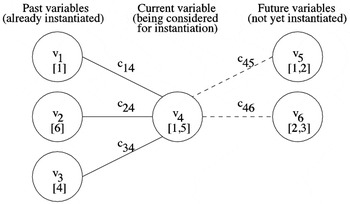
The acceptable-weight heuristic selects the value that minimizes the absolute difference between sw(S′′) and IdealSW′′. The following example will illustrate the typical situation. Figure 2 shows the relevant subproblem, consisting of variables v1,…,v4 and constraints c14, c24, and c34. Current domains are shown in square brackets under each variable name. Two future variables with constraints involving v4 are depicted in the diagram but are not considered by the heuristic.

An illustration of the acceptable-weight heuristic. The domain values and weights (in italics) for the subproblem considered by the heuristic are v1 = {1 = 0.1}, v2 = {6 = 0.2}, v3 = {4 = 0.4}, and v4 = {1 = 0.4, 5 = 0.8}. The relevant constraint tuples and their weights (in italics) are c14 = {(1, 1) = 0.1, (1, 5) = 0.2}, c24 = {(6, 1) = 0.8, (6, 5) = 0.9}, and c34 = {(4, 1) = 0.6, (4, 5) = 0.7}. See the text for further details.
In this example, search is at the point of instantiating v4. The possible values are 1 (whose weight is 0.4) and 5 (whose weight is 0.8), and the acceptable-weight heuristic is supposed to suggest one of them. Let us take a look at the implications of selecting each value, assuming that AIW = 0.4 at this point in the search.
In this example V′′ = {v1,v2,v3,v4}, and C′′ = {c14, c24, c34}. If we choose to assign 1 to v4, then sw(S′′) = (0.1 + 0.2 + 0.4) + 0.4 + (0.1 + 0.8 + 0.6) = 2.6. If we choose 5, then sw(S′′) = (0.1 + 0.2 + 0.4) + 0.8 + (0.2 + 0.9 + 0.7) = 3.3. After computing IdealSW′′ = (0.1 + 0.2 + 0.4) + AIW + 3·AIW = 2.3, we see that selecting the value 1 will yield a weight for S′′ that is closer to IdealSW′′. After the assignment of v4, acceptable-weight recomputes the AIW, to compensate for the amount we were off.
The strategy behind the heuristic described is twofold. Locally, we try to make sure that each small subproblem centered around the current variable has a weight that is in line with the global IdealSW. Globally, by constantly adjusting the AIW we try to control the overall deviation of the solution weight. Note that the algorithm is still complete; if search backs up due to failure, the acceptable-weight heuristic finds the value with the best weight from among the remaining values in a domain. This strategy appears to work well in practice, as we will see in Section 6.
5. INTERPRETATION AND USE OF SOLUTION WEIGHTS
Clearly, the solution weights as used in this paper cannot be taken to represent preferences directly, because typically we do not search for solutions with the maximum weight. They can be related to preferences by considering distances between a given solution weight and the ideal weight; the greater this distance, the lower the preference. This kind of interpretation has considerable psychological support, at least for simple sensory dimensions (Coombs & Avrunin, 1977).
Because a solution weight is the sum of many individual weights, one interpretation of it is as a summary quality, for example price. When we use the acceptable-weight heuristic, we are trying to focus on one subrange of values for this quantity. In terms of our criterion for acceptance, we are making a “strong homogeneity assumption,” that any combination of weights yielding a given sum is equally acceptable. Note that the heuristic itself will bias sampling from this set in favor of solutions with individual weights closer to the average. However, this is still consistent with our assumption because any solution within this set is equally acceptable.
As already noted, a potentially important application of this approach is “upselling,” in which we start from a given product or configuration and search for related systems that are higher in price. We do not necessarily know which combination of new values will be most satisfactory, but we want to narrow the search to those having a certain difference in price from the original entity.
The idea of preferable distance can be extended to other global measures, such as complexity or simply magnitude (larger, and/or faster, and/or greater capacity, etc.). In addition, in these cases as well as for price, we can either focus on some a priori ideal point or search for a possible ideal point that the user might already have.
The acceptable-weight heuristic is nicely suited to these kinds of tasks, because it allows one to choose a given weight as an ideal, which it then zeros in on. Because it takes a heuristic approach, it has the potential to find solutions quickly (cf. next section), in contrast to more laborious optimization procedures like branch and bound for MAX-CSPs (Jampel et al., 1996).
In these cases, derivation of weights for domain values can be done automatically by considering the difference between a value that serves as the origin point and the present value for that variable. The initial solution may be obtained by the customer through an interactive strategy, such as constraint-based matchmaking (Freuder & Wallace, 2002). Alternatively, an “original” solution can be chosen by the system on an a priori basis. Constraint weights can be derived in accordance with the value weights, that is, to maximize the likelihood that values with the appropriate weights will be chosen. Users can influence this process directly by specifying ideal values for certain variables or variable combinations; or they can simply characterize an ideal solution, for example, in terms of a difference in price, from which individual weights can be derived.
6. EXPERIMENTAL RESULTS
The acceptable-weight heuristic has been tested successfully on a small PC-configuration model (built according to specifications provided by Concentra, Inc., now part of Oracle, Inc.). However, in order to evaluate its performance more systematically we performed experimental tests on problems that were randomly generated (random CSPs). This allowed us to test the ability of this heuristic to find solutions in weight ranges with diminishing numbers of solutions.
Problems were generated using a probability of inclusion model with fixed numbers of elements. Under the probability of inclusion model, any element of each type (constraints, domain values, or constraint tuples) is included in the problem with a stipulated probability; in the fixed version, in addition, the whole process is repeated until the number of elements actually chosen is the same as the expected number of such elements given this probability. For example, if there is a constraint between two variables, both with domains of size 4, and the stipulated probability of inclusion of a constraint tuple is 0.75, each of the possible 16 tuples is considered for inclusion using a probability of 0.75 and the process is repeated (each time from scratch) until the number of tuples in the constraint is 12. For each value and constraint tuple, a weight was also chosen at random within the range [0,1].
For the present tests we used the maintained arc consistency (MAC) algorithm (Sabin & Freuder, 1994). This algorithm is a form of backtrack search, where search is interleaved with consistency maintenance among the domains of variables that are not yet instantiated. Specifically, after each selection of a variable and a value for assignment, the domains of all the uninstantiated variables are made pairwise consistent, or “arc consistent” (Mackworth, 1977). This means that for any pair of variables linked by a constraint, each value in one of the domains is supported by at least one value in the other domain (hence the name maintained arc consistency). This algorithm is part of a constraint satisfaction library developed at the University of New Hampshire, which is freely available at http://www.hulubei.net/tudor/csp.
Our tests compared the performance of MAC+acceptable-weight with that of MAC. In both cases we used a standard arc consistency algorithm known as AC-3 and the dynamic minimal domain size variable-ordering heuristic. The algorithms were used to find acceptable solutions to problems with 100 variables, each variable having five values in its domain. All the instances we tested had very similar behavior, and we chose one of them to show in each of the experiments presented here. The reason for showing just one problem instance in Figures 3, 4, 5, 6, and 7 is that we were interested in comparing different intervals of acceptable weights for each problem.
The constraint density (defined as the fraction of the possible constraints, beyond the minimum n − 1, that the problem has) and the constraint tightness (defined as the fraction of all possible pairs of values from the domains of two variables that are not allowed by a constraint) were used to vary the difficulty of the generated problems in order to study changes in the behavior of acceptable-weight. In the following tests we will compare the time required by the two algorithms to find an acceptable solution. Both algorithms will look for solutions in ranges of a given size (0.05 and 0.1 in the examples below) centered around the solution weight on the X axis, which has been translated and scaled from [MinSW(Pw), MaxSW(Pw)] to [0,1] . We set a timeout limit at 6 s, because we were interested in the performance of algorithms that could be used in an interactive setting, as well as algorithms that could find a series of solutions close to a desired weight in a short time period.
Before going any further, we need to briefly explain the behavior of MAC on these problems. Without going into details, we will just say that, probabilistically speaking, there are many solutions with weights around 0.5 and very few solutions with extreme weights (close to 0 or 1). MAC does not take weights into account, and thus from its point of view the solutions are distributed throughout the search space. However, as most solutions have weights around 0.5, MAC will tend to find those pretty quickly.
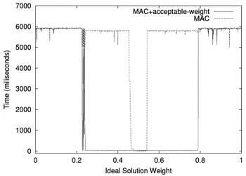
The first test we did was with density = 0 and tightness = 0. Figure 3 shows the performance difference between the two algorithms. Whereas MAC can only find solutions with weights in the 0.455–0.54 range, MAC+acceptable-weight is capable of finding solutions with weights in the 0.226–0.79 range. Moreover, in most cases the very first solution that MAC+acceptable-weight finds is within the acceptable range.

The behavior of MAC and MAC+acceptable-weight on a single test problem as described in the text. The solution weights are normalized to fall between 0 and 1. The range of acceptable weights is 0.05, which is centered at varying points along the scale of solution weights. The problems have a density of 0 (n − 1 edges) and a tightness of 0, so there are many solutions.
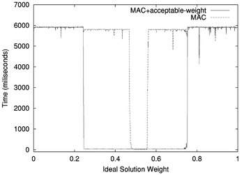
The test in Figure 4 was similar to the one in Figure 3 except that the constraint tightness was increased to 0.25. As a result, the range in which MAC+acceptable-weight can find acceptable solutions decreases slightly to 0.244–0.752. The range in which MAC finds acceptable solutions also changes a little, to 0.469–0.560.

A performance comparison of MAC and MAC+acceptable-weight with a weight range of 0.05 for a problem with a density of 0 and a tightness of 0.25. (Increased tightness reduces the number of possible solutions.)
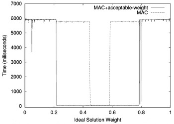
The first two results presented were performed with a range 0.05 size. That is, any solution with a weight that differs in absolute value by at most 0.025 from the ideal weight was considered acceptable. As we widen the acceptable range, the interval in which both algorithms quickly find solutions widens. In the test pictured in Figure 5, MAC was capable of finding acceptable solutions with weights in the 0.444–0.584 range. MAC+acceptable-weight performed much better, covering the 0.216–0.798 range. (Also note that this improves on the 0.244–0.752 range in Fig. 4.)

A performance comparison of MAC and MAC+acceptable-weight with a weight range of 0.1 for a problem with a density of 0 and a tightness of 0.25.
In our fourth test we increased the constraint graph density while keeping the tightness at 0.25 and the range at 0.1. In this test (Fig. 6), MAC alone covered the 0.447–0.569 range whereas MAC+acceptable-weight covered 0.415–0.568. (The spike around 0.601 marks a small region where MAC+acceptable-weight found acceptable solutions; with a longer time limit it would have covered the 0.568–0.601 range as well.)

A performance comparison of MAC and MAC+acceptable-weight with a weight range of 0.1 for a problem with a density of 0.055 and a tightness of 0.25.
Thus, as the problems get harder, the impact of acceptable-weight becomes less noticeable. In terms of weights, the density of solutions is given by a normal distribution. The reason for the performance degradation is that as density and/or tightness increase, the number of solutions decreases and the areas affected the most are those at the sides of the normal distribution curve, which contain a very small number of solutions to begin with. Gradually, the range covered by MAC+acceptable-weight will shrink to a range comparable to that covered by MAC alone (Fig. 6), because there will be virtually no solutions out- side a small range around 0.5 and MAC will be able to find those equally fast just by looking for any solution.
For the problems tested here (100 variables, domain size 5), the difficulty peak (Cheeseman et al., 1991) for a tightness of 0.25 is around a density of 0.0651 (Fig. 8). Around this peak MAC+acceptable-weight still compares well with MAC (Fig. 7). It should be noted, however, that we are not targeting hard problems with this heuristic. As stated earlier, configuration problems are often relatively easy, so there are lots of solutions; the challenge is to find one that is acceptable.

A performance comparison of MAC and MAC+acceptable-weight with a weight range of 0.1 for a problem in the “hard” region of the density space (density = 0.0651, tightness = 0.25).

A graph showing the transition between solvable and unsolvable problems as the density of the constraint graph increases. The time is that required to find one solution (in any part of the search space). The peak difficulty for search is at the boundary, or phase transition, between solvable and unsolvable problems. All problems have a tightness of 0.25.
These experiments show that the acceptable-weight heuristic is able to find solutions even if there are relatively few candidates, in contrast to ordinary CSP algorithms. The speed with which solutions were found (generally under 1 s) for problems of this size supports the contention that this heuristic approach will often outperform optimization-based approaches (cf. Jampel et al., 1996). Because there was typically a very sharp transition between the region where problems were found quickly and regions where locating problems was quite difficult, it is clear that similar results would be found even if the cutoff time was reduced to as little as 1 s.
7. FUTURE WORK
One way to improve the performance of the heuristic might be by trying to detect situations where search gets stuck in a given range. There are situations where MAC+acceptable-weight obtains a partial solution, but there is no way of extending it to a complete solution with an acceptable weight. It is clear that in those situations the heuristic has made a few mistakes, and it might be interesting to see if the overall performance can be improved by refusing to listen to the heuristic's suggestions until the range of solution weights that are obtained changes. Somewhat related ideas can be found in Harvey and Ginsberg (1995).
Another idea would be to avoid searching in subtrees where there is no way of extending the current partial solution to a complete solution with an acceptable weight. Rough estimates of the potential contribution of the unsolved part of the problem can be obtained by computing its minimum and maximum solution weights (MinSW and MaxSW). In addition, we may be able to obtain better weight evaluations for the small subproblems centered around the current variable. In particular, we would like to be able to take future variables into account in this process.
Another reasonable extension is to conditional or dynamic CSPs, where the inclusion of variables or constraints in a problem may depend on prior instantiations, especially because this variant of the constraint satisfaction problem was developed for use with configuration problems (Mittal & Falkenhainer, 1990). Because the acceptable-weight heuristic uses a moving average, it should be possible to adapt it to problems that change dynamically. At the same time, this is another case where it would be useful to be able to take future variables into account when calculating weight evaluations during search.
8. CONCLUSIONS
Goldilocks learned a very important lesson. There are things in life that are not the right size for everyone. It is often the case that there is a wide range of choices to pick from and we have to determine which one is too big, too small, or just right. Worse still, we sometimes have to relax our notion of just right to get something that is good enough. One of the most exciting trends in product configuration involves the application of this lesson to product development, under the banner of “mass customization” (Felfernig et al., 2001).
The acceptable-weight heuristic presented here has obvious relevance for this effort, because it is designed to guide the search toward solutions with acceptable weights, when solutions can be ranked along a given dimension. Although we believe there are avenues for improvement, our experiments have shown that this heuristic, combined with MAC, can find acceptable solutions very quickly across a fairly wide range of target values.
ACKNOWLEDGMENTS
This material is based on work supported by Oracle Corporation and by the National Science Foundation under Grant IRI-9504316 and carried out while the authors were in the Department of Computer Science at the University of New Hampshire. Work on the paper was supported in part by Science Foundation Ireland under Grant 00/PI.1/C075. The second author is currently supported by a Principal Investigator Award from Science Foundation Ireland. Several parts of this paper were improved by the comments of the anonymous reviewers.
References
REFERENCES
Cheeseman, P.,
Kanefsky, B., &
Taylor, W.
(1991).
Where the really hard problems are.
Proc. Twelfth Int. Joint Conf. Artificial Intelligence, pp.
331–337.
San Mateo, CA:
Morgan Kaufmann.
Coombs, C. &
Avrunin, G.
(1977).
Single-peaked functions and the theory of preference.
Psychological Review
84(2),
216–230.CrossRefGoogle Scholar
Felfernig, G.,
Friedrich, G., &
Jannach, D.
(2001).
Conceptual modeling for configuration of mass-customizable products.
Artificial Intelligence in Engineering
15(2),
165–176.Google Scholar
Freuder, E. &
Wallace, R.
(2002).
Suggestion strategies for constraint-based matchmaker agents.
International Journal on Artificial Intelligence Tools
11(1),
3–18.Google Scholar
Harvey, W. &
Ginsberg, M.
(1995).
Limited discrepancy search.
Proc. Fourteenth Int. Joint Conf. Artificial Intelligence, pp.
607–613.
San Mateo, CA:
Morgan Kaufmann.
Hulubei, T. &
Freuder, E.
(1999).
The Goldilocks problem. In
Principles and Practice of Constraint Programming—CP'99, Lecture Notes in Computer Science, No. 1713
(Jaffar, J., Ed.), pp.
234–245.
Berlin:
Springer.
Jampel, M.,
Freuder, E., &
Maher, M. (Eds.).
(1996).
Over-Constrained Systems. Selected Papers From the Workshop on
Over-Constrained Systems—CP '95.
Lecture Notes in Computer Science, No. 1106.
Berlin:
Springer.CrossRef
Mackworth, A.
(1977).
Consistency in networks of relations.
Artificial Intelligence
8,
99–118.Google Scholar
Mittal, S. &
Falkenhainer, B.
(1990).
Dynamic constraint satisfaction problems.
Proc. Eighth National Conf. Artificial Intelligence, pp.
25–32.
Menlo Park, CA:
AAAI Press.
Mittal, S. &
Frayman, F.
(1989).
Towards a generic model of configuration tasks.
Proc. Eleventh Int. Joint Conf. Artificial Intelligence, pp.
1395–1401.
San Mateo, CA:
Morgan Kaufmann.
Sabin, D. &
Freuder, E.
(1994).
Contradicting conventional wisdom in constraint satisfaction.
Proc. Eleventh Eur. Conf. Artificial Intelligence
(Cohn, A., Ed.), pp.
125–129.
Chichester, UK:
Wiley.
Sabin, D. &
Weigel, R.
(1998).
Production configuration frameworks—A survey.
IEEE Intelligent Systems
13(4),
42–49.CrossRefGoogle Scholar
Wielinga, B. &
Schreiber, A.
(1997).
Configuration design problem solving.
IEEE Expert
12(2),
49–56.CrossRefGoogle Scholar

An example problem. For variables v1, v2, and v3, the values and weights (in italics) are v1 = {0 = 0.2, 1 = 0.8}, v2 = {1 = 0.1, 2 = 0.7}, and v3 = {−1 = 0.8, 4 = 0.9}. For c12, the constraint between v1 and v2, individual tuples and weights (in italics) are {(0, 1) = 0.1, (1, 1) = 0.7, (1, 2) = 0.9}. For c13 they are {(0, −1) = 0.2, (0, 4) = 0.3, (1, −1) = 0.5}.
An illustration of the acceptable-weight heuristic. The domain values and weights (in italics) for the subproblem considered by the heuristic are v1 = {1 = 0.1}, v2 = {6 = 0.2}, v3 = {4 = 0.4}, and v4 = {1 = 0.4, 5 = 0.8}. The relevant constraint tuples and their weights (in italics) are c14 = {(1, 1) = 0.1, (1, 5) = 0.2}, c24 = {(6, 1) = 0.8, (6, 5) = 0.9}, and c34 = {(4, 1) = 0.6, (4, 5) = 0.7}. See the text for further details.
The behavior of MAC and MAC+acceptable-weight on a single test problem as described in the text. The solution weights are normalized to fall between 0 and 1. The range of acceptable weights is 0.05, which is centered at varying points along the scale of solution weights. The problems have a density of 0 (n − 1 edges) and a tightness of 0, so there are many solutions.
A performance comparison of MAC and MAC+acceptable-weight with a weight range of 0.05 for a problem with a density of 0 and a tightness of 0.25. (Increased tightness reduces the number of possible solutions.)
A performance comparison of MAC and MAC+acceptable-weight with a weight range of 0.1 for a problem with a density of 0 and a tightness of 0.25.
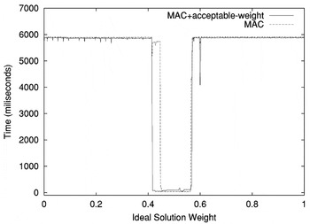
A performance comparison of MAC and MAC+acceptable-weight with a weight range of 0.1 for a problem with a density of 0.055 and a tightness of 0.25.
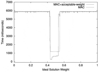
A performance comparison of MAC and MAC+acceptable-weight with a weight range of 0.1 for a problem in the “hard” region of the density space (density = 0.0651, tightness = 0.25).
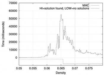
A graph showing the transition between solvable and unsolvable problems as the density of the constraint graph increases. The time is that required to find one solution (in any part of the search space). The peak difficulty for search is at the boundary, or phase transition, between solvable and unsolvable problems. All problems have a tightness of 0.25.
 You have
Access
- 5
- Cited by