



1. Introduction
Axisymmetric configurations are frequently employed in supersonic aerodynamics to eliminate three-dimensional and highly nonlinear effects that complicate the interpretation of experimental and theoretical results. Early experiments concerning Mach-5.3 flow over a hollow cylinder/flare by Ginoux (Reference Ginoux1971) observed spanwise variations in skin friction in the reattachment region. Similarly, Benay et al. (Reference Benay, Chanetz, Mangin, Vandomme and Perraud2006) considered Mach-5 flow over a hollow cylinder/flare experimentally. Their results also revealed periodic but steady streamwise streaks in the reattachment region. Navier–Stokes simulations showed that experimental heat-flux values where 2.5 times larger than calculated laminar ones, therefore indicating a transitional shear layer. More recently, experiments were carried out by Lugrin et al. (Reference Lugrin, Nicolas, Severac, Tobeli, Beneddine, Garnier, Esquieu and Bur2022), again at Mach 5. They also reported streamwise streaks near reattachment, together with oblique modes travelling inside the shear layer.
Modern numerical research has aimed at explaining the origin of these streaks through high-fidelity simulations and stability calculations. The three-dimensional simulations of Brown et al. (Reference Brown, Boyce, Mudford and O'Byrne2009) showed that unforced steady-state axisymmetric flow becomes unsteady for Reynolds numbers larger than a critical value. Lugrin et al. (Reference Lugrin, Beneddine, Leclercq, Garnier and Bur2021) performed high-fidelity simulations of a hollow cylinder/flare at Mach 5 with random forcing and showed that oblique first modes were the cause of streaks at reattachment. Li & Hao (Reference Li and Hao2023) carried out both simulations and global stability analysis for supersonic flow over a hollow cylinder/flare at Mach number 2.25. Their former global stability criterion formulated for two-dimensional flow (Hao et al. Reference Hao, Cao, Wen and Olivier2021) was extended to the axisymmetric case.
This study follows our earlier paper (Exposito, Gai & Neely Reference Exposito, Gai and Neely2021) of the analysis of supersonic boundary layer separation over a compression corner. The boundary layer theory is one of the most powerful predictive frameworks with which to extract meaningful information from complex flow phenomena. The modern version of the boundary layer theory, namely ‘interactive boundary layer theory’ or ‘triple-deck theory’, considers the effect of the boundary layer growth on the inviscid, external flow. It was independently developed by Stewartson & Williams (Reference Stewartson and Williams1969) and Neiland (Reference Neiland1969). The boundary layer is split into three ‘decks’, based on the similarity parameter  $\varepsilon = Re^{-1/8}$, where
 $Re$ is the characteristic Reynolds number. In the lower deck, of height
 $O(\varepsilon ^5)$, the flow is viscous and incompressible; in the middle deck, of height
 $O(\varepsilon ^4)$, it is inviscid and rotational; and in the top deck, of height
 $O(\varepsilon ^3)$, it is inviscid and irrotational. The relationship between boundary layer growth and pressure is determined by the ‘interaction law’. Different configurations and flow conditions can be studied by changing the interaction law. This includes subsonic flow (Messiter Reference Messiter1970; Stewartson Reference Stewartson1970), supersonic flow (Werle & Vatsa Reference Werle and Vatsa1974; Rizzetta, Burggraf & Jenson Reference Rizzetta, Burggraf and Jenson1978; Smith Reference Smith1988; Smith & Khorrami Reference Smith and Khorrami1991; Cassel, Ruban & Walker Reference Cassel, Ruban and Walker1995) and hypersonic flow with wall cooling (Brown, Stewartson & Williams Reference Brown, Stewartson and Williams1975; Kerimbekov, Ruban & Walker Reference Kerimbekov, Ruban and Walker1994).
The application of the triple-deck theory to axisymmetric, supersonic flow becomes significantly simpler than its application to the general three-dimensional problem, due to symmetry. The interaction law for axisymmetric, supersonic flow was proposed by Kluwick, Gittler & Bodonyi (Reference Kluwick, Gittler and Bodonyi1984) based on the axisymmetric wave equation of Lighthill (Reference Lighthill1945) and Ward (Reference Ward1948):
 \begin{equation} p ={-} \frac{\partial a}{\partial x} + \frac{1}{R} \int_{-\infty}^x W \left( \frac{x - \xi}{R} \right) \frac{\partial a}{\partial \xi } {\rm d} \xi, \end{equation}
as expressed by Gittler & Kluwick (Reference Gittler and Kluwick1987). Here,  $a(x,t)$ is the net displacement function of the boundary layer;
 $R$ is the scale external radius of the axisymmetric body, which is assumed to be significantly larger than the boundary layer height (
 $\delta / R \ll 1$); and
 $W(\gamma )$ is the Ward function
 \begin{equation} W(\gamma) = \int_0^{\infty} \frac{{\rm e}^{-\lambda \gamma}}{K_1^2(\lambda) + {\rm \pi}^2 I_1^2(\lambda) } \frac{{\rm d} \lambda}{\lambda}, \end{equation}
where  $K_1$ and
 $I_1$ are Bessel functions, and
 $\lambda$ is the integration variable.
Figure 1 shows the triple-deck structure of the interaction region for an axisymmetric compression corner. Historically, the development of the axisymmetric supersonic triple-deck theory has closely followed that of the two-dimensional flow. Consider, for example, the free-interaction problem. In this case, a pressure perturbation is added to the Blasius boundary layer that develops over a flat plate. The evolution of the boundary layer is studied by solving triple-deck equations. The solution for the two-dimensional case was first obtained by Stewartson & Williams (Reference Stewartson and Williams1969), using a streamwise marching method. When reversed flow was obtained as a consequence of separation, the numerical algorithm was no longer suitable to solve this problem. The approximation of Reyhner & Flügge-Lotz (Reference Reyhner and Flügge-Lotz1968), which neglects the convective term in regions of reverse flow, was applied by Williams (Reference Williams1975) to extend the solution downstream of separation. A constant pressure plateau of 1.8 (in triple-deck scaling) was obtained downstream for the flat plate. The axisymmetric compressive free-interaction problem was considered by Kluwick, Gittler & Bodonyi (Reference Kluwick, Gittler and Bodonyi1985). In their study, the approximation of Reyhner & Flügge-Lotz (Reference Reyhner and Flügge-Lotz1968) was also employed. They found that for an infinite external radius of an axisymmetric body, the pressure plateau was equivalent to that of the two-dimensional case. As the external radius decreases, the pressure plateau also decreases and asymptotically reaches a constant value (Kluwick et al. Reference Kluwick, Gittler and Bodonyi1985).
Triple-deck structure of the interaction region at an axisymmetric compression corner. Starred quantities are physical variables.

The triple-deck theory was then employed to describe separated flow over a compression ramp with  $\alpha ^* > 0$, where
 $\alpha ^*$ is the geometric angle of the corner. For the two-dimensional problem, supersonic flow over a compression corner was considered by Stewartson (Reference Stewartson1970) using linearised theory, and by Ruban (Reference Ruban1978) and Rizzetta et al. (Reference Rizzetta, Burggraf and Jenson1978) using finite differences. Kluwick et al. (Reference Kluwick, Gittler and Bodonyi1984) considered both the linear and nonlinear version for the axisymmetric case. Compared with the two-dimensional case, the asymptotic pressure downstream of an axisymmetric compression corner of angle
 $\alpha$ is
 $p \sim {\alpha R}/{x}$, where
 $x$ is the streamwise coordinate and
 $\alpha$ is the scale angle. The pressure downstream of the ramp asymptotically tends to 0 as a consequence of the expansion of the streamtube area downstream of the corner, a phenomenon named ‘over-expansion’ (Gittler & Kluwick Reference Gittler and Kluwick1987). The shear-stress distribution was found to recover its flat plate value asymptotically far downstream of the corner. As the external radius is reduced, both pressure and shear-stress values at the corner decrease; and as the external radius is increased, pressure and shear-stress tend towards constant values similar to the two-dimensional case. Using the spectral method of Burggraf & Duck (Reference Burggraf and Duck1982), shear-stress and pressure distributions were obtained for scale angles up to 5 for several values of external radius. Incipient separation was found to occur at
 $\alpha \approx 3.39$. In their subsequent paper (Gittler & Kluwick Reference Gittler and Kluwick1987), pressure and shear-stress distributions for scale angles up to 9 were obtained. They solved the axisymmetric, supersonic triple-deck equations using both finite-differences and spectral methods. Again, the approximation of Reyhner & Flügge-Lotz (Reference Reyhner and Flügge-Lotz1968) was used to eliminate the convective term. Secondary separation was not observed for scale angles up to 9. To our knowledge, there has not been another study since of axisymmetric, supersonic flow separation over a compression corner using triple-deck theory. Despite significant advances both in fluid dynamic theory and computational power, important flow phenomena such as secondary separation and unsteadiness in separated axisymmetric supersonic flows have not been discussed within the framework of triple-deck theory to date. Our aim was to extend and improve upon the results of Gittler & Kluwick (Reference Gittler and Kluwick1987), who used the steady form of the triple-deck equations. However, we unexpectedly found a wave packet similar to that reported by Cassel et al. (Reference Cassel, Ruban and Walker1995) for two-dimensional flow. The present paper contains our analysis and discussion of this feature.
2. Governing equations
The unsteady triple-deck equations for supersonic flow over an axisymmetric compression corner are the continuity and momentum equations for incompressible flow in the lower deck:
 \begin{gather} \frac{\partial{u}}{\partial{x}} + \frac{\partial{v}}{\partial{y}} = 0, \end{gather}
 \begin{gather}\frac{\partial{u}}{\partial{t}} + u \frac{\partial{u}}{\partial{x}} + v \frac{\partial{u}}{\partial{y}} ={-} \frac{\partial{p}}{\partial{x}} + \frac{\partial^2 u}{\partial y^2}, \end{gather}
and the interaction law (1.1). All variables are scaled using triple-deck scalings, which are given by Gittler & Kluwick (Reference Gittler and Kluwick1987),
 \begin{gather} x = C^{{-}3/8} \lambda^{5/4} |M_{\infty}^2 - 1|^{3/8} \left( \frac{T_w^*}{T^*_{\infty}} \right)^{{-}3/2} \frac{x^* - L^*}{\varepsilon^3 L^*}, \end{gather}
 \begin{gather}y = C^{{-}5/8} \lambda^{3/4} |M^2_{\infty} - 1|^{1/8} \left( \frac{T^*_w}{T^*_{\infty}} \right)^{{-}3/2} \frac{ r^* - R^*}{\varepsilon^5 L^*} - f(x), \end{gather}
 \begin{gather}p = C^{{-}1/4} \lambda^{{-}1/2} |M^2_{\infty} - 1|^{1/4} \frac{p^* - p^*_{\infty} }{\varepsilon^2 \rho^*_{\infty} u^*_{\infty}}, \end{gather}
 \begin{gather}u = C^{{-}1/8} \lambda^{{-}1/4} |M^2_{\infty} - 1|^{1/8} \left( \frac{T_w^*}{T^*_{\infty}} \right)^{{-}1/2} \frac{u^*}{\varepsilon u^*_{\infty}}, \end{gather}
 \begin{gather}v = C^{{-}3/8} \lambda^{{-}3/4} |M^2_{\infty} - 1|^{{-}1/8} \left( \frac{T^*_{w}}{T^*_{\infty}} \right)^{{-}1/2} \frac{v^*}{\varepsilon^3 u^*_{\infty}}, \end{gather}
 \begin{gather}a = C^{{-}5/8} \lambda^{3/4} |M^2_{\infty} - 1|^{1/8} \left( \frac{T^*_w}{T^*_{\infty}} \right)^{{-}3/2} \frac{a^*}{\varepsilon^5 L^*}, \end{gather}
 \begin{gather}R = C^{{-}3/8} \lambda^{5/4} |M^2_{\infty} -1 |^{7/8} \left( \frac{T^*_w}{T^*_{\infty}} \right)^{{-}3/2} \frac{R^*}{\varepsilon^3 L^*}. \end{gather}
Here,  $C$ is the Chapman constant,
 $\lambda$ the Blasius constant,
 $M$ the Mach number,
 $T^*_w$ the wall temperature,
 $T^*_{\infty }$ the free stream temperature,
 $x^*$ the longitudinal coordinate,
 $L^*$ the flat-plate length,
 $r^*$ the radial coordinate,
 $R^*$ the external radius,
 $f(x)$ the surface shape,
 $p^*$ the pressure,
 $\rho ^*$ the density,
 $T^*$ the temperature,
 $u^*$ the longitudinal velocity,
 $v^*$ the radial velocity and
 $a^*$ the displacement thickness, with the asterisk indicating dimensional quantities.
In our computations, the interaction law is expressed in terms of the total displacement function,  $A(x,t) = a(x,t) + f(x)$. It is obtained from the boundary condition
 \begin{equation} u \rightarrow y + A \quad \textrm{as}\ y \rightarrow \infty. \end{equation}
At the wall, the usual no-slip boundary conditions apply,
 \begin{equation} u = v = 0, \quad \textrm{at}\ y = 0. \end{equation}
The boundary conditions upstream of the corner are equivalent to those of the two-dimensional case,
 \begin{gather} u \rightarrow y \quad \textrm{as}\ x \rightarrow -\infty, \end{gather}
 \begin{gather}p \rightarrow 0 \quad \textrm{as}\ x \rightarrow -\infty. \end{gather}
Using the shear stress  $\tau = \partial u / \partial y$, the following boundary condition downstream of the corner applies:
 \begin{equation} \tau_w = 1 - \frac{2 \alpha R Ai(0)}{3 Ai'(0) \varGamma\left(\dfrac{1}{3} \right) x^{5/3} } \left[ \ln \frac{x}{R} - \phi \left( - \frac{5}{3} \right) \right], \end{equation}
where  $Ai(z)$ is the Airy function and
 $\phi (z)$ is the digamma function (Kluwick et al. Reference Kluwick, Gittler and Bodonyi1984). For large values of
 $x$, this expression is equivalent to the boundary condition
 $\tau \rightarrow 1$.
The following boundary condition applies downstream of the domain (Gittler & Kluwick Reference Gittler and Kluwick1987):
 \begin{equation} p \rightarrow \alpha \left[ \frac{R}{x} + 2 \frac{R^3}{x^3} \ln \frac{x}{R} + O \left( \frac{R^3}{x^3} \right) \right] \quad \textrm{as}\ x \rightarrow \infty; \end{equation}
therefore, pressure decreases following a hyperbolic curve at the downstream end of the domain.
3. Asymptotic limits of the interaction law
Before proceeding with nonlinear simulations, it is instructive to explore the behaviour of the interaction in the limits of large ( $R \gg 1$) and small (
 $R \ll 1$) scale external radius. The Ward function is a fast decaying function, as shown in figure 2. The largest values are obtained for arguments
 $\gamma$ close to
 $\gamma = 0$, while for
 $\gamma \gg 1$, the function rapidly decreases to zero. Considering
 $\gamma = (x - \xi ) / R$, there is an interval of values
 $\xi$ for which the Ward function is of order one, and much smaller than one outside of this interval. For example, for
 $\xi = x$,
 $W(0)=0.5=O(1)$, and for
 $\xi = x - 10R$,
 $W(10)=0.01 \ll 1$. We therefore explore the interval
 $\xi \in [x - R^{k+1}, x]$, where
 $k$ is a constant,
 \begin{align} \frac{1}{R} \int_{-\infty}^x W \left( \frac{x - \xi}{R} \right) \frac{\partial a}{\partial \xi } {\rm d} \xi &= \frac{1}{R} \int_{-\infty}^{x-R^{k+1}} W \left( \frac{x - \xi}{R} \right) \frac{\partial a}{\partial \xi } {\rm d} \xi \nonumber\\ &\quad +\frac{1}{R} \int_{x-R^{k-1}}^x W \left( \frac{x - \xi}{R} \right) \frac{\partial a}{\partial \xi } {\rm d} \xi. \end{align}
Ward function for values of  $\gamma$ between 0 and 100.

It is assumed that the first term is negligible, whereas the second term can be simplified by evaluating the Ward function at the midpoint, thereby integrating the derivative
 \begin{equation} \frac{1}{R} \int_{x-R^{k-1}}^x W \left( \frac{x - \xi}{R} \right) \frac{\partial a}{\partial \xi } {\rm d} \xi \approx \frac{W(R^k / 2)}{R} \int_{x - R^{k+1}}^x \frac{\partial a}{\partial \xi} {\rm d} \xi = \frac{W(R^k / 2)}{R} [a|_{x} - a |_{x-R^{k+1}}]. \end{equation}
The interaction law (1.1) is then approximated as
 \begin{equation} p \approx{-} \frac{\partial a}{\partial x} + \frac{W(R^k / 2)}{R} [ a|_{x} - a|_{x-R^{k+1}}]. \end{equation}
To further simply this expression, we consider the Taylor expansion of the Ward function to order  $n_1$,
 \begin{equation} W(R^k / 2) \approx \sum_{k_1=0}^{n_1} \frac{R^{k_1k}}{2^{k_1}} \int_0^{\infty} \frac{ \dfrac{(-\lambda)^{k_1}}{k_1!} }{\lambda(K_1^2 + {\rm \pi}^2 I_1^2)} {\rm d} \lambda, \end{equation}
as well as that of the term  $a|_{x - R^{k+1}}$ to order
 $n_2$,
 \begin{equation} a|_{x - R^{k+1}} = a|_{x} + \left.\frac{\partial a}{\partial x}\right|_{x} ({-}R^{k+1} ) + \cdots \approx a|_{x} + \sum_{k_2=1}^{n_2} \frac{a^{(k_2)}}{k_2!} ({-}R^{k+1})^{k_2}. \end{equation}
The approximation of the pressure is
 \begin{equation} p \approx{-}\frac{\partial a}{\partial x} - \frac{1}{R} \left(\sum_{k_1=0}^{n_1} \frac{R^{k_1k}}{2^{k_1}} \int_0^{\infty} \frac{\dfrac{(-\lambda)^{k_1}}{k_1!} }{\lambda(K_1^2 + {\rm \pi}^2 I_1^2)} {\rm d} \lambda \right) \left(\sum_{k_2=1}^{n_2} \frac{a^{(k_2)}}{k_2!} ({-}1)^{k_2} R^{k_2(k+1)} \right) . \end{equation}
For a large radius  $R \gg 1$, the two-dimensional interaction
 $p = - \partial a / \partial x$ must be recovered. The largest exponent of
 $R$ must obey the following relationship:
 \begin{equation} {-}1 + n_1 k + n_2 (k+1) <0. \end{equation}
If both expansions  $n_1$ and
 $n_2$ are equal, it is found that the constant
 $k$ must be such that
 $k < - 1/2$ for the above relation to be valid. This is physically consistent, since for
 $k<0$,
 $\xi = x - R^k$ tends towards
 $x$ in the limit
 $R \rightarrow \infty$, which eliminates the integral from the interaction law, resulting in the two-dimensional interaction law. For the specific case
 $k = -1$, ignoring terms of order
 $O(R^{-2})$ in the expansion of the displacement function leads to the relation
 \begin{equation} p \approx{-} \frac{\partial a}{\partial x} \left( 1 - \frac{W(R^{{-}1}/2)}{R^2} \right) + O(R^{{-}2}), \end{equation}
which approaches the two-dimensional expression for  $R \gg 1$.
For the case  $R \ll 1$, the series (3.6) is convergent if the largest exponent obeys the opposite relation,
 \begin{equation} {-}1 + n_1 k + n_2 (k+1) >0. \end{equation}
Again, for the case of uniform expansions, it is easy to show that the relation is met for any non-negative value of  $k$. Selecting
 $k =0$ and neglecting terms of order
 $O(R^2)$, we have
 \begin{equation} p \approx{-} \frac{\partial a}{\partial x} \left( 1 - \frac{W(1/2)}{R} \right) + O(R^2) . \end{equation}
This relation is consistent with numerical results shown in the following sections, which indicate that a decrease in external radius leads to a more significant over-expansion effect, therefore reducing the pressure gradient induced by the corner. Note that in the case where  $R = W(1/2) = O(1)$, (3.10) does not hold.
4. Numerical method
4.1. General formulation
The Ruban–Cassel method (RCM) employs the shear stress formulation of the triple-deck equations. The momentum equation (2.1) is
 \begin{equation} \frac{\partial{\tau}}{\partial{t}} + u \frac{\partial{\tau}}{\partial{x}} + v \frac{\partial{\tau}}{\partial{y}} = \frac{\partial^2 \tau}{\partial y^2}. \end{equation}
Using the stream function  $u = \partial \psi / \partial y$,
 $v = - \partial \psi / \partial x$, the velocities are recovered from the shear stress solution with
 \begin{equation} \frac{\partial^2 \psi}{\partial y^2} = \tau. \end{equation}
The displacement function is expressed as
 \begin{equation} A(x,t) = \lim_{y\rightarrow \infty} (u - y) = \lim_{y \rightarrow \infty} \int_0^{y} (\tau - 1)\,{{\rm d}y}, \end{equation}
and the boundary conditions are
 \begin{equation} \tau \rightarrow 1 \quad \textrm{as}\ x \rightarrow \pm \infty. \end{equation}
Using the following relationship:
 \begin{equation} \frac{\partial{p}}{\partial{x}} = \left.\frac{\partial{\tau}}{\partial{y}}\right|_{y=0}, \end{equation}
the interaction law (1.1) is written as
 \begin{equation} \left.\frac{\partial{\tau}}{\partial{y}} \right|_{y = 0} ={-} \frac{\partial^2 A}{\partial x^2} + \frac{{\rm d}^2 f}{{{\rm d}\kern0.07em x}^2} + \frac{1}{R} \frac{\partial{}}{\partial{x}} \int_{-\infty}^x W \left(\frac{x - \xi}{R} \right) \left( \frac{\partial A}{\partial \xi} - \frac{{\rm d} f}{{\rm d} \xi} \right) {\rm d} \xi. \end{equation}
Rewriting (4.6) as
 \begin{equation} \tau^{(1)} = \tau^{(2)} + \tau^{(3)} + \tau^{(4)}, \end{equation}
where each term is
 \begin{gather} \tau^{(1)} =\left. \frac{\partial{\tau}}{\partial{y}} \right|_{y = 0}, \end{gather}
 \begin{gather}\tau^{(2)} ={-} \frac{\partial^2 A}{\partial x^2}, \end{gather}
 \begin{gather}\tau^{(3)} = \frac{{\rm d}^2 f}{{{\rm d}\kern0.07em x}^2}, \end{gather}
 \begin{gather}\tau^{(4)} = \frac{1}{R} \frac{\partial{}}{\partial{x}} \int_{-\infty}^x W \left( \frac{x - \xi}{R} \right) \left(\frac{\partial A}{\partial \xi} - \frac{{\rm d} f}{{\rm d} \xi} \right) {\rm d} \xi, \end{gather}
we can see that the terms  $\tau ^{(1)} = \tau ^{(2)} + \tau ^{(3)}$ were already discretised by Ruban (Reference Ruban1978) and Cassel et al. (Reference Cassel, Ruban and Walker1995). Our discretisation is equivalent to theirs. The initial condition corresponds to that of the lower part of a Blasius boundary layer,
 $u=y$. The solution is advanced in time at a constant time step
 $\Delta t$, with wall-normal derivatives evaluated implicitly. Streamwise and wall-normal velocities are evaluated at the former step via the streamfunction. The streamwise and wall-normal dimensions are divided into
 $I-1$ and
 $J-1$ elements of step sizes
 $\Delta x$ and
 $\Delta y$. Each mesh node is indicated by the subscripts
 $i$ and
 $j$, which correspond to the streamwise (
 $i = 1, \ldots, I$) and wall-normal (
 $\,j=1, \ldots, J$) dimensions, respectively. This formulation leads to a tridiagonal system of equations, which is solved with a Thomas algorithm that provides values
 $N_i$ and
 $M_i$. These coefficients are then employed to obtain wall shear-stress values with the interaction law. The reader is referred to the study of Cassel et al. (Reference Cassel, Ruban and Walker1995) for the exact expression of these coefficients.
4.2. Axisymmetric interaction law
Regarding  $\tau ^{(4)}$, we first apply the Leibniz rule
 \begin{align} \tau^{(4)} &= \frac{1}{R} \frac{\partial{}}{\partial{x}} \int_{-\infty}^x W \left(\frac{x - \xi}{R} \right) \left( \frac{\partial A}{\partial \xi} - \frac{{\rm d} f}{{\rm d} \xi} \right) {\rm d} \xi \nonumber\\ &= \frac{W(0)}{R} \left( \frac{\partial A}{\partial x} - \frac{{\rm d} f}{{\rm d}\kern0.07em x} \right) + \frac{1}{R} \int_{-\infty}^x \frac{{\rm d} }{{{\rm d}\kern0.07em x}} \left[ W \left( \frac{x - \xi}{R} \right) \left(\frac{\partial A}{\partial \xi} - \frac{{\rm d} f}{{\rm d} \xi} \right) \right] {\rm d} \xi. \end{align}
Equation (4.12) is split into the following terms:
 \begin{gather} \tau^{(4)}_A = \frac{W(0)}{R} \left( \frac{\partial A}{\partial x} - \frac{{\rm d} f}{{\rm d}\kern0.07em x} \right) , \end{gather}
 \begin{gather}\tau^{(4)}_B = \frac{1}{R} \int_{-\infty}^x \frac{{\rm d}}{{\rm d}\kern0.07em x} \left[ W \left( \frac{x - \xi}{R} \right) \frac{\partial A}{\partial \xi} \right] {\rm d}\xi, \end{gather}
 \begin{gather}\tau^{(4)}_C ={-} \frac{1}{R} \int_{-\infty}^x \frac{{\rm d}}{{\rm d}\kern0.07em x} \left[ W \left( \frac{x - \xi}{R} \right) \frac{{\rm d} f}{{\rm d} \xi} \right] {\rm d} \xi. \end{gather}
The derivatives of the Ward function are denoted by  $G(z) = {\rm d} W(z) / {\rm d} z$ and
 $D(z) = {\rm d}^2 W(z) / {\rm d} z^2$, where
 $z = (x - \xi ) / R$. These are known and can be calculated with a Gauss–Laguerre formula.
Consider streamwise station  $x_i$. As described by Cassel et al. (Reference Cassel, Ruban and Walker1995), the discretisation of the displacement function at this station can be obtained with the wall-shear stress at station
 $i$,
 \begin{equation} \int_0^{y_{max}} (\tau - 1) \,{{\rm d}y} = N_i \tau_{i,1} + M_i, \end{equation}
where  $y_{max}$ is the domain height. Applying second-order differences, the value of
 $\tau _A^{(4)}$ at
 $x_i$ is
 \begin{equation} \tau^{(4)}_{A,i} = \frac{W(0)}{R} \left[ \left( \frac{N_{i+1} \tau_{i+1,1} - N_{i-1,1} \tau_{i-1,1}}{2 \Delta x} + \frac{M_{i+1} - M_{i-1} }{2 \Delta x} \right) - \left.\frac{{\rm d} f}{{\rm d}\kern0.07em x}\right|_i \right]. \end{equation}
The term  $\tau _B^{(4)}$ is solved using integration by parts and the trapezoidal rule
 \begin{align} \tau_{B,i}^{(4)} &= \frac{1}{R^2} G(0) (N_i \tau_{i,1} + M_i) + \frac{\Delta x}{2 R^3} \sum_{k=2}^i \left[ (N_k \tau_{k,1} + M_k) D \left( \frac{x_i - x_k}{R} \right) \right.\nonumber\\ &\quad +\left. (N_{k-1} \tau_{k-1, 1} + M_{k-1}) D \left( \frac{x_i - x_{k-1}}{R} \right) \right]. \end{align}
Note that (4.16) turns the tridiagonal matrix of Ruban (Reference Ruban1978) at the wall into a lower triangular matrix, together with the diagonal corresponding to  $i+1$. The term
 $\tau _C^{(4)}$ is also approximated with the trapezoidal rule
 \begin{equation} \tau_{C,i}^{(4)} ={-} \frac{\Delta x}{2 R^2} \sum_{k=2}^{i} \left[ G \left( \frac{x_i - x_k}{R} \right) \left.\frac{{\rm d} f}{{\rm d}\kern0.07em x}\right|_k + G \left( \frac{x_i - x_{k-1}}{R} \right) \left.\frac{{\rm d} f}{{\rm d}\kern0.07em x}\right|_{k-1} \right]. \end{equation}
Considering the approximations of the two-dimensional case, (4.6) is finally expressed as
 \begin{equation} \sum_{k=1}^i \tilde{c}_k \tau_k + \bar{c}_i^{-} \tau_{i-1} + \bar{c}_i \tau_i + \bar{c}_i^+ \tau_{i+1} = \bar{d}_i + \tilde{d}_i, \quad \textrm{for}\ i = 2, \ldots, N_x - 1, \end{equation}
where the coefficients  $\bar {c}_i^-$,
 $\bar {c}_i$,
 $\bar {c}_i^+$ and
 $\bar {d}_i$ are given by Ruban (Reference Ruban1978), and the coefficients
 $\tilde {c}_k$ and
 $\tilde {d}_i$ are obtained from the expressions of
 $\tau _{A}^{(4)}$,
 $\tau _{B}^{(4)}$ and
 $\tau _{C}^{(4)}$.
The pressure at the wall is obtained from the interaction law. The following transformation was applied:
 \begin{equation} \hat{x} = \frac{2}{\rm \pi} \arctan \left( \frac{x}{a} \right),\quad \hat{y} = \frac{2}{\rm \pi} \arctan \left( \frac{y}{b} \right), \end{equation}
which clips the domain from  $(-\infty, 0) \leq (x,y) \leq (\infty, y_{max})$ to a rectangle
 $(-1, 0) \leq (\hat {x}, \hat {y}) \leq (1,\hat {y}_{max})$, where
 $\hat {y}_{max}$ is the chosen height of the computational domain. The constants
 $a$ and
 $b$ allow for grid clustering around
 $x = 0$ and
 $y = 0$. The steady state was considered reached when the first-order derivative of the wall shear-stress with respect to time was less than
 $5 \times 10^{-4}$. The surface shape
 $f(x)$ was again identical to that of Cassel et al. (Reference Cassel, Ruban and Walker1995),
 \begin{equation} f(x) = \tfrac{1}{2} \alpha [ x + (x^2 + r^2)^{1/2}], \end{equation}
where the rounding parameter  $r$ was chosen as
 $r = 0.5$. Gittler & Kluwick (Reference Gittler and Kluwick1987) employed a slightly different shape function,
 \begin{equation} F(x) = \begin{cases} 0, & x <{-}\rho, \\ \alpha \left[ \dfrac{x^2}{4 \rho} + \dfrac{x}{2} + \dfrac{\rho}{4} \right], & -\rho \leq x \leq \rho, \\ \alpha x, & x > \rho, \end{cases} \end{equation}
where  $\rho$ is a constant, taken as
 $\rho = 1$. We found differences between both shape functions to be negligible.
5. Results and discussion
5.1. Small scale angles
Figure 3 shows pressure distributions for  $R=10$,
 $\alpha = 6$ and
 $R = 0.1$,
 $\alpha = 6$ for
 $I=401$ and
 $J=51$, and three domain height values
 $y_{max} = 8$,
 $16$ and
 $32$. For
 $R=10$, it can be seen that the solution is independent on the domain height for
 $y_{max} = 8$ as employed by Gittler & Kluwick (Reference Gittler and Kluwick1987). However, for
 $R=0.1$, an uncommon numerical error arises for
 $y_{max} =8$, which leads to negative values of pressure perturbation. For this case, domain height independence is observed at
 $y_{max}=16$. Therefore, all calculations were performed with a domain height of
 $y_{max} = 16$.
Pressure distributions for (a)  $R=10$ and (b)
 $R=0.1$ for scale angle
 $\alpha = 6$ and three domain height values
 $y_{max}=8$ (blue),
 $16$ (green) and
 $32$ (red). Green and red lines collapse at the same points. Numerical configuration:
 $I = 401$,
 $J = 51$.

Grid independence was achieved with  $I = 401$ and
 $J = 51$. Figures 4 and 5 show shear-stress and pressure distributions over the wall for scale angles
 $\alpha = 1, \ldots, 6$ and scale external radius
 $R=1$. Both shear-stress and pressure distributions agree well with small angle solutions of Gittler & Kluwick (Reference Gittler and Kluwick1987). The shear-stress minimum shifts downstream of the corner once the separation bubble grows for larger scale angles. Incipient separation is seen to occur for scale angles
 $3 < \alpha < 4$. In particular, it is
 $\alpha = 3.3$ according to the RCM, which compares well with the value
 $\alpha \approx 3.39$ found by Gittler (Reference Gittler1984). Shear-stress values downstream of the corner are greater than unity due to over-expansion, but they asymptotically tend towards unity downstream. As mentioned in § 1, the phenomenon of over-expansion had been described by Gittler & Kluwick (Reference Gittler and Kluwick1987) as being due to the sudden expansion caused by the increasing stream tube area in the radial direction.
Wall shear-stress distribution for scale external radius  $R=1$ and for scale angles
 $\alpha = 1, \ldots, 6$ from blue to red. Numerical configuration:
 $I = 401$,
 $J = 51$,
 $y_{max} = 16$.

Pressure distribution for scale external radius  $R=1$ and for scale angles
 $\alpha = 1, \ldots, 6$ from blue to red. Numerical configuration:
 $I = 401$,
 $J = 51$,
 $y_{max} = 16$.

5.2. Wave packet
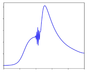
For large scale angles ( $\alpha > 6.8$), a wave packet as shown in figure 6 first appears at scale angle 6.8 close to the corner, and persists for larger scale angles. This wave packet appears similar to that of the two-dimensional case, described by Cassel et al. (Reference Cassel, Ruban and Walker1995) and also discussed by Exposito et al. (Reference Exposito, Gai and Neely2021). The studies of Smith & Bodonyi (Reference Smith and Bodonyi1985) and Tutty & Cowley (Reference Tutty and Cowley1986) provided the theoretical framework for inviscid instabilities arising as a consequence of the appearance of inflection points in velocity profiles. The numerical data of Cassel et al. (Reference Cassel, Ruban and Walker1995) and Fletcher, Ruban & Walker (Reference Fletcher, Ruban and Walker2004) supported this view. However, the study of Exposito et al. (Reference Exposito, Gai and Neely2021) showed that a similar wave packet could be triggered at stable flow conditions for values of the corner radius
 $r$ that induce a large pressure gradient. It must be noted here that Gittler & Kluwick (Reference Gittler and Kluwick1987) do not comment on the possibility of a wave packet in their study, which is probably due to their use of steady-state triple-deck equations.
(a) Pressure and (b) shear-stress distributions for scale angle  $\alpha = 7$ and scale external radius
 $R = 1$. Numerical configuration:
 $I = 401$,
 $J = 51$,
 $y_{max} = 16$.

Figure 7 shows scale angles at which a wave packet first appears, for different values of scale external radius. The same mesh ( $401 \times 51$) was employed in all cases. Since decreasing external radius causes significant flow expansion over the corner, a larger scale angle is needed to induce a pressure gradient and therefore trigger the appearance of a wave packet. These results seem to be in line with the observations of Li & Hao (Reference Li and Hao2023), who found that a decrease in cylinder radius delays the emergence of global instability. For an external radius of 10, the scale angle at which a wave packet is first observed is 3.8, very close to the two-dimensional value of 3.9 observed by Cassel et al. (Reference Cassel, Ruban and Walker1995) and 3.7 found by Fletcher et al. (Reference Fletcher, Ruban and Walker2004).
Scale angles at which a wave packet first appears for different values of scale radius (blue circles) and polynomial fit (blue solid line). Here,  $\alpha = 8.4, 6.8, 5.3, 4.6, 3.8$ and
 $R = 0.5, 1, 2.5, 5, 10$, respectively.

A trivial instability analysis equivalent to that of Tutty & Cowley (Reference Tutty and Cowley1986) for the axisymmetric case shows that the axisymmetric terms of the interaction law do not interfere in a meaningful manner with terms corresponding to the two-dimensional case. Therefore, we assumed that the mechanism through which the wave packet appears should be identical to that of the two-dimensional case, namely the appearance of an inflection point in the steamwise velocity profile close to the wall. Figure 8 shows velocity and  $\partial ^2 u / \partial y^2$ profiles at the corner for scale angles/scale radius pairs corresponding to those shown in figure 7. A coarse mesh
 $201\times 21$ needed to be employed to suppress the appearance of the wave packet, and the domain height was extended to
 $y_{max} = 50$. While profiles for scale external radius
 $R = 10$ are similar to those of Cassel et al. (Reference Cassel, Ruban and Walker1995), inflection points were not observed for any pair. Recent studies have suggested alternative mechanisms for the appearance of the wave packet. Exposito, Gai & Neely (Reference Exposito, Gai and Neely2022) found that the steady-state version of the algorithm of Cassel et al. (Reference Cassel, Ruban and Walker1995) generated spurious oscillations that do not correspond to a physical phenomenon. Another study by Exposito, Gai & Neely (Reference Exposito, Gai and Neely2023) suggested that the leading mechanism for the appearance of wave packets is a dispersive error created by the numerical algorithm owing to the presence of discontinuities in triple-deck solutions. Logue, Gajjar & Ruban (Reference Logue, Gajjar and Ruban2014) studied the stability of steady-state supersonic triple-deck flow over a compression corner and stated that an explanation for the appearance of the wave packet remained unavailable.
(a) Velocity and (b)  $\partial ^2 u / \partial y^2$ profiles for
 $\alpha = 8.4$ (blue),
 $6.8$ (cyan),
 $5.3$ (green),
 $4.6$ (yellow) and
 $3.8$ (red), and
 $R = 0.5, 1, 2.5, 5, 10$, respectively. Numerical configuration:
 $I = 201$,
 $J = 21$,
 $y_{max} = 50$.

More recently, Broadley, Hewitt & Gajjar (Reference Broadley, Hewitt and Gajjar2023) considered linear perturbations to the steady-state compression-ramp solution. They suggested that the eigenrelation provided by Tutty & Cowley (Reference Tutty and Cowley1986) could be temporarily met at a time snapshot during the unsteady evolution of the nonlinear solution, thereby producing a persistent wave packet that prevents a steady-state solution from being obtained with the unsteady equations. Our solutions seem to indicate that inflection points do not play an important role in the appearance of the wave packet; however, a more detailed study focusing on the unsteady flow evolution is necessary to ensure this. A steady-state and linear stability analysis akin to that of Broadley et al. (Reference Broadley, Hewitt and Gajjar2023) for the axisymmetric case could also improve our understanding of this problem.
5.3. External radius effects
Figure 9 shows the wall shear-stress (figure 9a) and pressure (figure 9b) distributions for scale external radius  $R = 10$ and scale angles
 $\alpha = 1, 2, 3$. For this configuration, a wave packet first appears for scale angles larger than 3.8. Curves are similar to those obtained for the two-dimensional case (Rizzetta et al. Reference Rizzetta, Burggraf and Jenson1978; Ruban Reference Ruban1978; Cassel et al. Reference Cassel, Ruban and Walker1995), albeit with minor axisymmetric effects. Regarding wall shear-stress values (figure 9a), axisymmetric effects are most noticeable for the largest scale angle downstream of the corner, where shear-stress values exceed those of the flat plate. For scale angles 1 and 2, the solution mirrors that of two-dimensional flow. Incipient separation is observed at a scale angle of 2.1, compared with the value of 1.9 for two-dimensional flow reported by Cassel et al. (Reference Cassel, Ruban and Walker1995). The over-expansion effect is noticeable in the pressure distribution downstream of the corner for all scale angles (figure 9b). The rate of decrease in pressure seems slightly larger downstream of the corner than at the right-hand side of the domain. This is probably due to the larger displacement function of the boundary layer close to the corner, which exacerbates axisymmetric effects.
(a) Wall shear-stress and (b) pressure distributions for scale external radius  $R=10$ and for scale angles
 $\alpha = 1, 2, 3$ from blue to red. Numerical configuration:
 $I = 401$,
 $J = 51$,
 $y_{max} = 16$.

Figure 10 shows the wall shear-stress (figure 10a) and pressure (figure 10b) distributions for scale radius  $R = 5$ and scale angles
 $\alpha = 1, 2, 3, 4$. The wave packet appears for scale angles larger than 4.6. Incipient separation is obtained for a scale angle of 2.5, which is larger than the value of 2.1 observed for scale external radius
 $R = 10$. The over-expansion effect is clearly more noticeable than for larger external scale radii, as can be seen in shear-stress values downstream of the corner. However, the flow structure within the separated region remains relatively similar to that of the two-dimensional case.
(a) Wall shear-stress and (b) pressure distributions for scale external radius  $R=5$ and scale angles
 $\alpha = 1, 2 , 3, 4$ from blue to red. Numerical configuration:
 $I = 401$,
 $J = 51$,
 $y_{max} = 16$.

Results for radius  $R = 1$ were shown in previous sections. Figure 11 shows results for radius
 $R = 0.5$ and scale angles
 $\alpha = 1, 2, 3, 4, 5, 6$. In this case, the wave packet appears for scale angles larger than 8.4. Incipient separation is first observed for scale angle 4. Shear-stress profiles shown in figure 11(a) suggest a flow structure similar to that of larger scale external radii. For equivalent scale angles, smaller separated regions are obtained compared with the two-dimensional case. The second shear-stress minimum similarly appears at a larger scale angle (6 compared with the value of 3.5 for two-dimensional flow). Pressure distributions, show in figure 11(b), are also similar to those of larger external radii but reduced in terms of magnitude due to the lower pressure gradient.
(a) Wall shear-stress and (b) pressure distributions for scale external radius  $R=0.5$ and scale angles
 $\alpha = 1, 2 , 3, 4, 5, 6$ from blue to red. Numerical configuration:
 $I = 401$,
 $J = 51$,
 $y_{max} = 16$.

Figure 12 shows results for radius  $R = 0.1$ and scale angles
 $\alpha = 1, 2, 3, 4, 5, 6$. No wave packet was observed for this value of scale external radius. Incipient separation was not obtained for the range of scale angles considered here, as can be seen in figure 12(a), showcasing shear-stress values. Due to the low value of
 $R$, the phenomenon of over-expansion is significant. The streamwise extent of the interaction is substantially smaller than that for
 $R=0.5$ and larger radii, suggesting that axisymmetric effects do not vary linearly with the inverse of
 $R$ but are more noticeable for
 $R<0.5$. For all scale angles, only one shear-stress minimum is obtained, which is then followed by a local maximum downstream of the corner. From figure 12(b), showing pressure values, it can be seen that this corresponds to the compression of the boundary layer downstream of the corner. Pressure values are much lower than that corresponding to larger radii; therefore indicating that larger scale angles are necessary to disturb the boundary layer as the scale external radius is reduced. The underlying assumption of the model, that the boundary layer height is much smaller than the external radius, should be invalid for sufficiently small values of
 $R$. Bodonyi, Smith & Kluwick (Reference Bodonyi, Smith and Kluwick1985) considered axisymmetric flow past a slender body where the boundary-layer thickness is of the order of the external radius and showed that a more complicated interaction (compared with the two-dimensional case) between the boundary layer and the external flow can potentially develop.
(a) Wall shear-stress and (b) pressure distributions for scale external radius  $R=0.1$ and scale angles
 $\alpha = 1, 2 , 3, 4, 5, 6$ from blue to red. Numerical configuration:
 $I = 401$,
 $J = 51$,
 $y_{max} = 16$.

6. Conclusions
The method of Ruban (Reference Ruban1978) and Cassel et al. (Reference Cassel, Ruban and Walker1995) was adapted to consider unsteady supersonic flow over an axisymmetric compression corner. The steady-state version of this problem had been considered earlier by Gittler & Kluwick (Reference Gittler and Kluwick1987). Scale external radii from 0.1 to 10 have been calculated. For scale external radii from 1 to 10, wall shear-stress and pressure distributions are similar to those corresponding to the two-dimensional case, except for minor axisymmetric effects in the form of shear-stress and pressure decrease in the limit  $x \rightarrow \infty$. For an external radius of 10, a wave packet first appears for scale angle values larger than 3.8, compared with the value of 3.9 for two-dimensional flow observed by Cassel et al. (Reference Cassel, Ruban and Walker1995). As the scale external radius decreases, the adverse pressure gradient over the corner is reduced due to the phenomenon of over-expansion as reported by Gittler & Kluwick (Reference Gittler and Kluwick1987). A larger scale angle is required to trigger the appearance of a wave packet. Inspection of
 $\partial ^2 u / \partial y^2$ profiles for scale external radius / scale angle pairs that first manifest a wave packet does not reveal an inflection point for any pair. The instability could be triggered during the unsteady evolution of the flow as suggested by Broadley et al. (Reference Broadley, Hewitt and Gajjar2023) for the two-dimensional case. To ascertain this, an analysis involving steady-state simulations and a stability analysis should be performed and compared with the unsteady solution.
For a scale external radius of 0.5, axisymmetric effects become important. Larger scale angles are necessary to produce a flow structure similar to that of the two-dimensional case. For example, the second shear-stress minimum manifests at a scale angle of 6, compared with the value of 3.5 for two-dimensional flow. For an external radius of 0.1, no second shear-stress minimum is observed. The streamwise extent of the interaction is lower than that corresponding to  $R=0.5$. Absolute shear-stress and pressure values are also reduced with decreasing external radius, corresponding to a weaker pressure perturbation due to larger axisymmetric effects.
Funding
The author gratefully acknowledges financial support from the National Natural Science Foundation of China (grant no. W2433020).
Declaration of interests
The author reports no conflict of interest.



