2.1. Problem description

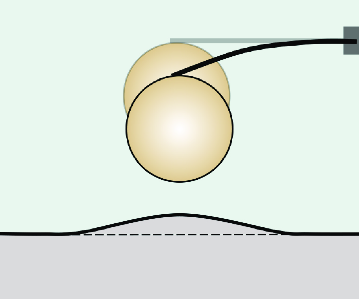
We first discuss the static problem. As shown in figure 1, one end of the cantilever is fixed to a piezo-actuated holder positioned at height $d$ above the undeformed surface of the test substrate. The opposite end of the cantilever is equipped with a spherical probe or tip of radius $R_s$ . The height of the holder can then be expressed as the sum of the cantilever deflection $\delta$ , the height of the probe $s$ , and a reference distance $d_{{ref}}$ :

(2.1) \begin{equation} d=\delta +s+d_{{ref}}. \end{equation}

Since $d_{{ref}}$ is a fixed, absolute distance that requires specific calibrations in experiments (Krieg et al. Reference Krieg, Fläschner, Alsteens, Gaub, Roos, Wuite, Gaub, Gerber, Dufrêne and Müller2019), we will disregard it and focus on the relative cantilever position (i.e. $d-d_{{ref}}$ ) in subsequent discussions.

Figure 1.

Jump-to-contact of an AFM probe with an elastic substrate influenced by surface tension. The probe, with radius $R_s$ , is mounted on a cantilever of spring constant $k$ . The cantilever is controlled by a holder positioned at height $d$ above the undeformed surface.

The cantilever deflection is caused by the attractive force $F$ between the probe and the substrate. Considering the cantilever stiffness $k$ , the deflection $\delta$ is given by

(2.2) \begin{equation} \delta = \frac {F}{k}. \end{equation}

The interaction force $F$ originates from intermolecular forces between the probe and the substrate across the intervening medium (typically air or liquid in AFM experiments):

(2.3) \begin{equation} F = 2\unicode{x03C0} \int _0^\infty p(r)r \,\mathrm{d} r. \end{equation}

In this work, we focus on non-retarded vdW forces and account for the substrate deformation $w(r)$ (see figure 1). The interaction force per unit area at location $r$ can then be described by

(2.4) \begin{equation} p(r) = \frac {4A R_s^3}{3\unicode{x03C0} \left [\left (s + R_s - w\right)^2 + r^2 - R_s^2\right]^3}, \end{equation}

according to Hamaker theory (Israelachvili Reference Israelachvili2011), where $A$ is the Hamaker constant. Finally, determining the substrate deformation requires solving the boundary value problem for an elastic half-space subjected to normal traction arising from vdW forces and surface tension, which is expressed as

(2.5) \begin{equation} \sigma _{zz}(r, z=0) = p(r) + \gamma\, \boldsymbol{\nabla} \cdot \boldsymbol{n}, \end{equation}

where $\boldsymbol{n}$ represents the normal vector to the deformed surface $z = w(r)$ of the elastic half-space, and $\gamma$ is the constant surface tension of the substrate surface. The full expression for the second term on the right-hand side of (2.5) is given by

(2.6) \begin{equation} \gamma \boldsymbol{\nabla} \cdot \boldsymbol{n} = \frac {\gamma }{r} \frac {{\mathrm{d}}}{\mathrm{d} r} \left ( \frac {r w^{\prime}}{\sqrt {1 + {w^{\prime}}^2}} \right), \end{equation}

where $w^{\prime}$ denotes $\mathrm{d} w / \mathrm{d} r$ .

The axisymmetric nature of the problem specified above allows it to be solved more conveniently by transforming it into the Hankel domain (Box et al. Reference Box, Jacquemot, Adda-Bedia and Vella2020; Essink et al. Reference Essink, Pandey, Karpitschka, Venner and Snoeijer2021). The $n$ th-order Hankel transform is defined as (Sneddon Reference Sneddon1995)

(2.7) \begin{equation} \tilde{f}(\xi) = \mathcal{H}_n[f(r)] = \int _0^\infty f(r) J_n(\xi r) r \,\mathrm{d} r, \end{equation}

with the inverse transform given by

(2.8) \begin{equation} f(r) = \mathcal{H}_n^{-1}[\tilde{f}(\xi)] = \int _0^\infty \tilde{f}(\xi)\, J_n(\xi r) \xi \,\mathrm{d} \xi. \end{equation}

In the Hankel domain, the linear elastic response of a semi-infinite elastic substrate is expressed as

(2.9) \begin{equation} \tilde{w}(\xi) = \frac {1 - \nu }{G \xi }\, \tilde{\sigma }_{zz}(\xi, z = 0), \end{equation}

where both $\tilde{w}(\xi)$ and $\tilde{\sigma }_{zz}$ correspond to the zeroth-order Hankel transform, and $\nu$ and $G$ are the Poisson’s ratio and shear modulus of the substrate, respectively (Hannah Reference Hannah1951; Sneddon Reference Sneddon1995). Note that this transformation method is essentially identical to the Green’s function method, but it is limited to axisymmetric geometries (Rallabandi Reference Rallabandi2024).

2.2. Non-dimensionalisation

Tabor & Winterton (Reference Tabor and Winterton1969) utilised rigid substrates and relatively large probes in their experiments to measure vdW forces. This set-up allows them to derive the analytical relations

(2.10) \begin{equation} F = \frac {A R_s}{6s^2} \quad \text{and} \quad d = s + \frac {A R_s}{6ks^2} \end{equation}

by substituting (2.4) into (2.3), assuming $w = 0$ and $s \ll R_s$ . In this rigid limit, the critical gap, force, and holder position at the onset of the jump can be directly obtained as

(2.11) \begin{equation} s_c = \frac {1}{3^{1/3}}\left (\frac {A R_s}{k}\right)^{1/3}, \quad F_c = \frac {1}{2 \times 3^{1/3}}(A k^2 R_s)^{1/3} \quad \text{and}\quad d_c = \frac {3^{1/3}}{2}\left (\frac {A R_s}{k}\right)^{1/3}. \end{equation}

While this work considers a soft, deformable substrate, we continue to use the characteristic lengths suggested by the rigid limit. This is because the measurements on soft substrates or thin flexible materials typically use very compliant cantilevers for improved force sensitivity (Wegmann et al. Reference Wegmann, Medalsy, Mandelkow and Müller2013; Krieg et al. Reference Krieg, Fläschner, Alsteens, Gaub, Roos, Wuite, Gaub, Gerber, Dufrêne and Müller2019; Dai et al. Reference Dai, Lu, Liechti and Huang2020). In this case, the induced deformation of the substrate remains small compared to the deflection of the cantilever (so it is the probe that jumps). We adopt the following vertical characteristic length, as suggested by (2.11),

(2.12) \begin{equation} s_*:= \left ( \frac {A R_s}{k} \right)^{1/3}, \end{equation}

which subsequently gives rise to the horizontal characteristic length by incorporating the probe geometry,

(2.13) \begin{equation} \ell _*:= (R_s s_*)^{1/2}. \end{equation}

Note that in typical experimental set-ups, $s_*$ can be tuned by varying the sphere radius and cantilever stiffness, with values spanning from a few nanometres to several microns, while $s_*$ is always much smaller than $\ell _*$ (Binnig et al. Reference Binnig, Quate and Gerber1986; Israelachvili & Tabor Reference Israelachvili and Tabor1972). Utilising (2.12) and (2.13), along with corresponding levels of vdW forces, we rescale the variables in real and Hankel spaces to introduce dimensionless variables:

(2.14) \begin{equation} \begin{aligned} & R=\frac {r}{\ell _*},\quad D=\frac {d}{s_*},\quad S=\frac {s}{s_*},\quad W=\frac {w}{s_*},\quad \mathcal{F}=\frac {Fs_*^2}{AR_s},\quad P=\frac {ps_*^3}{A},\\ & \Xi =\xi \ell _*,\quad \tilde{W}=\frac {\mathcal{H}_0[w]}{s_*\ell _*^2},\quad \tilde{P}=\frac {\mathcal{H}_0[p]s_*^2}{A\ell _*^2}. \end{aligned} \end{equation}

With (2.14), the problem specified in (2.1)–(2.9) can now be expressed as

(2.15) \begin{equation} D = \mathcal{F} + S, \end{equation}

where the attractive force between the probe and the deformed substrate is given by

(2.16) \begin{equation} \mathcal{F} = 2\unicode{x03C0} \int _0^\infty P(R) R \,\mathrm{d} R, \end{equation}

the dimensionless attractive vdW forces per unit area are given as

(2.17) \begin{equation} P(R) = \frac {4\alpha ^3}{3\unicode{x03C0} \left [\left (1 + \alpha S - \alpha W\right)^2 + \alpha R^2 - 1\right]^3}, \end{equation}

and the surface deformation satisfies the equilibrium equation in Hankel space,

(2.18) \begin{equation} \tilde{W}(\Xi)= \Gamma\, \mathcal{H}_1\left [\frac {R W_R}{\sqrt {1 + \alpha W_R^2}}\right] + (1 + \Gamma)\epsilon \frac {\tilde{P}(\Xi)}{\Xi }. \end{equation}

Here, we have integrated once to obtain the first term on the right-hand side of (2.18) (denoting nonlinear Laplace pressure caused by solid surface tension). In (2.18), we have defined the effective thickness of the gap beneath the probe as

(2.19) \begin{equation} \alpha:= \frac {s_*^2}{\ell _*^2}=\frac {s_*}{R_s}, \end{equation}

which is generally much less than unity. Therefore, $\alpha W_R^2$ in the Laplace pressure term in (2.18) will be dropped in numerics later in this study, such that $\mathcal{H}_1[RW_R]$ reduces to $-\Xi\, \tilde{W}(\Xi)$ . However, let us keep it in the analysis at this moment so that we will be able to illustrate that the small term associated with $\alpha$ is relatively more important in the vdW pressure than in the Laplace pressure.

In (2.18), we have also defined a parameter to characterise the effect of surface tension as

(2.20) \begin{equation} \Gamma:= \frac {(1-\nu)\gamma }{G\ell _*}, \end{equation}

which can be interpreted as an elasto-capillary number for elastic half-space systems (Style et al. Reference Style, Jagota, Hui and Dufresne2017; Bico et al. Reference Bico, Reyssat and Roman2018; Andreotti & Snoeijer Reference Andreotti and Snoeijer2020). Finally, we have introduced a parameter to characterise the effective compliance of the elastic substrate with solid surface tension in (2.18):

(2.21) \begin{equation} \epsilon:= \frac {A\ell _*^2}{G\ell _* s_*^4/(1-\nu)+\gamma s_*^4}=\frac {(1-\nu)AR_s^{1/2}}{(1+\Gamma)Gs_*^{7/2}}. \end{equation}

This effective compliance is defined by comparing the typical deformation of the substrate ( $w_*$ ) induced by the typical vdW force ( $p_*$ ) to the characteristic sphere–substrate gap $s_*$ , given in (2.12). The typical vdW force can be estimated by combining (2.12) and (2.4), resulting in $p_* \sim A / s_*^3$ in the regime where deformation is limited and the sphere is large. Estimating the typical substrate deformation requires some consideration, which we approach using an energy argument. Specifically, the external work done by vdW forces scales as $p_*\ell _*^2\, w_*$ . This work is stored as elastic energy, scaling as $G\varepsilon ^2 \, \ell _*^3$ , and as surface energy, scaling as $\gamma\, \Delta S$ , where the strain is $\varepsilon \sim w_*/\ell _*$ , and the increase in surface area is $\Delta S \sim w_*^2$ . By equating the stored energy to the external work, we find that $w_* \sim A\ell _*^2 / [(G\ell _* + \gamma)s_*^3]$ . This relationship yields (2.21) by comparing $w_*$ to $s_*$ (Poisson’s ratio is included for notational convenience).

Considering a typical soft gel with shear modulus $ G = 100$ kPa and Poisson’s ratio $ \nu = 0.5$ , along with a Hamaker constant $ A = 10^{-20}\,\mathrm{J}$ , solid surface tension $ \gamma = 10\,\mathrm{mN\, m^{-1}}$ , cantilever stiffness $ k = 0.1\,\mathrm{N\, m^{-1}}$ , and a spherical probe of radius $ R_s = 10\,{\unicode{x03BC} \mathrm{m}}$ , the characteristic scales are approximately $ s_* \approx 10\,\mathrm{nm}$ and $ \ell _* \approx 316\,\mathrm{nm}$ , yielding $ \alpha \approx 10^{-3}$ , $ \Gamma \approx 1.58$ and $ \epsilon \approx 0.61$ . Notably, ultrasoft cantilevers with stiffness $ k \sim 0.01\,\mathrm{N\, m^{-1}}$ are often employed to achieve high-resolution AFM imaging with enhanced force sensitivity (Wegmann et al. Reference Wegmann, Medalsy, Mandelkow and Müller2013), where $ \epsilon \sim 0.05$ . It is also worth noting that we have assumed linear elasticity for the substrate in the model. This assumption should be valid in typical colloidal AFM experiments since the strain scales as ${w_*}/{\ell _*}=\alpha \,\epsilon$ , which is small even when $\epsilon =\mathcal{O}(1)$ .

2.3. Numerical solution

The problem defined by (2.15)–(2.18) depends solely on three dimensionless physical parameters: $\alpha$ , $\Gamma$ and $\epsilon$ . Since $\alpha \ll 1$ in typical experiments, the focus lies in understanding the jump-to-contact behaviour of substrates with varying compliance $\epsilon$ under different surface effects $\Gamma$ . In all calculations, we let $\alpha = 10^{-2}$ (unless otherwise specified), as further reducing its value does not yield any noticeable changes in the numerical results. We solve this problem numerically using a uniform grid (refined near the origin) and the standard iterative method (Press et al. Reference Press, Teukolsky, Vetterling and Flannery2007). A grid with 5000 points over the real and Hankel domains $[10^{-3}, 10^{3}]$ can ensure convergence for the parameters considered in this work. It is worth mentioning that while experimental operations typically involve prescribing $D$ and measuring $S$ , it is computationally more convenient to prescribe the gap $S$ and solve for $D$ . This approach avoids complications arising from the existence of two solutions for a given $D$ (one stable and the other unstable, to be discussed with figure 2).

3.1. Perturbation method

Although the problem is intrinsically nonlinear due to the vdW force, analytical progress can be made when $\epsilon$ is small. Note again that force measurements in AFM experiments can benefit from soft cantilevers (i.e. small values of $\epsilon$ ). Specifically, based on the equilibrium equation (2.18), we conduct a perturbation analysis for the surface deformation and the vdW pressure, adopting the structure

(3.1) \begin{equation} W(R) = W_0(R) + \epsilon W_1(R) + O(\epsilon ^2), \quad P(R) = P_0(R) + \epsilon P_1(R) + O(\epsilon ^2). \end{equation}

Substituting (3.1) into (2.18) yields

(3.2) \begin{align} &\epsilon ^0 \left ( \tilde{W}_0 - \Gamma\, \mathcal{H}_1 \left [ \frac {R W_0^{\prime}}{\sqrt {1 + \alpha {W_0^{\prime}}^2}} \right] \right) \notag\\ &\qquad + \epsilon ^1 \left ( \tilde{W}_1 - \Gamma \mathcal{H}_1 \left [ \frac {R W_1^{\prime}}{\sqrt {1 + \alpha {W_0^{\prime}}^2}} \right] - (1 + \Gamma) \frac {\tilde{P}_0(\Xi)}{\Xi } \right) + \cdots = 0, \end{align}

which leads to the results

(3.3) \begin{equation} \tilde{W}_0 = 0, \quad \tilde{W}_1 = \frac {(1 + \Gamma) \tilde{P}_0}{\Xi (1 + \Gamma \Xi)}. \end{equation}

Clearly, the nonlinear term in the Laplace pressure does not influence the solution up to $O(\epsilon ^2)$ . Using this, the expression obtained by substituting (3.1) into (2.4) can be simplified as

(3.4) \begin{equation} \epsilon ^0 \left ( P_0 - \frac {4}{3 \unicode{x03C0} (R^2 + 2 S + \alpha S^2)^3} \right) + \epsilon ^1 \left ( P_1 - \frac {8 (1 + \alpha S) W_1}{\unicode{x03C0} (R^2 + 2 S + \alpha S^2)^4} \right) + \cdots = 0. \end{equation}

Combining (3.3) and (3.4), we obtain the zeroth-order solution

(3.5) \begin{equation} W_0 = 0, \quad P_0 = \frac {4}{3 \unicode{x03C0} (R^2 + 2 S + \alpha S^2)^3}, \end{equation}

and the first-order solution

(3.6) \begin{equation} W_1 = \mathcal{H}_0^{-1} \left [ \frac {\text{K}_2\left (\sqrt {S (2 + \alpha S)}\, \Xi \right)}{6 \unicode{x03C0} S (2 + \alpha S)} \frac {(1 + \Gamma) \Xi }{1 + \Gamma \Xi } \right], \quad P_1 = \frac {8 (1 + \alpha S)}{\unicode{x03C0} (R^2 + 2 S + \alpha S^2)^4} W_1, \end{equation}

where $ \text{K}_n$ denotes the modified Bessel function of the $ n$ th kind. While the first-order solution cannot be expressed analytically, we derive approximate analytical solutions within small and large surface tension limits.

Figure 2.

Substrate deformation and the fold bifurcation. (a) Surface deformation of the elastic substrate for various gap values, as indicated by the colour bar. Markers represent numerical results, while solid curves correspond to the analytical solution given in (3.7). Only solid markers indicate stable and physically meaningful solutions, as the gaps for empty markers fall below the critical jump gap $S_c$ . (b) Gap as a function of the cantilever position for rigid (black curve, see (2.10)) and deformable (red curve, see (3.8)) substrates. Empty markers represent numerical results, while the two solid markers indicate the critical gap and the corresponding cantilever position where jump-to-contact occurs. All calculations are performed with $ \alpha = 0.01$ , $ \epsilon = 0.1$ and $ \gamma = 0.1$ .

3.2. Small surface tension

We first consider the case of small $\Gamma$ , allowing $(1+\Gamma)\Xi /(1+\Gamma \Xi)$ in the right-hand side of the first term in (3.6) to be approximated as $\Xi + \Gamma \Xi - \Gamma \Xi ^2$ . With this approximation, the inverse Hankel transform in (3.6) can be readily carried out, yielding

(3.7) \begin{align} W_1 &= \frac {1 + \Gamma }{6 \unicode{x03C0} S^{3/2} (2 + \alpha S)^{3/2} W_s^2} \notag\\ &\quad \times \left [ 2 (2W_s - R^2)\,\mathcal{E}\left (\frac {-R^2}{2 S + \alpha S^2}\right) - W_s\,\mathcal{K}\left (\frac {-R^2}{2 S + \alpha S^2}\right) \right] - \frac {4\Gamma }{3 \unicode{x03C0} W_s^3}, \end{align}

where $W_s(R) = 2S + \alpha S^2 + R^2$ , and $\mathcal{K}$ and $\mathcal{E}$ represent the elliptic integrals of the first and second kind, respectively. This solution, along with the first equation in (3.1), shows good agreement with the numerically calculated substrate deformation presented in figure 2(a), which is obtained using $ \alpha = 0.01$ , $ \epsilon = 0.1$ , $ \gamma = 0.1$ and various values of $S$ .

However, not all values of $S$ are physically meaningful, due to the jump-to-contact instability. This can be seen further by substituting (3.7) into the second equation of (3.6), and then combining (3.1) with (2.16), giving

(3.8) \begin{align} \mathcal{F}={}&\frac {2}{3 S^2 (2 + \alpha S)^2} \nonumber \\ &{}+ \left [ \frac {315 \unicode{x03C0} }{2048 \left (2S + \alpha S^2\right)^{11/2}} - \frac {32\,768 - 2835 \unicode{x03C0} ^2 \sqrt {S (2 + \alpha S)}}{18\,432\, \unicode{x03C0} S^6 (2 + \alpha S)^6} \Gamma \right](1 + \alpha S)\epsilon. \end{align}

Using this solution and the relation $D = S + \mathcal{F}$ from (2.15), we plot the gap between the probe and the undeformed substrate as a function of the AFM cantilever holder position in figure 2(b). As before, there is good agreement between the analytical solution (solid and dashed curves) and the numerical results (empty markers). In addition, a saddle-node (fold) bifurcation structure is observed (similar to pull-in instability in micro-electromechanical systems; Gomez, Moulton & Vella Reference Gomez, Moulton and Vella2017b ; Li, Yu & Dai Reference Li, Yu and Dai2024): for a typical given holder position, two gap solutions typically exist, with only the solution corresponding to the larger gap (i.e. the solid curves in figure 2 b) being stable. As the cantilever approaches the substrate, the stable solution eventually disappears at the point $(S_c, D_c, \mathcal{F}_c)$ , where it merges with the unstable solution (dashed curve) and the probe jumps into contact with the substrate.

Figure 3.

Premature jump-to-contact on compliant substrates. (a) The gap under the probe and (b) the net attractive vdW force, as functions of the cantilever position for substrates with different compliances $\epsilon$ (encoded in the colour bar). Coloured empty markers represent numerical calculations, while the coloured curves are based on (2.15) and (3.8). The leftmost curve in black represents the rigid limit, as given by (2.10). Here, $\alpha =0.01$ and $\Gamma =0.1$ .

Compared to a rigid substrate, a compliant substrate undergoes surface deformation during the cantilever’s approach. Such deformation enhances the effective strength of vdW forces, causing jump-to-contact to occur prematurely, as shown in figure 2(b). This behaviour is further illustrated in figure 3, where the gap and net vdW attraction are plotted as functions of the cantilever position for substrates with various effective compliances $\epsilon$ . For the numerical calculations, we used $\Gamma = 0.1$ and $\alpha = 0.01$ , which show good agreement with the analytical solution given by (3.8) in combination with (2.15) for small $\epsilon$ . As the substrate compliance vanishes, the results converge to the rigid limit (black curves in figure 3) described by (2.10). For substrates with finite compliance, deformation induced by vdW forces leads to a premature jump-to-contact, corresponding to larger critical gaps and cantilever positions as well as smaller critical attractive forces. This clearly indicates that substrate deformation must be carefully accounted for when measuring the vdW interaction or surface adhesion of relatively soft materials using AFM (Krieg et al. Reference Krieg, Fläschner, Alsteens, Gaub, Roos, Wuite, Gaub, Gerber, Dufrêne and Müller2019). For instance, fitting experimental force curves with a rigid substrate model could lead to an overestimation of the interaction between tissues or living cells and probes coated with nanocarriers (Friedrichs, Helenius & Muller Reference Friedrichs, Helenius and Muller2010; Yu et al. Reference Yu, Zeng, Wang, Cui, Gao, Yin, Liu, Wei, Wei and Dai2025).

In figure 4, we present the critical force $\mathcal{F}_c$ and the critical cantilever position $D_c$ at the onset of the jump for substrates, with varying compliances and surface tensions. For small values of $\Gamma$ and $\alpha$ , the critical gap can also be estimated analytically. Specifically, from (2.15) and (3.8), we obtain

(3.9) \begin{equation} S_c \approx \frac {1}{3^{1/3}} {- \frac {\alpha }{6 \times 3^{2/3}}}+ \frac {3465 \times 3^{5/6} \unicode{x03C0} }{131\,072\, \sqrt {2}} \left (1 - 0.085\,\Gamma \right) \epsilon, \end{equation}

which further leads to

(3.10a) \begin{align} \mathcal{F}_c \approx \frac {1}{2 \times 3^{1/3}} {- \frac {3^{1/3}}{9}\alpha } - \frac {1575 \times 3^{5/6} \unicode{x03C0} }{131\,072\, \sqrt {2}} \left (1 - 0.19\,\Gamma \right) \epsilon, \end{align}

(3.10b) \begin{align} D_c \approx \frac {3^{2/3}}{2} {- \frac {3^{1/3}}{6}\alpha } + \frac {945 \times 3^{5/6} \unicode{x03C0} }{65\,536\, \sqrt {2}} \left (1 + 0.0055\,\Gamma \right) \epsilon. \end{align}

The decimal coefficients in (3.9) and (3.10) arise from combining analytic factors into a compact decimal form to simplify the presentation. These analytical results are consistent with the surface-tension-free solutions reported recently in Yu & Dai (Reference Yu and Dai2024) as $\Gamma \to 0$ . They also show good agreement with numerical calculations for various $\epsilon$ and $\Gamma$ , when these values remain sufficiently small (figure 4). It is noteworthy that the compliance defined in (2.21) incorporates contributions from both solid surface tension and elasticity. Under this unified definition, the prefactors of $\Gamma$ in $S_c$ and $D_c$ are found to be relatively small. In contrast, the additional influence of $\Gamma$ on $\mathcal{F}_c$ is more significant, causing the analytical approximation of $\mathcal{F}_c$ in (3.10a ) to become invalid for $\Gamma \gtrsim 1$ (see figure 4 a). We now shift our focus to the case of large surface tension.

Figure 4.

The jump-to-contact point for substrates with small surface tensions ( $\Gamma \ll 1$ ). (a) Critical attractive vdW force $\mathcal{F}_c$ and (b) critical cantilever position $D_c$ , as functions of the effective compliance of the substrate $\epsilon$ , as defined in (2.21). Markers represent numerical calculations, while curves correspond to the analytical solutions given in (3.10a ) and (3.10b ) for various surface tension values $\Gamma$ . The specific values of $\Gamma$ are indicated by the colour bar. Note that the solid curves remain valid only for small $\Gamma$ ; at $\Gamma =10$ , they exhibit significant deviations from the marker data. Here, we used $\alpha =0.01$ in numerics.

3.3. Large surface tension

Within the limit of large surface tension, the term ${(1 + \Gamma) \Xi }/{(1 + \Gamma \Xi)}$ in the right-hand side of the first term in (3.6) approximates to $1$ . However, the inverse Hankel transform $\text{K}_2 (\sqrt {S (2 + \alpha S)}\, \Xi)$ is unbounded. To understand this issue, we go back to the first-order equation in (3.2), i.e.

(3.11) \begin{equation} \Xi \tilde{W}_1(\Xi)+ \Gamma \Xi ^2\, \tilde{W}_1(\Xi) ={(1 + \Gamma)\tilde{P}_0}(\Xi), \end{equation}

and examine it with $\Gamma \gg 1$ directly in real space:

(3.12) \begin{equation} \frac {1}{R}\frac {\mathrm{d} }{\mathrm{d} R}\left (R \frac {\mathrm{d} W_1^{(i)}}{\mathrm{d} R}\right) + \frac {4}{3 \unicode{x03C0} \left (R^2 + 2 S + \alpha S^2\right)^{3}} = 0. \end{equation}

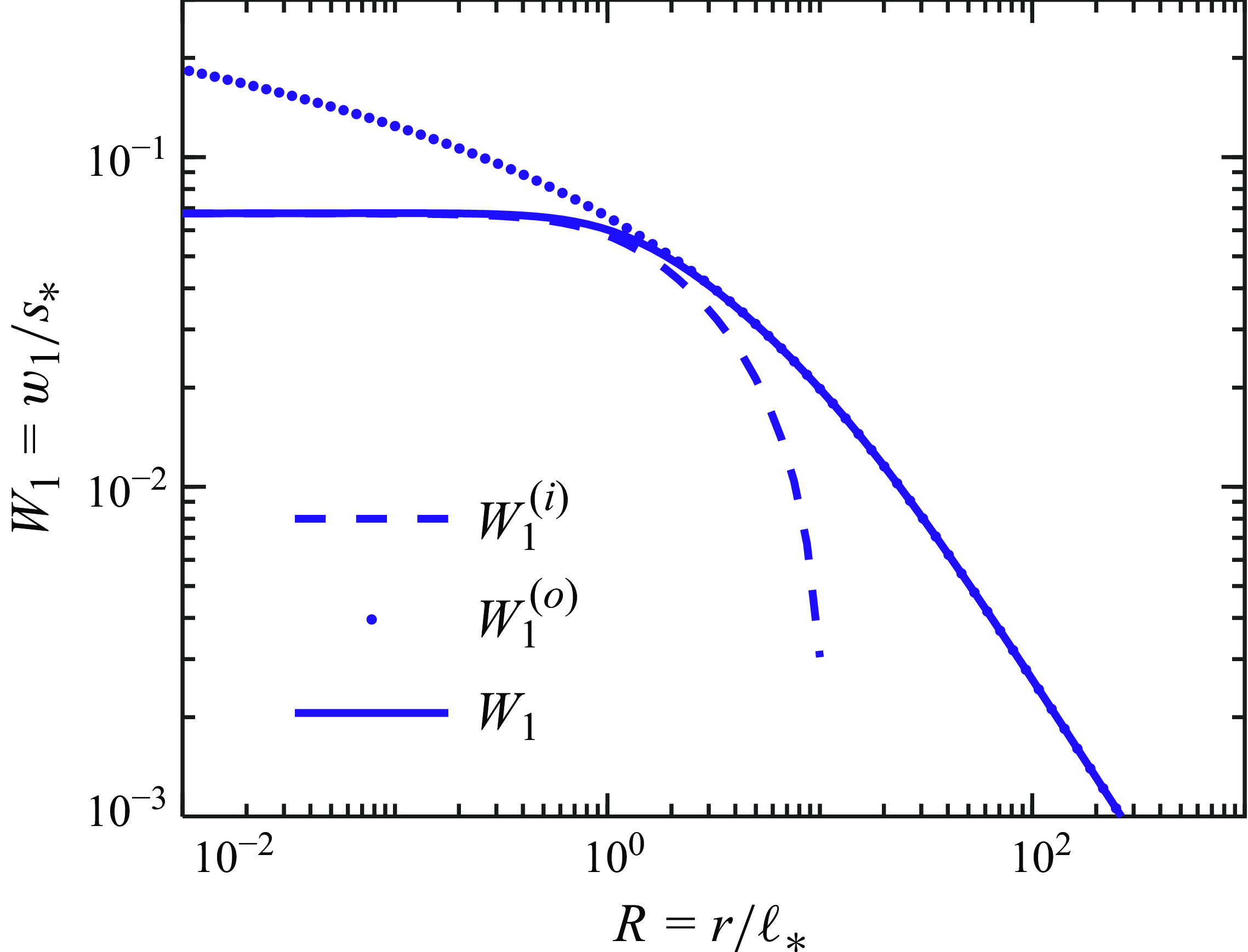
Here, the superscript $(i)$ denotes the ‘inner’ solution, as we will see that $W_1^{(i)}(R) \propto -\ln R$ when $R \to \infty$ and hence an ‘outer’ solution is required to ensure consistency over the entire domain. Physically, this inner solution neglects elasticity and thus represents a balance between Laplace pressure and the zeroth-order vdW pressure (Dai & Vella Reference Dai and Vella2022). The solution to (3.12) is given by

(3.13) \begin{equation} W_1^{(i)}(R) = C_1 + \frac {1}{6 \unicode{x03C0} S(2 + \alpha S)\,W_s(R)} + \frac {\left [2 + 6 \unicode{x03C0} C_2 S^2 (2 + \alpha S)^2 \right] \ln R - \ln W_s(R)}{6 \unicode{x03C0} S^2 (2 + \alpha S)^2}, \end{equation}

where $W_s(R) = 2S + \alpha S^2 + R^2$ , and $C_1$ and $C_2$ are integration constants. Imposing the symmetry condition at the origin, i.e. $\lim _{R \to 0} W^{\prime}(R) = 0$ , gives $C_2 =$ $-{1}/[{3\unicode{x03C0} S^2(2+\alpha S)^2}]$ .

To determine $C_1$ , we note that elasticity can eventually become important at large distances from the origin, playing a role in flattening the surface deformation similar to that of gravity. Indeed, the similar behaviour has been observed in the jump of an AFM probe to a liquid surface, where surface forces compete with gravity (Liu et al. Reference Liu, Bai, Xia and Ke2005; Quinn et al. Reference Quinn, Feng and Stone2013). We then rescale the radial variable in (3.11) as $\hat {R}=R/\Gamma$ and $\hat {\Xi }=\Gamma \Xi$ , resulting in

(3.14) \begin{equation} \hat {\Xi }\tilde{W}_1^{(o)}(\hat {\Xi }) + \hat {\Xi }^2\, \tilde{W}_1^{(o)}(\hat {\Xi }) = \frac {\hat {\Xi }^2\, \text{K}_2\left (\sqrt {S (2 + \alpha S)}\, \hat {\Xi }/\Gamma \right)}{6 \unicode{x03C0} S (2 + \alpha S)}, \end{equation}

which indicates that in the far-field limit ( $\hat {R} \sim 1$ or $\hat {\Xi } \sim 1$ ), elastic and surface forces are equally important. We solve (3.14) under the condition $\Gamma \gg 1$ , yielding the solution

(3.15) \begin{equation} {W}_1^{(o)}(\hat {R}) = \frac {\mathcal{G}\left ( {4}/{\hat {R}^2} \right)}{3 \unicode{x03C0} ^2 S^2 \left ( 2 + \alpha S \right)^2 \hat {R}}, \end{equation}

where $\mathcal{G}(x) = \text{MeijerG} ( \left \{ [0, {1}/{2}, {1}/{2}], [] \right \}, \left \{ [0], [] \right \}, \left \{ x \right \})$ , and $\text{MeijerG}$ represents the Meijer G function (§§ 5.3–5.6 in Bateman & Erdélyi Reference Bateman and Erdélyi1953). To match the inner solution with the outer solution, we impose

(3.16) \begin{equation} \lim _{R \to \infty } W_1^{(i)} = \lim _{\hat {R} \to 0} W_1^{(o)}, \end{equation}

which gives $C_1 = C_2 (\gamma _E - \log {2\Gamma })$ , where $\gamma _E$ is the Euler’s constant, with approximate value $0.577$ .

Finally, we obtain the valid first-order solution for the surface deformation of a surface-tension-dominated elastic substrate by combining the inner and outer solutions and subtracting their overlap (i.e. either side of (3.16)):

(3.17) \begin{align} W_1(R) ={} &\frac {1}{6\unicode{x03C0} S(2+\alpha S)(2S + \alpha S^2 + R^2)} \nonumber \\[5pt] &{} + \frac {2\Gamma \, \mathcal{G}\left ( {4\Gamma ^2}/{R^2} \right) - {\unicode{x03C0}R} \log {\left [ {(2S + \alpha S^2 + R^2)}/{R^2} \right]}}{6 \unicode{x03C0} ^2 S^2 (2 + \alpha S)^2 R}, \end{align}

which is plotted in figure 5. We compare this analytical solution to numerical results computed with $\epsilon = 0.1$ for various probe–substrate gaps, as shown in figure 6(a). Consistent with (3.14), the length scale over which the deformation decays is proportional to $\Gamma$ (see the comparison between $\Gamma = 10^2$ and $\Gamma = 10^4$ in figure 6 a).

Figure 5.

The first-order solution for the surface deformation of an elastic substrate influenced by large surface tension. The inner solution, outer solution and full solution are provided in (3.13), (3.15) and (3.17), respectively.

Figure 6.

The effect of surface tension on the substrate deformation. (a) Surface deformation of the elastic substrate for various gap values. Markers denote numerical results, while solid curves represent the analytical solution from (3.17). (b) Gap as a function of the cantilever position for rigid (black curve, given by (2.10)) and deformable (red curve, given by (3.18)) substrates. Calculations are performed with $\alpha = 0.01$ , $\epsilon = 0.05$ and $\Gamma = 10^2$ (or $\Gamma = 10^4$ , with corresponding markers and curves displayed with partial transparency).

Interestingly, increasing $\Gamma$ appears to enhance the extent of substrate deformation, thereby slightly advancing the jump-to-contact point, as illustrated in figure 6(a,b). However, this observation is nuanced: while $\epsilon$ is held constant, $\Gamma$ is embedded in the definition of $\epsilon$ through (2.21). Thus the results indeed suggest that surface tension mitigates premature jumps. Specifically, with $\epsilon$ fixed at $0.1$ , increasing $\Gamma$ from $10^2$ to $10^4$ needs to amplify the Hamaker constant (i.e. the strength of vdW interaction) by a factor of $100$ , yet the jump-to-contact point shifts only modestly (figure 6). This subtle behaviour arises because the prefactors for the jump-to-contact point depend on $\Gamma$ logarithmically, as will be discussed shortly.

Figure 7.

(a) The gap of the probe above the undeformed substrate and (b) the net attractive vdW force between the probe and the deformed substrate as functions of the cantilever position for substrates with different compliances $\epsilon$ (encoded in the colour bar). Coloured empty markers represent numerical calculations, while the coloured curves are based on (2.15) and (3.18). The leftmost curve in black represents the rigid limit, provided by (2.10). Here, $\alpha =0.01$ and $\Gamma =10$ .

To gain analytical insight into the jump-to-contact point, we use (3.6) to calculate $P_1$ , and subsequently employ (2.16) to calculate the total vdW force, given by

(3.18) \begin{align} \mathcal{F} ={}& \frac {2}{3 S^2 (2 + \alpha S)^2} \nonumber \\ &{}+ \left [12\log {\frac {4\Gamma ^2}{2S+\alpha S^2}} + 5 - 24\gamma _E + \frac {9\unicode{x03C0} \sqrt {2S+\alpha S^2}}{2\Gamma }\right]\frac {(1+\alpha S)\epsilon }{27 \unicode{x03C0} S^5 (2 + \alpha S)^5}. \end{align}

This relation, combined with (2.15), provides accurate predictions of the gap–cantilever position and force–cantilever position relationships for $\epsilon \ll 1$ and $\Gamma \gg 1$ , as demonstrated in figure 7. Furthermore, for $\alpha \ll 1$ , we are able to derive simple expressions for the critical gap, force and cantilever position at the onset of the jump as

(3.19a) \begin{align} S_c &\approx \frac {1}{3^{1/3}} \left (1 {- \frac {\alpha }{6 \times 3^{1/3}}} + \frac {120\log \Gamma + 20\log {24} + 37 - 120\gamma _E}{288\unicode{x03C0} }\epsilon \right),\\[-5pt]\nonumber \end{align}

(3.19b) \begin{align} \mathcal{F}_c &\approx \frac {1}{24^{1/3}} \left (1 {- \frac {2\times 3^{2/3}}{9}\alpha } - \frac {\log \Gamma + 0.41}{3\unicode{x03C0} }\epsilon \right),\\[-5pt]\nonumber \end{align}

(3.19c) \begin{align} D_c &\approx \frac {3^{2/3}}{2} \left (1 {- \frac {\alpha }{3}} + \frac {\log \Gamma + 0.16}{6\unicode{x03C0} }\epsilon \right), \end{align}

respectively. Again, the decimal coefficients here are exact values. These analytical solutions show good agreement with numerical results for substrates with low effective compliance, as illustrated in figure 8(a,b).

Figure 8.

The jump-to-contact point for substrates with large surface tensions ( $\Gamma \gg 1$ ). (a) Critical attractive vdW force $\mathcal{F}_c$ and (b) critical cantilever position $D_c$ as functions of the effective compliance of the substrate $\epsilon$ , for various surface tensions. Markers represent numerical calculations, while curves correspond to the analytical solutions given in (3.19a – c ). The values of corresponding surface tension are encoded in the colour bar. Note that the solid curves are valid only for large $\Gamma$ . Here, $\alpha =0.01$ is used in numerics.