1 Introduction
Particle-laden turbulent flows are ubiquitous phenomena in both nature and industry. Rain drops and aerosol particles in the atmosphere, sediment transport in rivers, and pneumatic transport of solid particles are just a few examples of particle-laden turbulent flows (Crowe et al. Reference Crowe, Schwarzkopf, Sommerfeld and Tsuji2011). Despite their importance and abundance, a generally applicable theory or model that can predict the behaviour of particle-laden turbulent flows is still not available (Poelma, Westerweel & Ooms Reference Poelma, Westerweel and Ooms2007). One of the challenges in improving understanding is the complex two-way interaction between turbulence and particles, by processes such as condensation–evaporation, heat exchange and drag force. Particles are dispersed and affected by the surrounding fluid, but, at the same time, they also affect the surrounding fluid through these processes.
The particle–turbulence interaction by the drag force is one of the simplest, but important, examples of two-way interaction. Since the pioneering works by Squires & Eaton (Reference Squires and Eaton1993), Elghobashi & Truesdell (Reference Elghobashi and Truesdell1993) and Sundaram & Collins (Reference Sundaram and Collins1999), this system has been investigated in various studies using statistical analysis, direct numerical simulation (DNS) and laboratory experimentation (Balachandar & Eaton Reference Balachandar and Eaton2010). Nevertheless, a clear understanding of the interaction has not yet been obtained. Many parameters have been proposed for characterizing the interaction, such as mass-loading parameter, Stokes number, Reynolds number and particle moment number (Tanaka & Eaton Reference Tanaka and Eaton2008). However, how quantitatively the fluid turbulence is modulated by particles depending on these parameters remains unclear.
In the present study, we introduce a new time scale for turbulence modulation by particles. The time scale is inversely proportional to the number density and the radius of particles, and can be regarded as a counterpart of the phase relaxation time in cloud physics. By a scaling analysis and DNS, we demonstrate that the new time scale is a crucial parameter for the quantitative understanding of turbulence modulation by particles.
2 Governing equations
Particles are regarded as spherical point masses. The evolution equations for the position and the velocity of the
 $j$
th particle are
 $$\begin{eqnarray}\displaystyle & \displaystyle \frac{\text{d}\boldsymbol{X}_{j}}{\text{d}t}=\boldsymbol{V}_{j}, & \displaystyle\end{eqnarray}$$
 $$\begin{eqnarray}\displaystyle & \displaystyle \frac{\text{d}\boldsymbol{V}_{j}}{\text{d}t}=\frac{\boldsymbol{u}(\boldsymbol{X}_{j})-\boldsymbol{V}_{j}}{\unicode[STIX]{x1D70F}_{p}}, & \displaystyle\end{eqnarray}$$
respectively, where
 $\boldsymbol{u}(\boldsymbol{X}_{j})$
is the fluid velocity at the particle position,
 $\unicode[STIX]{x1D70F}_{p}$
is the inertial response time, defined as
 $$\begin{eqnarray}\displaystyle \unicode[STIX]{x1D70F}_{p}=\frac{2\unicode[STIX]{x1D70C}_{p}r^{2}}{9\unicode[STIX]{x1D70C}_{f}\unicode[STIX]{x1D708}}, & & \displaystyle\end{eqnarray}$$
 $r$
is the particle radius,
 $\unicode[STIX]{x1D708}$
is the kinematic viscosity, and
 $\unicode[STIX]{x1D70C}_{p}$
and
 $\unicode[STIX]{x1D70C}_{f}$
are the particle and fluid densities, respectively. For the benefit of simplicity, particles are assumed to be mono-dispersed. The velocity field of a fluid is governed by the incompressible Navier–Stokes equations:
 $$\begin{eqnarray}\displaystyle & \displaystyle \frac{\unicode[STIX]{x2202}\boldsymbol{u}}{\unicode[STIX]{x2202}t}+\boldsymbol{u}\boldsymbol{\cdot }\unicode[STIX]{x1D735}\boldsymbol{u}=-\frac{\unicode[STIX]{x1D735}p}{\unicode[STIX]{x1D70C}_{f}}+\unicode[STIX]{x1D708}\unicode[STIX]{x1D6FB}^{2}\boldsymbol{u}+\boldsymbol{F}_{p}+\boldsymbol{f}_{ext}, & \displaystyle\end{eqnarray}$$
 $$\begin{eqnarray}\displaystyle & \displaystyle \unicode[STIX]{x1D735}\boldsymbol{\cdot }\boldsymbol{u}=0, & \displaystyle\end{eqnarray}$$
where
 $p$
is the pressure and
 $\boldsymbol{f}_{ext}$
represents the external force. Here
 $\boldsymbol{F}_{p}$
is the drag force exerted by particles on the surrounding fluid (Sundaram & Collins Reference Sundaram and Collins1999) and is defined by
 $$\begin{eqnarray}\displaystyle \boldsymbol{F}_{p}=-\frac{1}{\unicode[STIX]{x1D70C}_{f}}\mathop{\sum }_{j=1}^{N_{p}}m_{p}\left[\frac{\boldsymbol{u}(\boldsymbol{X}_{j})-\boldsymbol{V}_{j}}{\unicode[STIX]{x1D70F}_{p}}\right]\unicode[STIX]{x1D6FF}(\boldsymbol{x}-\boldsymbol{X}_{j}), & & \displaystyle\end{eqnarray}$$
where
 $N_{p}$
is the number of particles,
 $m_{p}=4\unicode[STIX]{x1D70C}_{p}\unicode[STIX]{x03C0}r^{3}/3$
is the particle mass, and
 $\unicode[STIX]{x1D6FF}()$
is the Dirac delta function. Here, the suspension is assumed to be dilute so that the effect of particle/particle collisions is negligible (Elghobashi Reference Elghobashi1994).
3 Theory
3.1 Flow relaxation time
We consider the time scale for the drag force exerted by particles on the surrounding fluid. In order to extract the importance of the time scale in its simplest form, we assume that particles are uniformly randomly distributed in the domain with their positions fixed in space, just like unmoving obstacles (Vreman Reference Vreman2016). The drag force in (2.6) is then reduced to
 $$\begin{eqnarray}\displaystyle \boldsymbol{F}_{p}=-\mathop{\sum }_{j=1}^{N_{p}}(6\unicode[STIX]{x03C0}\unicode[STIX]{x1D708}r)\boldsymbol{u}(\boldsymbol{X}_{j})\unicode[STIX]{x1D6FF}(\boldsymbol{x}-\boldsymbol{X}_{j}). & & \displaystyle\end{eqnarray}$$
We divide the domain into small subdomains and assume that each subdomain includes only a single particle (Tagawa et al.
Reference Tagawa, Mercado, Prakash, Calzavarini, Sun and Lohse2012). Since particles are assumed to be uniformly randomly distributed in the domain, the volume of the subdomain can be estimated approximately as
 $1/n_{p}$
, where
 $n_{p}$
is the number density of particles (the number of particles in a unit volume of the fluid). If we consider a certain subdomain and assume a uniform flow velocity in it, the drag force exerted by the particle onto the surrounding fluid is estimated by
 $$\begin{eqnarray}\frac{-(6\unicode[STIX]{x03C0}\unicode[STIX]{x1D707}r)\boldsymbol{u}}{\unicode[STIX]{x1D70C}_{f}(1/n_{p})}=-(6\unicode[STIX]{x03C0}\unicode[STIX]{x1D708}r)n_{p}\boldsymbol{u}\end{eqnarray}$$
per unit mass of the fluid, where
 $\unicode[STIX]{x1D707}=\unicode[STIX]{x1D708}\unicode[STIX]{x1D70C}_{f}$
is the dynamic viscosity. Therefore,
 $\boldsymbol{F}_{p}$
can be approximated by
 $$\begin{eqnarray}\displaystyle \boldsymbol{F}_{p}\sim -(6\unicode[STIX]{x03C0}\unicode[STIX]{x1D708}n_{p}r)\boldsymbol{u}=-\unicode[STIX]{x1D70F}_{f}^{-1}\boldsymbol{u}, & & \displaystyle\end{eqnarray}$$
where
 $\unicode[STIX]{x1D70F}_{f}$
is the relaxation time for the fluid velocity field and is defined as
 $$\begin{eqnarray}\displaystyle \unicode[STIX]{x1D70F}_{f}=(6\unicode[STIX]{x03C0}\unicode[STIX]{x1D708}n_{p}r)^{-1}. & & \displaystyle\end{eqnarray}$$
The time scale
 $\unicode[STIX]{x1D70F}_{f}$
is inversely proportional to the number density
 $n_{p}$
and the particle radius
 $r$
. This form is similar to that for the phase relaxation time, which is an important time scale in cloud physics (Politovich & Cooper Reference Politovich and Cooper1988; Korolev & Mazin Reference Korolev and Mazin2003; Kostinski Reference Kostinski2009; Devenish et al.
Reference Devenish, Bartello, Brenguier, Collins, Grabowski, IJzermans, Malinowski, Reeks, Vassilicos and Wang2012). Based on this similarity,
 $\unicode[STIX]{x1D70F}_{f}$
is hereinafter referred to as the flow relaxation time. While the phase relaxation time characterizes the interaction between cloud droplets and the humidity field by condensation–evaporation (Shaw Reference Shaw2003), the flow relaxation time
 $\unicode[STIX]{x1D70F}_{f}$
characterizes the interaction between particles and the fluid velocity field by the drag force. Although the above derivation assumed that particles are fixed in space, we confirm in the subsequent DNS that the flow relaxation time still plays a crucial role, even in the case of moving particles.
3.2 Non-dimensional numbers
Two important non-dimensional numbers are defined in terms of the flow relaxation time
 $\unicode[STIX]{x1D70F}_{f}$
. First, the mass of particles included per unit mass of the fluid is represented by the mass-loading parameter as
 $$\begin{eqnarray}\displaystyle \unicode[STIX]{x1D719}_{m}=\frac{\unicode[STIX]{x1D70C}_{p}\unicode[STIX]{x1D719}_{v}}{\unicode[STIX]{x1D70C}_{f}}=\frac{\unicode[STIX]{x1D70C}_{p}n_{p}\left(\frac{4}{3}\unicode[STIX]{x03C0}r^{3}\right)}{\unicode[STIX]{x1D70C}_{f}}=\frac{\unicode[STIX]{x1D70F}_{p}}{\unicode[STIX]{x1D70F}_{f}}, & & \displaystyle\end{eqnarray}$$
where
 $\unicode[STIX]{x1D719}_{v}$
is the volume fraction. Second, the ratio of
 $T$
to
 $\unicode[STIX]{x1D70F}_{f}$
, where
 $T$
is the large-eddy turnover time for the turbulent velocity field, is represented by the Damköhler number as
 $$\begin{eqnarray}\displaystyle Da=\frac{T}{\unicode[STIX]{x1D70F}_{f}}. & & \displaystyle\end{eqnarray}$$
Note that the time scale for the largest eddies,
 $T$
, is used in the definition (3.6) although the turbulent flow has eddies of various sizes with time scales ranging from the Kolmogorov time
 $\unicode[STIX]{x1D70F}$
to the large-eddy turnover time
 $T$
(Tennekes & Lumley Reference Tennekes and Lumley1972). This choice is motivated by a cloud turbulence study, where it has been established that the largest eddies play the most important role in the interaction between turbulence and cloud droplets by condensation–evaporation (Lanotte, Seminara & Toschi Reference Lanotte, Seminara and Toschi2009; Grabowski & Wang Reference Grabowski and Wang2013; Sardina et al.
Reference Sardina, Picano, Brandt and Caballero2015; Saito, Gotoh & Watanabe Reference Saito, Gotoh and Watanabe2019), and that the interaction is controlled by the Damköhler number for cloud physics,
 $Da^{cloud}=T/\unicode[STIX]{x1D70F}_{c}$
, where
 $\unicode[STIX]{x1D70F}_{c}$
is the phase relaxation time (Shaw Reference Shaw2003). In the subsequent DNS, we demonstrate that the largest eddies are indeed important for the particle–turbulence interaction considered in the present study.
3.3 Turbulence modulation by particles fixed in space
When particles are fixed in space with their positions distributed uniformly and randomly in the domain, we can obtain an analytical estimate for the modulation of the fluid velocity fluctuations due to particles using the following scaling argument. We assume that turbulence is in a statistically steady state and is excited by the external force
 $\boldsymbol{f}_{ext}$
in (2.4), which is Gaussian random, white in time, and homogeneous isotropic. We also assume that, both in cases with and without particles, the energy injection scale is fixed at
 $L_{0}$
and the energy injection rate is kept at
 $\unicode[STIX]{x1D716}_{0}$
.
We first consider the injection scale
 $L_{0}$
. In cases without particles, we have a trivial scaling
 $L_{0}\sim u_{0}T_{0}$
, where
 $u_{0}$
and
 $T_{0}$
are the root-mean-square (RMS) velocity and the large-eddy turnover time for fluid turbulence without the effect of particles. Since the injection scale
 $L_{0}$
is fixed, we have the same scaling in cases with particles, namely,
 $L_{0}\sim u_{1}T_{1}$
, where the subscript ‘1’ indicates the statistics for turbulence under the effect of particles. By equating these two estimates, we have
 $$\begin{eqnarray}\displaystyle \frac{u_{1}}{u_{0}}\sim \frac{T_{0}}{T_{1}}. & & \displaystyle\end{eqnarray}$$
We next consider the energy injection rate
 $\unicode[STIX]{x1D716}_{0}$
. In cases without particles, we have
 $\unicode[STIX]{x1D716}_{0}\sim u_{0}^{2}/T_{0}$
, as usual in turbulence theory (Tennekes & Lumley Reference Tennekes and Lumley1972). If there are particles fixed in space, the injected energy is dissipated by the fluid and particles. The dissipation by the fluid is estimated as
 ${\sim}u_{1}^{2}/T_{1}$
whereas that by particles is estimated as
 ${\sim}u_{1}^{2}/\unicode[STIX]{x1D70F}_{f}$
based on (3.3). By equating the energy dissipation for cases without and with particles, we have
 $$\begin{eqnarray}\displaystyle \frac{u_{0}^{2}}{T_{0}}\sim \frac{u_{1}^{2}}{T_{1}}+c\,\frac{u_{1}^{2}}{\unicode[STIX]{x1D70F}_{f}}, & & \displaystyle\end{eqnarray}$$
where
 $c$
is a constant, which will be determined depending on the actual situation of the turbulence. Rearranging the above equation, we have
 $$\begin{eqnarray}\displaystyle \frac{u_{1}^{2}}{u_{0}^{2}}\sim \frac{T_{1}}{T_{0}}\left(1+c\,\frac{T_{1}}{\unicode[STIX]{x1D70F}_{f}}\right)^{-1}. & & \displaystyle\end{eqnarray}$$
Multiplying (3.7) and (3.9) and taking the power of
 $2/3$
, we obtain
 $$\begin{eqnarray}\displaystyle u_{1}^{2}/u_{0}^{2}\sim (1+c\,Da)^{-2/3}, & & \displaystyle\end{eqnarray}$$
where
 $Da=T_{1}/\unicode[STIX]{x1D70F}_{f}$
is the Damköhler number in terms of the large-eddy turnover time for turbulence under the effect of particles. From (3.10), the ratio
 $u_{1}^{2}/u_{0}^{2}$
is expected to scale as
 ${\sim}Da^{-2/3}$
when the particle effect is dominant (
 $Da\gg 1$
).
4 Direct numerical simulation
4.1 Experimental set-up
In order to confirm the importance of the flow relaxation time for turbulence modulation by particles, we conduct DNS of particles in turbulence using the DNS model developed for the large-scale computation of the particle-laden turbulent flow (Gotoh, Suehiro & Saito Reference Gotoh, Suehiro and Saito2016; Saito & Gotoh Reference Saito and Gotoh2018). The numerical domain is a cubic box with length
 $L_{box}$
per side. Periodic boundary conditions in three directions are imposed. The fluid density is
 $\unicode[STIX]{x1D70C}_{f}=1.21\times 10^{-3}~\text{g}~\text{cm}^{-3}$
, and the kinematic viscosity is
 $\unicode[STIX]{x1D708}=0.15~\text{cm}^{2}~\text{s}^{-1}$
. The size of particles is smaller than the grid spacing
 $\unicode[STIX]{x0394}x$
and the Kolmogorov length
 $\unicode[STIX]{x1D702}$
, and particles are accordingly regarded as spherical point masses. The fluid velocity at the particle position,
 $\boldsymbol{u}(\boldsymbol{X}_{j})$
, is calculated from the velocity field at the surrounding eight grid points by linear interpolation. The same weighting is used to calculate the term
 $\boldsymbol{F}_{p}$
in (2.4) – that is, the particle-in-cell (PIC) method (Sundaram & Collins Reference Sundaram and Collins1996).
We numerically integrate the evolution equations (2.1), (2.2), and (2.4) using the second-order Runge–Kutta scheme. The time increment
 $\unicode[STIX]{x0394}t$
is chosen so that the Courant–Friedrichs-Lewy (CFL) condition for the turbulence is satisfied. For spatial discretization of the flow field, we use the pseudo-spectral method, with a grid number
 $N_{grid}$
for each direction and a grid spacing
 $\unicode[STIX]{x0394}x=L_{box}/N_{grid}=2~\text{mm}$
. The wave vector space with radius larger than
 $\sqrt{2}N_{grid}/3$
is truncated so that the double and triple aliased errors are removed. The force
 $\boldsymbol{f}_{ext}$
in (2.4) is solenoidal, is applied to all wavenumber components within a shell of
 $1\leqslant kL_{box}\leqslant 4$
, and is produced by a Gaussian random, white-in-time process. After a statistically steady state is achieved for each experiment, turbulence statistics are calculated.
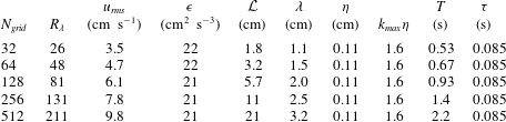
As suggested in the definition of (3.6), the largest turbulent eddies are expected to be important in the interaction with particles. In order to investigate this interaction, we use the same strategy as that used by Lanotte et al. (Reference Lanotte, Seminara and Toschi2009). Their DNS fixed the turbulence statistics of the smallest eddies, and expanded the number of grids, the domain size and the sizes of the largest eddies to focus on the interaction between the largest eddies and cloud droplets by condensation–evaporation. Turbulence statistics for our DNS without particles are summarized in table 1. Note that these statistics are changed under the effect of particles due to the turbulence modulation by particles.
Mean turbulence parameters for cases without particles. In the table,
 $N_{grid}$
is the number of grid points in physical space for each direction,
 $R_{\unicode[STIX]{x1D706}}$
is the Taylor microscale Reynolds number,
 $u_{rms}$
is the RMS velocity,
 $\unicode[STIX]{x1D716}$
is the mean energy dissipation rate per unit mass,
 ${\mathcal{L}}$
is the integral scale,
 $\unicode[STIX]{x1D706}$
is the Taylor microscale,
 $\unicode[STIX]{x1D702}$
is the Kolmogorov length,
 $k_{max}\unicode[STIX]{x1D702}$
is the cutoff wavenumber normalized by the Kolmogorov length,
 $T$
is the large-eddy turnover time, and
 $\unicode[STIX]{x1D70F}$
is the Kolmogorov time. The grid length is
 $\unicode[STIX]{x0394}x=2~\text{mm}$
and the domain size is
 $L_{box}=N_{grid}\unicode[STIX]{x0394}x$
.

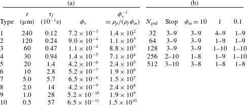
(a) Type of particle parameter. Columns from left to right are the type number, the particle radius
 $r$
, the flow relaxation time
 $\unicode[STIX]{x1D70F}_{f}$
, the volume fraction
 $\unicode[STIX]{x1D719}_{v}$
, and
 $\unicode[STIX]{x1D719}_{v}^{-1}$
, corresponding to the particle-to-fluid density ratio divided by the mass-loading parameter
 $\unicode[STIX]{x1D70C}_{p}/(\unicode[STIX]{x1D70C}_{f}\unicode[STIX]{x1D719}_{m})$
(see (3.5)). The inertial response time is given by
 $\unicode[STIX]{x1D70F}_{p}=\unicode[STIX]{x1D70F}_{f}\unicode[STIX]{x1D719}_{m}$
for cases with moving particles (
 $\unicode[STIX]{x1D719}_{m}=10$
, 1 and 0.1). These 10 types of experiment were conducted changing the grid number
 $N_{grid}$
and the mass-loading parameter
 $\unicode[STIX]{x1D719}_{m}$
. (b) The particle parameter used in each
 $N_{grid}$
and
 $\unicode[STIX]{x1D719}_{m}$
experiment is summarized according to type number. The column ‘Stop’ indicates the experiment with particles fixed in space. For example, for the
 $\unicode[STIX]{x1D719}_{m}=10$
and
 $N_{grid}=512$
experiment, parameters with type numbers 3 through 8 in part (a) of table are used.

The total number of particles in the domain is the same as the total number of grid points
 $N_{grid}^{3}$
, corresponding to the number density
 $n_{p}=125~\text{cm}^{-3}$
with the grid length
 $\unicode[STIX]{x0394}x=2~\text{mm}$
. Particles are mono-dispersed and have a radius of
 $r$
. We conducted four kinds of experiment. In the first case, we fixed the positions of all particles in space after distributing their initial positions uniformly and randomly in the domain. In the other three cases, we let particles move according to (2.1) and (2.2), with
 $\unicode[STIX]{x1D719}_{m}~\text{s}$
et to
 $10$
,
 $1$
and
 $0.1$
for each case. For each experiment with different
 $\unicode[STIX]{x1D719}_{m}$
and
 $N_{grid}$
, we explored 10 combinations of parameters by changing the density of particle
 $\unicode[STIX]{x1D70C}_{p}$
and the radius
 $r$
. These combinations of parameters, assigned numbers from 1 to 10 for convenience, are summarized in table 2(a). The combination of parameters used for each experiment is summarized in table 2(b). Note that the volume fraction
 $\unicode[STIX]{x1D719}_{v}$
for the present DNS is generally smaller than
 $10^{-3}$
, as shown in table 2(a), and, accordingly, the suspension can be assumed to be dilute (Elghobashi Reference Elghobashi1994).
4.2 Results
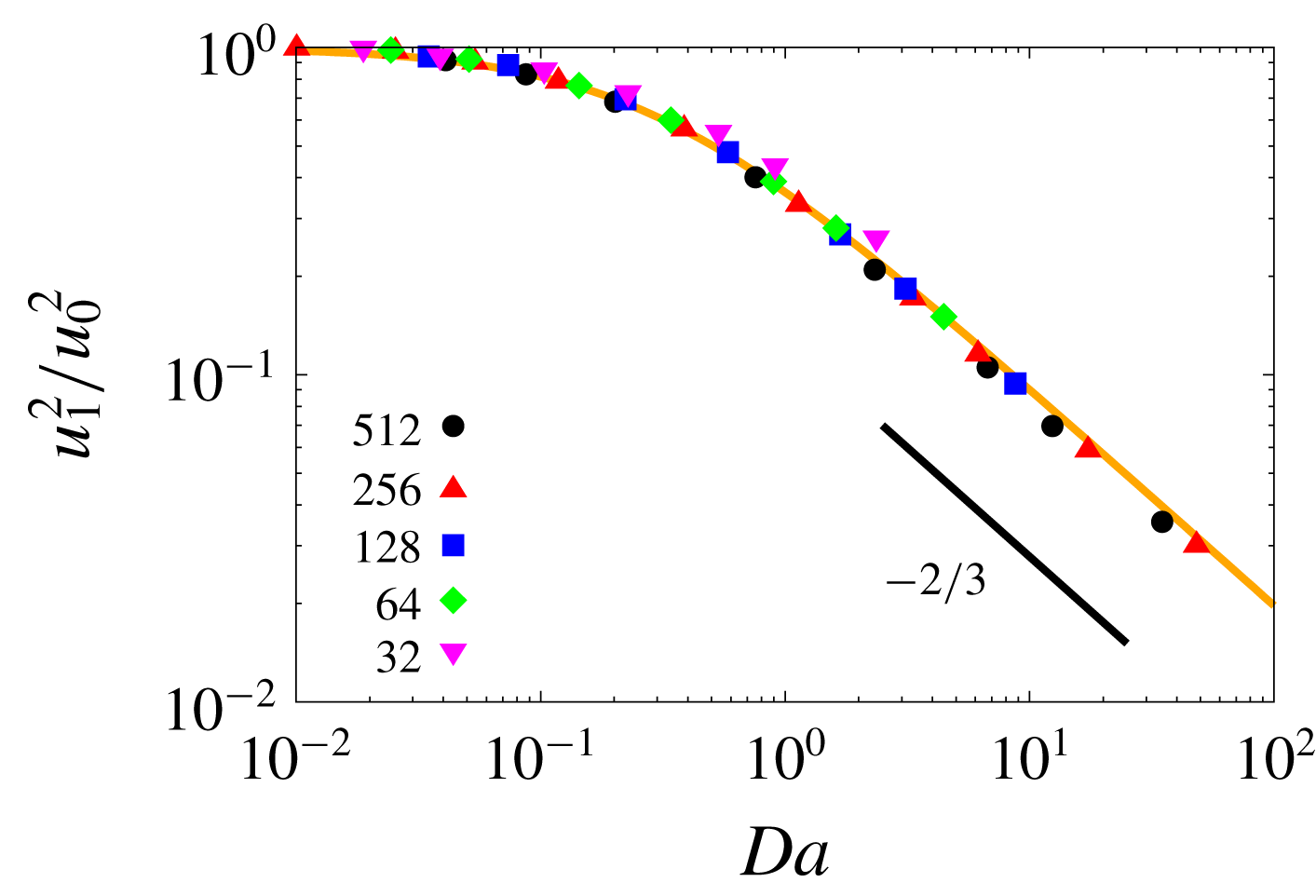
The ratio
 $u_{1}^{2}/u_{0}^{2}$
for the cases with particles fixed in space, where
 $u_{0}$
and
 $u_{1}$
are the RMS velocity of turbulence without and with particles, respectively. The horizontal axis is the Damköhler number
 $Da=T_{1}/\unicode[STIX]{x1D70F}_{f}$
, where
 $T_{1}$
is the large-eddy turnover time for turbulence under the effect of particles. The orange curve indicates the theoretical prediction (3.10) with
 $c=3.61$
. The short black line indicates the slope
 $-2/3$
expected for
 $Da\gg 1$
from (3.10).

We first investigate the results of DNS with particles fixed in space. Figure 1 shows the ratio
 $u_{1}^{2}/u_{0}^{2}$
, where
 $u_{0}$
and
 $u_{1}$
are the RMS velocity of fluid turbulence without and with the effect of particles, respectively. The horizontal axis is
 $Da=T_{1}/\unicode[STIX]{x1D70F}_{f}$
, the Damköhler number in terms of the large-eddy turnover time for turbulence under the effect of particles. The theoretical prediction (3.10) with
 $c=3.61$
is indicated by the orange curve, onto which all experimental results perfectly collapse. The Damköhler number is an index of the turbulence modulation by particles, where the modulation is significant for
 $Da\gg 1$
, while the modulation is not significant for
 $Da\ll 1$
. The slope of the curve is close to
 $-2/3$
for
 $Da>1$
in figure 1, indicating that the turbulent kinetic energy is dissipated mainly by particles in this range.
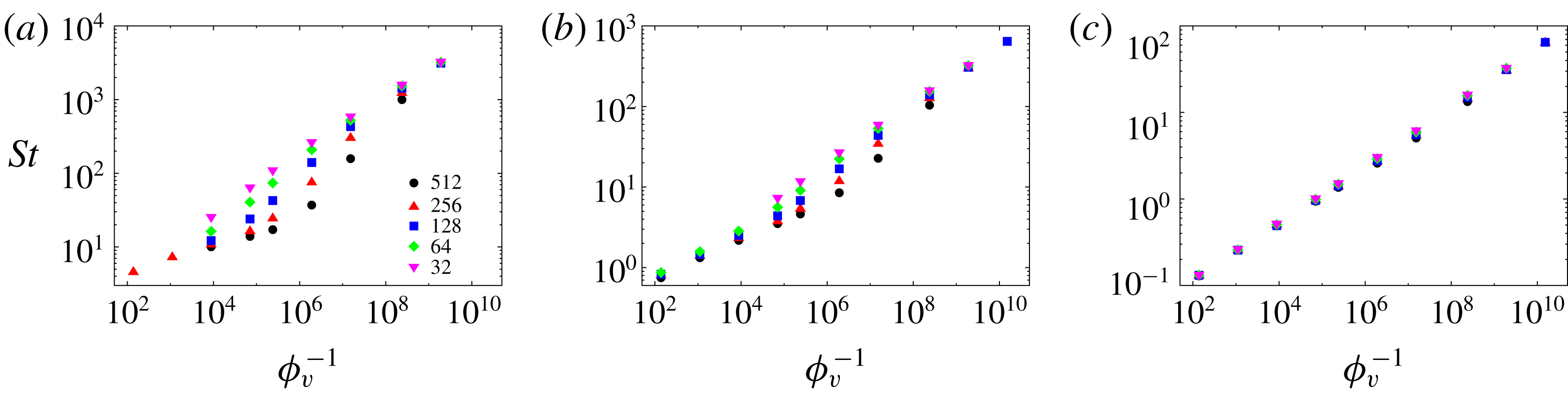
Stokes number
 $St=\unicode[STIX]{x1D70F}_{p}/\unicode[STIX]{x1D70F}_{1}$
of the experiments with
 $\unicode[STIX]{x1D719}_{m}=10$
,
 $1$
and
 $0.1$
for panels (a), (b) and (c), respectively. Here,
 $\unicode[STIX]{x1D70F}_{1}$
is the Kolmogorov time for turbulence under the effect of particles and the horizontal axis is
 $\unicode[STIX]{x1D719}_{v}^{-1}=\unicode[STIX]{x1D70C}_{p}/(\unicode[STIX]{x1D70C}_{f}\unicode[STIX]{x1D719}_{m})$
in table 2(a). Note the difference in the vertical axis.

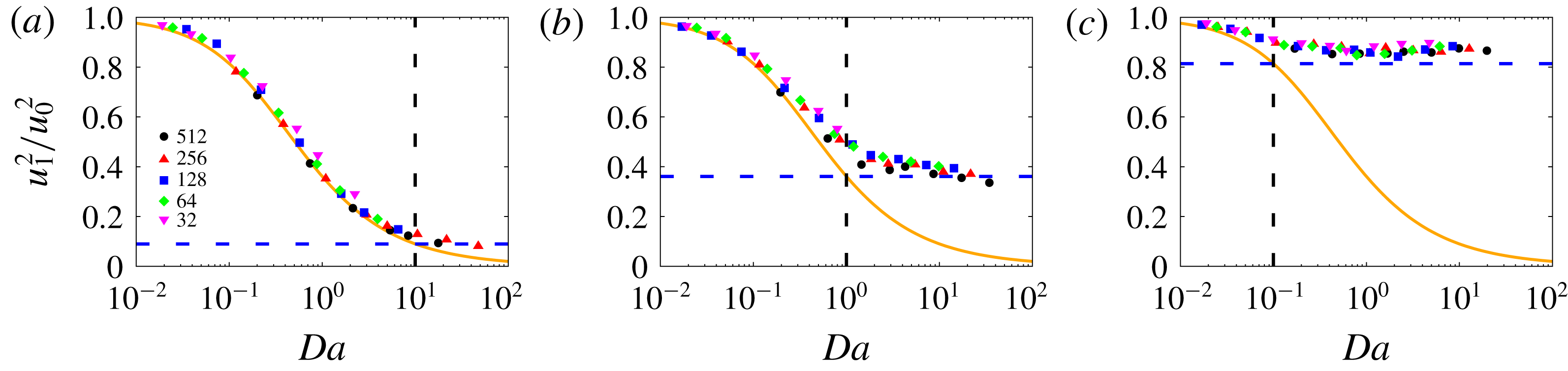
Same as figure 1, except that particles are moving and the mass-loading parameters are
 $\unicode[STIX]{x1D719}_{m}=10$
,
 $1$
and
 $0.1$
for panels (a), (b) and (c), respectively. Note that the vertical axis is linear. The vertical dashed line in each panel indicates the point where the Damköhler number is equal to the mass-loading parameter for each experiment (i.e.
 $Da=10$
, 1 and 0.1 for (a), (b) and (c), respectively). The horizontal dashed line in each panel indicates the value obtained by substituting
 $Da=\unicode[STIX]{x1D719}_{m}$
into (3.10) for each experiment.

We next consider the results of DNS with moving particles. Figures 2(a) through 2(c) summarize the Stokes number
 $St=\unicode[STIX]{x1D70F}_{p}/\unicode[STIX]{x1D70F}_{1}$
for each experiment, where
 $\unicode[STIX]{x1D70F}_{1}$
is the Kolmogorov time for turbulence under the effect of particles.
Figures 3(a) through 3(c) are the same as figure 1, except that particles are moving and the mass-loading parameters are
 $\unicode[STIX]{x1D719}_{m}=10$
,
 $1$
and 0.1, respectively. Note that the vertical axis is linear. The vertical dashed line in each panel indicates the point where the Damköhler number is equal to the mass-loading parameter for each experiment (i.e.
 $Da=10$
, 1 and 0.1 for figures 3(a) through 3(c), respectively). Namely, from (3.5) and (3.6), the large-eddy turnover time
 $T_{1}$
is shorter/longer than the inertial response time
 $\unicode[STIX]{x1D70F}_{p}$
on the left/right-hand sides of the dashed line, respectively. In each panel, all results collapse well onto a single curve, but the shape of the curve is different in each panel. Experimental results approximately follow the orange curve [for particles fixed in space, (3.10)] for
 $Da<\unicode[STIX]{x1D719}_{m}$
and start to deviate from the orange curve for
 $Da\sim \unicode[STIX]{x1D719}_{m}$
. For
 $Da>\unicode[STIX]{x1D719}_{m}$
, the ratio
 $u_{1}^{2}/u_{0}^{2}$
apparently becomes insensitive to
 $Da$
– especially in figure 3(c). These results suggest that the ratio
 $u_{1}^{2}/u_{0}^{2}$
, or turbulence modulation by particles with a fixed mass-loading parameter, can be expressed by a certain universal function of the Damköhler number. The horizontal dashed line in each panel in figure 3 indicates the value obtained by substituting
 $Da=\unicode[STIX]{x1D719}_{m}$
into (3.10) for each experiment. Despite its simplicity, this estimation can predict fairly well the level of the plateau for
 $Da>\unicode[STIX]{x1D719}_{m}$
in each panel.
The physical interpretation for the dependence on the Damköhler number is as follows. For
 $Da<\unicode[STIX]{x1D719}_{m}$
, even the time scale of the largest eddies in turbulence is shorter than the inertial response time of particles (
 $T_{1}<\unicode[STIX]{x1D70F}_{p}$
). Particles are sufficiently heavy, so that turbulent eddies of all sizes feel as if these particles are unmoving obstacles. Therefore, the ratio
 $u_{1}^{2}/u_{0}^{2}$
follows the theoretical curve (3.10) for stopped particles. On the other hand, for
 $Da>\unicode[STIX]{x1D719}_{m}$
, the time scale of the largest eddies is longer than the inertial response time (
 $T_{1}>\unicode[STIX]{x1D70F}_{p}$
). For
 $Da\gg \unicode[STIX]{x1D719}_{m}$
, the inertial response time of particles is sufficiently short, so that these particles are like passive tracers for the largest eddies – hence the limited turbulence modulation in this parameter range.
5 Conclusion
In the present study, we introduced a new time scale for turbulence modulation by particles. The new time scale is inversely proportional to the particle number density and the particle radius, and can be regarded as a counterpart of the phase relaxation time, which is an important time scale in cloud physics characterizing the interaction between turbulence and cloud droplets by condensation–evaporation. Based on this similarity, the new time scale is referred to as the flow relaxation time. We developed a simple scaling argument for the case in which particles are uniformly randomly distributed in the domain with their positions fixed in space, and derived an analytical estimate for turbulence modulation by particles as in (3.10). This predicts that the ratio
 $u_{1}^{2}/u_{0}^{2}$
is controlled by the Damköhler number
 $Da$
, which is defined as the ratio of the turbulence large-eddy turnover time to the flow relaxation time.
We conducted the DNS of particles in turbulence and confirmed that the prediction (3.10) actually holds when particles are fixed in space. We also conducted the DNS with moving particles for three cases of the mass-loading parameter (
 $\unicode[STIX]{x1D719}_{m}=10$
,
 $1$
and
 $0.1$
). We demonstrated that, for each case of
 $\unicode[STIX]{x1D719}_{m}$
, the ratio
 $u_{1}^{2}/u_{0}^{2}$
collapses well onto a single curve when arranged in terms of
 $Da$
, suggesting that the ratio
 $u_{1}^{2}/u_{0}^{2}$
can be expressed by a certain universal function of the Damköhler number and the mass-loading parameter. The shape of the curve is different for each
 $\unicode[STIX]{x1D719}_{m}$
experiment. For
 $Da<\unicode[STIX]{x1D719}_{m}$
, the curve follows the theoretical curve for particles at rest (3.10), but starts to deviate from the theoretical curve for
 $Da\sim \unicode[STIX]{x1D719}_{m}$
. For
 $Da>\unicode[STIX]{x1D719}_{m}$
, the ratio
 $u_{1}^{2}/u_{0}^{2}$
is apparently insensitive to
 $Da$
. We provided a physical interpretation for this dependence.
Since the present study demonstrated the importance of the Damköhler number, here we briefly mention two examples of
 $Da$
for the particle-laden turbulent flow. The first example is water droplets in the atmospheric clouds. Using typical parameters
 $\unicode[STIX]{x1D708}=0.15~\text{cm}^{2}~\text{s}^{-1}$
,
 $n_{p}=100~\text{cm}^{-3}$
,
 $r=10^{-3}~\text{cm}$
and
 $T>10^{2}~\text{s}$
, we have
 $\unicode[STIX]{x1D70F}_{f}=(6\unicode[STIX]{x03C0}\unicode[STIX]{x1D708}n_{p}r)^{-1}=3.5~\text{s}$
and
 $Da=T/\unicode[STIX]{x1D70F}_{f}>30$
. Since the mass-loading parameter found in clouds is at most
 $\unicode[STIX]{x1D719}_{m}=0.01$
(Vaillancourt & Yau Reference Vaillancourt and Yau2000), which is much smaller than
 $Da$
, the ratio
 $u_{1}^{2}/u_{0}^{2}$
can be estimated by substituting
 $\unicode[STIX]{x1D719}_{m}$
into (3.10), which gives
 $[1+3.61\times (0.01)]^{-2/3}=0.98$
. The turbulent kinetic energy is expected to be reduced only by 2 %, which is negligible. This supports the validity of the one-way coupling approximation usually assumed in DNS of cloud turbulence (Vaillancourt, Yau & Grabowski Reference Vaillancourt, Yau and Grabowski2001). The second example is the laboratory chamber experiment of particle-laden turbulent air flow by Tanaka & Eaton (Reference Tanaka and Eaton2010). Based on the assumption of isotropy, and using their turbulence parameter
 $R_{\unicode[STIX]{x1D706}}=130$
,
 $\unicode[STIX]{x1D702}=1.1\times 10^{-4}$
m and
 $u_{rms}\sim 1$
m s
 $^{-1}$
, the integral scale is estimated as
 ${\mathcal{L}}\sim 0.02$
m (Tennekes & Lumley Reference Tennekes and Lumley1972), and the large-eddy turnover time is
 $T\sim {\mathcal{L}}/u_{rms}=0.02~\text{s}$
. If we use the parameter for the experiment with glass particles (diameter
 $d_{p}=250$
 $\unicode[STIX]{x03BC}$
m and
 $\unicode[STIX]{x1D719}_{m}=0.41$
),
 $\unicode[STIX]{x1D70F}_{f}=\unicode[STIX]{x1D70F}_{p}/\unicode[STIX]{x1D719}_{m}\sim 0.5~\text{s}$
. From these estimations, we have
 $Da=T/\unicode[STIX]{x1D70F}_{f}\sim 0.04$
. Since
 $Da$
is sufficiently smaller than
 $\unicode[STIX]{x1D719}_{m}$
, we can use (3.10). The ratio
 $u_{1}^{2}/u_{0}^{2}$
is roughly estimated as
 $[1+3.61\times (0.04)]^{-2/3}=0.9$
. The turbulent kinetic energy is expected to be reduced by 10 %. Although this estimation is smaller than the measured reduction of 25 % (Tanaka & Eaton Reference Tanaka and Eaton2010), the agreement is not bad, given the uncertainty of the turbulence parameters for large scales.
Finally, we note the consistency of the results obtained in the present study and in the previous studies. Turbulence modulation by particles in various systems is reviewed in § 6 of Balachandar & Eaton (Reference Balachandar and Eaton2010). For jet and pipe flows, turbulence is augmented when particles are larger than approximately 1/10th of the integral scale, whereas turbulence is attenuated by smaller particles (Gore & Crowe Reference Gore and Crowe1991). Similar trends are also reported for fully developed channel flow, where the turbulent intensity is enhanced by particles larger than the Kolmogorov length but is reduced by smaller particles (Kulick, Fessler & Eaton Reference Kulick, Fessler and Eaton1994; Paris & Eaton Reference Paris and Eaton2001; Kussin & Sommerfeld Reference Kussin and Sommerfeld2002). On the other hand, for forced isotropic turbulence, DNS of the two-way coupling between particles and turbulence showed that the turbulent intensity is always reduced by particles (Squires & Eaton Reference Squires and Eaton1993; Boivin, Simonin & Squires Reference Boivin, Simonin and Squires1998). The results of the present study are consistent with these previous studies, since we considered forced isotropic turbulence and confirmed that turbulence is always attenuated by particles as shown in figure 3.
Acknowledgements
We are grateful to Professor Raymond Shaw for fruitful discussions and instructive comments. The term flow relaxation time was proposed by Professor Shaw for the time scale
 $\unicode[STIX]{x1D70F}_{f}$
. We are also grateful to three anonymous reviewers for many useful comments. This research used computational resources of the K computer provided by the RIKEN Center for Computational Science through the HPCI System Research project (Project ID: hp180070, hp190043). The computational support provided by the Japan High Performance Computing and Networking, Large-scale Data Analyzing and Information Systems (JHPCN) (jh180009, jh190018), the High Performance Computing (HPC 2018, 2019) at Nagoya University, and the Earth Simulator supercomputer system operated by the Japan Agency for Marine-Earth Science and Technology (JAMSTEC) are also gratefully acknowledged. The present study was supported by MEXT KAKENHI through grant no. 15H02218 and JSPS KAKENHI grants no. 18K03925 and no. 18K13611.