

Introduction
American states do not make policy in isolation. When one state adopts a new education reform, neighboring states take notice, professional networks transmit information about the design and performance of the policy, and the cumulative pattern of adoption creates pressure on remaining holdouts (Berry and Berry Reference Berry and Berry1990; Walker Reference Walker1969). This interstate interdependence is a defining feature of American federalism: the 50-state system functions as a policy laboratory precisely because states observe, learn from, compete with, and emulate one another (Shipan and Volden Reference Shipan and Volden2008). Understanding the channels through which states influence each other in policymaking is a central question for scholars of state politics.
This study examines two such channels and how their relative importance has evolved. A channel of influence is defined as a structural pathway along which adoption-relevant information may travel between jurisdictions, distinct from the cognitive or strategic mechanisms (learning, imitation, emulation, competition) that operate within those channels. The geographic channel runs through shared borders, regional media markets, and regional cooperative-federalism infrastructure; the network channel runs through inferred policy-pathway ties that need not coincide with geography (Desmarais, Harden, and Boehmke Reference Desmarais, Harden and Boehmke2015; Mallinson Reference Mallinson2021b). Disentangling these channels within a unified empirical framework, while remaining transparent about the limits of channel-level evidence for adjudicating among micro-mechanisms, motivates the analysis.
The empirical task is complicated by two recurring methodological concerns. One is the choice between contemporaneous and temporally lagged spatial specifications. The standard spatial autoregressive (SAR) model implies simultaneous spatial determination of adoption outcomes; the spatial-X (SLX) model implies sequential adoption in which a state observes prior neighbor decisions before its own. SLX is adopted as the primary specification for the 10 education policies analyzed below because their multi-decade diffusion windows are well-described by sequential observation. The spatial Durbin model (SDM) results reported in the “Spatial Durbin model: scope conditions for SAR and SLX specifications” section show empirically that contemporaneous (SAR) determination dominates for rapid-diffusion policies (Military Children Compact, Student Borrowing Capacity Act, School Choice; all diffusing in fewer than seven years), while lagged (SLX) determination dominates for sequential-diffusion policies. The choice between SAR and SLX is therefore a substantive specification decision governed by the temporal structure of the diffusion process under study, not a universal methodological ranking.
Another methodological concern is the construction of the network variable. If the policy-similarity network used to predict adoption is itself constructed from the same adoption series being predicted, the network exposure measure partially re-encodes the dependent variable, inflating apparent network effects. The present analysis addresses this by constructing the primary policy-pathway network from the 714 non-education policies in SPID v1.2 (Boehmke et al. Reference Boehmke, Brockway, Desmarais, Harden, LaCombe, Linder and Wallach2020). Specification A is conceptually similar to the persistent-policy-pathways measure of Desmarais, Harden, and Boehmke (Reference Desmarais, Harden and Boehmke2015) distributed with State Policy Innovation and Diffusion (SPID); the analysis uses a Jaccard-based exogenous network rather than the published persistent-pathways measure because the latter requires inputs (specific time-window choices and latent-variable estimation parameters) that cannot be fully reproduced from the SPID v1.2 distribution alone. The substantive direction of the network finding is robust across both operationalizations. Under the exogenous specification, the network coefficient is approximately 1.7 in the fixed-effects Full model and 0.85 with policy-level random intercepts. The coefficient remains positive and statistically significant, indicating that a genuine relational channel exists alongside but distinct from inflation due to within-domain endogeneity.
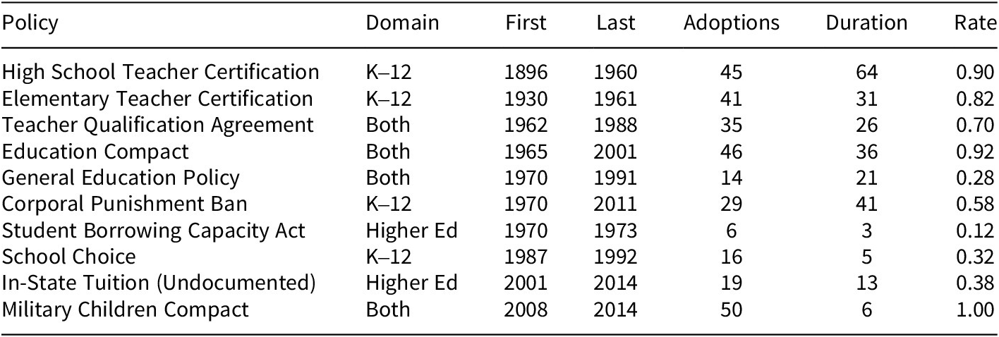
The framework is applied to 10 education policies adopted across the 50 American states between 1896 and 2017, drawn from SPID v1.2. The 10 policies span K-12 and higher-education governance and provide adoption windows ranging from three years (Student Borrowing Capacity Act) to 64 years (High School Teacher Certification), enabling within-sample comparison across policy domains, historical periods, and adoption scopes. Table 1 lists the policies.
Education policies analyzed (N = 10)

Table 1. Long description
The table contains seven columns: Policy, Domain, First (year), Last (year), Adoptions, Duration, and Rate.
* High School Teacher Certification: K through 12 domain, 1896 to 1960, 45 adoptions, 64-year duration, 0.90 rate.
* Elementary Teacher Certification: K through 12 domain, 1930 to 1961, 41 adoptions, 31-year duration, 0.82 rate.
* Teacher Qualification Agreement: Both domains, 1962 to 1988, 35 adoptions, 26-year duration, 0.70 rate.
* Education Compact: Both domains, 1965 to 2001, 46 adoptions, 36-year duration, 0.92 rate.
* General Education Policy: Both domains, 1970 to 1991, 14 adoptions, 21-year duration, 0.28 rate.
* Corporal Punishment Ban: K through 12 domain, 1970 to 2011, 29 adoptions, 41-year duration, 0.58 rate.
* Student Borrowing Capacity Act: Higher Ed domain, 1970 to 1973, 6 adoptions, 3-year duration, 0.12 rate.
* School Choice: K through 12 domain, 1987 to 1992, 16 adoptions, 5-year duration, 0.32 rate.
* In-State Tuition (Undocumented): Higher Ed domain, 2001 to 2014, 19 adoptions, 13-year duration, 0.38 rate.
* Military Children Compact: Both domains, 2008 to 2014, 50 adoptions, 6-year duration, 1.00 rate.
Note: Ten education policies drawn from the State Policy Innovation and Diffusion (SPID) database, version 1.2. Adoption rate = total adoptions/50 states. Duration in years.
Three substantive patterns emerge from the analysis. Both geographic proximity and network exposure independently predict state adoption decisions, with each channel operating through institutionally distinct pathways even after controls for confounding state-level characteristics. The relative importance of these channels has shifted across historical periods: policies whose diffusion windows opened before the consolidation of nationally organized interstate policy infrastructure show predominantly spatial diffusion patterns, while policies entering their diffusion windows during the network-rich post-1970 environment exhibit a different mix in which network exposure carries more of the explanatory weight. The shift is robust across alternative network constructions, alternative era cut-points, and the addition of policy-level random intercepts. The contrast across policy domains is similarly informative: K-12 policies, governed through regional compact infrastructure, sustain a detectable spatial channel into the late twentieth century, while higher-education policies, governed through nationally organized accreditation and disciplinary networks, show a different pattern qualified by limited statistical power in the available higher-education subsample.
These findings carry three contributions. They demonstrate that the channels through which American states influence each other in education policymaking have shifted from geography-dominated to network-mediated pathways across the past century, consistent with the post-1965 institutional consolidation of nationally organized interstate policy bodies (Makse and Volden Reference Makse and Volden2011; Mallinson Reference Mallinson2021b). They show that the governance architecture of a policy domain conditions which channels are active, with K-12 governance, embedded in regionally bounded compact infrastructure, sustaining the geographic channel longer than higher-education governance, organized through national accreditation and disciplinary networks. They clarify that the choice between SAR and SLX is a substantive specification decision driven by whether the data-generating process involves sequential or contemporaneous influence, supported by direct empirical evidence in the SDM analysis.
The argument develops in five further sections. The “Theoretical framework” section establishes the theoretical framework that distinguishes channels of influence from the cognitive mechanisms operating within those channels, locates the present analysis in the literatures on policy diffusion and spatial econometrics, and develops four hypotheses. The “Data and methods” section describes the SPID v1.2 data, the construction of the spatial and network exposure measures, and the analytical strategy. The “Results” section reports the empirical results across eight specifications, including a SPID-wide methodological replication. The “Discussion” section discusses the substantive and methodological implications. The “Conclusion” section provides concluding remarks.
Theoretical framework
From mechanisms to channels
Theoretical accounts of policy diffusion converge on four primary mechanisms through which adoption in one jurisdiction affects adoption probabilities in others: learning, competition, emulation, and coercion (Dobbin, Simmons, and Garrett Reference Dobbin, Simmons and Garrett2007; Shipan and Volden Reference Shipan and Volden2008, Reference Shipan and Volden2012). The four-mechanism typology has organized the field for two decades and has informed both quantitative event-history analyses (Berry and Berry Reference Berry and Berry1990; Boehmke Reference Boehmke2009) and qualitative process-tracing investigations (Karch Reference Karch2007; Mallinson Reference Mallinson2020).
Learning involves rational assessment of policy performance in other jurisdictions, with decision-makers updating their beliefs on the basis of observed outcomes (Gilardi Reference Gilardi2010; Volden, Ting, and Carpenter Reference Volden, Ting and Carpenter2008). The formal model developed by Volden, Ting, and Carpenter (Reference Volden, Ting and Carpenter2008) shows that learning produces detectable diffusion patterns even when policy-makers in different jurisdictions hold heterogeneous priors and confront heterogeneous local conditions. Empirical work has documented learning effects in welfare reform (Volden Reference Volden2006), tax policy (Devereux, Lockwood, and Redoano Reference Devereux, Lockwood and Redoano2008), and health insurance regulation (Pacheco Reference Pacheco2012). The learning mechanism predicts that policy adoption will respond to evidence about how policies have performed elsewhere, with stronger responses to information from jurisdictions whose institutional and demographic characteristics resemble those of the focal state.
Competition drives diffusion when jurisdictions adopt policies to maintain or improve competitive positions (Brueckner Reference Brueckner2003). Competitive pressures arise when states share economic, demographic, or political environments such that the adoption of a policy in one jurisdiction creates incentives for adoption in others. Tax-base competition, regulatory competition, and competition for skilled labor or business location decisions are central examples. The competition mechanism predicts geographic clustering when jurisdictions in the same regional economic environment respond to the policy moves made by neighboring jurisdictions.
Emulation reflects adoption motivated by perceptions of legitimacy or appropriateness rather than by instrumental performance assessment (DiMaggio and Powell Reference DiMaggio and Powell1983). Emulation can produce diffusion patterns that are difficult to distinguish from learning in observational data, because both mechanisms generate adoption clustering around states viewed as reference points. Mallinson (Reference Mallinson2021b) shows that ideological alignment increasingly conditions which states serve as reference points for emulation, partially displacing the role of geographic proximity that earlier work had emphasized.
Coercion operates when higher-level authorities mandate or incentivize adoption (Shipan and Volden Reference Shipan and Volden2008). Federal grant conditions, court rulings interpreting constitutional requirements, and conditions attached to federal regulatory waivers each create top-down pressures that can produce diffusion patterns indistinguishable in event-history data from horizontal learning or emulation. Boehmke (Reference Boehmke2009) identifies a further analytical challenge: the distinction between policy emulation, in which states adopt a policy because other states have adopted it, and policy convergence, in which states adopt a policy because they share underlying conditions that generate independent adoption decisions.
These theoretical accounts of mechanism motivate why channel-level patterns of inter-state influence might be expected to appear in the data, but they do not license the stronger claim that channel-level patterns themselves identify the underlying mechanisms. The research design developed below identifies the channels through which inter-state influence travels and the institutional conditions under which different channels are active. It does not directly identify the cognitive or strategic mechanisms operating within those channels. Designs capable of identifying mechanisms include experimental manipulation of policy-relevant information (Butler et al. Reference Butler, Volden, Dynes and Shor2017), bill-text analysis distinguishing copying from independent drafting (Hansen and Jansa Reference Hansen and Jansa2021; Linder et al. Reference Linder, Desmarais, Burgess and Giraudy2020), and process-tracing of individual adoption events (Mallinson Reference Mallinson2020). The channel-level findings reported below complement, rather than substitute for, mechanism-level work, and the interpretation of channel-level patterns should remain modest about what the design can and cannot establish.
Spatial, network, and temporal channels
Network ties are operationalized as policy-pathway connections inferred from patterns of co-adoption across the State Policy Innovation and Diffusion database. The primary specification constructs these connections from the 714 SPID policies that exclude the 10 education policies analyzed in this study, so that the network is exogenous to the dependent variable. Network exposure for a state-policy-year is the proportion of pathway-network partners belonging to a given state that have already adopted the focal policy.
Geographic proximity affects diffusion through multiple pathways: shared media markets (Mitchell Reference Mitchell2018), regional labor mobility, participation in regional organizations and interstate compacts (Balla Reference Balla2001), and similar economic and demographic conditions (Case, Rosen, and Hines Reference Case, Rosen and Hines1993; Mooney Reference Mooney2001). The critical analytical question is whether observed geographic clustering reflects genuine spatial interdependence or spatially correlated confounders.
The use of SLX as the primary specification for the 10 education policies rests on a substantive judgment about the temporal structure of these diffusion processes. The 10 education policies have multi-decade adoption windows, and the diffusion theory governing them describes sequential observation in which a state observes what its neighbors did in the past and updates its own adoption probability accordingly (Berry and Berry Reference Berry and Berry1990). The SAR specification, by contrast, describes contemporaneous spatial determination, which is the appropriate model for rapid policy bandwagons (Boushey Reference Boushey2010), conformity-driven emulation under high media salience (Pacheco Reference Pacheco2012), and crisis-period clustering when multiple states convene under shared external pressure. As reported in the “Spatial Durbin model: scope conditions for SAR and SLX specifications” section, on subsamples of the 10 education policies divided by diffusion duration, the contemporaneous specification recovers a stronger spatial signal for the rapid-diffusion subset (those diffusing in fewer than seven years), while the lagged specification recovers a stronger signal for the sequential-diffusion subset. The SDM, which combines the SAR ρWy term with the SLX W*X*θ term, provides a joint specification for analysts who wish to test which process dominates.
Network position captures relational pathways that may or may not coincide with geography. States connected through professional associations, interstate compacts, or similar institutional configurations may exchange policy-relevant information regardless of physical proximity (Balla Reference Balla2001; Desmarais, Harden, and Boehmke Reference Desmarais, Harden and Boehmke2015; Volden Reference Volden2006). Mistur and Matisoff (Reference Mistur and Matisoff2024) demonstrate that stakeholder movement within policy networks serves as a concrete mechanism for cross-state policy transmission. Mallinson (Reference Mallinson2021b) shows that ideological alignment increasingly conditions which states serve as reference points for policy learning, partially displacing the role of geographic proximity. Parinandi, Langehennig, and Trautmann (Reference Parinandi, Langehennig and Trautmann2021) provide evidence that legislators attend to policy developments in other states through structured professional channels rather than through undifferentiated geographic exposure.
Temporal dynamics introduce path dependence and momentum effects that condition how spatial and network channels operate. The diffusion-life-course argument advanced by Mallinson (Reference Mallinson2021a) shows that the mechanisms driving early adoption differ from those sustaining later-stage diffusion. Mallinson and Jansa (Reference Mallinson and Jansa2026) show that conclusions about mechanism importance depend on the temporal window examined.
Hypotheses
These theoretical considerations generate four predictions. The opening pair anchors the integrated framework; the remaining two test conditional propositions about how channel importance varies across historical periods and policy domains.
The relative importance of geographic and network channels depends on the institutional infrastructure available for cross-state policy communication at the time a policy enters its diffusion window. Mid-twentieth-century interstate policy communication was overwhelmingly mediated by physical proximity. The institutional landscape changed substantially with the consolidation of nationally organized interstate bodies between 1965 and 1975, including the Education Commission of the States (1965), the reorganized National Conference of State Legislatures (1975), the National Governors Association policy programs (1970s), and the expanded policy infrastructure of the Council of Chief State School Officers. The diffusion-life-course argument advanced by Mallinson (Reference Mallinson2021a) suggests that the relative weight of channels should differ across policies entering their diffusion window before versus after this institutional consolidation.
The institutional architecture governing a policy domain similarly conditions which channels are active. K-12 education in the United States is governed primarily by state agencies whose interstate cooperation runs through explicitly geographic regional compact infrastructure: the Western Interstate Commission for Higher Education (1953), the Southern Regional Education Board (1948), the Midwestern Higher Education Compact (1991), and the New England Board of Higher Education (1955). Higher-education governance, by contrast, runs through nationally organized accrediting bodies, disciplinary professional associations, and federal funding administrators, all of which are explicitly a-geographic in their operational structure. Recent evidence on policy diffusion in the higher-education-adjacent space, including Karch and Cravens (Reference Karch and Cravens2014) on higher education performance funding, supports the prediction that higher-education policy diffusion responds more to national professional and competitive networks than to geographic proximity.
Hypothesis 1 (Spatial Channel): The temporally lagged proportion of contiguous neighbors having adopted a policy will be positively associated with adoption hazard, net of network exposure and temporal controls.
Hypothesis 2 (Network Channel): Network exposure, measured as the proportion of policy-pathway-network ties to prior adopters using a network constructed exogenously from non-education SPID policies, will be positively associated with adoption hazard, net of spatial proximity and temporal controls.
Hypothesis 3 (Temporal Shift): For policies entering their diffusion window before the consolidation of nationally organized interstate policy infrastructure (operationalized as a 1970 cut-point with sensitivity to 1965 and 1980), the spatial channel will be more strongly associated with adoption hazard than the network channel; this relationship will reverse for policies entering after this consolidation.
Hypothesis 4 (Domain Contingency): The spatial channel will be more strongly associated with adoption hazard for K-12 policies than for higher-education policies, reflecting the differential geographic structuring of K-12 versus higher-education governance institutions. The network channel is expected in both domains, subject to statistical power.
Data and methods
Data source and policy selection
This study uses SPID v1.2 (Boehmke et al. Reference Boehmke, Brockway, Desmarais, Harden, LaCombe, Linder and Wallach2020), which records adoption dates for 724 policies across all 50 American states from 1691 to 2017. SPID was constructed by aggregating policy-adoption records from previously published diffusion studies, supplemented by primary source verification, and represents the most extensive single resource for state policy diffusion analysis currently available. The temporal depth of SPID, extending across more than three centuries of policy adoption, makes it particularly suitable for testing hypotheses about historical change in diffusion patterns. The breadth of policy coverage, spanning environmental, criminal justice, health, education, taxation, and many other domains, supports both within-domain analyses of the type developed in this study and broader cross-domain methodological investigations.
Education-related policies were identified through keyword search of policy names and descriptions in the SPID v1.2 distribution. Search terms included variants of “education,” “school,” “teacher,” “student,” “university,” “college,” “academic,” and policy-specific terminology drawn from the substantive education-policy literature. Candidate policies were then reviewed individually to confirm their substantive education-policy character and to assign them to a domain category. The procedure yielded 10 education policies (listed in Table 1) with 301 total adoption events spanning 1896–2014. The 10 policies span K-12 education (four policies, 131 events: High School Teacher Certification, Elementary Teacher Certification, Corporal Punishment Ban, School Choice), higher education (two policies, 25 events: Student Borrowing Capacity Act, In-State Tuition for Undocumented Students), and cross-domain policies that affect both K-12 and higher-education governance (four policies, 145 events: Teacher Qualification Agreement, Education Compact, General Education Policy, Military Children Compact).
Domain assignment follows the substantive scope of each policy as documented in the SPID metadata and supplementary state-level legislative records. Policies that explicitly target K-12 schools, teachers, or students are coded as K-12; policies that explicitly target post-secondary institutions, college students, or higher-education governance are coded as higher education. Policies whose statutory scope addresses both K-12 and higher-education contexts are coded as cross-domain and are included in both K-12 and higher-education domain analyses where appropriate. The cross-domain category captures policies such as the Education Compact (which establishes interstate agreements covering both K-12 and higher-education matters) and the Teacher Qualification Agreement (which addresses teacher credentialing across primary, secondary, and post-secondary settings).
To address concerns about sample size for the methodological claims, the analysis reports a complementary SPID-wide replication of the SLX-versus-SAR comparison covering 635 policies and 17,628 adoption events (“SPID-wide methodological replication” section). The SPID-wide replication restricts attention to policies with at least five adoptions, which excludes 89 SPID policies with fewer than five adopting states and removes 195 adoption events. The remaining sample preserves 87.7% of all SPID policies and 98.9% of all adoption events, providing a robust base for methodological generalization while excluding policies with insufficient variation to support discrete-time survival modelling.
Variables and measurement
Dependent variable and survival panel
The dependent variable is a binary indicator of policy adoption, coded 1 in the year a state adopts a given policy and 0 otherwise. The discrete-time survival panel contains 13,112 state-policy-year observations with 301 adoption events.
Spatial lag (lagged and contemporaneous)
The temporally lagged spatial lag (used in SLX) measures the proportion of contiguous border-sharing neighbors that had adopted the policy by year t − 1. The contemporaneous spatial lag (used in SAR-style comparisons and in the SDM) measures the proportion of contiguous neighbors that have adopted by year t, excluding the focal state’s own adoption to avoid mechanical identity. The spatial weights matrix is constructed from state border contiguity, identifying 106 unique border pairs across the 48 contiguous states. Alaska and Hawaii are treated as spatial isolates.
Network exposure: three specifications
The analysis constructs three policy-network specifications, presented in escalating order of independence from the dependent variable. Specification A (primary) constructs the network from Jaccard similarity on the 714 non-education SPID policies, with edges defined at or above the median Jaccard value. The exogeneity of this specification is conceptually similar to the published persistent-policy-pathways measure of Desmarais, Harden, and Boehmke (Reference Desmarais, Harden and Boehmke2015) distributed with SPID; the present analysis uses a Jaccard-based exogenous network rather than the published persistent-pathways measure because the latter requires inputs (specific time-window choices and latent-variable estimation parameters) that cannot be fully reproduced from the SPID v1.2 distribution alone. Specification B (conservative) is identical to A but additionally requires at least 10 mutually adopted policies per edge. Specification C (transparency) is a within-education Jaccard, reported alongside the exogenous specifications to make explicit the consequences of constructing networks within the same policy domain that constitutes the dependent variable.
Network exposure is calculated for each state-policy-year observation as the proportion of network ties belonging to the focal state that connect to states having adopted the given policy by year t − 1. The dyadic correlation between the contiguity adjacency matrix and the Specification A network adjacency matrix is 0.23, indicating that some geographic structure is reflected in the policy-pathway network but that the two are far from collinear; a residualized network-exposure robustness analysis is reported in the “Domain comparison: K-12 versus higher education” section.
Temporal controls and centrality
Cumulative adoption proportion measures the fraction of all 50 states having adopted a given policy by year t − 1. Time since earliest adoption measures years elapsed since the earliest adoption of each policy. Geographic degree centrality and policy-network degree centrality are included as state-level covariates.
State-level controls and the regional-dummy compromise
Regional dummies serve as a proxy for unmeasured state-level heterogeneity in the main models, but this approach masks within-region variation in political culture, legislative professionalism, and fiscal capacity. Two responses follow. For the post-1960 portion of the panel where the relevant published data series exist, a state-innovation activity index is constructed from the cumulative count of non-education SPID policy adoptions per state-year, standardized. This is a within-data-source proxy for the underlying construct of differential propensity of states to adopt new policies, available across the entire 1896–2017 panel. The “Post-1960 robustness with state-innovation control” section reports this robustness specification on the post-1960 sample (9,260 observations, 215 events). Regional dummies are retained in the main models because the Berry, Ringquist, Fording, and Hanson (Reference Berry, Ringquist, Fording and Hanson1998) ideology scores begin in 1960 and the Squire (Reference Squire2017) legislative-professionalism index begins in 1979; restricting the analysis to post-1979 policies to enable both controls would eliminate three of the four pre-1970 era policies that anchor the test of Hypothesis 3. This trade-off is acknowledged explicitly in the “Channels versus mechanisms” section, and domain-specific historical political-culture measurement is identified as a priority for future work.
Analytical strategy
The analysis proceeds in five stages. The descriptive stage reports adoption patterns and computes Moran’s I spatial autocorrelation statistics. The SLX estimation stage fits discrete-time logistic survival models in an incremental sequence and compares them via AIC and BIC. The era-specific stage tests Hypothesis 3 by estimating separate models for pre-1970 and post-1970 policies, with sensitivity at 1965 and 1980. The domain-specific stage tests Hypothesis 4 with separate models for K-12 and higher-education policies. The robustness stage includes (a) policy-level random-intercept estimation, (b) the post-1960 specification with the state-innovation control, (c) residualized network-exposure analysis, and (d) the SDM on rapid- versus sequential-diffusion subsamples. A complementary SPID-wide replication is reported in the “SPID-wide methodological replication” section.
Results
Descriptive patterns and spatial autocorrelation
The 10 education policies, listed in Table 1, exhibit substantial variation in adoption scope and timing. The Military Children Compact achieved universal adoption across all 50 states within six years (2008–2014); the Student Borrowing Capacity Act was adopted by only six states within three years (1970–1973). The mean diffusion duration is 24 years; duration ranges from 3 to 64 years. The two policies with the longest diffusion windows, High School Teacher Certification (1896–1960, 64 years) and Elementary Teacher Certification (1930–1961, 31 years), both achieved adoption rates above 80% of the 50-state universe; the policy with the shortest diffusion window that achieved universal adoption, the Military Children Compact, did so during a six-year period of intense interstate-compact activity coordinated through the Council of State Governments and the Department of Defense. The variability in diffusion tempo across the 10 policies provides analytical leverage for testing hypotheses about how channels of influence operate across different temporal structures of adoption.
Adoption scope varies systematically across policy domains. The four K-12 policies achieved a mean adoption rate of 0.66; the two higher-education policies achieved a mean adoption rate of 0.25. The cross-domain policies, which include both the Military Children Compact and the broader Education Compact, achieved the highest mean adoption rate of 0.73. The contrast in adoption rates between K-12 and higher-education policies is consistent with the institutional argument that K-12 governance, embedded in widely shared regional compact infrastructure, generates pressures for broad adoption, whereas higher-education governance, embedded in selective national accreditation and disciplinary networks, generates more selective adoption patterns conditioned by specific state circumstances.
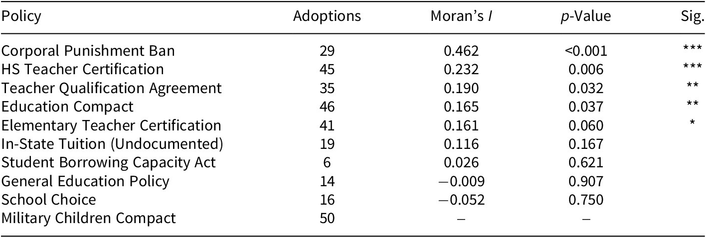
Moran’s I statistics calculated on the row-standardized contiguity matrix (Table 2) show positive spatial autocorrelation for older, K-12-oriented policies (Corporal Punishment Ban I = 0.46, p < 0.001; HS Teacher Certification I = 0.23, p = 0.006; Teacher Qualification Agreement I = 0.19, p = 0.032; Education Compact I = 0.17, p = 0.037; Elementary Teacher Certification I = 0.16, p = 0.060) and near-zero or negative autocorrelation for higher-education and recent policies (In-State Tuition I = 0.12, p = 0.167; Student Borrowing Capacity Act I = 0.03, p = 0.621; General Education Policy I = −0.01, p = 0.907; School Choice I = −0.05, p = 0.750). The Military Children Compact has zero variance because of universal adoption and therefore cannot be evaluated through Moran’s I. The pattern in Table 2 foreshadows the model-based finding of a temporal shift in channel importance: the spatial channel that produced detectable autocorrelation in pre-1970 policies has weakened or disappeared in more recent policies, even before introducing the multivariate framework that explicitly compares spatial and network channels.
Spatial autocorrelation by policy (Moran’s I, row-standardized contiguity)

Table 2. Long description
The table contains five columns: Policy, Adoptions, Moran’s I, p-Value, and Sig. (Significance).
* Corporal Punishment Ban: 29 adoptions, Moran’s I 0.462, p-Value less than 0.001, Sig. ***.
* H S Teacher Certification: 45 adoptions, Moran’s I 0.232, p-Value 0.006, Sig. ***.
* Teacher Qualification Agreement: 35 adoptions, Moran’s I 0.190, p-Value 0.032, Sig. **.
* Education Compact: 46 adoptions, Moran’s I 0.165, p-Value 0.037, Sig. **.
* Elementary Teacher Certification: 41 adoptions, Moran’s I 0.161, p-Value 0.060, Sig. *.
* In-State Tuition (Undocumented): 19 adoptions, Moran’s I 0.116, p-Value 0.167, Sig. none.
* Student Borrowing Capacity Act: 6 adoptions, Moran’s I 0.026, p-Value 0.621, Sig. none.
* General Education Policy: 14 adoptions, Moran’s I minus 0.009, p-Value 0.907, Sig. none.
* School Choice: 16 adoptions, Moran’s I minus 0.052, p-Value 0.750, Sig. none.
* Military Children Compact: 50 adoptions, Moran’s I and p-Value are not applicable due to universal adoption.
Note: Significance levels are defined as * p less than 0.10, ** p less than 0.05, and *** p less than 0.01.
Note: Row-standardized contiguity weights with 106 unique border pairs. The Military Children Compact has zero variance because of universal adoption and cannot be evaluated through Moran’s I. Stronger spatial autocorrelation appears for older, K-12-oriented policies that diffused before 1970. *p < 0.10. **p < 0.05. ***p < 0.01.
Main models: spatial and network channels
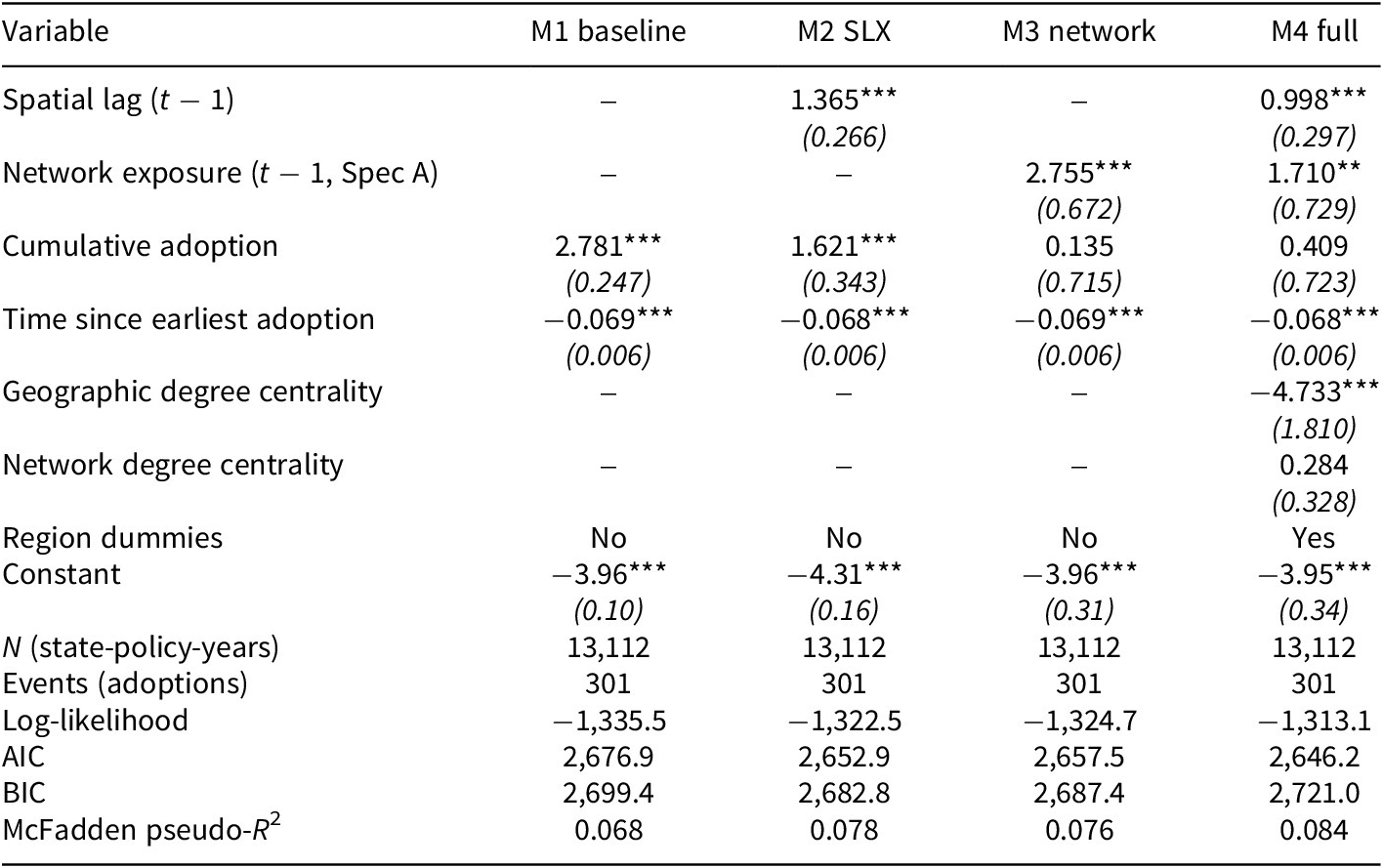
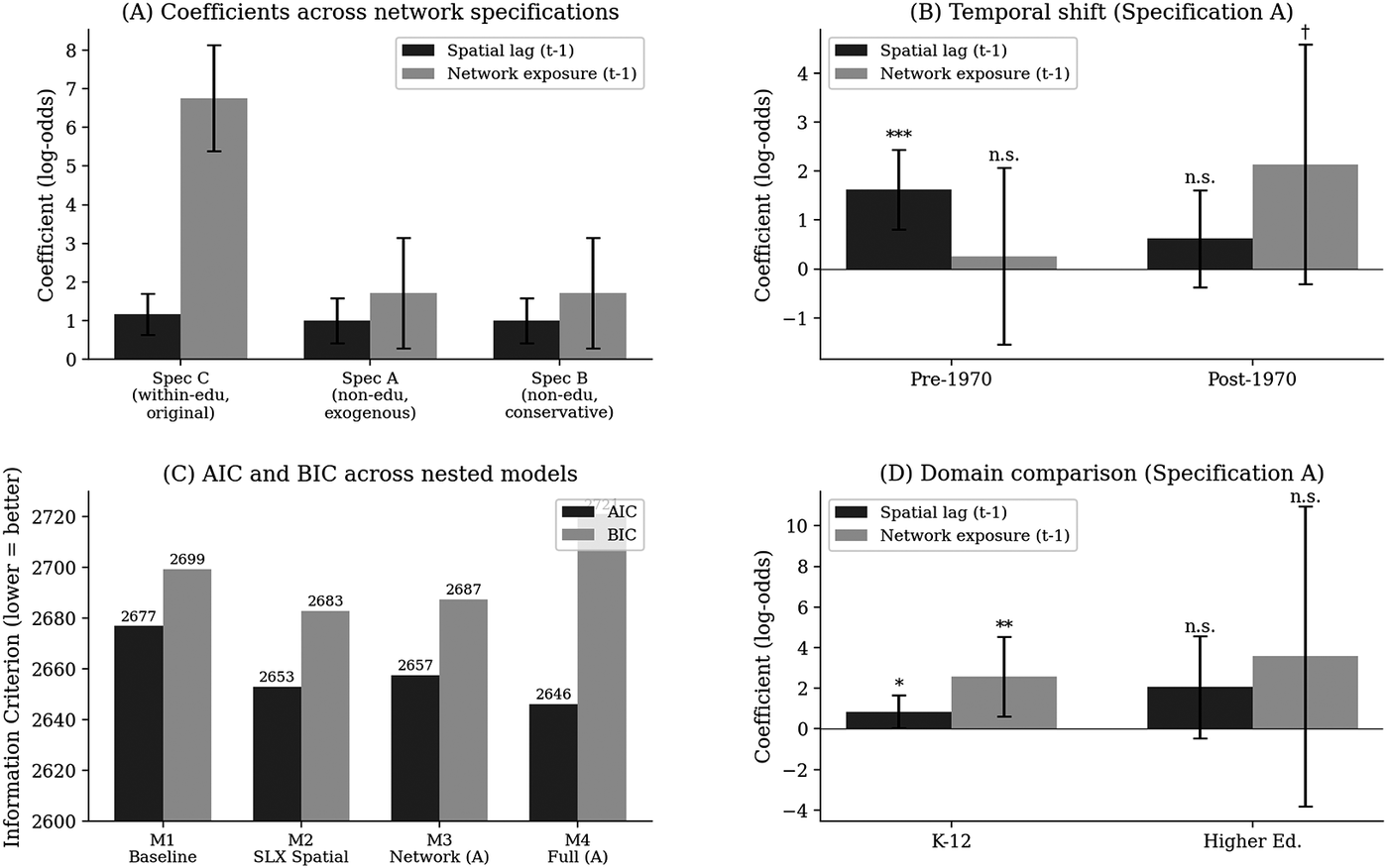
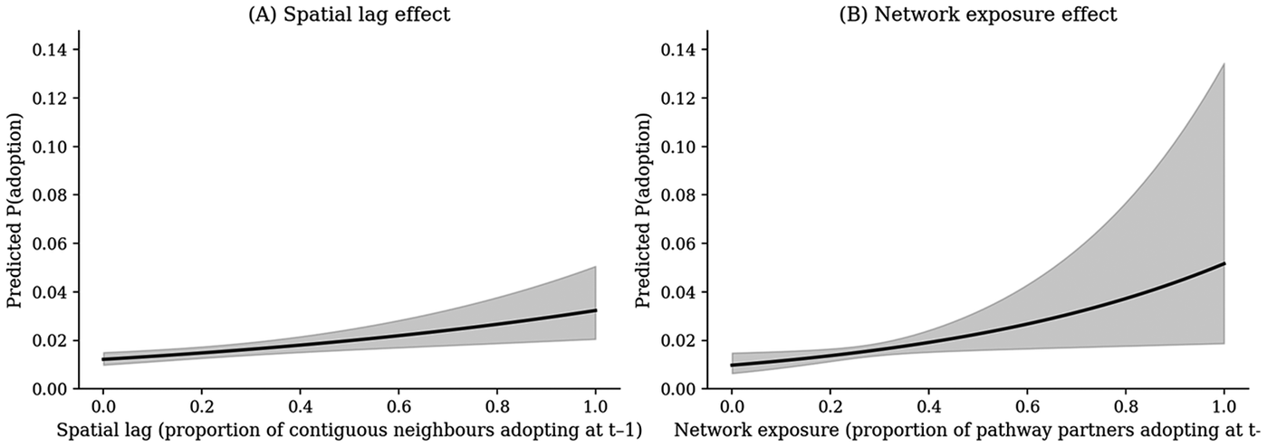
In Table 3, I report the four-model sequence using Specification A (the exogenous policy-pathway network constructed from non-education SPID policies). Figure 1 displays the principal coefficient estimates and information-criterion comparisons. Figure 2 shows the contiguity and policy-pathway networks side by side for visual comparison. Figure 3 reports predicted adoption probabilities across the observed range of the spatial lag and network exposure.
SLX discrete-time logistic survival models (Specification A, exogenous network)

Table 3. Long description
The table compares four models: M 1 baseline, M 2 S L X, M 3 network, and M 4 full.
Key variables and coefficients (standard errors in parentheses):
* Spatial lag (t minus 1): M 2 is 1.365*** (0.266); M 4 is 0.998*** (0.297).
* Network exposure (t minus 1, Spec A): M 3 is 2.755*** (0.672); M 4 is 1.710** (0.729).
* Cumulative adoption: M 1 is 2.781*** (0.247); M 2 is 1.621*** (0.343); M 3 is 0.135 (0.715); M 4 is 0.409 (0.723).
* Time since earliest adoption: All models show approximately -0.068*** or -0.069*** (0.006).
* Geographic degree centrality: M 4 is -4.733*** (1.810).
* Network degree centrality: M 4 is 0.284 (0.328).
* Region dummies: No for M 1, M 2, M 3; Yes for M 4.
* Constant: Ranges from -3.95*** to -4.31***.
Model Statistics for all models:
* N (state-policy-years): 13,112.
* Events (adoptions): 301.
* Log-likelihood: M 1 (-1,335.5), M 2 (-1,322.5), M 3 (-1,324.7), M 4 (-1,313.1).
* A I C: M 1 (2,676.9), M 2 (2,652.9), M 3 (2,657.5), M 4 (2,646.2).
* B I C: M 1 (2,699.4), M 2 (2,682.8), M 3 (2,687.4), M 4 (2,721.0).
* McFadden pseudo-R super 2: M 1 (0.068), M 2 (0.078), M 3 (0.076), M 4 (0.084).
Significance levels: * p < 0.10; ** p < 0.05; *** p < 0.01.
Note: Standard errors in parentheses. Network exposure is constructed using Specification A: Jaccard similarity on the 714 non-education policies in SPID v1.2. AIC favors the Full model (M4); BIC favors the parsimonious M2 (SLX-only); both criteria are reported for transparency. *p < 0.10; **p < 0.05; ***p < 0.01.
(a) Spatial-lag and network-exposure coefficients in the Full model under three network specifications. The within-education Jaccard (Spec C) produces network coefficients much larger than the exogenous specifications (A, B), evidence of within-domain endogeneity in Spec C. (b) Era-split coefficients showing the temporal shift from spatial-dominated to network-dominated diffusion. (c) AIC and BIC across the four nested models. (d) Domain comparison showing both channels significant in K-12 and underpowered in Higher Education. †p < 0.10, *p < 0.05, **p < 0.01, ***p < 0.001.

Figure 1. Long description
Panel A, Coefficients across network specifications, shows three groups on the x-axis. Spec C (within-edu, original) has a low spatial lag coefficient around 1 and a very high network exposure coefficient near 7. Spec A (non-edu, exogenous) and Spec B (non-edu, conservative) both show lower, similar coefficients for both variables, ranging between 1 and 2.
Panel B, Temporal shift (Specification A), compares Pre-1970 and Post-1970 eras. Pre-1970 shows a significant spatial lag (marked with three asterisks) and negligible network exposure. Post-1970 shows a decrease in spatial lag and an increase in network exposure (marked with a dagger symbol), indicating a shift in diffusion dominance.
Panel C, A I C and B I C across nested models, displays four models: M 1 Baseline, M 2 S L X Spatial, M 3 Network (A), and M 4 Full (A). The y-axis measures Information Criterion where lower is better. A I C values decrease from 2677 in M 1 to 2646 in M 4. B I C values fluctuate, with M 2 being the lowest at 2683 and M 4 at 2707.
Panel D, Domain comparison (Specification A), compares K-12 and Higher Ed. In K-12, both spatial lag (one asterisk) and network exposure (two asterisks) are significant. In Higher Ed., both coefficients are positive but marked n.s. for non-significant, with much larger error bars.
(a) Contiguity network with 107 edges and density 0.087, by definition planar with strong regional clustering. (b) Policy-pathway network (Specification A, exogenous) with 613 edges and density 0.500, exhibiting substantial cross-regional ties. (c) Kaplan–Meier survival curves by Census region. (d) Temporal clustering of adoption events 1896–2017.

Figure 2. Long description
The figure consists of four panels labeled A through D.
* Panel A: Contiguity Network. A planar network diagram where nodes represent U S states labeled with two-letter initialisms. Nodes are colored by Census region: Northeast (black), Midwest (dark gray), South (medium gray), and West (light gray). The network shows strong regional clustering with 107 edges.
* Panel B: Policy-Pathway Network. A dense network with 613 edges showing substantial cross-regional ties. Nodes are more tightly packed than in Panel A, with A K and H I appearing as isolated nodes on the right and bottom.
* Panel C: Regional Survival Curves. A Kaplan-Meier plot with the Y-axis representing Survival Probability from 0.0 to 1.0 and the X-axis representing Years since first adoption from 0 to 120. Four lines represent the regions. The Northeast (solid black line) shows the fastest decline in survival probability, while the West (dotted line) and South (dash-dot line) maintain higher survival probabilities over time.
* Panel D: Temporal Clustering of Adoptions. A histogram with a superimposed trend line. The Y-axis is the Number of adoption events (0 to 20) and the X-axis is the Year (1900 to 2020). Significant spikes in adoption events occur around 1970 and 2010, with smaller clusters in the 1930s and 1960s.
Predicted adoption probability across the observed range of the spatial lag and network exposure under the Full model with Specification A, holding other covariates at sample means. Network exposure shifts predicted probability from approximately 0.010 to 0.052; the spatial lag shifts predicted probability from approximately 0.012 to 0.032. The 95% confidence interval is shaded; the wider band at the upper end of the network-exposure scale reflects the smaller number of high-network-exposure observations in the panel.

Figure 3. Long description
The figure consists of two side-by-side line graphs.
Panel A, titled Spatial lag effect. The vertical Y axis is labeled Predicted P adoption and ranges from 0.00 to 0.14 in increments of 0.02. The horizontal X axis is labeled Spatial lag (proportion of contiguous neighbours adopting at t minus 1) and ranges from 0.0 to 1.0. A solid black line starts at approximately 0.012 on the Y axis and follows a gentle upward curve to reach approximately 0.032 at the far right. A light gray shaded band representing the 95 percent confidence interval surrounds the line, widening slightly as it moves from left to right.
Panel B, titled Network exposure effect. The Y axis is identical to Panel A. The horizontal X axis is labeled Network exposure (proportion of pathway partners adopting at t minus 1) and ranges from 0.0 to 1.0. A solid black line starts at approximately 0.010 and follows a steeper upward curve than in Panel A, reaching approximately 0.052 at the far right. The gray shaded confidence interval is narrow at the start but expands significantly at the upper end of the scale, forming a wide wedge shape reaching from 0.02 to over 0.13 on the Y axis.
The baseline model achieves AIC = 2,677 and pseudo-R 2 = 0.068. Adding the temporally lagged spatial lag improves the fit substantially (AIC = 2,653); the spatial-lag coefficient is 1.37 (SE = 0.27, p < 0.001), supporting Hypothesis 1. Substituting network exposure (Specification A) yields a network-exposure coefficient of 2.76 (SE = 0.67, p < 0.001), supporting Hypothesis 2. The Full model retains both, with the spatial-lag coefficient at 1.00 (SE = 0.30, p < 0.001) and the network-exposure coefficient at 1.71 (SE = 0.73, p = 0.019). The Full model achieves the lowest AIC (2,646) but a higher BIC (2,721) than the parsimonious M2 (SLX-only) model (BIC = 2,683). The preference of BIC for the parsimonious model reflects the additional centrality and region covariates carrying penalty weight without proportional fit gains; both criteria are reported for transparency. The substantive finding of two independent channels is robust under both criteria.
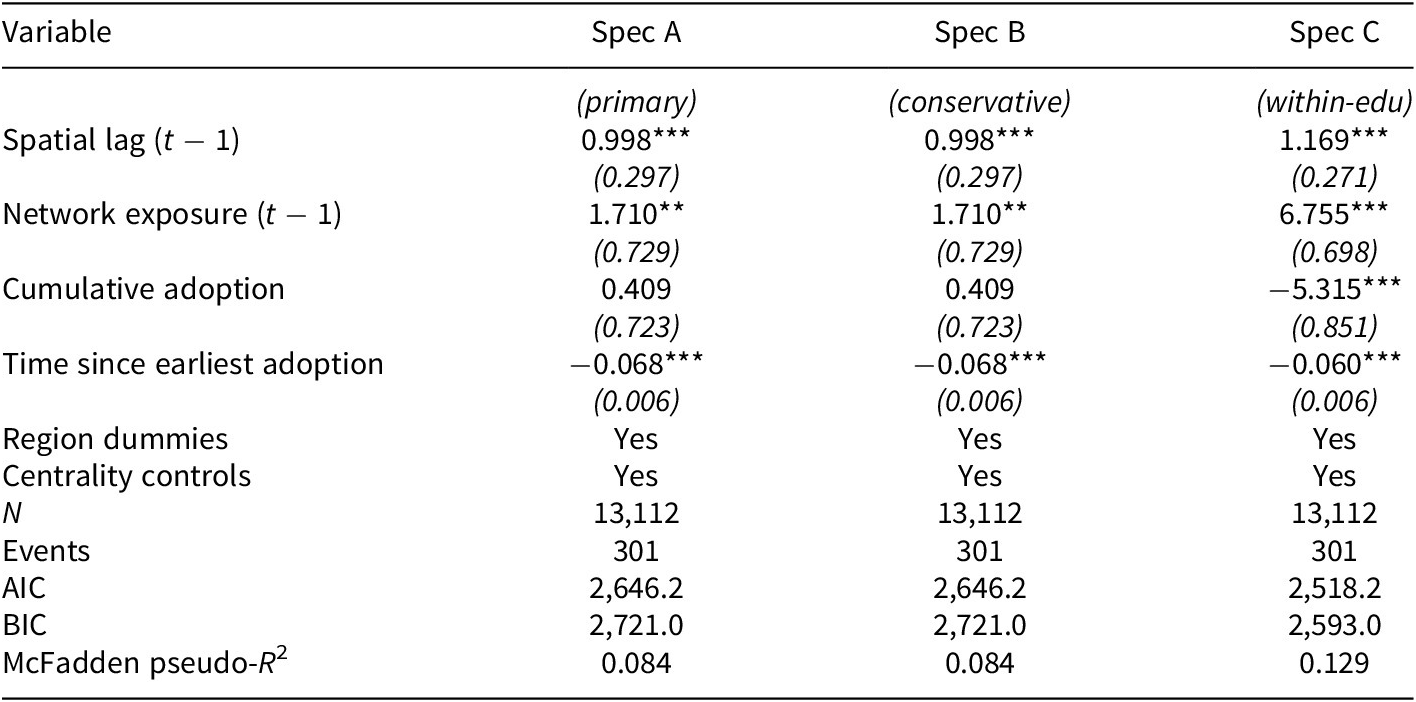
The contrast with Specification C (the within-education Jaccard) is informative. Under Specification C, the network-exposure coefficient is 6.76 (SE = 0.70), nearly four times larger than under the exogenous Specification A. The contrast indicates that the within-domain network partially re-encodes the dependent variable. Table 4 compares the Full model under all three network specifications. The exogenous estimate is therefore treated as primary.
Full model under three network specifications

Table 4. Long description
The table consists of four columns: Variable, Spec A (primary), Spec B (conservative), and Spec C (within-edu).
* Spatial lag (t minus 1): Spec A and B both show 0.998 with significance p < 0.01 and standard error 0.297. Spec C shows 1.169 with significance p < 0.01 and standard error 0.271.
* Network exposure (t minus 1): Spec A and B both show 1.710 with significance p < 0.05 and standard error 0.729. Spec C shows 6.755 with significance p < 0.01 and standard error 0.698.
* Cumulative adoption: Spec A and B both show 0.409 with standard error 0.723. Spec C shows minus 5.315 with significance p < 0.01 and standard error 0.851.
* Time since earliest adoption: Spec A and B both show minus 0.068 with significance p < 0.01 and standard error 0.006. Spec C shows minus 0.060 with significance p < 0.01 and standard error 0.006.
* Region dummies and Centrality controls: All three specifications are marked Yes.
* Model Statistics: N is 13,112 and Events are 301 for all. A I C is 2,646.2 for Spec A and B, and 2,518.2 for Spec C. B I C is 2,721.0 for Spec A and B, and 2,593.0 for Spec C. McFadden pseudo-R super 2 is 0.084 for Spec A and B, and 0.129 for Spec C.
Note: Approximately 75% of the network coefficient under Specification C (6.76) is attributable to within-domain endogeneity; the exogenous coefficient under Specifications A and B (1.71) is statistically significant but substantively smaller. The spatial-lag coefficient is stable across specifications. *p < 0.10; **p < 0.05; ***p < 0.01.
Policy-level random effects
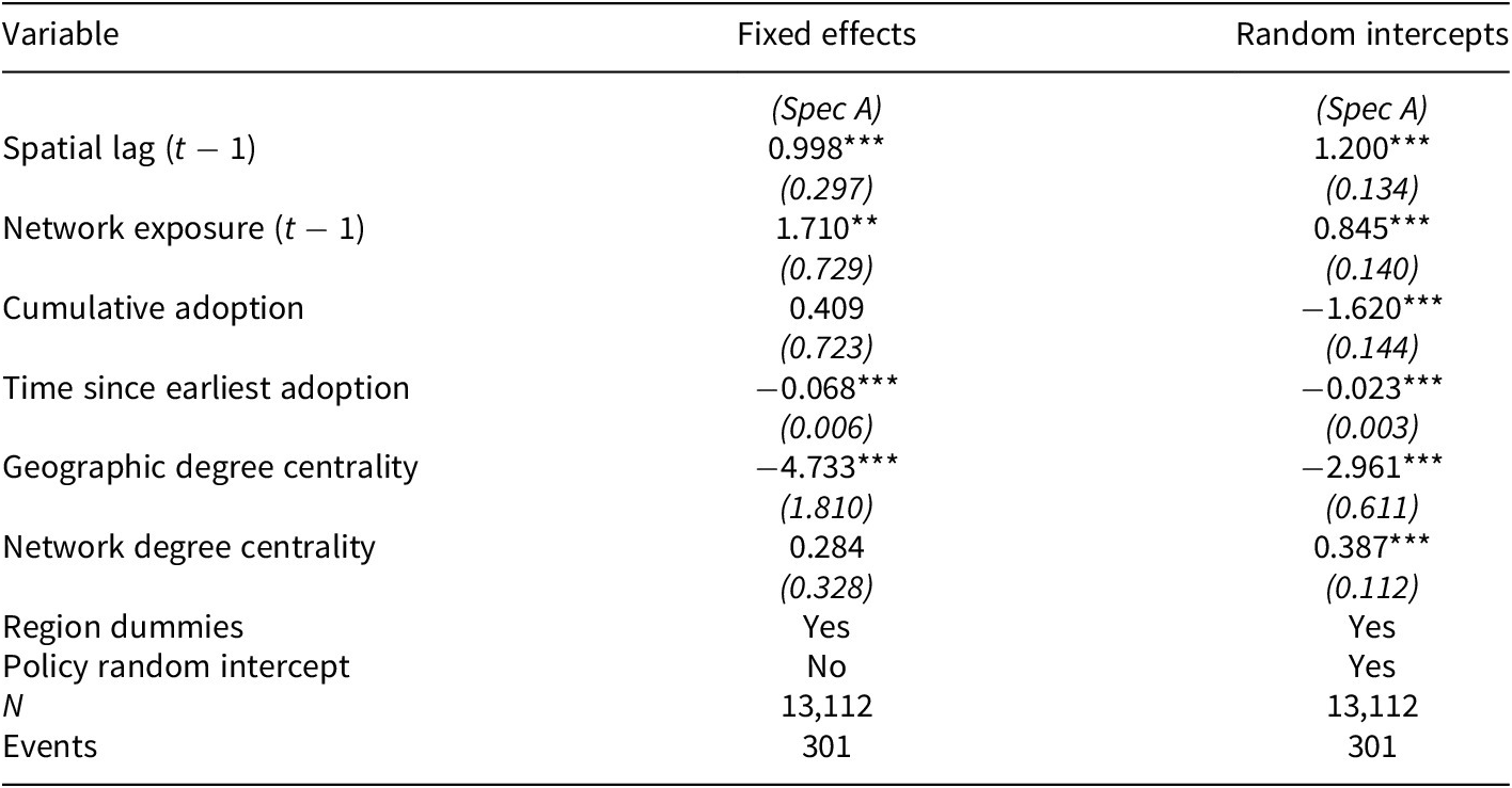
To address the concern that policies have very different baseline adoption rates, the Full model is re-estimated as a Bayesian binomial mixed-GLM with policy-level random intercepts (Table 5). Under this specification, the spatial-lag coefficient is 1.20 (SE = 0.13, p < 0.001), slightly larger than the fixed-effects estimate, while the network-exposure coefficient is 0.85 (SE = 0.14, p < 0.001), substantially smaller than the fixed-effects estimate of 1.71. A portion of what the fixed-effects model attributes to the network channel is absorbed by policy-level baseline-rate heterogeneity in the random-effects specification. The substantive conclusion that both channels are independently and statistically significantly associated with adoption hazard survives this more conservative specification, although the magnitude of the network channel is smaller than the fixed-effects model suggests. The network coefficient shrinks across a sequence of progressively more demanding specifications, from 6.76 (within-domain endogenous) to 1.71 (fixed-effects with exogenous network) to 0.85 (random-intercept with exogenous network); the random-intercept estimate is reported as the most conservative defensible figure.
Full model with policy-level random intercepts (Bayesian binomial mixed-GLM)

Table 5. Long description
The table contains three columns: Variable, Fixed effects (Spec A), and Random intercepts (Spec A).
* Spatial lag (t minus 1): Fixed effects 0.998 (0.297); Random intercepts 1.200 (0.134). Both are significant at p < 0.01.
* Network exposure (t minus 1): Fixed effects 1.710 (0.729) significant at p < 0.05; Random intercepts 0.845 (0.140) significant at p < 0.01.
* Cumulative adoption: Fixed effects 0.409 (0.723); Random intercepts minus 1.620 (0.144) significant at p < 0.01.
* Time since earliest adoption: Fixed effects minus 0.068 (0.006); Random intercepts minus 0.023 (0.003). Both are significant at p < 0.01.
* Geographic degree centrality: Fixed effects minus 4.733 (1.810); Random intercepts minus 2.961 (0.611). Both are significant at p < 0.01.
* Network degree centrality: Fixed effects 0.284 (0.328); Random intercepts 0.387 (0.112) significant at p < 0.01.
* Region dummies: Yes for both models.
* Policy random intercept: No for Fixed effects; Yes for Random intercepts.
* N: 13,112 for both models.
* Events: 301 for both models.
Standard errors are provided in parentheses below each coefficient. Significance levels are indicated by asterisks: one for p < 0.10, two for p < 0.05, and three for p < 0.01.
Note: Standard errors in parentheses. The right column uses the Bayesian binomial mixed-GLM (statsmodels BinomialBayesMixedGLM, variational Bayes) with policy-level random intercepts. Both spatial and network channels remain significantly associated with adoption hazard under the more conservative random-effects specification, although the network coefficient shrinks from 1.71 to 0.85, indicating that some apparent network effect under fixed effects is absorbed by policy-level baseline-rate heterogeneity. The spatial-lag coefficient is stable. *p < 0.10; **p < 0.05; ***p < 0.01.
Temporal shift: pre-1970 versus post-1970
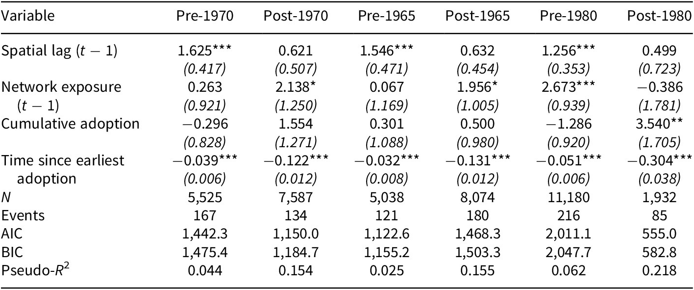
Separate models estimated for policies originating before 1970 (four policies, 167 events, 5,525 observations) and after 1970 (six policies, 134 events, 7,587 observations) reveal a pronounced shift, supporting Hypothesis 3. For pre-1970 policies, only the spatial channel is statistically detectable (b = 1.63, p < 0.001); the network coefficient is statistically zero (b = 0.26, p = 0.78). For post-1970 policies, the spatial channel attenuates to non-significance (b = 0.62, p = 0.22) and the network channel emerges as marginally significant (b = 2.14, p = 0.087). Table 6 reports the era-split estimates with sensitivity at 1965 and 1980 cut-points; the pattern is robust at 1965 and 1970.
Time-varying mechanism analysis (Specification A)

Table 6. Long description
The table compares coefficients across six columns: Pre-1970, Post-1970, Pre-1965, Post-1965, Pre-1980, and Post-1980.
Key variables and their coefficients (standard errors in parentheses):
* Spatial lag (t minus 1): Shows significant positive effects in all ‘Pre’ periods (1.625, 1.546, and 1.256, all p < 0.01) but loses significance in all ‘Post’ periods.
* Network exposure (t minus 1): Shows significant positive effects in Post-1970 (2.138, p < 0.10), Post-1965 (1.956, p < 0.10), and Pre-1980 (2.673, p < 0.01).
* Cumulative adoption: Significant only in Post-1980 (3.540, p < 0.05).
* Time since earliest adoption: Consistently negative and highly significant (p < 0.01) across all six models, ranging from -0.032 to -0.304.
Model Statistics:
* N (Sample size): Ranges from 1,932 (Post-1980) to 11,180 (Pre-1980).
* Events: Ranges from 85 to 216.
* A I C: Ranges from 555.0 to 2,011.1.
* B I C: Ranges from 582.8 to 2,047.7.
* Pseudo-R super 2: Increases in later periods, peaking at 0.218 in Post-1980.
Note: The pattern of stronger spatial and weaker network channels in the earlier era, reversing in the later era, is robust at the 1965 and 1970 cut-points. The 1980 cut-point is dominated by the Military Children Compact. *p < 0.10; **p < 0.05; ***p < 0.01.
This pattern is consistent with the institutional-layering interpretation: the pre-1970 era was, in detectable signal, a purely geographic regime in which states attended to what their neighbors did and the policy-pathway network exerted no measurable independent pull; the post-1970 era is a network-mediated regime.
Domain comparison: K-12 versus higher education
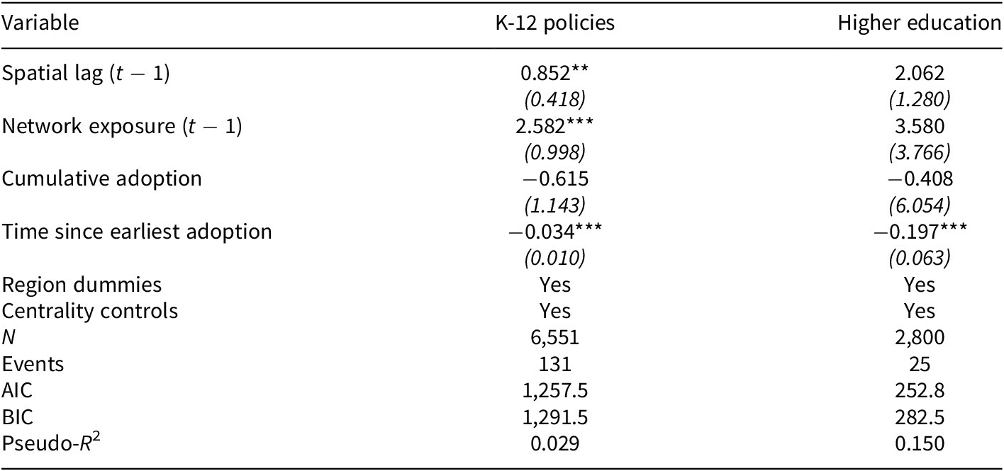
Separate models for K-12 policies (four policies, 131 events) and higher-education policies (two policies, 25 events) reveal domain-specific dynamics (Table 7). For K-12 policies, both the spatial channel (b = 0.85, p = 0.041) and the network channel (b = 2.58, p = 0.010) are statistically significant. For higher-education policies, the picture is genuinely uncertain. The spatial coefficient (b = 2.06, p = 0.107) and network coefficient (b = 3.58, p = 0.342) are each positive in sign, but neither reaches conventional significance, and the 95% confidence intervals are wide. The K-12 finding supports Hypothesis 4 in the predicted direction; the higher-education side of the Hypothesis 4 contrast rests on theoretical motivation rather than on decisive empirical evidence given the limited number of higher-education events.
Domain comparison: K-12 versus higher education (Specification A)

Table 7. Long description
A table with three columns: Variable, K-12 policies, and Higher education.
* Spatial lag (t minus 1): K-12 is 0.852 with two asterisks (standard error 0.418); Higher education is 2.062 (standard error 1.280).
* Network exposure (t minus 1): K-12 is 2.582 with three asterisks (standard error 0.998); Higher education is 3.580 (standard error 3.766).
* Cumulative adoption: K-12 is minus 0.615 (standard error 1.143); Higher education is minus 0.408 (standard error 6.054).
* Time since earliest adoption: K-12 is minus 0.034 with three asterisks (standard error 0.010); Higher education is minus 0.197 with three asterisks (standard error 0.063).
* Region dummies: Yes for both.
* Centrality controls: Yes for both.
* N: K-12 is 6,551; Higher education is 2,800.
* Events: K-12 is 131; Higher education is 25.
* A I C: K-12 is 1,257.5; Higher education is 252.8.
* B I C: K-12 is 1,291.5; Higher education is 282.5.
* Pseudo-R super 2: K-12 is 0.029; Higher education is 0.150.
Note: Two asterisks indicate p < 0.05 and three asterisks indicate p < 0.01.
Note: K-12 policies (n = 4): Corporal Punishment Ban, Elementary Teacher Cert., HS Teacher Cert., School Choice. Higher Education policies (n = 2): In-State Tuition (Undocumented), Student Borrowing Capacity Act. The higher-education subsample contains only 25 events and is statistically underpowered; both coefficients are positive in sign but neither reaches significance. The K-12 finding supports Hypothesis 4. *p < 0.10; **p < 0.05; ***p < 0.01.
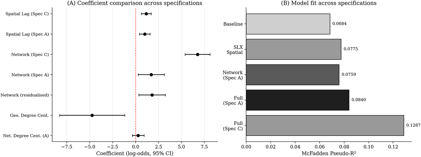
Figure 4 summarizes the cross-specification comparison: panel A is a forest plot of coefficient estimates across Specifications A and C alongside the residualized network-exposure estimate, and panel B compares pseudo-R 2 values, making the consequences of within-domain versus exogenous network construction visually explicit.
(a) Forest plot comparing coefficient estimates across all primary specifications. The spatial-lag estimate is stable across Specifications A and C; the network-exposure estimate is much larger under Specification C (within-education) than under the exogenous Specification A. The residualized network-exposure estimate confirms that the network channel operates substantially independently of geography. (b) Pseudo-R 2 comparison; the apparent fit advantage of Specification C reflects partial re-encoding of the dependent variable through within-domain network construction.

Figure 4. Long description
Panel A is a forest plot titled Coefficient comparison across specifications. The x-axis represents Coefficient log-odds with a 95 percent C I, ranging from negative 7.5 to 7.5. A vertical dashed red line marks the zero point. From top to bottom, the estimates are:
* Spatial Lag (Spec C): Positive, approximately 1.2.
* Spatial Lag (Spec A): Positive, approximately 1.0.
* Network (Spec C): Large positive, approximately 6.8.
* Network (Spec A): Positive, approximately 1.8.
* Network (residualised): Positive, approximately 1.8.
* Geo. Degree Cent.: Large negative, approximately negative 4.8.
* Net. Degree Cent. (A): Near zero, slightly positive.
Panel B is a horizontal bar chart titled Model fit across specifications. The x-axis measures McFadden Pseudo-R super 2 from 0.00 to 0.12. From top to bottom, the bars and their values are:
* Baseline: Light gray, 0.0684.
* S L X Spatial: Medium gray, 0.0775.
* Network (Spec A): Dark gray, 0.0759.
* Full (Spec A): Black, 0.0840.
* Full (Spec C): Medium gray, 0.1287.
Robustness: residualized network exposure. To address the concern that the spatial lag and network exposure may capture overlapping channels, the model was re-estimated with network exposure residualized on the spatial lag. The residualized network-exposure coefficient is 1.79 (SE = 0.74, p = 0.015), confirming that the network channel operates substantially independently of geography. The dyadic correlation between the contiguity adjacency matrix and the Specification A network adjacency matrix is 0.23.
Spatial Durbin model: scope conditions for SAR and SLX specifications
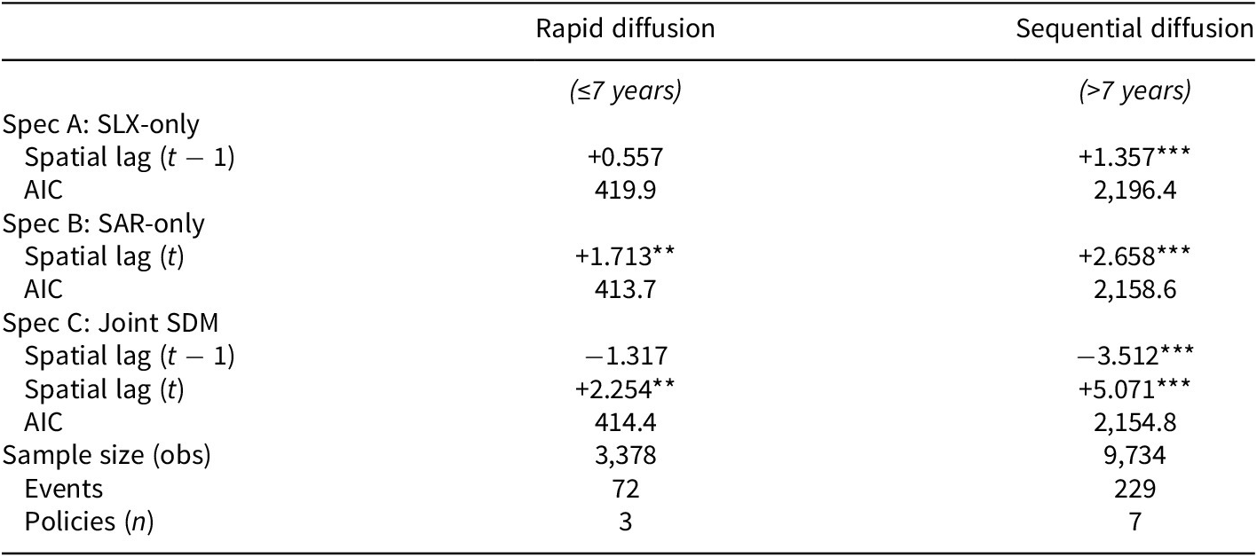
The substantive question of when SAR (contemporaneous determination) is theoretically appropriate alongside SLX (lagged determination) deserves direct empirical treatment. To address this, the 10 education policies are partitioned into a rapid-diffusion subset (those diffusing in seven years or fewer: Military Children Compact, Student Borrowing Capacity Act, School Choice; n = 3 policies, 72 events, 3,378 observations) and a sequential-diffusion subset (the remaining seven policies, 229 events, 9,734 observations). On each subset, the SLX-only specification, the SAR-only specification, and the joint SDM are estimated. Table 8 reports the results.
Spatial Durbin model by diffusion speed: empirical resolution of SLX versus SAR

Table 8. Long description
The table is organized into three columns: the first for variables and specifications, the second for Rapid diffusion (less than or equal to 7 years), and the third for Sequential diffusion (greater than 7 years).
* Spec A: S L X-only
- Spatial lag (t minus 1): +0.557 for Rapid; +1.357 with three asterisks for Sequential.
- A I C: 419.9 for Rapid; 2,196.4 for Sequential.
* Spec B: S A R-only
- Spatial lag (t): +1.713 with two asterisks for Rapid; +2.658 with three asterisks for Sequential.
- A I C: 413.7 for Rapid; 2,158.6 for Sequential.
* Spec C: Joint S D M
- Spatial lag (t minus 1): -1.317 for Rapid; -3.512 with three asterisks for Sequential.
- Spatial lag (t): +2.254 with two asterisks for Rapid; +5.071 with three asterisks for Sequential.
- A I C: 414.4 for Rapid; 2,154.8 for Sequential.
* Summary Statistics
- Sample size (obs): 3,378 for Rapid; 9,734 for Sequential.
- Events: 72 for Rapid; 229 for Sequential.
- Policies (n): 3 for Rapid; 7 for Sequential.
Note: Asterisks indicate p-values where one asterisk is p less than 0.10, two asterisks is p less than 0.05, and three asterisks is p less than 0.01.
Note: For rapid-diffusion policies, the SAR-only specification recovers a statistically significant contemporaneous spatial signal (b = 1.71, p = 0.010) that the SLX-only specification misses entirely. For sequential-diffusion policies, both specifications detect signal; the joint SDM exhibits multicollinearity because the contemporaneous (year − t) variable mechanically includes lagged (year t − 1) information. The SAR-vs-SLX choice should be governed by the temporal structure of the diffusion process. Rapid policies: Military Children Compact (six years), Student Borrowing (three years), School Choice (five years). Sequential policies: the remaining 7 of 10 policies. *p < 0.10; **p < 0.05; ***p < 0.01.
The pattern in Figure 5 directly addresses the SAR-versus-SLX question. For rapid-diffusion policies, contemporaneous neighbor adoption is the data-generating process the SAR specification correctly captures; the SLX-only specification fails to detect the signal because it excludes same-year information. For sequential-diffusion policies, both specifications detect signal, but the joint SDM exhibits the strong multicollinearity expected when the contemporaneous variable mechanically subsumes the lagged information; in this case the substantive theory of sequential observation favors SLX as the appropriate primary specification. The practical implication for diffusion methodology is that the SAR-versus-SLX choice should be driven by the substantive theory of the diffusion process rather than by a default ranking.
SLX-only, SAR-only, and joint SDM coefficient estimates on rapid-diffusion (panel A, 3 policies, 72 events) and sequential-diffusion (panel B, 7 policies, 229 events) subsamples. For rapid-diffusion policies, SAR-only recovers a significant spatial signal (b = 1.71, p = 0.010) while SLX-only does not (b = 0.56, p = 0.55); the joint SDM allocates the signal to the contemporaneous term. For sequential-diffusion policies, both SLX-only (b = 1.36, p < 0.001) and SAR-only (b = 2.66, p < 0.001) recover significant signals; the joint SDM exhibits the multicollinearity expected when the contemporaneous variable is a strict superset of the lagged variable. The substantive interpretation is that the SAR–SLX choice should be governed by the temporal structure of the diffusion process under study.

Figure 5. Long description
A two-panel horizontal forest plot. The x-axis represents the Coefficient in log-odds with 95 percent C I. A vertical dashed red line marks the zero baseline.
Panel A, titled Rapid-diffusion policies (n equals 3 policies, 7 years or less), shows four estimates:
* S L X-only (b on slag t minus 1): Point estimate near 0.5 with a wide error bar crossing zero, labeled n.s.
* S A R-only (b on slag t): Point estimate near 1.7 with error bars entirely above zero, labeled with two asterisks.
* Joint S D M (b on slag t minus 1): Point estimate near minus 1.3 with a very wide error bar crossing zero, labeled n.s.
* Joint S D M (b on slag t): Point estimate near 2.3 with error bars entirely above zero, labeled with two asterisks.
Panel B, titled Sequential-diffusion policies (n equals 7 policies, greater than 7 years), shows four estimates:
* S L X-only (b on slag t minus 1): Point estimate near 1.4 with error bars above zero, labeled with three asterisks.
* S A R-only (b on slag t): Point estimate near 2.7 with error bars above zero, labeled with three asterisks.
* Joint S D M (b on slag t minus 1): Point estimate near minus 3.5 with error bars entirely below zero, labeled with three asterisks.
* Joint S D M (b on slag t): Point estimate near 5.1 with error bars entirely above zero, labeled with three asterisks.
Post-1960 robustness with state-innovation control
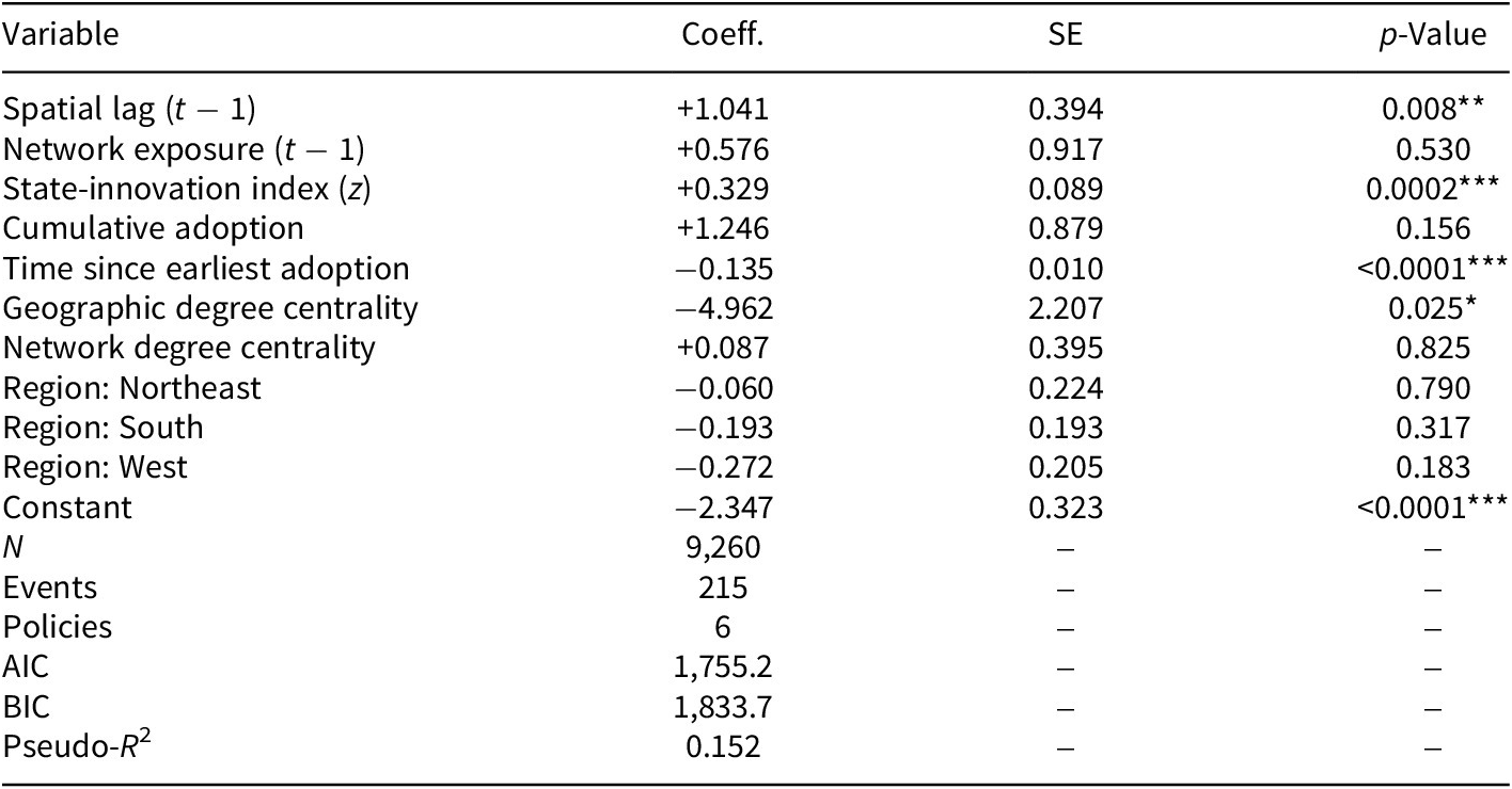
Regional dummies are a coarse proxy for state-level heterogeneity. While extending the Berry et al. ideology scores or Squire index back to 1896 is not possible, a state-innovation activity index is constructed from the cumulative count of non-education SPID policy adoptions per state-year, standardized. This proxy captures the underlying construct, the differential propensity of states to adopt new policies, that the standard ideology and professionalism controls would also measure. On the post-1960 subsample (9,260 observations, 215 events, six policies), the Full model with this control yields a spatial-lag coefficient of 1.04 (SE = 0.39, p = 0.008), a state-innovation index coefficient of 0.33 (SE = 0.09, p = 0.0002, highly significant), and a network-exposure coefficient that is no longer statistically significant (b = 0.58, SE = 0.92, p = 0.53). Table 9 reports the full estimates. In the post-1960 sample, much of what the fixed-effects model attributes to the network channel may reflect general state policy-activity propensity captured by the innovation index. The spatial channel remains robust. The implications are discussed in the “Robustness of the network channel” section.
Post-1960 robustness with state-innovation activity control

Table 9. Long description
The table consists of four columns: Variable, Coeff. (Coefficient), S E (Standard Error), and p-Value.
* Spatial lag (t minus 1): Coeff. +1.041, S E 0.394, p-Value 0.008 (significant at p < 0.01).
* Network exposure (t minus 1): Coeff. +0.576, S E 0.917, p-Value 0.530.
* State-innovation index (z): Coeff. +0.329, S E 0.089, p-Value 0.0002 (significant at p < 0.001).
* Cumulative adoption: Coeff. +1.246, S E 0.879, p-Value 0.156.
* Time since earliest adoption: Coeff. -0.135, S E 0.010, p-Value < 0.0001 (significant at p < 0.001).
* Geographic degree centrality: Coeff. -4.962, S E 2.207, p-Value 0.025 (significant at p < 0.05).
* Network degree centrality: Coeff. +0.087, S E 0.395, p-Value 0.825.
* Region Northeast: Coeff. -0.060, S E 0.224, p-Value 0.790.
* Region South: Coeff. -0.193, S E 0.193, p-Value 0.317.
* Region West: Coeff. -0.272, S E 0.205, p-Value 0.183.
* Constant: Coeff. -2.347, S E 0.323, p-Value < 0.0001 (significant at p < 0.001).
Model statistics at the bottom include:
* N: 9,260.
* Events: 215.
* Policies: 6.
* A I C: 1,755.2.
* B I C: 1,833.7.
* Pseudo-R super 2: 0.152.
Note: Post-1960 subsample (six policies entering their diffusion window in 1960 or later). The state-innovation index is the standardized cumulative count of non-education SPID policy adoptions per state-year, available across 1896–2017. The state-innovation control is highly significant; the spatial-lag coefficient remains robust; the network-exposure coefficient drops to non-significance, suggesting that in the post-1960 sample much of the apparent network effect is absorbed by general state policy-activity propensity. The temporal-shift finding (Hypothesis 3) does not depend on this specification. *p < 0.05; **p < 0.01; ***p < 0.001.
SPID-wide methodological replication
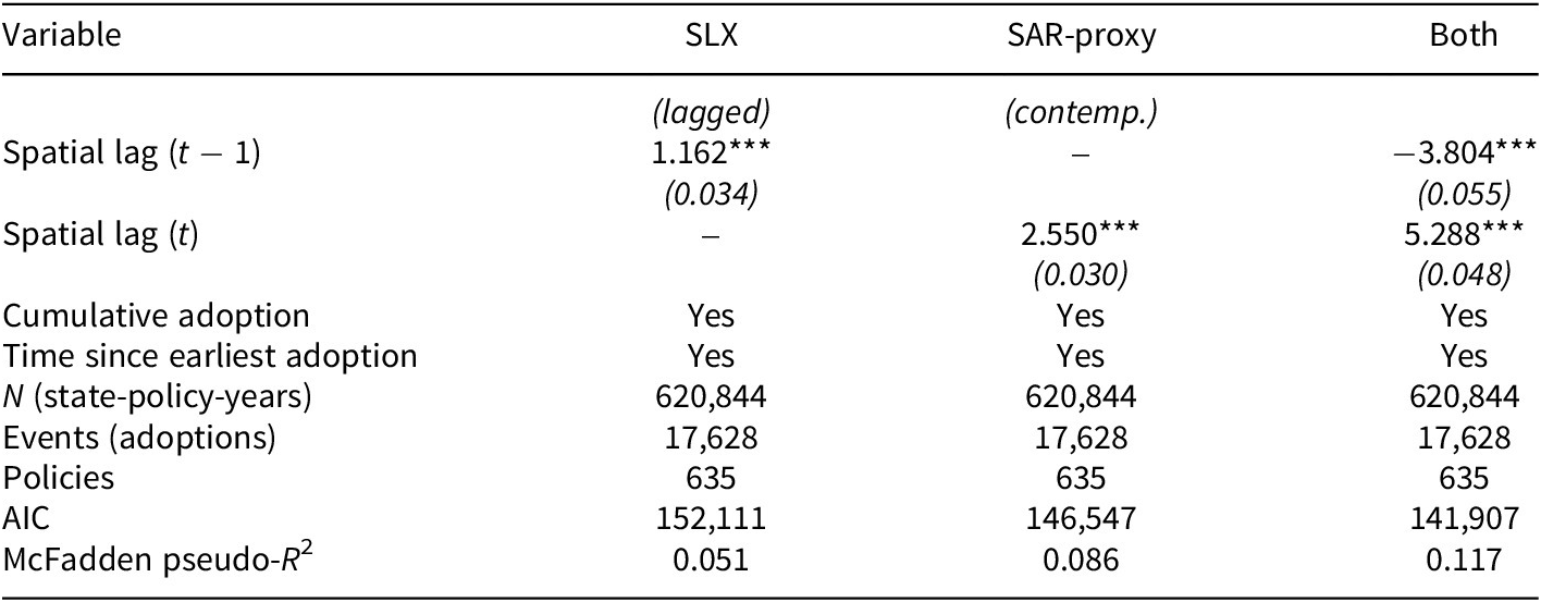
The SPID-wide replication on 635 policies and 17,628 adoption events (Table 10) finds that both temporally lagged spatial influence (θ = +1.16, p < 0.001) and contemporaneous spatial influence (ρ-proxy = +2.55, p < 0.001) are highly significant. The SDM analysis reported in “Spatial Durbin model: scope conditions for SAR and SLX specifications” section clarifies why: the SAR specification detects spatial determination for rapid-diffusion policies that SLX misses, while SLX detects sequential influence that SAR conflates with mechanically included contemporaneous neighbor activity. The choice between SAR and SLX is therefore a substantive specification decision driven by the temporal structure of the diffusion process, not a universal methodological ranking. For sequential-observation diffusion processes, which describe the bulk of the 10 education policies analyzed in this study, SLX is the appropriate primary specification. For rapid-bandwagon, conformity-driven, or crisis-clustered diffusion processes, SAR remains theoretically warranted.
SPID-wide replication of SAR versus SLX specifications

Table 10. Long description
The table consists of four columns: Variable, S L X (lagged), S A R-proxy (contemporaneous), and Both.
* Spatial lag (t minus 1): S L X is 1.162 with a standard error of 0.034; S A R-proxy is null; Both is negative 3.804 with a standard error of 0.055.
* Spatial lag (t): S L X is null; S A R-proxy is 2.550 with a standard error of 0.030; Both is 5.288 with a standard error of 0.048.
* Cumulative adoption: Yes for all three models.
* Time since earliest adoption: Yes for all three models.
* N (state-policy-years): 620,844 for all three models.
* Events (adoptions): 17,628 for all three models.
* Policies: 635 for all three models.
* A I C: S L X is 152,111; S A R-proxy is 146,547; Both is 141,907.
* McFadden pseudo-R super 2: S L X is 0.051; S A R-proxy is 0.086; Both is 0.117.
All spatial lag coefficients are significant at the p < 0.001 level, indicated by three asterisks.
Note: Replication on the full SPID v1.2 universe of policies with at least five adoptions (635 of 724 policies, 17,628 of 17,823 adoptions). Both lagged and contemporaneous spatial signals are highly significant. SAR and SLX capture genuinely different aspects of spatial dependence; the choice between them is a substantive specification decision driven by the temporal structure of the diffusion process. ***p < 0.001.
Discussion
Methodological implications: SAR, SLX, and specification choice
The implication for diffusion methodology extends beyond the present analysis. Wimpy, Whitten, and Williams (Reference Wimpy, Whitten and Williams2021) argue persuasively for SLX as the default specification on the grounds that SLX coefficients have direct interpretation as marginal effects of neighbor adoption, while SAR coefficients require post-estimation derivation of marginal effects through the spatial multiplier. The empirical finding reported in “Spatial Durbin model: scope conditions for SAR and SLX specifications” section, that contemporaneous SAR can recover spatial signal that SLX misses for rapid-diffusion processes, qualifies the case for SLX as universal default. The qualification is consistent with the theoretical position taken by Cook, An, and Favero (Reference Cook, An and Favero2019), who emphasize that the choice of spatial specification should reflect the substantive theory of how spatial dependence operates in the data-generating process under study. Drolc, Gandrud, and Williams (Reference Drolc, Gandrud and Williams2021) reach a similar conclusion in their analysis of time-and-space modelling, arguing that the appropriate specification depends on the temporal structure of the dependence relationship being modelled. The empirical evidence reported in the “Spatial Durbin model: scope conditions for SAR and SLX specifications” section and “SPID-wide methodological replication” section, derived from direct estimation on subsamples partitioned by diffusion speed and on the full SPID universe of 635 policies, provides additional support for the temporal-structure-dependent specification choice these authors advocate.
Geography gives way to networks
The temporal shift from geography-mediated to network-mediated diffusion is robust across all three network specifications and all three era cut-points. The pre-1970 period is, in detectable signal, a purely geographic regime: states attended to what their neighbors did, and the policy-pathway network exerted no measurable independent pull on adoption hazard. The post-1970 period exhibits an emerging network channel and an attenuating geographic channel, with the relative importance of the two channels reversing across the consolidation window.
The substantive interpretation of this shift rests on the institutional consolidation of nationally organized interstate policy bodies between 1965 and 1975. The Education Commission of the States, founded in 1965 with bipartisan governor support, established a permanent infrastructure for interstate education policy coordination that had not previously existed. The reorganized National Conference of State Legislatures, formed in 1975 from the merger of three predecessor organizations, created a comparable infrastructure for legislative policy coordination across all policy domains. The expanded policy programs of the National Governors Association during the 1970s, and the consolidation of the Council of Chief State School Officers as a coordinating body for state education agencies, complete the picture of a structural change in how interstate policy communication is organized. Before this consolidation, policy ideas travelled primarily through the bilateral channels that geographic proximity facilitates; after the consolidation, policy ideas can travel through national professional networks that connect states regardless of physical proximity.
The temporal shift documented in the era-split models is consistent with the broader argument advanced by Mallinson (Reference Mallinson2021b) about the declining importance of geographic proximity in policy diffusion as the institutional infrastructure for interstate communication has expanded. Mallinson finds that ideological alignment increasingly conditions which states serve as reference points for policy learning, partially displacing the role of geographic proximity. The present analysis cannot directly assess ideological alignment as a channel because the available ideology measures do not extend back to the early-twentieth-century policies that anchor the pre-1970 era analysis, but the temporal pattern documented in the era-split models is consistent with the broader pattern Mallinson documents. Future work using post-1960 diffusion data could integrate the network-exposure measure developed in this study with ideological-alignment measures to disentangle the relative contributions of network position and ideological proximity in the contemporary diffusion environment.
Domain architecture and the limits of power
The K-12 finding supports the governance-architecture prediction. K-12 education in the United States is governed primarily through state agencies whose interstate cooperation runs through explicitly geographic regional compact infrastructure, including the Western Interstate Commission for Higher Education, the Southern Regional Education Board, the Midwestern Higher Education Compact, and the New England Board of Higher Education. The compact structure organizes information flow, joint programming, and shared resources around regional rather than national groupings, generating ongoing geographic clustering of K-12 policy adoption. The K-12 finding reported in Table 7 is consistent with this institutional architecture: both channels are detectable, and the spatial channel persists into the modern era to a greater extent than the all-policy aggregate model would suggest.
The higher-education finding is genuinely uncertain given the limited sample. With only 25 adoption events across two policies, neither the spatial nor the network coefficient reaches significance, and the 95% confidence intervals are wide. Both coefficients are positive in sign, consistent with the prediction that some channel of inter-state influence operates in higher-education policy diffusion, but the available data cannot adjudicate between the spatial and network channels in this domain. The theoretical motivation for Hypothesis 4 rests on the institutional contrast between K-12 and higher-education governance, with higher-education governance running through nationally organized accrediting bodies, disciplinary professional associations, and federal funding administrators. Karch and Cravens (Reference Karch and Cravens2014) document this national-rather-than-regional pattern in higher-education performance funding, finding that adoption responds to national competitive pressure rather than to geographically proximate adopters. The empirical evidence for the higher-education side of the Hypothesis 4 contrast in the present analysis is therefore indirect, resting on the absence of significant geographic signal in the higher-education subsample combined with the theoretical case for network-mediated higher-education diffusion.
Future work using a larger higher-education policy panel could provide more decisive evidence. Candidate higher-education policies for inclusion in such an extension include performance funding regimes (Karch and Cravens Reference Karch and Cravens2014), free-college programs adopted by Tennessee, Oregon, New York, and approximately 20 other states since 2014, name-image-likeness policies for college athletes adopted by all 50 states between 2019 and 2023, and dual-enrollment policies that link K-12 and post-secondary education. The combined sample would substantially exceed the 25 events available in the present higher-education subsample and would support more confident inference about channel importance in higher-education policy diffusion.
Robustness of the network channel
The network channel survives an unusually demanding battery of robustness tests, but with successive shrinkage. Under the within-domain Jaccard (Spec C), the network coefficient is 6.76. Replacing this with the exogenous Spec A network reduces the coefficient to 1.71, indicating that approximately three-quarters of the apparent effect under Spec C was attributable to within-domain endogeneity. Adding policy-level random intercepts further reduces the coefficient to 0.85. Adding the post-1960 state-innovation control eliminates statistical significance entirely on that subsample (b = 0.58, p = 0.53). The most defensible reading of these results is that a real but modest network channel exists, with measurement highly sensitive to (a) the construction of the network variable, (b) the treatment of policy-level baseline heterogeneity, and (c) the inclusion of state-level innovativeness controls in the periods where they are available. The temporal-shift finding (Hypothesis 3) is robust across all of these specifications because the contrast between pre-1970 and post-1970 channel mixes is preserved even when individual coefficients are absorbed by other controls. The methodological lesson for future diffusion research is that network coefficients constructed from within-domain similarity should be treated with substantial caution.
Channels versus mechanisms
The integrated framework identifies channels of inter-state influence but not the cognitive mechanisms operating within them. A finding that network exposure predicts adoption hazard does not, on its own, distinguish between learning, emulation, and competition as the underlying mechanism; a finding that geographic proximity predicts adoption hazard does not, on its own, distinguish between regional information transmission, regional economic competition, and regional cultural similarity as the underlying mechanism. The research design developed in this article is appropriate for the channel-level question and inadequate for the mechanism-level question.
Designs that can identify mechanisms include experimental manipulation of policy-relevant information (Butler et al. Reference Butler, Volden, Dynes and Shor2017), bill-text analysis distinguishing copying from independent drafting (Hansen and Jansa Reference Hansen and Jansa2021; Linder et al. Reference Linder, Desmarais, Burgess and Giraudy2020), and process-tracing of individual adoption events (Mallinson Reference Mallinson2020). Each of these approaches addresses a distinct mechanism question. Experimental manipulation can establish whether providing legislators with information about other states’ policies changes their stated adoption preferences, isolating the learning mechanism from emulation and competition. Bill-text analysis can establish whether the statutory language of a policy was copied directly from another state’s adopted text, providing direct evidence of imitation as distinct from independent convergence on similar policy designs. Process-tracing can document the specific channels through which a policy idea entered a state’s legislative agenda, including hearings, committee staff briefings, lobbying contacts, and external consultancy reports.
The channel-level findings reported in this article complement, rather than substitute for, this mechanism-level work. The temporal shift from spatial to network channels documented in the “Results” section implies that the mix of mechanisms operating in education policy diffusion has changed across the past century, but the specific changes in mechanism operation cannot be inferred from channel-level evidence alone. A research program that combined channel-level evidence of the kind produced in this analysis with mechanism-level evidence from the experimental, text-analytic, and process-tracing literatures would substantially advance understanding of how American states actually influence each other in policymaking. The present analysis is best understood as one component of such a program.
Limitations and future directions
Several limitations warrant explicit acknowledgement. The policy-pathway network constructed from non-education SPID policies is exogenous to the dependent variable but is not a directly observed measure of inter-state communication ties. The homophily-versus-influence ambiguity (Shalizi and Thomas Reference Shalizi and Thomas2011) is not fully resolvable without direct measurement of inter-state communication or experimental designs.
State-level controls are limited to regional dummies, centrality measures, and the state-innovation proxy in the post-1960 subsample. The Berry et al. ideology scores begin in 1960; the Squire index begins in 1979. Restricting the analysis to enable these controls would lose the historical contrast that motivates Hypothesis 3. Future work using domain-specific historical political-culture measures could disaggregate the variation now absorbed by regional dummies.
The SPID v1.2 panel ends in 2017, and the last recorded adoption in the 10-policy series is 2014. School-choice has expanded dramatically through universal Education Savings Account programs adopted in Arizona (2022), Iowa, Florida, Arkansas (2023), and Utah and Oklahoma (2024); the post-2014 trajectory of school-choice diffusion appears strongly clustered along ideological rather than geographic lines, consistent with the network-mediated post-1970 regime. In-state tuition for undocumented students has experienced reversals in some adopting states (Florida 2023; Texas under legal challenge), illustrating that a complete diffusion framework should accommodate de-adoption alongside adoption (Boushey Reference Boushey2016).
The binary treatment of adoption does not capture variation in policy content or stringency. Text-as-data approaches that measure policy similarity at the statutory language level represent a promising avenue for future work.
Conclusion
Policy diffusion in the American states operates through multiple channels whose relative importance depends on historical period and policy domain. Using an integrated framework combining SLX spatial econometric estimation, exogenously constructed policy-pathway network exposure, and discrete-time survival models with policy-level random intercepts applied to 10 education policies from SPID v1.2 (1896–2017), this study demonstrates that geographic proximity and network exposure independently predict state adoption decisions and that their relative importance has shifted across historical periods.
The temporal shift from geography-mediated to network-mediated diffusion is consistent with the post-1965 institutional consolidation of nationally organized interstate policy communities. The methodological lesson is more nuanced than a universal SAR-versus-SLX ranking: the SDM on rapid-diffusion versus sequential-diffusion subsamples shows directly that contemporaneous (SAR) determination dominates for policies that diffuse rapidly, while temporally lagged (SLX) determination dominates for policies that diffuse sequentially. The choice between specifications should be driven by the substantive theory of the diffusion process under study.
Network construction matters substantively. A within-education Jaccard network produces network coefficients approximately four times larger than an exogenously constructed network, illustrating that within-domain endogeneity is a substantial source of inflation in apparent network effects. The recommended practice for diffusion analysts is to construct policy-network measures from sources exogenous to the dependent variable being predicted and to verify findings under successively more conservative specifications. The network channel reported in this article survives policy-level random intercepts and residualization on geographic structure but is absorbed by a state-innovation activity control in the post-1960 subsample, indicating that the channel is real but modest in magnitude.
For state-politics scholars, the broader implication is that simultaneously estimating competing channels within a unified framework, using specifications that match the temporal structure posited by theory, and constructing network measures with explicit attention to endogeneity yields richer and more accurate accounts of the diffusion process than examining each channel in isolation.
Data availability statement
Replication materials are available on SPPQ Dataverse at https://doi.org/10.7910/DVN/VHAH07 (Ben Brik Reference Ben Brik2026).
Funding statement
The authors received no financial support for the research, authorship, and/or publication of this article.
Competing interests
The authors declared no potential conflicts of interest with respect to the research, authorship, and/or publication of this article.
Author biography
Anis Ben Brik is at the Faculty of Communication, Culture and Society, Institute of Communication and Public Policy, Università della Svizzera italiana (USI), Lugano, Switzerland. His research examines comparative public policy, policy diffusion, and the institutionalization of evaluation, with recent work published on welfare reform, AI governance, and subnational policy adoption.