

INTRODUCTION
At the onset of most action plans directed towards the conservation of threatened species at regional and/or national scales, numerical patterning is needed to ‘map’ the current distribution of populations in the area under survey, and, whenever possible, estimate abundances and densities (see Guisan & Zimmermann Reference Guisan and Zimmermann2000 for a review). Eventually, similar information is required for non-native ecological analogues, when competitive interactions are likely to adversely affect the native species (Morgan Reference Morgan1998; de la Hoz Franco & Budy Reference de la Hoz Franco and Budy2005). A common way to examine the fit between species distributions and habitat is through ordination and correlation of habitat and biotic variables. However, for many non-mutually exclusive reasons (for example time- and cost-efforts, species seasonality, detection difficulties and non-standardized sampling), quantitative data such as population densities cannot be consistently obtained over a large number of sampling sites (Margules & Austin Reference Margules and Austin1994; Marshall et al. Reference Marshall, Steward and Harch2006), thus preventing conservationists from optimizing large but heterogeneous datasets built on the basis of field and/or literature data. There is therefore a need to develop alternative analytical approaches which can maximize the information extracted from available data, such as ‘simple’ presence-absence data (Manel et al. Reference Manel, Dias, Buckton and Ormerod1999; Bessa-Gomes & Petrucci-Fonseca Reference Bessa-Gomes and Petrucci-Fonseca2003; Céréghino et al. Reference Céréghino, Santoul, Compin and Mastrorillo2005).
Inspired by the structure and the mechanism of the human brain, artificial neural networks (ANNs) provide convenient tools to extract information from large ecological datasets (Lek & Guegan Reference Lek and Guégan2000). The self-organizing map (SOM; Kohonen Reference Kohonen2001) is one of the most well-known unsupervised neural networks, performing a topology-preserving projection of the input data onto a regular two-dimensional space. In the output layer of the network, the neurons act as virtual samples and approximate the probability density function of the input data. Therefore, using a binary dataset of species occurrences, the SOM calculates quantitative continuous values which vary between 0 and 1, so that the occurrence probability of any species in a given area, in the form of the connection intensity, can be visualized onto a virtual map. Moreover, this technique is relevant to pattern detection in biological communities in relation to environmental data because the gradient distribution of some biological variables (for example species) can be visualized in a SOM previously trained with environmental variables only (Park et al. Reference Park, Céréghino, Compin and Lek2003), thus allowing the fit between a set of species and their environment to be examined.
Amongst threatened aquatic animals, crayfish are the focus of many conservation studies in the northern hemisphere (Gil-Sánchez & Alba-Tercedor Reference Gil-Sánchez and Alba-Tercedor2002; Renai et al. Reference Renai, Bertocchi, Brusconi, Gherardi, Grandjean, Lebboroni, Parinet, Grosset and Trouilhé2006; Trouilhé et al. Reference Trouilhé, Souty-Grosset, Grandjean and Parinet2007). Many factors closely related to fishing activities and/or human destruction of their physical and hydraulic habitats have led to declines (Light et al. Reference Light, Erman, Myrick and Clarke1995; Gil-Sánchez & Alba-Tercedor Reference Gil-Sánchez and Alba-Tercedor2006). The white-clawed crayfish (Austropotamobius pallipes) is a listed species in Annex II of the European Community Habitats Directive 92/43/EEC, classified as ‘vulnerable’ on the Red List of Threatened Animals of the International Union for Conservation of Nature. However, because habitat and/or species surveys are time- and money-consuming, environmental managers and policy makers need general trends that could be adopted to plan specific measures. We used a SOM algorithm to interpret the probabilities of presence of native (Austropotamobius pallipes) and exotic (Orconectes limosus, Pacifastacus leniusculus, Procambarus clarkii) crayfish species with respect to physical and land-cover variables in the Adour-Garonne stream system (south-western France, 116 000 km2), using a binary dataset of species occurrences and GIS-derived information on river topology and land cover. Given the need to forecast locations at greatest risk of invasions, our study illustrates a cost-effective technique to target monitoring efforts.
METHODS
Study area and data collection
The Adour-Garonne stream system (south-western France) has a 116 000 km2 drainage basin, which has been intensively studied for various ecological aspects (Tockner et al. Reference Tockner, Robinson and Uehlinger2009). The biological data and some physical variables were extracted from the French National Agency for Water and Aquatic Systems (Onema) database (BDMAP). We selected 128 sampling sites belonging to 86 streams, and ranging from 2 to 1080 m altitude. These sites were retained for our analyses because they were sampled by electrofishing during low-flow periods during 2002–2007, and they represented mountain, plain and coastal streams well.
Two-pass removal sampling was used whenever possible, by wading in smaller rivers and by boat in the larger ones. Four crayfish species were found to occur in the Adour-Garonne basin, among which one (white-clawed crayfish Austropotamobius pallipes [Lereboullet 1858]) is native and three are exotic, namely the American crayfish Orconectes limosus (Rafinesque 1817), signal crayfish Pascifastacus leniusculus (Dana 1852) and red-swamp crayfish Procambarus clarkii (Girard 1852). The biological variables assigned to each site were occurrences of native and exotic species.
The physical variables were elevation above sea level (asl, m), slope (‰), distance from the source (km), drainage basin area (km2) and maximum air temperature in June (°C, namely the mean of maximum temperatures recorded by the French Meteorological Services in early summer during the whole sampling period).
For each site, a geographic information system (GIS, Mapinfo Professional 7.8) was used to delineate a geographical buffer zone representing a 1000 m-radius centred on the site. This scale is well suited to assign a land-cover influence to each site (see also Compin & Céréghino Reference Compin and Céréghino2007) and falls within that of the ‘Reach Buffer’ sensu Allan (Reference Allan2004), namely a buffer of 100 m to several 100 m in width on each bank and some hundreds of metres to a kilometre in length. A given site is most influenced by the one-kilometre area upstream of the circular buffer, however crayfish move upstream and downstream, and long-term movements are greater downstream than in the upstream direction (Buric et al. Reference Buric, Kozak and Kouba2009). Thus, the downstream area of the circular buffer was intended to integrate possible influences of the surrounding landscape. Sampling sites were then characterized using the five physical variables described above, and three land-cover variables intended to account for anthropogenic pressure: buffer zone forest cover (% area occupied by forest and woodland with native or exotic coniferous and/or deciduous trees, scrub and herbaceous vegetation associations), urban development (area covered by industrial, commercial and transport units, and artificial and non-agricultural vegetated areas), and agricultural area (arable land, permanent crops and pasture). Digital landcover information was obtained from the CORINE land-cover database for Europe (CLC 2000, see European Environment Agency website at URL http://www.eea.europa.eu/; see also Cruickshank & Tomlison Reference Cruickshank and Tomlison1996). This database was generated from orthorectified satellite images and provides thematic GIS map layers including up to 44 land-cover classes with a mapping scale of 1:100 000. The eight variables were chosen because they characterize the location of sampling sites within the stream system and within the regional landscape mosaic, and were easy to describe using a GIS. The use of simple variables in a successful final model could thus reduce the effort and cost of data collection for water management applications.
Modelling procedure
Because ecological and environmental data often vary and co-vary in a nonlinear fashion, nonlinear modelling methods such as artificial neural networks (ANNs) should theoretically deal better with such data. Combining ordination, clustering, and gradient analysis functions, the SOM (see Kohonen Reference Kohonen2001 for details) is relevant to the analysis of non-linear data and/or variables that have skewed distributions, without an a priori transformation (Park et al. Reference Park, Céréghino, Compin and Lek2003). Additionally, the SOM algorithm averages the input dataset using weight vectors and thus removes noise. These features were relevant in our study because we analysed a presence/absence dataset with many zeroes.
The SOM Toolbox (version 2) for Matlab® developed by the Laboratory of Information and Computer Science at the Helsinki University of Technology (http://www.cis.hut.fi/projects/somtoolbox/) was used (see Vesanto et al. Reference Vesanto, Himberg, Alhoniemi and Parhankangas1999 for practical instructions). The structure of the SOM for our study consisted of two layers of neurons connected by weights (i.e. connection intensities): the input layer was constituted by 12 neurons (one per variable, but see below) connected to the 128 samples (sites), the output layer was constituted by 56 neurons (visualized as hexagonal cells) organized on an array with eight rows and seven columns. In the output layer, the neurons acted as virtual sites and approximated the probability density function of the input data. During the training, we used a mask function to give a null weight to the four biological variables (crayfish occurrences), whereas environmental variables were given a weight of 1 so that the ordination process was based on the eight environmental variables only (Compin & Céréghino Reference Compin and Céréghino2007). Setting mask value to zero for a given component removed the effect of that component on organization (Sirola et al. Reference Sirola, Lampi, Parviainen, Pal, Kasabov, Mudi, Pal and Parui2004). The occurrence probability of each crayfish species in a given area in the form of the connection intensity was visualized on the SOM map in grey scale, and therefore allowed us: (1) to analyse the effect of each environmental variable on the patterning input dataset (sites), and (2) to predict the occurrence probability of each species in areas (i.e. subsets of sites or clusters) where they were not consistently collected during the sampling.
The SOM algorithm is an unsupervised learning procedure which can be summarized as follows. The virtual sites were initialized with random samples drawn from the input data set. The virtual sites were updated in an iterative way. A sample unit was randomly chosen as an input unit. The Euclidean distance between this sample unit and every virtual site was computed. The virtual site closest to the input was selected and called ‘best matching unit’ (BMU). The BMU and its neighbours were moved a bit towards the input unit.
The training was broken down into two phases (Lek & Guégan Reference Lek and Guégan2000): (1) an ordering phase (the first 2000 steps): when this first phase takes place, the sites are highly modified in a wide neighbourhood of the BMU. (2) A tuning phase (75 000 steps): during this phase, only the virtual sites adjacent to the BMU are lightly modified.
The map size is important to detect the deviation of the data. Specifically, if the map is too large (i.e. when the number of map units is as large or larger than the number of samples), it is possible to ‘overfit’ the models (Park et al. Reference Park, Céréghino, Compin and Lek2003). Therefore, the network was trained with different map sizes (10–200 units), and the optimum map size was chosen based on local minimum values for quantization and topographic errors (see Céréghino & Park Reference Céréghino and Park2009). Quantization error (QE) is the average distance between each data vector and its BMU and, thus, measures map resolution (Kohonen Reference Kohonen2001). Topographic error (TE) measures map quality (i.e. it assesses whether the map has been properly trained), representing the proportion of all data vectors for which 1st and 2nd BMUs are not adjacent, and is thus used for the measurement of topology preservation. The total of 56 output neurons retained for this study fitted the heuristic rule of Vesanto et al. (Reference Vesanto, Himberg, Alhoniemi and Parhankangas2000) well. Vesanto et al. (Reference Vesanto, Himberg, Alhoniemi and Parhankangas2000) reported that the optimal number of map units C is close to C = 5√n, where n is the number of samples; in the present case 128 sampling sites were classified on the basis of eight environmental variables. At the end of the learning process, each sampling site was set in the corresponding hexagon of the SOM. Neurons that were neighbours on the grid were expected to represent neighbouring clusters of sites; consequently, sites separated by a large distance from each other, according to environmental variables, were expected to be distant from each other in the output space.
A k-means algorithm was applied to cluster the trained map. The SOM units (hexagons) were divided into clusters according to the weight vectors of the neurons, and clusters were justified according to the lowest Davis Bouldin Index (i.e. for a solution with low variance within clusters and high variance between clusters). A GIS was used to visualize the modelled structures (clusters of sites) further in a more popular way.
RESULTS
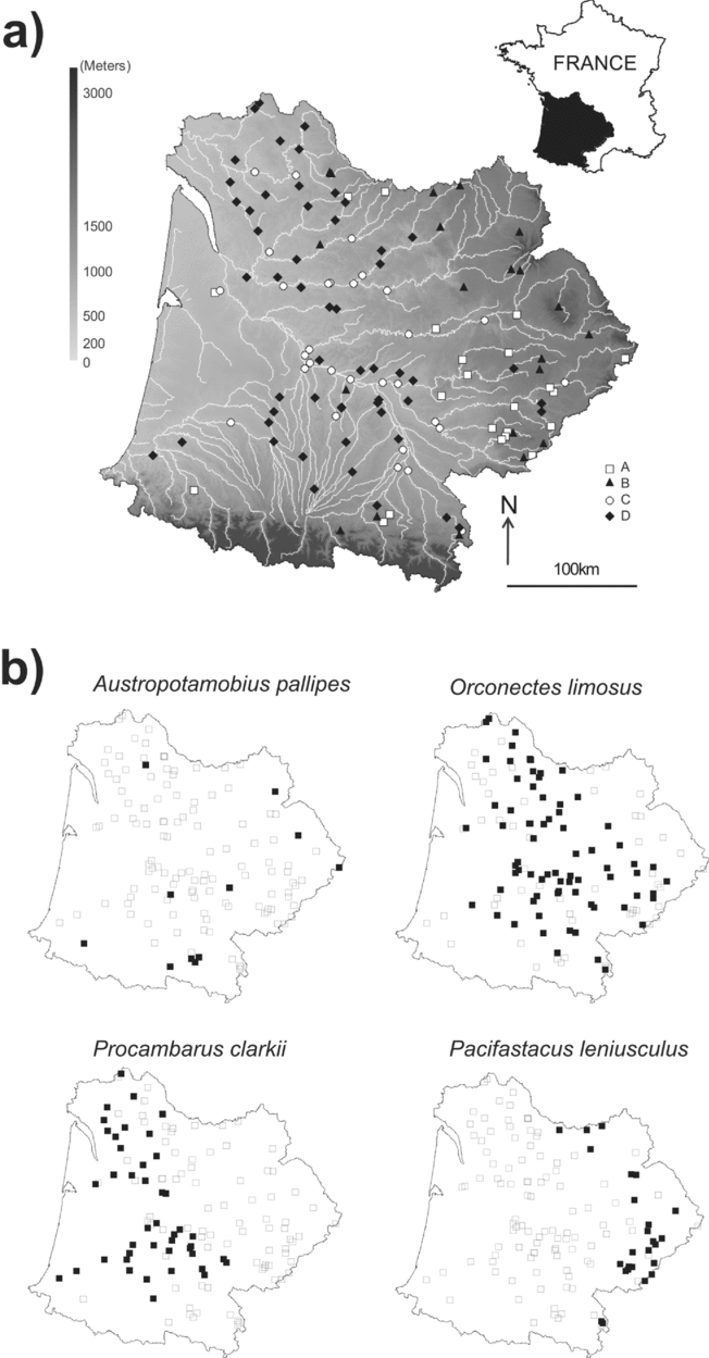
After training the SOM, the k-means algorithm helped to derive four clusters, based on the minimum Davies Bouldin Index (DBI = 1.0465, 0.9684, 0.8486 and 1.0012 for a solution with 2, 3, 4 and 5 clusters, respectively). Thus, sampling sites were classified into four subsets according to eight environmental variables (Fig. 1). Clusters were plotted on a geographical map of the Adour-Garonne Basin in order to ease interpretations (Fig. 2).
Distribution of the sampling sites on the self-organizing map (SOM). Codes correspond to sampling sites. Sites that are neighbours on the grid are expected to be similar in terms of environmental variables, and similarities decrease as sites are increasingly distant.

(a) Map of the Adour-Garonne stream system. Distribution of the 128 sampling sites and correspondence with their location (clusters) on the Kohonen map (see also Fig. 1). (b) Distribution maps for the four crayfish species. Filled squares denote locations where species are present, white squares denote locations where they are absent.

Sites in clusters A and B corresponded to headwater streams located at higher altitudes (Fig. 1). Within this frame, cluster A was delineated by higher proportions of forested areas (Fig. 3), while cluster B was characterized by steeper slopes and lower summer temperatures. Sites in cluster C were located in urban landscapes and were characterized by higher air temperature, high distance from the source and the largest drainage basin area (Fig. 3). Finally, sites in cluster D were located at low elevation, and primarily corresponded to agricultural areas (Fig. 3). When the distribution of species was visualized on the trained SOM using a shading scale (Fig. 4), headwater streams (clusters A and B) showed the highest probability of occurrence of the native crayfish Austropotamobius pallipes and the introduced species Pacifastacus leniusculus. Distribution maps (Fig. 2) showed that P. leniusculus occurred in the eastern part of the stream system (Massif Central mountains), while A. pallipes was rather found at few sites in the eastern Massif Central and southern areas (Pyrenées Mountains) of the drainage basin. It also appeared from the SOM analysis that A. pallipes was more likely to occur at sites located in forested areas or having steeper slopes, while P. leniusculus showed preferences for sites located at higher elevations and characterized by the lowest air temperatures. The units on the left bottom area (cluster C, urban landscapes) had highest probabilities of hosting Orconectes limosus (see also Fig. 2). The units on the right bottom corner (cluster D, agricultural areas) had high probability values for Procambarus clarkii.
Gradient analysis of each variable on the trained SOM, with visualization in shading scale (dark = high values, light = low values). Each individual map is to be compared with, or superimposed onto, the map in Figure 1.

Gradient analysis of the probability of occurrence of each crayfish species on the trained SOM (see Fig. 1), with visualization in shading scale (dark = high probability of occurrence, light = low probability of occurrence). Each individual map is to be compared with, or superimposed onto, the maps in Figures 1 and 3.

DISCUSSION
The complex relationships between the spatial heterogeneity of physical conditions, and the local to regional distributions of target species have often been studied through correlative techniques (Jongman et al. Reference Jongman, Braak and Tongeren1995). Other authors have taken into account habitat variability, by considering the proportional use of particular habitats among the available ones (Hastie et al. Reference Hastie, Boon and Young2000), but this approach is rather suited to the modelling of mesohabitat preferences on a local scale. However, the need for quantitative data, collected in a standardized manner, is a pre-requisite for the use of correlative techniques and habitat modelling. The SOM algorithm (Kohonen Reference Kohonen1982) is a heuristic model used to visualize and explore linear and non-linear relationships in high-dimensional datasets. SOMs were first used in the 1980s in speech recognition (Kohonen et al. Reference Kohonen, Mäkisara and Saramäki1984). Since Chon et al. (Reference Chon, Park, Moon and Cha1996) first applied the SOM to pattern benthic communities in streams, SOMs have been implemented in various aspects of water research, such as classifying biological and environmental data (Gevrey et al. Reference Gevrey, Rimet, Park, Giraudel, Ector and Lek2004; Tison et al. Reference Tison, Giraudel, Coste, Park and Delmas2004) and patterning long-term data (Kangur et al. Reference Kangur, Park, Kangur, Kangur and Lek2007). Although the SOM visualization is an indirect gradient analysis like a principal component analysis, SOMs can be used as an analysis tool to establish the relationships between sampling sites, and environmentaland biological variables. The advantages of the SOM in comparison with conventional multivariate analyses have been established (Gevrey et al. Reference Gevrey, Dimopoulos and Lek2003). In adding to the calculation of occurrence probabilities using binary data, it is important to highlight one of the most innovative applications of the SOM for conservation issues: the possibility of introducing a set of variables (for example biological variables) into a SOM that has been previously trained with other variables (for example environmental variables). This application, which enables researchers to tease out the relationships between two sets of variables, is convenient to examine the fit between species and their environment (as detailed in Céréghino & Park Reference Céréghino and Park2009). In this context, the SOM further maximizes the information extracted from large species matrices made of occurrence data, by transforming binary values into probabilities of presence, then allowing the comparison of environmental gradients and the likelihood that species will occur. Comparison among closely related species can also be made; any species association can be indicated by overlapping several maps. Thus, this approach can better analyse relationships between variables than general indirect gradient analysis.
The model probabilities of presence of native A. pallipes showed good agreement with current distributions at the watershed scale. In many European countries, the white-clawed crayfish is one of the most widespread decapod crustaceans (Holdich Reference Holdich2002), but both species distribution and population densities have drastically declined during the last decade (Gil-Sánchez & Alba-Tercedor Reference Gil-Sánchez and Alba-Tercedor2006). At the catchment scale, populations are scarce and reduced to marginal areas of stream systems, which are often disconnected from the main stream (Gil-Sánchez & Alba-Tercedor Reference Gil-Sánchez and Alba-Tercedor2002; Bramard et al. Reference Bramard, Demers, Trouilhé, Bachelier, Dumas, Fournier, Broussard, Robin, Souty-Grosset and Grandjean2006). Such observations reveal that some river sections remain more suitable than others in terms of habitat conditions, and this pattern was clearly illustrated in our study by differences in probabilities of presence among neighbouring sites within the stream system. However, as it is often reported, A. pallipes populations appeared to be mostly confined to headwater streams (i.e. colder waters), almost certainly because exotic competitors were unable to withstand the colder conditions that prevail in mountainous areas (Gil-Sánchez & Alba-Tercedor Reference Gil-Sánchez and Alba-Tercedor2002; Legalle et al. Reference Legalle, Mastrorillo and Céréghino2008). Introduced crayfish usually grow faster, have a greater size and less restricted habitat requirements than native species (Changeux Reference Changeux2003; Dunn et al. Reference Dunn, McClymont, Christmas and Dunn2009). Such ecological advantages are detrimental to the partition of habitat and food resource, and native populations subjected to antagonistic interactions with such species may rapidly decline to extinction (Gil-Sánchez & Alba-Tercedor Reference Gil-Sánchez and Alba-Tercedor2006). Moreover, foreign species may be predators on native species, and/or may be vectors of diseases (Moyle & Light Reference Moyle and Light1996; Gozlan et al. Reference Gozlan, Peeler, Longshaw, St-Hilaire and Feist2006). This problem typically affects the white-clawed crayfish. The introduction of Orconectes limosus, Pacifastacus leniusculus and Procambarus clarkii (among others) was the main reason for the decline of A. pallipes in the downstream sections of European rivers, as it led to a competitive exclusion of native crayfish (Vorburger & Ribi Reference Vorburger and Ribi1999; Dunn et al. Reference Dunn, McClymont, Christmas and Dunn2009), and brought the crayfish plague caused by the fungus Aphanomyces astaci (Kozubiková et al. Reference Kozubiková, Petrusek, Ďuriš, Martin, Diéguez-Uribeondo and Oidtmann2008).
Although A. pallipes and P. leniusculus had quite distinct geographic distributions (Fig. 2b), they showed rather similar preferences for local environments. Gradient distributions for P. leniusculus (Fig. 4) could be perceived as a negative picture of the gradient depicting the distribution of A. pallipes. Our analyses suggest that A. pallipes and P. leniusculus have different preferences within a common range of headwater environments for certain variables such as slope and land cover. Conversely, such a pattern also suggests that competitive exclusion occurs within the stream system, and that subsequent competition with the exotic species P. leniusculus is a key factor explaining the current distribution of A. pallipes within the stream system. P. leniusculus is indeed recognized as the principal competitor of A. pallipes (Changeux Reference Changeux2003; Bramard et al. Reference Bramard, Demers, Trouilhé, Bachelier, Dumas, Fournier, Broussard, Robin, Souty-Grosset and Grandjean2006). This highly invasive species commonly leads to the displacement of native A. pallipes. According to probabilities of occurrence, Procambarus clarkii and Orconectes limosus had distinct distributions that showed little spatial overlap with any other species. Procambarus clarkii is well adapted to life in agricultural areas; translocations have been most successful in agricultural areas employing irrigation systems (Hobbs et al. Reference Hobbs, Jass and Huner1989). In Spain, this species has severe impacts on rice agriculture (Cruz & Rebelo Reference Cruz and Rebelo2007), while in France, it often occurs in marshy and rice areas (Bramard et al. Reference Bramard, Demers, Trouilhé, Bachelier, Dumas, Fournier, Broussard, Robin, Souty-Grosset and Grandjean2006). Although P. clarkii is often described as a competitor of A. pallipes, our results show that its habitat preferences differ from those of A. pallipes, resulting in a spatial segregation of the species. In fact, P. clarkii seems to be unable to colonize mountainous headwater streams where A. pallipes has found refuge (Gil-Sanchez & Alba-Tercedor Reference Gil-Sánchez and Alba-Tercedor2002). Orconectes limosus occurs in urbanized areas corresponding to lower elevation streams. In the other European countries, the American spiny-cheek crayfish (O. limosus) is also mainly found in lower reaches of watercourses (Petrusek et al. Reference Petrusek, Filipová, Ďuriš, Horká, Kozák, Policar, Štambergová and Kučera2006) or in large lakes (Schulz et al. Reference Schulz, Smietana and Schulz2002) and does not penetrate far upstream. Its distribution in standing waters is largely the result of intentional human-mediated translocations (Petrusek et al. Reference Petrusek, Filipová, Ďuriš, Horká, Kozák, Policar, Štambergová and Kučera2006) and reflects the intensity of human activities (Schulz et al. Reference Schulz, Smietana and Schulz2002).
Manel et al. (Reference Manel, Dias, Buckton and Ormerod1999) demonstrate that the overall success of prediction of ANNs is superior to that of logistic regression and discriminant analyses when predicting the presence or absence of river birds according to the environmental variables. ANN predictions outperformed logistic regression, linear discriminant analysis and classifications trees approaches for predicting fish species presence/absence (Olden & Jackson Reference Olden and Jackson2002). ANNs present major advantages where species-environment links cannot be transformed to linearity (Lek et al. Reference Lek, Delacoste, Baran, Dimopoulos, Lauga and Aulagnier1996) and offer an alternative to traditional statistical methods for classifying complex data. Moreover, ANNs are not dependent on particular relationships, need no assumptions regarding underlying data distributions and no a priori understanding of variable relationships (Olden & Jackson Reference Olden and Jackson2001). This independence from assumptions makes ANNs a powerful option for exploring complex potential non-linear relationships such as the associations between animal species and their environment (Joy & Death Reference Joy and Death2004). ANNs also allowed a single model to predict the entire considered assemblage in one procedure (Joy & Death Reference Joy and Death2004). Studies involving predictive modeling of species occurrence increasingly combine the power of GIS with multivariate statistical tools to formalize the link between species and their environment and to enhance the potential to create accurate predictive models (Joy & Death Reference Joy and Death2004). In this study, the predictions from the ANN using land cover information (obtained from GIS) and simple environmental data showed that SOMs are a valuable technique to forecast crayfish distributions. This technique yields a clear bidimensional projection of a relatively large volume of site-specific data on species occurrences and then allows their interpretation in terms of occurrence probabilities of species in different geographic areas. Moreover, by overlapping various species maps (for example Fig. 4), any spatial overlap or segregation of the different species become clear. Most surveillance techniques for aquatic aliens use extensive numbers of site-specific data to allow predictions of the distribution of species in a given area, using a set of environmental variables (Ricciardi & Rasmussen Reference Ricciardi and Rasmussen1998). The SOM visualization can be used as an analytical tool to bring out relationships between sample locations, biological variables and the occurrence of each species. Our study demonstrates the association of two modelling tools (GIS and neural networks) could improve ecological risk assessments;the techniques may have many potential uses, notably to identify areas in need for protection or areas suitable for reintroduction of endangered species such as the white-clawed A. pallipes.
ACKNOWLEDGEMENTS
We thank the Onema (Office National de l'Eau et des Milieux Aquatiques) for provision of the database, and the Fédération de Pêche du Lot, Agence de l'Eau Adour-Garonne, Conseil Régional Midi-Pyrénées, Conseil Général du Lot, Fédération Nationale pour la Pêche en France, EDF (contract: N°08005117) for funding. Two anonymous reviewers provided helpful comments on an earlier version of this paper.