







1. Introduction
The prediction and low-order reconstruction of flow patterns are important topics for fundamental research of turbulence as well as engineering applications. The physics-based approaches (Hwang & Cossu Reference Hwang and Cossu2010b; McKeon & Sharma Reference McKeon and Sharma2010) utilise the linearised Navier–Stokes (LNS) equations that govern the flow dynamics to analyse the dominant coherent flow motions. In these approaches, the Navier–Stokes equations are written as linear evolution equations with nonlinear forcing as feedback, which drives the dynamic system (McKeon Reference McKeon2017). On the other hand, the fluctuations of the flow state, such as velocities, pressure and temperature, are defined as the responses of the dynamic system. The dynamic patterns of the flow system are determined by the energy amplification and redistribution mechanisms, which are described by the linear operator and the nonlinear forcing (Morra et al. Reference Morra, Nogueira, Cavalieri and Henningson2021).
When the linearised formulations of the Navier–Stokes equations are built at a given spatiotemporal scale, the linear operator that links the response and nonlinear forcing is referred to as the resolvent (McKeon & Sharma Reference McKeon and Sharma2010; Sharma & McKeon Reference Sharma and McKeon2013). Taking singular value decomposition (SVD) to the resolvent operator, the response and forcing modes are obtained, which are ordered by their singular values. The resolvent analysis has been actively applied in turbulence studies by focusing on the leading response mode with the largest energy amplification, which captures the dominant flow structures (e.g. Moarref et al. Reference Moarref, Sharma, Tropp and McKeon2013; Sharma & McKeon Reference Sharma and McKeon2013; McKeon Reference McKeon2019). These studies bypass the need to model the nonlinear forcing based on the assumption of the low-rank behaviour, which is valid when the singular value of the leading mode is significantly larger than the subsequent modes (Pickering et al. Reference Pickering, Rigas, Schmidt, Sipp and Colonius2021). Meanwhile, the significant influence of the colour of forcing on the resultant responses is widely reported (Zare, Jovanović & Georgiou Reference Zare, Jovanović and Georgiou2017; Illingworth, Monty & Marusic Reference Illingworth, Monty and Marusic2018; Madhusudanan, Illingworth & Marusic Reference Madhusudanan, Illingworth and Marusic2019; Morra et al. Reference Morra, Semeraro, Henningson and Cossu2019).
To partially model the forcing colours, Del Alamo & Jiménez (Reference Del Alamo and Jiménez2006) introduced the eddy-viscosity model (Cess Reference Cess1958) that linearises a part of the input forcing, where the linear operator is correspondingly changed by adding the linearised eddy-viscosity term in the original operator. On the other hand, the unmodelled part of forcing remains to be assumed as uniform and uncorrelated in space. With the modified resolvent operator modelled by the eddy-viscosity term, the low-order models have improved alignments with the spectral proper orthogonal decomposition (SPOD) modes in the turbulent channel flow (Morra et al. Reference Morra, Semeraro, Henningson and Cossu2019; Symon et al. Reference Symon, Madhusudanan, Illingworth and Marusic2023; Zhu, Chen & Fu Reference Zhu, Chen and Fu2024) and jets (Pickering et al. Reference Pickering, Towne, Jordan and Colonius2020, Reference Pickering, Rigas, Schmidt, Sipp and Colonius2021). Here, the alignments between the resolvent and SPOD modes are utilised to assess the validity of the resolvent analysis quantitatively (Morra et al. Reference Morra, Semeraro, Henningson and Cossu2019; Pickering et al. Reference Pickering, Rigas, Schmidt, Sipp and Colonius2021; Symon et al. Reference Symon, Madhusudanan, Illingworth and Marusic2023; Fan et al. Reference Fan, Kozul, Li and Sandberg2024) since the leading SPOD mode extracts the most energetic spatiotemporally coherent structures (Lumley Reference Lumley1967, Reference Lumley2007; Schmidt et al. Reference Schmidt, Towne, Rigas, Colonius and Brès2018). Meanwhile, the eddy-viscosity model (e.g. Cess Reference Cess1958) is based on the relationship between the Reynolds stress and mean shear rate of strain rather than the fluctuation variables investigated in the resolvent analysis. In Hwang (Reference Hwang2016), the mechanism of the eddy-viscosity model in the linear analysis of turbulence is attributed to the fact that the eddy viscosity mimics the nonlinear interactions in the process of energy cascade and turbulent dissipation. In the near-wall region, the dissipation mechanism is dominated by the molecular viscosity. Meanwhile, due to the large separation between the integral scale and dissipation scale in the outer region, the turbulent dissipation should be vigorous. The spatial distribution of the eddy viscosity (Cess Reference Cess1958) matches well with the above patterns, which explains its success in predicting the optimal transient growth of small organised perturbations. Symon, Illingworth & Marusic (Reference Symon, Illingworth and Marusic2021) analyse the nonlinear transfer modelled by the eddy-viscosity term, finding that the leading resolvent mode successfully identifies the main production mechanisms in the flow. Kuhn, Soria & Oberleithner (Reference Kuhn, Soria and Oberleithner2021) quantitatively investigated the turbulent production in linear modelling of turbulent jet flow. In Symon et al. (Reference Symon, Madhusudanan, Illingworth and Marusic2023), it was demonstrated that the accuracy of the eddy-viscosity model relies on striking the right balance between the positive and negative energy transfers. On the other hand, in Hwang & Cossu (Reference Hwang and Cossu2010b) and Alizard et al. (Reference Alizard, Pirozzoli, Bernardini and Grasso2015), the role of the eddy viscosity in modelling the fluctuation of nonlinear terms is explained via the triple decomposition (Hussain & Reynolds Reference Hussain and Reynolds1970; Reynolds & Hussain Reference Reynolds and Hussain1972). According to Chen et al. (Reference Chen, Cheng, Gan and Fu2023b) and Cheng et al. (Reference Cheng, Chen, Zhu, Shyy and Fu2024), the shear stress term of the (large-amplitude) unsteady component of the base flow is linearised with the organised wave under the Boussinesq assumption using the eddy viscosity. However, it is still ambiguous how the eddy-viscosity model works in modelling part of the fluctuating nonlinear terms to be the linear function of the fluctuation flow state.
The introduction of eddy-viscosity models also improves the physics-based estimation of turbulence (Illingworth et al. Reference Illingworth, Monty and Marusic2018; Madhusudanan et al. Reference Madhusudanan, Illingworth and Marusic2019; Martini et al. Reference Martini, Cavalieri, Jordan, Towne and Lesshafft2020; Towne, Lozano-Durán & Yang Reference Towne, Lozano-Durán and Yang2020; Amaral et al. Reference Amaral, Cavalieri, Martini, Jordan and Towne2021; Ying, Li & Fu Reference Ying, Li and Fu2024) with the LNS equations. In Illingworth et al. (Reference Illingworth, Monty and Marusic2018), the role of eddy viscosity was explained to model the influence of small-scale turbulent fluctuations on large-scale ones. It is found that the accuracy of the estimated large-scale motions from the modelled estimator is improved significantly. Towne et al. (Reference Towne, Lozano-Durán and Yang2020) utilise the eddy-viscosity-modelled resolvent operator to predict the space–time properties based on the measured information in the buffer layer. The predicted flow statistics in the near-wall region are consistent with the direct numerical simulation (DNS) results. The improvement of the estimation accuracy with the eddy-viscosity-modelled resolvent operator compared with that with the unmodelled one was also reported by Amaral et al. (Reference Amaral, Cavalieri, Martini, Jordan and Towne2021). Meanwhile, compared with the optimal linear estimation results informed by the real forcing statistics, the eddy-viscosity-modelled results still have substantially larger estimation errors (Amaral et al. Reference Amaral, Cavalieri, Martini, Jordan and Towne2021), which hinders the engineering applications of the resolvent-based estimations where the real forcing statistics are unavailable. Thus, the forcing models need to be further improved to enhance the practical values of the linear estimation of turbulence.
Since the treatments of the forcing term are found to have a significant effect on the results of the resolvent analysis and the physics-based estimations, the modelling strategy and fundamental research of forcing have drawn increasing interest. In addition to the eddy-viscosity models that are adopted by the literature mentioned above, there are also attempts to propose new eddy-viscosity models (Gupta et al. Reference Gupta, Madhusudanan, Wan, Illingworth and Juniper2021; Pickering et al. Reference Pickering, Rigas, Schmidt, Sipp and Colonius2021) or directly model the stochastic forcing defined as the remaining part of forcing after excluding the modelled part (Gupta et al. Reference Gupta, Madhusudanan, Wan, Illingworth and Juniper2021; Holford, Lee & Hwang Reference Holford, Lee and Hwang2023; Ying et al. Reference Ying, Liang, Li and Fu2023). Tissot, Cavalieri & Mémin (Reference Tissot, Cavalieri and Mémin2021) improved the prediction of the resolvent analysis by considering the stochastic interaction with the background turbulence via nonlinear energy redistribution. Pickering et al. (Reference Pickering, Rigas, Schmidt, Sipp and Colonius2021) optimised the eddy viscosity of turbulent jet flow by minimising the relative error between the leading resolvent and SPOD modes. On the other hand, Holford et al. (Reference Holford, Lee and Hwang2023) optimised the stochastic forcing according to the auto-spectra of the velocity fluctuations from the DNS data while using the mean-quantity-based eddy viscosity. Without the requirement of the DNS data in the near-wall region, Ying et al. (Reference Ying, Liang, Li and Fu2023) modelled the stochastic forcing by taking the resolvent-based near-wall prediction (Towne et al. Reference Towne, Lozano-Durán and Yang2020) of turbulent channel flow into consideration. Using the measurements from a horizontal layer lower than the upper bound of the logarithmic region, the predicted space–time properties of the near-wall velocities match well with the DNS results with  $Re_{\tau }=187$–
 $934$. Gupta et al. (Reference Gupta, Madhusudanan, Wan, Illingworth and Juniper2021) propose the scale-dependent model (
 $\lambda$-model), which simultaneously modifies the eddy viscosity and stochastic forcing profile based on the scaling of the energy-containing eddies in wall turbulence (Jiménez Reference Jiménez2012).
The studies focusing directly on the forcing in wall turbulence have been actively conducted in recent years (Morra et al. Reference Morra, Nogueira, Cavalieri and Henningson2021; Nogueira et al. Reference Nogueira, Morra, Martini, Cavalieri and Henningson2021; Karban et al. Reference Karban, Martini, Cavalieri, Lesshafft and Jordan2022). In Nogueira et al. (Reference Nogueira, Morra, Martini, Cavalieri and Henningson2021), the forcing statistics of turbulent Couette flow with  $Re_{\tau }=400$ are studied. Two representative energetic modes are specially focused on, i.e. mode with
 $(k_x/h,k_z/h)=(0,1)$ related to the streamwise vortices and streak, and mode
 $(k_x/h,k_z/h)=(1,0)$ related to spanwise-coherent fluctuations, where
 $h$ is the half-channel height. It is found that the response can be well reconstructed with a subset of forcing. Later, Morra et al. (Reference Morra, Nogueira, Cavalieri and Henningson2021) report the counteraction effect between the streamwise component of forcing and the remaining part. In Karban et al. (Reference Karban, Martini, Cavalieri, Lesshafft and Jordan2022), the self-similar structures of forcing are revealed, finding that both the estimated forcing from the resolvent-based estimation with wall measurements and that correlated to the wall shear stress show self-similar behaviours.
In the above-reviewed studies, the mechanisms of eddy-viscosity terms in linear analysis of turbulence were preliminarily explored (Hwang Reference Hwang2016; Symon et al. Reference Symon, Madhusudanan, Illingworth and Marusic2023). Such mechanism still remains to be clarified after several existing studies on the forcing statistics (Morra et al. Reference Morra, Nogueira, Cavalieri and Henningson2021; Nogueira et al. Reference Nogueira, Morra, Martini, Cavalieri and Henningson2021), where the clarification of the effect of the interactions of the forcing and eddy-viscosity terms on the resultant stochastic forcing and response is somehow absent. To date, the mean-quantity-based eddy viscosity is still widely used in the linear analysis of turbulence on an ad hoc basis (e.g. Zhu et al. Reference Zhu, Chen and Fu2024). In this study, the underlying mechanism of the eddy viscosity in the linear analysis of turbulence is investigated through the statistical properties of the forcing and eddy-viscosity terms, based on which an effective optimisation framework of the eddy viscosity is constructed. Further, a predictive eddy-viscosity model is developed based on the characteristics of the optimised eddy viscosity.
The remainder of this article is organised as follows. In § 2, the linearisation of the incompressible Navier–Stokes equations and the concept of SPOD are described, followed by the relationship between the resolvent and SPOD modes. The mechanisms of the eddy viscosity in the linear analysis of turbulence are investigated with the DNS results in § 3. In § 4, an optimisation framework of the eddy-viscosity profiles is proposed and validated. A new predictive eddy-viscosity model is then constructed based on the optimised results. Discussion and concluding remarks are provided in § 5.
2. Methodology
2.1. Linearisation of the incompressible Navier–Stokes equations
The incompressible Navier–Stokes equations are given by
 $$\begin{gather} \frac{\partial \boldsymbol{u}}{\partial t}+\boldsymbol{u}\boldsymbol{\cdot}\boldsymbol{\nabla}\boldsymbol{u} ={-}\boldsymbol{\nabla} p+\frac{1}{Re_\tau}\boldsymbol{\nabla}\boldsymbol{\cdot}(\boldsymbol{\nabla}\boldsymbol{u}+\boldsymbol{\nabla}\boldsymbol{u}^{\rm T}), \end{gather}$$
 $$\begin{gather}\boldsymbol{\nabla}\boldsymbol{\cdot}\boldsymbol{u} = 0, \end{gather}$$
where  $Re_\tau = {u_{\tau } h}/{\nu }$ is the friction Reynolds number,
 $u_{\tau }$ is the friction velocity,
 $\nu$ is the kinetic viscosity and superscript T denotes transpose. By rearranging (2.1), the LNS equations for fluctuating velocity
 $\boldsymbol {u}^\prime$ and pressure
 $p^\prime$ hold as
 $$\begin{gather} \frac{\partial \boldsymbol{u}^\prime}{\partial t}+ U \boldsymbol{\cdot}\boldsymbol{\nabla}\boldsymbol{u}^\prime +\boldsymbol{u}^\prime\boldsymbol{\cdot}\boldsymbol{\nabla} U + \boldsymbol{\nabla} p^\prime -\frac{1}{Re_\tau}\boldsymbol{\nabla}\boldsymbol{\cdot}[(\boldsymbol{\nabla}\boldsymbol{u}^\prime+{\boldsymbol{\nabla}\boldsymbol{u}^\prime}^{\rm T})] = \boldsymbol{f}^{\prime}, \end{gather}$$
 $$\begin{gather}\boldsymbol{\nabla}\boldsymbol{\cdot}\boldsymbol{u}^\prime = 0, \end{gather}$$
where  $U$ is the mean velocity. The forcing
 $\boldsymbol {f}^{\prime }$ that contains the nonlinear interactions of velocity fluctuations is defined as
 \begin{equation} \boldsymbol{f}^{\prime}={-}\left(\boldsymbol{u}^\prime\boldsymbol{\cdot}\boldsymbol{\nabla}\boldsymbol{u}^\prime - \left\langle \boldsymbol{u}^\prime\boldsymbol{\cdot}\boldsymbol{\nabla}\boldsymbol{u}^\prime\right\rangle\right), \end{equation}
where  $\langle ~ \rangle$ denotes time average.
When considering modelling the forcing term with eddy viscosity, the eddy-viscosity- based linearised Navier–Stokes (eLNS) equations hold as
 $$\begin{gather} \displaystyle\frac{\partial \boldsymbol{u}^\prime}{\partial t}+ U \boldsymbol{\cdot}\boldsymbol{\nabla}\boldsymbol{u}^\prime +\boldsymbol{u}^\prime\boldsymbol{\cdot}\boldsymbol{\nabla} U +\boldsymbol{\nabla} p^\prime -\frac{1}{Re_\tau}\boldsymbol{\nabla}\boldsymbol{\cdot}\left[\frac{\nu_{m}+\nu}{\nu}(\boldsymbol{\nabla}\boldsymbol{u}^\prime+{\boldsymbol{\nabla}\boldsymbol{u}^\prime}^{\rm T})\right]= \boldsymbol{d}^{\prime}, \end{gather}$$
 $$\begin{gather}\boldsymbol{\nabla}\boldsymbol{\cdot} \boldsymbol{u}^\prime = 0, \end{gather}$$
where  $\nu _{m}$ is the eddy kinetic viscosity, and the stochastic forcing
 $\boldsymbol {d}^{\prime }$ is defined as
 \begin{equation} \boldsymbol{d}^{\prime} = \boldsymbol{f}^{\prime} - \boldsymbol{e}^{\prime}, \end{equation}
where  $\boldsymbol {e}^{\prime }=({1}/{Re_\tau })\boldsymbol {\nabla }\boldsymbol {\cdot }[{\nu _{m}}/{\nu }(\boldsymbol {\nabla }\boldsymbol {u}^\prime +{\boldsymbol {\nabla }\boldsymbol {u}^\prime }^{\rm T})]$ is the eddy-viscosity term.
Taking the Fourier transformation to (2.4) in the homogeneous spatial directions, the LNS equations in each spatial scale  $\boldsymbol {k}_{s}$ are obtained. Denoting
 $x(x_1)$,
 $y(x_2)$ and
 $z(x_3)$ as the streamwise, wall-normal and spanwise coordinates, respectively, the Fourier transformation is taken in
 $x$ and
 $z$ directions for the fully developed turbulent channel flow with
 $\boldsymbol {k}_{s} = (k_x , k_z)$. To eliminate the pressure term, the standard conversion (Jovanovic & Bamieh Reference Jovanovic and Bamieh2001) is applied, where the state is determined by the wall-normal velocity
 $(v)$ and vorticity
 $(\eta = \partial _z u - \partial _x w)$ fluctuations. Consequently, the evolution equation of the dynamic system with input
 $\hat {\boldsymbol {d}}_{\boldsymbol {k}_{s}}(t)$ and output
 $\hat {\boldsymbol {u}}_{\boldsymbol {k}_{s}}(t)$ is expressed as
 $$\begin{gather} \frac{\partial \hat{\boldsymbol{q}}_{\boldsymbol{k}_{s}}(t)}{\partial t} = {{\boldsymbol{\mathsf{A}}}}_{\boldsymbol{k}_{s}}\hat{\boldsymbol{q}}_{\boldsymbol{k}_{s}}(t) + {{\boldsymbol{\mathsf{B}}}}_{\boldsymbol{k}_{s}}\hat{\boldsymbol{d}}_{\boldsymbol{k}_{s}}(t), \end{gather}$$
 $$\begin{gather}\hat{\boldsymbol{u}}_{\boldsymbol{k}_{s}}(t) = {{\boldsymbol{\mathsf{C}}}}_{\boldsymbol{k}_{s}}\hat{\boldsymbol{q}}_{\boldsymbol{k}_{s}}(t), \end{gather}$$
where the state  $\hat {\boldsymbol {q}}_{\boldsymbol {k}_{s}}(t) = [\hat {v} , \hat {\eta }]^{\rm T}$ and the superscript
 ${}^{\ast }$ denotes the Hermitian transpose. The operators
 ${{\boldsymbol{\mathsf{A}}}}_{\boldsymbol {k}_{s}}$ and
 ${{\boldsymbol{\mathsf{B}}}}_{\boldsymbol {k}_{s}}$ are defined as
 \begin{align} {{\boldsymbol{\mathsf{A}}}}_{\boldsymbol{k}_{s}}= \left[ \begin{array}{@{}cc@{}} \varDelta^{{-}1}\mathscr{L}_{\mathscr{OS}} & 0 \\ -{\rm i} k_z U^{y} & \mathscr{L}_{\mathscr{SQ}} \end{array} \right],\quad {{\boldsymbol{\mathsf{B}}}}_{\boldsymbol{k}_{s}}= \left[\begin{array}{ccc} -{\rm i}k_x \varDelta^{{-}1} \mathscr{D} & -k^2 \varDelta^{{-}1} & {\rm i} k_z \varDelta^{{-}1} \mathscr{D}\\ {\rm i} k_z & 0 & -{\rm i} k_x \end{array} \right]_{\vphantom{A_A}}, \end{align}
where  $\varDelta = \mathscr {E}-k^2$,
 $k^2 = k_x^2 + k_z^2$, the operator
 $\mathscr {D}$ and superscript
 ${}^{y}$ both denote
 ${\partial }/{\partial y}$, and the Orr–Sommerfeld operator
 $\mathscr {L}_{\mathscr {OS}}$ and Squire operator
 $\mathscr {L}_{\mathscr {SQ}}$ are defined by (Hwang & Cossu Reference Hwang and Cossu2010b)
 \begin{equation} \left.\begin{gathered} \mathscr{L}_{\mathscr{OS}} ={-}{\rm i} k_x \left( U \varDelta - U^{yy} \right) + (\nu+\nu_{m}) \varDelta^2 + 2\nu_{m}^{y}\Delta\mathscr{D}+ \nu_{m}^{yy}(\mathscr{E}+k^2),\\ \mathscr{L}_{\mathscr{SQ}} ={-}{\rm i} k_x U + (\nu+\nu_{m}) \varDelta + \nu_{m}^{y}\mathscr{D}, \end{gathered}\right\} \end{equation}
respectively, where the operator  $\mathscr {E}$ and superscript
 ${}^{yy}$ both denote
 $\partial ^2/\partial ^2y$. The original velocity fluctuation
 $\hat {\boldsymbol {u}}_{\boldsymbol {k}_{s}}(t)$ is retrieved from
 $\hat {\boldsymbol {q}}_{\boldsymbol {k}_{s}}(t)$ via (2.6b), where the output matrix
 ${{\boldsymbol{\mathsf{C}}}}_{\boldsymbol {k}_{s}}$ is expressed as
 \begin{equation} {{\boldsymbol{\mathsf{C}}}}_{\boldsymbol{k}_{s}}=\frac{1}{k^2}\left[ \begin{array}{@{}cc@{}} {\rm i} k_x \mathscr{D} & -{\rm i} k_z \\ k^2 & 0 \\ {\rm i} k_z \mathscr{D} & {\rm i} k_x \end{array} \right]. \end{equation}
Equation (2.6) of the dynamic system can be further Fourier-transformed in the temporal ( $t$) direction when the system achieves statistically stationary in the temporal direction at each spatial location. The LNS equations at each spatiotemporal scale
 $\boldsymbol {k} = (\boldsymbol {k}_{s},\omega )$ is expressed as
 \begin{equation} \hat{\boldsymbol{u}}_{\boldsymbol{k}} = {{\boldsymbol{\mathsf{H}}}}_{\boldsymbol{k}} \boldsymbol{\cdot} \hat{\boldsymbol{d}}_{\boldsymbol{k}}, \end{equation}
where the transfer function
 \begin{equation} {{\boldsymbol{\mathsf{H}}}}_{\boldsymbol{k}} = {{\boldsymbol{\mathsf{C}}}}_{\boldsymbol{k}_{s}} \boldsymbol{\cdot} {{\boldsymbol{\mathsf{R}}}}_{\boldsymbol{k}} \boldsymbol{\cdot} {{\boldsymbol{\mathsf{B}}}}_{\boldsymbol{k}_{s}}, \end{equation}
 ${{\boldsymbol{\mathsf{R}}}}_{\boldsymbol {k}} = ( \textrm {i}\omega {{\boldsymbol{\mathsf{I}}}} - {{\boldsymbol{\mathsf{A}}}}_{\boldsymbol {k}_{s}} )^{-1}$ is the resolvent of
 ${{\boldsymbol{\mathsf{A}}}}_{\boldsymbol {k}_{s}}$,
 $\textrm {i} = \sqrt {-1}$ and
 ${{\boldsymbol{\mathsf{I}}}}$ is the identity matrix. Here, we define the inner product of variables
 $\boldsymbol {a}$ and
 $\boldsymbol {b}$ as
 \begin{equation} \lbrace \boldsymbol{a} , \boldsymbol{b} \rbrace =\boldsymbol{a}^{{\ast}} \boldsymbol{\cdot} {{\boldsymbol{\mathsf{W}}}} \boldsymbol{\cdot} \boldsymbol{b}, \end{equation}
where  ${{\boldsymbol{\mathsf{W}}}}$ is a diagonal matrix that accounts for the energy norm. Taking SVD to the transfer function
 ${{\boldsymbol{\mathsf{H}}}}_{\boldsymbol {k}}$ considering the energy norm, the following relationship holds:
 \begin{equation} \tilde{{{\boldsymbol{\mathsf{H}}}}}_{\boldsymbol{k}} = \tilde{{\varPsi}}_{\boldsymbol{k}} \boldsymbol{\cdot} \boldsymbol{\varSigma}_{\boldsymbol{k}} \boldsymbol{\cdot} \tilde{\varPhi}_{\boldsymbol{k}}^{{\ast}}, \end{equation}
where  $\tilde {{{\boldsymbol{\mathsf{H}}}}}_{\boldsymbol {k}}={{\boldsymbol{\mathsf{W}}}}^{1/2} \boldsymbol {\cdot }{{\boldsymbol{\mathsf{H}}}}_{\boldsymbol {k}} \boldsymbol {\cdot }{{\boldsymbol{\mathsf{W}}}}^{-1/2}$,
 $\tilde {{\varPsi }}_{\boldsymbol {k}}={{\boldsymbol{\mathsf{W}}}}^{1/2} \boldsymbol {\cdot } \varPsi _{\boldsymbol {k}}$ and
 $\tilde {{\varPhi }}_{\boldsymbol {k}}={{\boldsymbol{\mathsf{W}}}}^{1/2} \boldsymbol {\cdot } \varPhi _{\boldsymbol {k}}$. The resolvent response modes
 $\boldsymbol {\psi }_{\boldsymbol {k},i}$, forcing modes
 $\boldsymbol {\phi }_{\boldsymbol {k},i}$ and singular values
 $\sigma _{\boldsymbol {k},i}$ are assembled as
 $\varPsi _{\boldsymbol {k}} = [\boldsymbol {\psi }_{\boldsymbol {k},1} , \boldsymbol {\psi }_{\boldsymbol {k},2} ,\ldots ]$,
 $\varPhi _{\boldsymbol {k}} = [\boldsymbol {\phi }_{\boldsymbol {k},1} , \boldsymbol {\phi }_{\boldsymbol {k},2} ,\ldots ]$ and
 $\boldsymbol {\varSigma }_{\boldsymbol {k}} = \textrm {diag}[\sigma _{\boldsymbol {k},1} , \sigma _{\boldsymbol {k},2} ,\ldots ]$, respectively. The resolvent modes are ordered by the singular values, which means that the first one reflects the most amplified shape with respect to the given energy of the corresponding forcing mode.
Further defining the expansion coefficient
 \begin{equation} \boldsymbol{\beta}_{\boldsymbol{k}} = \hat{\boldsymbol{d}}_{\boldsymbol{k}}^{{\ast}} \boldsymbol{\cdot} {{\boldsymbol{\mathsf{W}}}} \boldsymbol{\cdot} \varPhi_{\boldsymbol{k}}, \end{equation}
whose physical meaning is the projection of the actual stochastic forcing  $\hat {\boldsymbol {d}}_{\boldsymbol {k}}$ onto the orthonormal forcing modes (McKeon Reference McKeon2017), the resolvent formulation (2.10) can be rewritten as
 \begin{equation} \hat{\boldsymbol{u}}_{\boldsymbol{k}} = {\varPsi}_{\boldsymbol{k}} \boldsymbol{\cdot} \boldsymbol{\varSigma}_{\boldsymbol{k}} \boldsymbol{\cdot} \boldsymbol{\beta}_{\boldsymbol{k}} = \sum_i \sigma_{\boldsymbol{k},i} \beta_{\boldsymbol{k},i} \boldsymbol{\psi}_{\boldsymbol{k},i}. \end{equation}
From (2.15), the response  $\hat {\boldsymbol {u}}_{\boldsymbol {k}}$ can be interpreted as the linear summation of all the response modes weighted by the product of
 $\beta _{\boldsymbol {k},i}$ and
 $\sigma _i$. To conduct the resolvent analysis in this study, the mean velocity profiles from the DNS are utilised to construct the linear operator.
The linearised equations are discretised in the wall-normal direction with the same settings as the DNS that will be introduced in § 3.1, which avoids interpolation of the mean velocity profiles onto different grids. The boundary conditions of  $\hat {v}=0$,
 $\partial {\hat {v}}/\partial {y} = 0$ and
 $\hat {\eta } = 0$ at the walls on both sides of the channel, i.e.
 $y/h = 0$ and
 $2$, are imposed here.
2.2. SPOD
The SPOD finds the deterministic function that best approximates a zero-mean stochastic process at each spatiotemporal scale (Lumley Reference Lumley1967; Berkooz, Holmes & Lumley Reference Berkooz, Holmes and Lumley1993; Towne, Schmidt & Colonius Reference Towne, Schmidt and Colonius2018). Defining the cross-spectral density (CSD) tensor at a given spatiotemporal scale  $\boldsymbol {k}$, i.e.
 \begin{equation} {{\boldsymbol{\mathsf{S}}}}_{\boldsymbol{uu},\boldsymbol{k}} = \left\langle{\hat{\boldsymbol{u}}_{\boldsymbol{k}} \boldsymbol{\cdot} \hat{\boldsymbol{u}}_{\boldsymbol{k}}^{{\ast}}}\right\rangle, \end{equation}
the SPOD modes can be obtained by taking eigendecomposition on the CSD tensor considering the energy norm, i.e.
 \begin{equation} \tilde{{{\boldsymbol{\mathsf{S}}}}}_{\boldsymbol{uu},\boldsymbol{k}} = \tilde{{{\boldsymbol{\mathsf{U}}}}}_{\boldsymbol{k}} \boldsymbol{\cdot} \boldsymbol{\varLambda}_{\boldsymbol{k}} \boldsymbol{\cdot} \tilde{{{\boldsymbol{\mathsf{U}}}}}_{\boldsymbol{k}}^{{\ast}}, \end{equation}
where  $\tilde {{{\boldsymbol{\mathsf{S}}}}}_{\boldsymbol {uu},\boldsymbol {k}}={{\boldsymbol{\mathsf{W}}}}^{1/2} \boldsymbol {\cdot } {{\boldsymbol{\mathsf{S}}}}_{\boldsymbol {uu},\boldsymbol {k}} \boldsymbol {\cdot } {{\boldsymbol{\mathsf{W}}}}^{1/2}$,
 $\tilde {\boldsymbol {U}}_{\boldsymbol {k}}={{\boldsymbol{\mathsf{W}}}}^{1/2} \boldsymbol {\cdot } \boldsymbol {U}_{\boldsymbol {k}}$. The tensor
 ${{\boldsymbol{\mathsf{U}}}}_{\boldsymbol {k}} = [{\boldsymbol{\mathscr{u}}}_{\boldsymbol {k},1} , \boldsymbol{\mathscr{u}}_{\boldsymbol {k},2} ,\ldots ]$ consists of SPOD mode
 $\boldsymbol{\mathscr{u}}_{\boldsymbol {k},i}$ at the
 $i$th column, and the tensor
 $\boldsymbol {\varLambda }_{\boldsymbol {k}} = \textrm {diag}[\lambda _{\boldsymbol {k},1} , \lambda _{\boldsymbol {k},2} ,\ldots ]$ consists of eigenvalue
 $\lambda _{\boldsymbol {k},i}$ at the
 $(i,i)$ position, both of which are ordered by the eigenvalues.
Further defining the CSD tensor of the stochastic forcing as
 \begin{equation}
{{\boldsymbol{\mathsf{S}}}}_{\boldsymbol{dd},\boldsymbol{k}} =
\big\langle{\hat{\boldsymbol{d}}_{\boldsymbol{k}} \boldsymbol{\cdot}
\hat{\boldsymbol{d}}_{\boldsymbol{k}}^{{\ast}}}\big\rangle,\end{equation}
the response CSD tensor can be calculated by
 \begin{equation} \tilde{{{\boldsymbol{\mathsf{S}}}}}_{\boldsymbol{uu},\boldsymbol{k}} = \tilde{{{\boldsymbol{\mathsf{H}}}}}_{\boldsymbol{k}} \boldsymbol{\cdot} \tilde{{{\boldsymbol{\mathsf{S}}}}}_{\boldsymbol{dd},\boldsymbol{k}} \boldsymbol{\cdot} \tilde{{{\boldsymbol{\mathsf{H}}}}}_{\boldsymbol{k}}^{{\ast}}, \end{equation}
based on (2.10). where  $\tilde {{{\boldsymbol{\mathsf{S}}}}}_{\boldsymbol {dd},\boldsymbol {k}}={{\boldsymbol{\mathsf{W}}}}^{1/2} \boldsymbol {\cdot } {{\boldsymbol{\mathsf{S}}}}_{\boldsymbol {dd},\boldsymbol {k}} \boldsymbol {\cdot } {{\boldsymbol{\mathsf{W}}}}^{1/2}$. When the forcing is uniform and uncorrelated in space, i.e.
 $\tilde {{{\boldsymbol{\mathsf{S}}}}}_{\boldsymbol {dd},\boldsymbol {k}} = n {{\boldsymbol{\mathsf{I}}}}$ with
 $n$ as a constant, the following relationships hold:
 \begin{equation} \boldsymbol{\psi}_{\boldsymbol{k},i} = \boldsymbol{\mathscr{u}}_{\boldsymbol{k},i},\quad n \sigma_i^2 = \lambda_i, \end{equation}
based on the relationship between the SVD and eigendecomposition (Taira et al. Reference Taira, Brunton, Dawson, Rowley, Colonius, McKeon, Schmidt, Gordeyev, Theofilis and Ukeiley2017). In the meantime, it can also be derived that the SPOD and resolvent response modes are identical when the covariance matrix  $\langle {\boldsymbol {\beta }_{\boldsymbol {k}} \boldsymbol {\cdot } \boldsymbol {\beta }_{\boldsymbol {k}}^{\ast }}\rangle = n {{\boldsymbol{\mathsf{I}}}}$ according to (2.15). As the physical meaning of
 $\langle {\boldsymbol {\beta }_{\boldsymbol {k}} \boldsymbol {\cdot } \boldsymbol {\beta }_{\boldsymbol {k}}^{\ast }}\rangle$ is the correlation of the forcing modes, such finding means that the resolvent and SPOD modes are identical to each other when all the forcing modes at
 $\boldsymbol {k}$ are uncorrelated with each other and have the same energy. The consistency between the resolvent modes and SPOD modes when
 $\tilde {{{\boldsymbol{\mathsf{S}}}}}_{\boldsymbol {dd},\boldsymbol {k}} = n {{\boldsymbol{\mathsf{I}}}}$ shown in (2.20a,b) is also illustrated in Towne et al. (Reference Towne, Schmidt and Colonius2018).
3. Investigation of the eddy viscosity in modelling the forcing
In many existing works (Madhusudanan et al. Reference Madhusudanan, Illingworth and Marusic2019; Morra et al. Reference Morra, Semeraro, Henningson and Cossu2019; Pickering et al. Reference Pickering, Rigas, Schmidt, Sipp and Colonius2021; Chen et al. Reference Chen, Cheng, Fu and Gan2023a; Ying et al. Reference Ying, Liang, Li and Fu2023; Cheng et al. Reference Cheng, Chen, Zhu, Shyy and Fu2024), the mechanism of the eddy-viscosity term is attributed to the modelling of part of the nonlinear forcing. However, to date, no studies have elaborated on the roles of the eddy-viscosity term and its interactions with the nonlinear forcing in improving the results of the linear analysis. Moreover, in order to further improve the eddy viscosity, we need to clarify which part of forcing is virtually modelled by the eddy-viscosity term. In the following, the mechanisms of the eddy-viscosity term in the linear analysis based on the turbulent channel flows with  $Re_{\tau }=186$, 547, 934 and 2003 are discussed.
3.1. Descriptions of the DNS datasets
The code that generates the widely validated open-source DNS database for incompressible turbulent channel flows (Del Alamo & Jiménez Reference Del Alamo and Jiménez2003; Hoyas & Jiménez Reference Hoyas and Jiménez2006, Reference Hoyas and Jiménez2008) is applied to compute the DNS results in this study. Details of the DNS set-ups are listed in table 1, where  $N_x$,
 $N_z$ and
 $N_y$ are the numbers of grid nodes in the streamwise, spanwise and wall-normal directions, respectively;
 $L_x$,
 $L_z$ and
 $L_y$ are the sizes of the computational domains in corresponding directions; and
 $U_c$ is the mean velocity at the centreline
 $y=h$. In the wall-parallel directions, the dealiased Fourier expansions are applied for the spatial discretisation. In the wall-normal direction, the Chebyshev polynomials and seven-point compact finite differences (Lele Reference Lele1992) are used for the spatial discretisation for the cases with
 $Re_{\tau }=186$–
 $934$ and 2003, respectively. The third-order semi-implicit Runge–Kutta method is used for temporal discretisation (Spalart, Moser & Rogers Reference Spalart, Moser and Rogers1991). To provide temporally resolved results, the sampling time intervals
 $\delta t^+=\delta t \boldsymbol{\cdot} u_{\tau }^2 / \nu$ are set less than 5.0 in all the cases. The normalised total simulation time
 $(u_\tau \boldsymbol{\cdot} T)/h$ is larger than 5.0 in each case to obtain statistically convergent results. Considering that the fully developed channel flow is statistically symmetric about the centreline, the DNS data that are mirrored about the centreline are treated as another set of blocks besides the original. The time periods of the blocks are set as
 $200\delta t$ in each case, with
 $75\,\%$ overlap in the temporal direction. The Hann window function is utilised along the temporal direction for spectral analysis. With the above set-ups for data processing, the numbers of blocks are 194 for cases with
 $Re_{\tau } = 186$, 547 and 934, and 234 for the case with
 $Re_{\tau } = 2003$.
Parameters of the incompressible channel DNS set-ups.

Comprehensive validations of the DNS datasets are provided in Appendix A, where the mean and root-mean-squared (r.m.s.) velocity profiles and two-dimensional energy spectra are compared with those from the open-source DNS database (Hoyas & Jiménez Reference Hoyas and Jiménez2008). The convergence tests of the SPOD modes calculated from the present DNS datasets are conducted in Appendix B.
3.2. The eddy-viscosity model based on mean quantities
For the linear analysis of wall-bounded turbulence, a widely used model to calculate the eddy viscosity  $\nu _{m}$ in (2.4) is the semi-empirical expression by Cess (Reference Cess1958), i.e.
 \begin{equation} \displaystyle\nu_{m}=\frac{\nu}{2} \left\{ 1+\frac{\kappa^2 Re_\tau ^2}{9} (2\tilde{y}-\tilde{y}^2)^2 (3-4\tilde{y}+2\tilde{y}^2)^2 \left[1-{\rm exp} \left(\frac{-Re_\tau \tilde{y}}{A}\right)\right]^2 \right\} ^{1/2} -\frac{\nu}{2}, \end{equation}
where the constants  $\kappa =0.426$ and
 $A=25.4$, and
 $\tilde {y} = 1-| 1-y/h |$. Such an approach is initially designed to model the mean Reynolds shear stress
 $\langle u^{\prime }v^{\prime } \rangle$, which is directly extended for the modelling of the fluctuation part of forcing in linear analysis (Hwang & Cossu Reference Hwang and Cossu2010a; Hwang Reference Hwang2016). Since the model described in (3.1) is based on the mean quantities, the eddy viscosity calculated from (3.1) will be denoted as
 $\nu _{m,MEAN}$, whereas the LNS equations based on such a model are denoted as eLNS
 $_{MEAN}$ in the following parts of this study. The prediction results with eLNS
 $_{MEAN}$ will be used to provide comparisons with our new model for validations in § 4.
3.3. Statistics of the forcing and eddy-viscosity terms
The CSD tensor of the stochastic forcing at spatiotemporal scale  $\boldsymbol {k}$ can be decomposed by
 \begin{align}
{{\boldsymbol{\mathsf{S}}}}_{\boldsymbol{dd},\boldsymbol{k}}
&=\big\langle{(\,\hat{\boldsymbol{f}}_{\boldsymbol{k}} -
\hat{\boldsymbol{e}}_{\boldsymbol{k}})\boldsymbol{\cdot}(\,\hat{\boldsymbol{f}}_{\boldsymbol{k}}
- \hat{\boldsymbol{e}}_{\boldsymbol{k}})^{{\ast}}}\big\rangle, \nonumber\\
&=\big\langle\,{\hat{\boldsymbol{f}}_{\boldsymbol{k}}\boldsymbol{\cdot}\hat{\boldsymbol{f}}_{\boldsymbol{k}}^{{\ast}}}\big\rangle-
\big\langle{\hat{\boldsymbol{e}}_{\boldsymbol{k}}\boldsymbol{\cdot}\hat{\boldsymbol{f}}_{\boldsymbol{k}}^{{\ast}}}\big\rangle-
\big\langle\,{\hat{\boldsymbol{f}}_{\boldsymbol{k}}\boldsymbol{\cdot}\hat{\boldsymbol{e}}_{\boldsymbol{k}}^{{\ast}}}\big\rangle+
\big\langle{\hat{\boldsymbol{e}}_{\boldsymbol{k}}\boldsymbol{\cdot}\hat{\boldsymbol{e}}_{\boldsymbol{k}}^{{\ast}}}\big\rangle,\nonumber\\
&={{\boldsymbol{\mathsf{S}}}}_{\boldsymbol{ff},\boldsymbol{k}}-
{{\boldsymbol{\mathsf{S}}}}_{\boldsymbol{ef},\boldsymbol{k}}-
{{\boldsymbol{\mathsf{S}}}}_{\boldsymbol{fe},\boldsymbol{k}}+
{{\boldsymbol{\mathsf{S}}}}_{\boldsymbol{ee},\boldsymbol{k}}.
\end{align}
Since  ${{\boldsymbol{\mathsf{S}}}}_{\boldsymbol {ef},\boldsymbol {k}}$ and
 ${{\boldsymbol{\mathsf{S}}}}_{\boldsymbol {fe},\boldsymbol {k}}$ are the Hermitian-transposed tensors of each other by definition, they will be discussed together via
 $[ - ( {{\boldsymbol{\mathsf{S}}}}_{\boldsymbol {ef},\boldsymbol {k}} + {{\boldsymbol{\mathsf{S}}}}_{\boldsymbol {fe},\boldsymbol {k}}) ]$, which represents the correlation between the forcing and the eddy-viscosity term.
Both the prediction results of the near-wall and large-scale structures are investigated in the following. Parameters of these to-be-investigated structures are summarised in table 2. The near-wall structure (NW) with  $(\lambda _x^+ , \lambda _z^+ , c)=(600,120,U(y^+=15))$ corresponds to the energy peak of the energy spectra at the near-wall region. On the other hand, the large-scale structures (L1 and L2) are set with
 $\lambda _x$ and
 $\lambda _z$ that are 10 and 2 times the critical layer heights
 $y_c$, respectively, which correspond to the self-similar attached eddies (Cheng et al. Reference Cheng, Li, Lozano-Durán and Liu2019). The large-scale structure L3 has the same critical layer height as L2 but with larger streamwise and spanwise scales to study the effect of flow scales on the resolvent results. Here, the critical layer
 $y_c$ is defined as the wall-normal plane where the mean velocity
 $U$ equals the convection velocity
 $c = -\omega / k_x$ at a given spatiotemporal scale
 $\boldsymbol {k}$ (McKeon Reference McKeon2017). The frequency
 $\omega$ is selected such that the height corresponding to
 $U = -\omega / k_x$ is the closest to the target critical layer height
 $y_c$. Note that the actual critical layer height based on the selected frequency
 $\omega$ may not be precisely the target one, since the frequency determined by the discretised samplings with time difference
 $\delta t$ is not continuous. Due to the statistical symmetry of the turbulent channel flow about the centreline, the resolvent modes come in pairs with the same singular values with streamwise and spanwise wavelengths smaller than
 $h$ (Moarref et al. Reference Moarref, Sharma, Tropp and McKeon2013), which is met by NW, L1 and L2. For brevity, we only focus on the odd modes from the resolvent analysis and SPOD in the following.
Investigated flow scales for the validation of the optimisation framework.

The CSD tensors of different components of  ${{\boldsymbol{\mathsf{S}}}}_{\boldsymbol {dd},\boldsymbol {k}}$ are shown in figures 1 and 2 for NW and L3, respectively, for the case with
 $Re_{\tau } = 934$. To denote different components of the CSD tensors, we use ‘
 $i$–
 $j$’ to indicate the submatrix corresponding to the cross-spectrum between the quantities in
 $x_i$ and
 $x_j$ directions. It is found that the signs of the correlation term
 $[-( {{\boldsymbol{\mathsf{S}}}}_{\boldsymbol {ef},\boldsymbol {k}}+{{\boldsymbol{\mathsf{S}}}}_{\boldsymbol {fe},\boldsymbol {k}})]$ and nonlinear forcing term
 ${{\boldsymbol{\mathsf{S}}}}_{\boldsymbol {ff},\boldsymbol {k}}$ are opposite in most energetic off-diagonal regions of the submatrix (1–1) for the streamwise variables. In particular, for the large-scale structures, the off-diagonal values of
 ${{\boldsymbol{\mathsf{S}}}}_{\boldsymbol {ff},\boldsymbol {k}}$ are nearly cancelled by the additional terms with eddy viscosity. As a result, the stochastic forcing is weakly correlated in space, with higher energy concentrated near the diagonal of the CSD tensors of
 ${{\boldsymbol{\mathsf{S}}}}_{\boldsymbol {dd},\boldsymbol {k}}$. Considering that the resolvent modes are equivalent to the SPOD ones when the input of the linear system is uniform and uncorrelated in space, the stochastic forcing in the eLNS
 $_{MEAN}$ case is closer to such condition in a statistical sense.
CSD tensors of  ${{\boldsymbol{\mathsf{S}}}}_{\boldsymbol {ff},\boldsymbol {k}}$ (a–f),
 ${{\boldsymbol{\mathsf{S}}}}_{\boldsymbol {ef},\boldsymbol {k}}+{{\boldsymbol{\mathsf{S}}}}_{\boldsymbol {fe},\boldsymbol {k}}$ (g–l),
 ${{\boldsymbol{\mathsf{S}}}}_{\boldsymbol {ee},\boldsymbol {k}}$ (m–r) and
 ${{\boldsymbol{\mathsf{S}}}}_{\boldsymbol {dd},\boldsymbol {k}}$ (s–x) for the near-wall structure NW with
 $Re_{\tau }=934$. Submatrices 1–1 (a,g,m,s), 2–2 (b,h,n,t), 3–3 (c,i,o,u), 1–2 (d,j,p,v), 1–3 (e,k,q,w) and 2–3 ( f,l,r,x) of the CSD tensors are separately depicted. The values are normalised by the maximum value of
 ${{\boldsymbol{\mathsf{S}}}}_{\boldsymbol {dd},\boldsymbol {k}}(1-1)$. The expression ‘
 $i$–
 $j$’ is used to represent the submatrix corresponding to the cross-spectrum between the quantities in
 $x_i$ and
 $x_j$ directions.

Same as figure 1, but for the large-scale structure L3.

From figures 1 and 2, it might be prone to consider that the CSD tensor  ${{\boldsymbol{\mathsf{S}}}}_{\boldsymbol {dd},\boldsymbol {k}}$ of the stochastic forcing could be simply approximated by that of the eddy-viscosity term, which is demonstrated to be inaccurate based on the findings in figure 3 that depicts the spatial correlations between
 $y/h = 0.2$ and all the other heights. To quantify the spatial correlations, the cross-spectral elements are sampled from the CSD tensors
 ${{\boldsymbol{\mathsf{S}}}}_{\boldsymbol {ff},\boldsymbol {k}}$,
 $[-( {{\boldsymbol{\mathsf{S}}}}_{\boldsymbol {ef},\boldsymbol {k}}+{{\boldsymbol{\mathsf{S}}}}_{\boldsymbol {fe},\boldsymbol {k}})]$,
 ${{\boldsymbol{\mathsf{S}}}}_{\boldsymbol {ee},\boldsymbol {k}}$ and
 ${{\boldsymbol{\mathsf{S}}}}_{\boldsymbol {dd},\boldsymbol {k}}$, which are denoted as
 $\boldsymbol {C}_{\boldsymbol {ff}}$,
 $[-( \boldsymbol {C}_{\boldsymbol {ef}}+\boldsymbol {C}_{\boldsymbol {fe}})]$,
 $\boldsymbol {C}_{\boldsymbol {ee}}$ and
 $\boldsymbol {C}_{\boldsymbol {dd}}$, respectively. From figure 3, it is found that the eddy-viscosity terms also have significant spatial correlations, which are in similar magnitudes as those of the forcing term
 $\hat {\boldsymbol {f}}_{\boldsymbol {k}}$. For instance, the values of
 $\boldsymbol {C}_{\boldsymbol {ee}}$ at
 $y/h = 0.3$ that is far away from the reference height
 $y/h = 0.2$ are 3.22 and 1.46 times those of
 $\boldsymbol {C}_{\boldsymbol {ff}}$ for L2 and L3, respectively. The term
 $[-( \boldsymbol {C}_{\boldsymbol {ef}}+\boldsymbol {C}_{\boldsymbol {fe}})]$ eliminates not only the spatial correlation of the forcing term, but also that of the eddy-viscosity term, both of which have significant spatial correlations. Consequently, the values of
 $\boldsymbol {C}_{\boldsymbol {dd}}$ concentrate around the diagonal elements at
 $y/h = 0.2$ for all the tested scales, which means that the resultant stochastic forcing is weakly correlated in space due to the interactions between the forcing and eddy-viscosity terms.
Spatial correlation of the forcing and eddy-viscosity term for ( $a$) NW, (
 $b$) L1, (
 $c$) L2 and (
 $d$) L3 between
 $y/h = 0.2$ and all the other heights with
 $Re_{\tau }=934$. The values are normalised by the value of
 $\boldsymbol {C}_{\boldsymbol {dd}}$ at
 $y/h=0.2$ for each depicted scale.

In § 2.2, it has been demonstrated that the resolvent and SPOD modes are identical when the covariance matrix of the expansion coefficient  $\langle {\boldsymbol {\beta }_{\boldsymbol {k}} \boldsymbol {\cdot } \boldsymbol {\beta }_{\boldsymbol {k}}^{\ast }}\rangle =n{{\boldsymbol{\mathsf{I}}}}$. Figure 4 shows
 $\langle {\boldsymbol {\beta }_{\boldsymbol {k}} \boldsymbol {\cdot } \boldsymbol {\beta }_{\boldsymbol {k}}^{\ast }}\rangle$ from LNS and eLNS
 $_{MEAN}$ for different flow scales with
 $Re_{\tau } = 934$. Note that the eddy-viscosity term is not excluded from nonlinear forcing in LNS. Unlike the LNS results where the off-diagonal elements are significant compared with the diagonal ones, the diagonal elements in the eLNS
 $_{MEAN}$ results are observed to be larger than the off-diagonal ones, which indicates that the relative magnitude of the correlations between
 $\boldsymbol {\beta }_{\boldsymbol {k}}$ with different orders are reduced compared with the energies of
 $\boldsymbol {\beta }_{\boldsymbol {k}}$ by introducing the eddy-viscosity model. Thus, the mean-quantity-based eddy-viscosity model roughly meets the condition of
 $\langle {\boldsymbol {\beta }_{\boldsymbol {k}} \boldsymbol {\cdot } \boldsymbol {\beta }_{\boldsymbol {k}}^{\ast }}\rangle = n{{\boldsymbol{\mathsf{I}}}}$ where the resolvent modes equal the SPOD modes. However, a critical deficiency exists in the energy distributions of the expansion coefficient
 $\beta _{\boldsymbol {k},i}$ in low-order modes for the eLNS
 $_{MEAN}$ results, where the energies of the leading forcing modes are significantly lower than the subsequent modes. As the low-order forcing modes correspond to much larger gains to the response modes than the subsequent ones, the relatively low energy in the first forcing modes will induce non-negligible deviations between the resolvent and DNS results (Morra et al. Reference Morra, Nogueira, Cavalieri and Henningson2021).
Covariance of the expansion coefficients  $\boldsymbol {\beta }_{\boldsymbol {k}}$ of forcing with
 $Re_{\tau } = 934$ for near-wall structures NW (
 $a$) and large-scale structures L1 (
 $b$), L2 (
 $c$) and L3 (
 $d$). The resolvent forcing modes are obtained from LNS (a–d) and eLNS
 $_{MEAN}$ (e–h). The values are normalised by the averaged value of the first 20 elements of the diagonal of
 $\langle {\boldsymbol {\beta }_{\boldsymbol {k}} \boldsymbol {\cdot } \boldsymbol {\beta }_{\boldsymbol {k}}^{\ast }}\rangle$ in each case separately. Only the results for the odd modes are depicted here. The results for the even modes are close to those for the corresponding odd modes.

Finally, the comparisons between the SPOD and resolvent response modes from eLNS $_{MEAN}$ are investigated. To quantify the consistency between the SPOD and resolvent modes, the projection of the
 $i$th SPOD mode on the
 $j$th resolvent one at a given spatiotemporal scale
 $\boldsymbol {k}$ is defined as
 \begin{equation} {{\boldsymbol{\mathsf{P}}}}_{\boldsymbol{k}}(i,j) = \left| \boldsymbol{\mathscr{u}}_{\boldsymbol{k},i}^{{\ast}} \boldsymbol{{\cdot}} {{\boldsymbol{\mathsf{W}}}} \boldsymbol{{\cdot}} \boldsymbol{\psi}_{\boldsymbol{k},j}\right| . \end{equation}
When the resolvent modes are identical to the SPOD modes with each other, the mode projection  ${{\boldsymbol{\mathsf{P}}}}_{\boldsymbol {k}}$ should be an identity matrix considering the orthogonality of the response modes. The values of
 ${{\boldsymbol{\mathsf{P}}}}_{\boldsymbol {k}}$ with the resolvent modes calculated from eLNS
 $_{MEAN}$ when
 $Re_{\tau }=934$ are shown in figure 5. The eLNS
 $_{MEAN}$ provides fair predictions that match with the SPOD results in the first mode, which is consistent with that reported in previous literature (Morra et al. Reference Morra, Semeraro, Henningson and Cossu2019; Symon et al. Reference Symon, Madhusudanan, Illingworth and Marusic2023). However, the value of
 ${{\boldsymbol{\mathsf{P}}}}_{\boldsymbol {k}}(1,1)$ for the leading mode from the eLNS
 $_{MEAN}$ results shows a decreasing trend with the increase of
 $Re_{\tau }$, which decreases from 0.89 to 0.74 for L2 when
 $Re_{\tau }$ increases from 187 to 2003. This makes it questionable regarding the performance of eLNS
 $_{MEAN}$ in wall-bounded turbulent flows with even higher friction Reynolds numbers. Moreover, for the subsequent modes, the eLNS
 $_{MEAN}$ does not provide reliable results for NW, L1 and L2. Only for L3 with the largest considered flow scale (
 $\lambda _x=4.0h$,
 $\lambda _z=0.8h$), the eLNS
 $_{MEAN}$ results align well with the DNS results with
 ${{\boldsymbol{\mathsf{P}}}}_{\boldsymbol {k}}(5,5) \geqslant 0.73$ for all the tested friction Reynolds numbers.
Projections of the eLNS $_{MEAN}$-predicted resolvent modes on the SPOD modes for near-wall structures NW (a,e,i,m) and large-scale structures L1 (b, f,j,n), L2 (c,g,k,o) and L3 (d,h,l,p) with
 $Re_{\tau }=186$ (a–d), 547 (e–h), 934 (i–l) and 2003 (m–p). Only the results for the odd modes are depicted here. The results for the even modes are close to those for the corresponding odd modes.

In this section, the role of the eddy-viscosity term in linear analysis is explained physically. It serves to model the spatially correlated component of the nonlinear forcing term, while the remaining portion is weakly correlated in space. From a modelling perspective, this can be further simplified to assume that such remaining part is spatially uncorrelated. Such a mechanism is different from that in the Reynolds-averaged Navier–Stokes equations, where the eddy-viscosity term models the mean value of the entire nonlinear term. The minimisation of the spatial correlations of the remaining stochastic forcing effectively enhances the uniformity and uncorrelation of the covariance matrix of the expansion coefficients  $\boldsymbol {\beta }_{\boldsymbol {k}}$ for the leading modes, which eventually improves the alignment between the resolvent analysis and DNS results. Note that the comparisons between the predicted results from LNS and eLNS
 $_{MEAN}$ have been discussed thoroughly in Morra et al. (Reference Morra, Semeraro, Henningson and Cossu2019) and Symon et al. (Reference Symon, Madhusudanan, Illingworth and Marusic2023), which are not repeated in this study for brevity. However, it should be noted here that such improvements by the eLNS
 $_{MEAN}$ derived from the mean flow quantities are limited. For instance, the energies of
 $\boldsymbol {\beta }_{\boldsymbol {k}}$ of the leading modes for eLNS
 $_{MEAN}$ are still not quite uniform. The correlations of
 $\boldsymbol {\beta }_{\boldsymbol {k}}$ of different modes can neither be neglected compared with the diagonal elements. In the next section, further improvements of the eddy viscosity are explored based on the statistical relationships between the forcing and eddy-viscosity terms.
4. Optimisation and modelling of the eddy viscosity
In this section, an optimisation framework that derives the eddy-viscosity profiles based on statistical properties of forcing and the eddy-viscosity terms is developed. Based on the optimised eddy viscosity, a new model that robustly improves the alignments between the resolvent and SPOD modes for all the tested cases with  $Re_{\tau }=187$–
 $2003$ for wide spatiotemporal scale ranges is proposed.
4.1. Optimisation process
From the analyses of the existing eddy-viscosity model in the last section, an idealised eddy-viscosity profile should eliminate the spatial correlations of the forcing from the resultant stochastic forcing to the largest extent. Based on such premise, an optimisation framework is proposed by minimising the spatial correlation of the stochastic forcing term  $\hat {\boldsymbol {d}}_{\boldsymbol {k}}$, with the cost function
 $\mathcal {J}$ described by
 \begin{equation} \mathcal{J} = \sum_{r=1}^{3}\sum_{i=1}^{N_y}\sum_{j=1}^{N_y} w_{ij} \left( M(i) S_{\boldsymbol{dd}}^r (i,j) \bar{S}_{\boldsymbol{dd}}^r (i,j) M(j) \right) +\gamma \sum_{i}^{N_y} \mathcal{L}_{\nu_{m}}(i), \end{equation}
where  $i,j \in [ 1,N_y ]$ denote the node indices along the wall-normal direction,
 $M(i) = \sqrt {W(i,i)}$ accounts for the energy norm, the bar denotes complex conjugate and
 $S_{\boldsymbol {dd}}^r$ denotes the CSD tensor of the stochastic forcing in the
 $x_r$ direction, which is a function of
 ${{\boldsymbol{\mathsf{S}}}}_{\boldsymbol {uu},\boldsymbol {k}}$,
 ${{\boldsymbol{\mathsf{S}}}}_{\boldsymbol {uf},\boldsymbol {k}}$ and
 ${{\boldsymbol{\mathsf{S}}}}_{\boldsymbol {ff},\boldsymbol {k}}$ from the DNS datasets and the eddy viscosity
 $\nu _{m}$. The weighting function
 $w_{ij}$ is defined as
 \begin{equation} w_{ij} = \begin{cases} 0, & \left| y_i^+ - y_j^+ \right| \leqslant D^+, \\ 1, & \ {\rm otherwise}, \end{cases} \end{equation}
which ensures that only the correlation between the flow signals beyond a certain distance  $D^+$ in the viscous unit is minimised, where
 $D^+=30$ that is tested to provide generally optimal results is adopted. When
 $| y_i^+ - y_j^+ | \leqslant D^+$, the locations of
 $\boldsymbol {d}_i$ and
 $\boldsymbol {d}_j$ are quite close to each other, which could be approximately considered to be the diagonal elements.
The second term in (4.1) is used to promote the smoothness of the result and thus called the regularisation term (Holford et al. Reference Holford, Lee and Hwang2023), which is a function of the inner product of the second derivative  $\nu _{m}^{yy}$. Considering that
 $\nu _{m}^{yy}$ should be large in the near-wall region due to the growth of
 $\nu _{m}$ with wall-normal height from 0 at the wall, smaller weights should be assigned to the near-wall portions of
 $\nu _{m}^{yy}$ compared with that in the higher region to avoid over-modification of
 $\nu _{m}$ in the near-wall region. Thus,
 $\mathcal {L}_{\nu _{m}}(i)$ is expressed as
 \begin{equation} \mathcal{L}_{\nu_{m}}(i) = \left( M(i) {\nu_{m}^{yy}(i)} d_y(i) \right) ^2 = \left( M(i) \sum_{j}^{N_y}\mathscr{E}_{ij} {\nu_{m}(j)} d_y(i) \right)^2, \end{equation}
with  $d_y(i)$ as the square of the non-dimensional distance to the nearest wall of the channel, which assigns larger weighting for the smoothing in the higher regions. The value of
 $\gamma$ is automatically determined based on the trade-off between the minimisation of the first term in (4.1) and the smoothness of the obtained
 $\nu _{m}$, where the detailed procedure is provided in Appendix C. The elements of the CSD tensors
 ${{\boldsymbol{\mathsf{S}}}}_{\boldsymbol {dd},\boldsymbol {k}}$ are quadratic functions of
 $\nu _{m}$, making the cost function
 $\mathcal {J}$ a quartic equation of
 $\nu _{m}$. To minimise the cost function
 $\mathcal {J}$, its derivative to
 $\nu _{m}$ should be zero, i.e.
 ${\textrm {d} \mathcal {J}}/{\textrm {d} \nu _{m}(s)} = 0$, which is a cubic equation system. The Newton–Raphson method is applied to solve the equations. Detailed processes for solving the optimisation problem are provided in Appendix D. In the following, the optimised eddy viscosity solved from (4.1) is denoted as
 $\nu _{m,OPT}$, whereas the LNS equations based on such eddy viscosity are denoted as eLNS
 $_{OPT}$.
4.2. Optimised results
In this section, the optimisation results of the eddy viscosity and the resultant response are shown and discussed. The optimised eddy-viscosity profiles are shown in figure 6. It is found that the optimised profiles for different flow scales share similar tendencies as the mean-quantity-based eddy viscosity  $\nu _{m,MEAN}$. Specifically, the values of
 $\nu _{m,OPT}$ increase rapidly in the near-wall region with nearly the same rate as that of
 $\nu _{m,MEAN}$ and reaches the maximum value at a specific height. Afterwards, the values of
 $\nu _{m,OPT}$ decrease slowly towards a specific value until
 $y/h = 1$. Although there is no restriction on the value of the eddy viscosity at the wall in the optimisation problem (4.1), all the optimised results approach zero when
 $y/h=0$, which is consistent with the fact that the dissipation mechanism is dominated by molecular viscosity in the near-wall region (Hwang Reference Hwang2016). On the other hand, the relatively large values of
 $\nu _{m,OPT}$ in the higher regions also support the inference in Hwang (Reference Hwang2016), where a relatively large value of eddy viscosity is expected in the outer layer due to the vigorous turbulence dissipation through the energy cascade. The different distributions of
 $\nu _{m,OPT}$ and
 $\nu _{m,MEAN}$ indicates that eLNS
 $_{m, OPT}$ has a different mechanism of energy transfer from that of eLNS
 $_{m, MEAN}$, which will be discussed further later on.
Optimised eddy-viscosity profiles with  $Re_\tau =$ 186 (
 $a$), 547 (
 $b$), 934 (
 $c$) and 2003 (
 $d$).

Figure 7 shows the CSD tensors of the stochastic forcing obtained from eLNS $_{OPT}$. For both the near-wall and large-scale structures, the spatial correlations of the stochastic forcing are effectively reduced in eLNS
 $_{OPT}$ results compared with those in the eLNS
 $_{MEAN}$ results, as shown in figures 1 and 2. It is also noted that the stochastic forcing energy for NW is not as uniformly distributed in the wall-normal direction as that for L3. The covariance of
 $\boldsymbol {\beta }_{\boldsymbol {k}}$, which quantifies the energy and correlations of different forcing modes, are depicted in figure 8. As mentioned in § 2.2, the resolvent and SPOD modes are identical to each other when
 $\langle {\boldsymbol {\beta }_{\boldsymbol {k}} \boldsymbol {\cdot } \boldsymbol {\beta }_{\boldsymbol {k}}^{\ast }}\rangle =n{{\boldsymbol{\mathsf{I}}}}$. Given that the low-order forcing modes correspond to much larger gains to the response modes than the subsequent ones, the uniformity in energy distribution and uncorrelation between different forcing modes are more important for the lower-order ones. It is found that the low-order forcing energies of near-wall structures are not so uniform as those of the large-scale structures, which is consistent with the observations of the forcing CSD tensors in figure 7. This indicates that the resolvent modes of the large-scale structures are more consistent with the SPOD ones than those of the near-wall structures. On the other hand, the eLNS
 $_{OPT}$ results are more uniform in energy and uncorrelated between different modes than the eLNS
 $_{MEAN}$ ones shown in figure 4 for the low-order forcing modes, which means that the resolvent modes predicted by eLNS
 $_{OPT}$ are more consistent with the SPOD ones.
The CSD tensors of  ${{\boldsymbol{\mathsf{S}}}}_{\boldsymbol {dd},\boldsymbol {k}}$ for the near-wall structure NW (a–f) and large-scale structure L3 (g–l) with
 $Re_{\tau }=934$ from the eLNS
 $_{OPT}$. Submatrices 1–1 (a,g), 2–2 (b,h), 3–3 (c,i), 1–2 (d,j), 1–3 (e,k) and 2–3 ( f,l) of the CSD tensors are depicted separately. The values are normalised by the maximum value of
 ${{\boldsymbol{\mathsf{S}}}}_{\boldsymbol {dd},\boldsymbol {k}}(1-1)$. The expression ‘
 $i$–
 $j$’ is used to represent the submatrix corresponding to the cross-spectrum between the quantities in
 $x_i$ and
 $x_j$ directions.

Covariance of the expansion coefficients  $\boldsymbol {\beta }_{\boldsymbol {k}}$ of forcing with
 $Re_{\tau } = 934$ for near-wall structure NW (
 $a$) and large-scale structures L1 (
 $b$), L2 (
 $c$) and L3 (
 $d$). The resolvent forcing modes are obtained from eLNS
 $_{OPT}$. The values are normalised by the averaged value of the first 20 elements of the diagonal of
 $\langle {\boldsymbol {\beta }_{\boldsymbol {k}} \boldsymbol {\cdot } \boldsymbol {\beta }_{\boldsymbol {k}}^{\ast }}\rangle$ in each case separately. Only the results for the odd modes are depicted here. The results for the even modes are close to those for the corresponding odd modes.

In the following, the validations of the optimised results are separated into two parts, i.e. the coherent structures in § 4.2.1 and the CSD tensors in 4.2.2, both of which are important for turbulence research. The prediction of coherent structures, which is conducted extensively via the resolvent analysis, is important in predicting and analysing the energetic turbulence dynamics (McKeon & Sharma Reference McKeon and Sharma2010; McKeon Reference McKeon2019). Meanwhile, the predictions of the CSD tensors directly provide information on energy distribution and spatial coherence of the flow motions, which could be further applied for the state estimation of turbulence (Martini et al. Reference Martini, Cavalieri, Jordan, Towne and Lesshafft2020; Amaral et al. Reference Amaral, Cavalieri, Martini, Jordan and Towne2021; Gupta et al. Reference Gupta, Madhusudanan, Wan, Illingworth and Juniper2021; Ying et al. Reference Ying, Li and Fu2024).
4.2.1. Coherent structures
The projections of the SPOD modes on resolvent ones obtained from eLNS $_{OPT}$ are shown in figure 9. The eLNS
 $_{OPT}$ results match well with the SPOD modes for the first modes. For instance, when
 $Re_{\tau } = 2003$, the values of the first mode projections
 ${{\boldsymbol{\mathsf{P}}}}_{\boldsymbol {k}}(1,1)$ are equal to 0.93, 0.96, 0.93 and 0.97 for NW, L1, L2 and L3, respectively, which are much higher than those from LNS and eLNS
 $_{MEAN}$ shown in figure 5. For the subsequent modes, the accuracy of the eLNS
 $_{OPT}$ results is enhanced with the increase of the flow scales. Specifically, the values of the fifth mode projection
 ${{\boldsymbol{\mathsf{P}}}}_{\boldsymbol {k}}(5,5)$ of L3 are 0.83, 0.87, 0.85 and 0.91 for
 $Re_{\tau }=186$, 547, 934 and 2003, respectively, which keep relatively high levels for all the tested cases. For the near-wall structures, the accuracy of the eLNS
 $_{OPT}$ results is not as high as that of the large-scale structures. This should be attributed to the vigorous variations of flow properties in the near-wall region, which could be further improved by taking the wall-normal deviations of the stochastic forcing into consideration in future studies.
Projections of the eLNS $_{OPT}$-predicted resolvent modes on the SPOD modes for near-wall structures NW (a,e,i,m) and large-scale structures L1 (b, f,j,n), L2 (c,g,k,o) and L3 (d,h,l,p) with
 $Re_{\tau }=186$ (a–d), 547 (e–h), 934 (i–l) and 2003 (m–p). Only the results for the odd modes are depicted here. The results for the even modes are close to those for the corresponding odd modes.

To further investigate the spatial distributions of the resolvent modes, comparisons of the profiles of the SPOD and resolvent modes for streamwise velocity are shown in figure 10. The eLNS $_{MEAN}$ results could generally reflect the tendencies of the wall-normal distributions of the first mode for each considered flow scale. However, it is observed that the resolvent modes from eLNS
 $_{MEAN}$ are overly energetic in the near-wall region, which is attributed to the overestimation of the energy transport towards the wall by eLNS
 $_{MEAN}$ (Symon et al. Reference Symon, Madhusudanan, Illingworth and Marusic2023). For the subsequent modes, the eLNS
 $_{MEAN}$ results could hardly reflect the characteristics of the SPOD modes. On the other hand, the eLNS
 $_{OPT}$ results are consistent with the SPOD ones, especially for large-scale structures. For instance, the fraction of the energy peak heights of the first modes from eLNS
 $_{OPT}$ and SPOD are 0.015/0.016, 0.038/0.050, 0.14/0.16 and 0.18/0.21 for NW, L1, L2 and L3, which means that the eLNS
 $_{OPT}$ successfully predicts the spatial distributions of the coherent structures quantitatively. Following the definitions of the local energy dissipation and transport in (21) of Symon et al. (Reference Symon, Madhusudanan, Illingworth and Marusic2023), the better agreement between the eLNS
 $_{OPT}$ and SPOD results could be attributed to a rational energy balance achieved. In the near-wall region,
 $\nu _{m, OPT}$ has nearly the same values as that of
 $\nu _{m, MEAN}$, meaning that the energy transport and dissipation by eLNS
 $_{OPT}$ are both close to those of eLNS
 $_{ MEAN}$ there. Meanwhile, in the higher region, the substantially lower values of
 $\nu _{m, OPT}$ compared with that of
 $\nu _{m, MEAN}$ indicates that the eLNS
 $_{OPT}$ reduces the energy dissipation there. With such a new energy transfer mechanism, the eLNS
 $_{OPT}$ prevents the resolvent modes from being over-predicted in the near-wall region compared with those in the higher region.
Profiles of the SPOD and resolvent modes for the streamwise velocity with  $Re_{\tau }=934$. The first mode (a–d), third mode (e–h) and fifth mode (i–l) are shown in the figure for the near-wall structure NW (a,e,i) and large-scale structures L1 (b, f,j), L2 (c,g,k) and L3 (d,h,l).

To provide more intuitive comparisons of the predicted coherent structures in physical space, the flow fields corresponding to the first and third modes of L1 on  $x{-}y$ plane are shown in figures 11, 12 and 13 for streamwise, wall-normal and spanwise velocities, respectively. The eLNS
 $_{OPT}$ results are consistent with the SPOD ones in both the energy distributions and the inclination angles that are important features of turbulence (Cheng, Shyy & Fu Reference Cheng, Shyy and Fu2022), which further demonstrates the effectiveness of the optimisation framework in this study in predicting the coherent structures.
Fields of the first (a–c) and third (d–f) SPOD modes (a,d) and resolvent modes with eLNS $_{OPT}$ (b,e) and eLNS
 $_{MEAN}$ (c, f) for the large-scale structure L1 of streamwise velocity
 $u$. The values shown in each subfigure are normalised by the maximum velocity in the corresponding case.

Same as figure 11, but for the wall-normal velocity  $v$.

Same as figure 11, but for the spanwise velocity  $w$.

4.2.2. CSD tensors
The CSD tensors directly quantify the energy distribution and spatial coherence of the flow motions at a given scale. Based on the predicted CSD tensors from the forcing model, the state estimation of instantaneous turbulence field could be conducted (Martini et al. Reference Martini, Cavalieri, Jordan, Towne and Lesshafft2020). The CSD tensors for all the velocity components are shown in figures 14 and 15 for NW and L2, respectively. The eLNS $_{OPT}$ results match well with the DNS results for all the components of the CSD tensors and both the tested flow scales. The eLNS
 $_{MEAN}$ results, on the other hand, are consistent with the DNS ones only for NW. For L2, the features of the eLNS
 $_{MEAN}$ results differ from the DNS results. The CSD tensors of the large-scale structures L1 and L3 that are not shown here lead to the same conclusions about the performances of eLNS
 $_{OPT}$ and eLNS
 $_{MEAN}$ as those for L2.
The CSD tensors for the near-wall scale structure NW of  ${{\boldsymbol{\mathsf{S}}}}_{uu}$ (a,g,m),
 ${{\boldsymbol{\mathsf{S}}}}_{vv}$ (b,h,n),
 ${{\boldsymbol{\mathsf{S}}}}_{ww}$ (c,i,o),
 ${{\boldsymbol{\mathsf{S}}}}_{uv}$ (d,j,p),
 ${{\boldsymbol{\mathsf{S}}}}_{uw}$ (e,k,q) and
 ${{\boldsymbol{\mathsf{S}}}}_{vw}$ ( f,l,r) from the DNS (a–f), eLNS
 $_{OPT}$ (g–l) and eLNS
 $_{MEAN}$ (m–r). The values shown in each figure are normalised by the maximum value of
 ${{\boldsymbol{\mathsf{S}}}}_{uu}$ in the corresponding case.

Same as figure 14, but for the large-scale structure L2.

To further quantify the performance of the eLNS $_{OPT}$ in predicting the CSD tensors, the energy profiles and spatial correlations between
 $y/h=0.2$ and other wall-normal locations are depicted in figures 16 and 17, respectively. Compared with the eLNS
 $_{MEAN}$-predicted results, the eLNS
 $_{OPT}$-predicted results are closer to the DNS results for the large-scale structures for both energy profiles and spatial correlations. Although both methods deviate from the DNS results for the wall-normal and spanwise velocities for the NW, the eLNS
 $_{OPT}$ results are still closer to the DNS results for the streamwise velocity. In future studies, the wall-normal variations of the stochastic forcing could be taken into consideration for further optimisations if a higher consistency between the DNS and predicted results is needed for the near-wall structures.
Energy profiles of the near-wall structure (a,e,i) and large-scale structures L1 (b, f,j), L2 (c,g,k) and L3 (d,h,l) for the streamwise velocity (a–d), wall-normal velocity (e–h) and spanwise velocity (i–l). The depicted values in each case are normalised by the maximum values of  $\boldsymbol {E}_{\boldsymbol {u} \boldsymbol {u}}$.

Same as figure 16, but for the spatial correlations.

In this section, an optimisation framework for the eddy viscosity is proposed by minimising the correlations of the stochastic forcing. By simplifying the stochastic forcing to be uncorrelated in space, improved results are obtained compared with those from the mean-quantity-based eddy-viscosity model (Cess Reference Cess1958). Indeed, the real stochastic forcing after excluding the eddy-viscosity term in eLNS $_{OPT}$ are not strictly uncorrelated in space, as indicated by figure 7. However, such uncorrelated-in-space simplification for the stochastic forcing is considered to be rational from the significantly improved prediction accuracy of eLNS
 $_{OPT}$ as in figures 9–17, which also facilitates the modelling of eddy-viscosity terms in the following.
4.3. Modelling the eddy viscosity based on the optimisation results
In this section, a simplified optimisation framework with only one to-be-determined parameter is first developed based on the optimisation results discussed in the last section. A new eddy-viscosity model is then proposed and validated with such a simplified framework.
4.3.1. Simplified optimisation framework for the eddy viscosity
From the discussion of the optimised eddy viscosity in § 4.2, it is demonstrated that the eLNS $_{OPT}$ is effective in predicting the energy-containing structures. Thus, it is natural to consider finding a universal rule for the key features of the eddy-viscosity profiles for different flow scales and friction Reynolds numbers. From figure 6, we have found that the optimal eddy-viscosity profiles have nearly the same increasing rate as that of
 $\nu _{m, MEAN}$ in the near-wall region. Although the values of
 $\nu _{m, OPT}$ slowly vary after reaching the maxima point, they generally maintain large values in the higher region. Thus, simplified optimisation frameworks that assume the eddy-viscosity profiles to (i) have the same increasing rate as
 $\nu _{m, MEAN}$ and (ii) be unchanged after reaching the maxima point are expected to provide comparable results as the framework described in (4.1). In this way, only one parameter
 $\check {\nu }_{m}$ is needed to determine the distributions of the eddy-viscosity profile in the simplified frameworks, which is defined as the friction between the maximum values of the optimised eddy viscosity
 $\nu _{m}$ and the mean-quantity-based eddy viscosity
 $\nu _{m,MEAN}$. With the above assumptions, two simplified optimisation frameworks could be established, with the cost functions defined by
 \begin{equation} \mathcal{J}_1 =\sum_{r=1}^{3}\sum_{i=1}^{N_y}\sum_{j=1}^{N_y} w_{ij} \left( M(i) S_{\boldsymbol{dd}}^p (i,j;\check{\nu}_{m}) \bar{S}_{\boldsymbol{dd}}^r (i,j;\check{\nu}_{m}) M(j) \right), \end{equation}
which directly extends the optimisation target in (4.1), and
 \begin{equation} \mathcal{J}_2 ={-}\left| \boldsymbol{\psi}_{\boldsymbol{k},1}^{{\ast}}(\check{\nu}_{m}) \boldsymbol {{\cdot}} {{\boldsymbol{\mathsf{W}}}} \boldsymbol{{\cdot}} {\boldsymbol{\mathscr{u}}}_{\boldsymbol{k},1}\right|, \end{equation}
which maximises the projection of the first SPOD mode on the resolvent one. These two simplified frameworks, both of which stem from the original in (4.1), optimise the eddy viscosity in different aspects and need different amounts of DNS data for optimisation. The framework defined in (4.4) aims to minimise the spatial correlations of the stochastic forcing in the wall-normal direction, which needs the CSD tensors  ${{\boldsymbol{\mathsf{S}}}}_{\boldsymbol {uu},\boldsymbol {k}}$,
 ${{\boldsymbol{\mathsf{S}}}}_{\boldsymbol {uf},\boldsymbol {k}}$ and
 ${{\boldsymbol{\mathsf{S}}}}_{\boldsymbol {ff},\boldsymbol {k}}$ from the DNS dataset for the optimisation. On the other hand, that defined in (4.5) adopts the characteristics of the eddy-viscosity profiles from the original optimisation framework defined in (4.1) but simplifies the target to maximise the alignment between the SPOD and resolvent modes, which only needs the CSD tensor
 ${{\boldsymbol{\mathsf{S}}}}_{\boldsymbol {uu},\boldsymbol {k}}$. If the optimised results from (4.4) and (4.5) with different targets are consistent with each other, the universality of the original framework in (4.1) by minimising the spatial correlation of stochastic forcing could be further supported. The results solved from the simplified problems (4.4) and (4.5) are denoted as
 $\nu _{m,OPTS-1}$ and
 $\nu _{m,OPTS-2}$, respectively. Correspondingly, the LNS equations with the above eddy-viscosity settings are denoted as eLNS
 $_{OPTS-1}$ and eLNS
 $_{OPTS-2}$, respectively. Here,
 $\check {\nu }_{m}$ is the only parameter that determines the profile of
 $\nu _{m}$, which is restricted within
 $[ 0,1 ]$. From the optimisation results shown in the following, such extent for
 $\check {\nu }_{m}$ is wide enough to provide satisfying results that align well with the DNS. To determine the profile of
 $\nu _{m}$ from
 $\check {\nu }_{m}$, the eddy viscosity is first initialised by
 \begin{equation} \nu_{m,init}(y)=\min\lbrace\nu_{m,MEAN}(y),\nu_{m}^{max}\rbrace, \end{equation}
where  $\nu _{m}^{max} = \check {\nu }_{m} \boldsymbol{\cdot} \max \lbrace \nu _{m,MEAN}\rbrace$. Then, the initial eddy-viscosity profile is smoothed by minimising the cost function
 \begin{equation} \mathcal{K}=\sum_{i}^{N_y}\left[ M(i) \left( \nu_{m}(i)-\nu_{m,init}(i) \right) \right]^2 + \epsilon \sum_{i}^{N_y} \mathcal{L}_{\nu_{m}}(i), \end{equation}
where the regularisation parameter  $\epsilon =5 \times 10^{-3}$ that achieves an appropriate balance between the smoothness and the maximisation of
 $\mathcal {J}_1$ and
 $\mathcal {J}_2$ is adopted. The definition of the regularisation term
 $\mathcal {L}_{\nu _{m}}$ is the same as that in (4.1). Theoretical solution of the minimum point with
 ${\partial \mathcal {K}}/{\partial \nu _{m}}=0$ is expressed by
 \begin{equation}
\nu_{m} = \left(\boldsymbol{\mathsf{W}} + \epsilon \mathcal{D} \right)^{-1} \boldsymbol{\cdot} \boldsymbol{\mathsf{W}} \boldsymbol{\cdot} \nu_{m,init}, \end{equation}
with  $\mathcal {D}(i,j) = \sum _s^{N_y} ( M(s)d_y(s)) ^2\mathscr {E}_{si}\mathscr {E}_{sj}$. Since the optimisation problems (4.4) and (4.5) might not be convex, the minimum points are found via global searching all across the one-dimensional parameter space for
 $\check {\nu }_{m}$ from 0 to 1.
To find the relationships among the optimised results from different frameworks, the results from the simplified frameworks (4.4) and (4.5) are both shown in figure 18, together with those from (4.1). Compared with the optimised results via (4.1), the simplified results provide very close values in the outer region for all the tested scales and friction Reynolds numbers. Moreover, the profiles of  $\nu _{m,OPTS-1}$ and
 $\nu _{m,OPTS-2}$ are close to each other, the consistency between which is even enhanced with the increase of
 $Re_{\tau }$. For instance, when
 $Re_{\tau }=2003$, the maximum relative deviation is only
 $5.0\,\%$ with respect to
 $\nu _{m,OPTS-2}$ for L3.
Simplified eddy-viscosity  $\nu _{m,OPTS}$ profiles with
 $Re_\tau =$ 186 (
 $a$), 547 (
 $b$), 934 (
 $c$) and 2003 (
 $d$). The translucent curves denote the optimised results from (4.1). The dashed curves with empty scatters denote the eLNS
 $_{OPTS-1}$ results from (4.4), whereas the solid lines with filled scatters denote the eLNS
 $_{OPTS-2}$ results from (4.5).

The projections of resolvent modes on the SPOD modes for different flow scales and with different friction Reynolds numbers are shown in figure 19. The results from eLNS $_{OPTS-1}$ and eLNS
 $_{OPTS-2}$ have almost the same accuracy as the eLNS
 $_{OPT}$ results for most cases, especially for the first modes. For the subsequent modes of NW, the eLNS
 $_{OPT}$ results appear to be more accurate than those from eLNS
 $_{OPTS-1}$ and eLNS
 $_{OPTS-2}$ when
 $Re_{\tau } \geqslant 547$ to a limited extent. For instance, when
 $Re_{\tau }=547$, the values of mode projection from eLNS
 $_{OPT}$ are
 $5.6\,\%$ and
 $8.4\,\%$ larger than those from eLNS
 $_{OPTS-1}$ results for the third and fifth modes, respectively. Meanwhile, with the enlargement of flow scale and Reynolds numbers, the differences between the eLNS
 $_{OPT}$ results and those from the simplified framework further decrease. For the large-scale structures L2 and L3, the mode projections from all these three optimised results closely overlap with each other. This demonstrates the validity of the optimisation frameworks of the simplified model. Moreover, the consistency between the eLNS
 $_{OPTS-1}$ and eLNS
 $_{OPTS-2}$ results from different optimisation targets also supports the universality of the optimisation framework of eddy viscosity by minimising the spatial correlations of the stochastic forcing. On the other hand, the results from all the above three optimisation frameworks perform better than the eLNS
 $_{MEAN}$ results for all the considered cases. In the next section, we further find the rules of the distributions of optimal values of
 $\check {\nu }_{m}$, which are denoted as
 $\check {\nu }_{m, OPTS}$, with a wider range of streamwise and spanwise scales based on the eLNS
 $_{OPTS-2}$ results in order to build up a new eddy-viscosity model. For brevity, the terms
 $\nu _{m, OPTS-2}$ and eLNS
 $_{OPTS-2}$ are denoted as
 $\nu _{m, OPTS}$ and eLNS
 $_{OPTS}$ in the following, respectively.
Projections of the optimised resolvent modes on the SPOD modes for near-wall structures NW (a,e,i,m) and large-scale structures L1 (b, f,j,n), L2 (c,g,k,o) and L3 (d,h,l,p) with  $Re_{\tau }=186$ (a–d), 547 (e–h), 934 (i–l) and 2003 (m–p).

4.3.2. A new eddy-viscosity model
The variations of the parameter  $\check {\nu }_{m, OPTS}$ with the streamwise and spanwise scales are investigated by changing the values of
 $\lambda _x$ and
 $\lambda _z$, respectively, of the near-wall and large-scale structures defined in table 2, respectively, while keeping the other parameters unchanged. The values of
 $\check {\nu }_{m,OPTS}$ as functions of
 $\lambda _x$ and
 $\lambda _z$ are shown in figures 20 and 21, respectively. For the structures with the same
 $\lambda _z (\lambda _x)$ and
 $y_c$ but various
 $\lambda _x (\lambda _z)$, we will still name these structures according to table 2 based on their
 $\lambda _z (\lambda _x)$ and
 $y_c$ values for brevity.
Variations of the parameter  $\check {\nu }_{m,OPTS}$ with
 $\lambda _x/h$ for
 $Re_{\tau } = 186$ (
 $a$) 547 (
 $b$), 934 (
 $c$) and 2003 (
 $d$). The solid lines denote the values of
 $\check {\nu }_{m,OPTS}$ for
 $\lambda _x$ corresponding to the scales listed in table 2. Lines and scatters with the same
 $Re_{\tau }$ are depicted with the same colours.

Variations of the parameter  $\check {\nu }_{m,OPTS}$ with
 $\lambda _z/h$ for
 $Re_{\tau } = 186$ (
 $a$), 547 (
 $b$), 934 (
 $c$) and 2003 (
 $d$). The solid lines denote the modelled values of
 $\check {\nu }_{m,OPTS}$ in (4.9)–(4.10). Lines and scatters with the same
 $Re_{\tau }$ are depicted with the same colours.

From figure 20, the variations of  $\check {\nu }_{m,OPTS}$ are not so obvious with the streamwise scales
 $\lambda _x$. Thus, we consider using a unified value to describe
 $\check {\nu }_{m,OPTS}$ with different
 $\lambda _x$ for a given pair of
 $\lambda _z$ and
 $y_c$. Such simplification that considers
 $\check {\nu }_{m,OPTS}$ to be unchanged with
 $\lambda _x$ are further tested in § 4.3.3. On the other hand, significant variations of
 $\check {\nu }_{m,OPTS}$ with the spanwise scales
 $\lambda _z$ are found in figure 21. For L3 with
 $Re_{\tau }=2003$, the value of
 $\check {\nu }_{m,OPTS}$ is 0.86 and 0.02 when
 $\lambda _z/h = 0.5 {\rm \pi}$ and
 $0.01 {\rm \pi}$, respectively. Moreover, it is found that the values of
 $\check {\nu }_{OPTS}$ become 0 when
 $\lambda _z^+ \leqslant 28.5$ and 27.9 for
 $Re_{\tau }=186$ and 547, respectively. This indicates that the energy dissipation of the small-scale structures vanishes for the scales when
 $\lambda _z^+$ is lower than around 28. The dramatic variations of
 $\check {\nu }_{m,OPTS}$ with the spanwise scales indicate that the prediction of
 $\check {\nu }_{m,OPTS}$ with different values of
 $\lambda _z$ should be a key of the modelling.
To further find the rules of the values of  $\check {\nu }_{m,OPTS}$ with different
 $\lambda _z$, the variations of
 $\check {\nu }_{m,OPTS}$ as functions of
 $\lambda _z^+$ that is normalised by the viscous scale are depicted in figure 22. Note that the flow structure L1 with
 $Re_{\tau }=186$ is categorised into the near-wall structures in figure 22(
 $a$) considering that the spanwise scale
 $\lambda _z/h=0.2$ (
 $\lambda _z^+=37.2$) for
 $Re_{\tau }=186$ is below the critical value of
 $\lambda _z^+=100$ for the attached eddies (Hwang Reference Hwang2015), which means that the flow structure L1 with
 $Re_{\tau }=186$ follows the characteristics of near-wall motions. It is found that all the tested values of
 $Re_{\tau } \boldsymbol{\cdot}\check {\nu }_{m,OPTS}$ that are multiplied by the friction Reynolds numbers collapse well when
 $\lambda _z^+$ is smaller than a critical value
 $\lambda _{c}^+ \approx 100$, which can be described by a fitted function of
 \begin{equation} \check{\nu}_{m} = (70\ln(\lambda_z^+)-250)/Re_{\tau}. \end{equation}
When  $\lambda _z^+$ decreases below 50, the values of
 $\check {\nu }_{m,OPTS}$ gradually approach 0. The curve described above is denoted as
 $\mathscr {A}$ in the following. When
 $\lambda _z^+ > \lambda _{c}^+$, the values of
 $Re_{\tau } \boldsymbol{\cdot} \check {\nu }_{m,OPTS}$ from different
 $Re_{\tau }$ diverse. Since the smallest attached eddies in wall-bounded turbulence correspond to
 $\lambda _z^+ \approx 100$ (Hwang Reference Hwang2015), the flow properties start to be affected by the large-scale motions characterised by the outer scale
 $h$ when
 $\lambda _z^+$ increases above
 $\lambda _{c}^+$.
Variations of the parameter  $\check {\nu }_{m,OPTS}$ with
 $\lambda _z^+$ in viscous length for near-wall structures (
 $a$) and large-scale structures (
 $b$).

To find out the rules of  $\check {\nu }_{m,OPTS}$ with
 $\lambda _z^+ > \lambda _{c}^+$, the variations of
 $\check {\nu }_{m,OPTS}$ for large-scale structures as functions of
 $\lambda _z/h$ that is normalised by the outer scale are depicted in figure 23. For each scale
 $\lambda _z/h$, it is found that the values of
 $\check {\nu }_{m,OPTS}$ from different friction Reynolds numbers that satisfy
 $Re_{\tau } \boldsymbol{\cdot} \lambda _z/h > \lambda _{c}^+$ are close to each other. For instance, at
 $\lambda _z/h = 0.2 {\rm \pi}$ where the condition
 $Re_{\tau } \boldsymbol{\cdot} \lambda _z/h > \lambda _{c}^+$ is met by all the friction Reynolds numbers, all the results collapse well. Meanwhile, at
 $\lambda _z/h = 0.04 {\rm \pi}$ where the above condition is just met by
 $Re_{\tau } = 934$ and 2003, only the results with
 $Re_{\tau } = 934$ and 2003 collapse. Based on the above observations, it is reasonable to assume that the optimisation results with a large enough
 $Re_{\tau }$ could collapse with the results with smaller
 $Re_{\tau }$ as long as
 $Re_{\tau } \boldsymbol{\cdot} \lambda _z/h > \lambda _{c}^+$, which form an envelope that could be used to describe the values of
 $\check {\nu }_{m,OPTS}$ for the large-scale structures. Such envelope is denoted as
 $\mathscr {B}$ in the following.
Variations of the parameter  $\check {\nu }_{m,OPTS}$ with
 $\lambda _z/h$ for the large-scale structures. The coloured solid lines denote
 $\mathscr {A}$ that describes the distribution of
 $\check {\nu }_{m,OPTS}$ when
 $\lambda _z^+ \leqslant 100$, whereas the black solid line denotes curve
 $\mathscr {B}$ that describes the distribution of
 $\check {\nu }_{m,OPTS}$ when
 $\lambda _z^+ > 100$.

We first consider the descriptions of curve  $\mathscr {B}$ when
 $186 \lambda _z/h \leqslant \lambda _{c}^+$. To ensure the continuity of the distributions of
 $\check {\nu }_{m,OPTS}$, the inner-scaled curve
 $\mathscr {A}$ for a given
 $Re_{\tau }$ should intersect the curve
 $\mathscr {B}$ at the conjunction point
 $Re_{\tau } \boldsymbol{\cdot} \lambda _z/h = 100$. That is, each point at the curve
 $\mathscr {B}$ for
 $186 \lambda _z/h \leqslant \lambda _{c}^+$ could be regarded as the end point of one curve
 $\mathscr {A}$ with an assumed friction Reynolds number. The resultant expression of
 $\mathscr {B}$ by linking the endpoints of curves
 $\mathscr {A}$ with continuously varying values of
 $Re_{\tau }$ can be demonstrated to be
 \begin{equation} \check{\nu}_{m}=(70\ln(\lambda_{c}^+)-250) \lambda_z/(\lambda_{c}^+h). \end{equation}
Here, the critical value  $\lambda _{c}^+=\exp (32/7)$ is adopted to exactly ensure that the values of
 $\check {\nu }_{m}$ described by
 $\mathscr {A}$ and
 $\mathscr {B}$ at two sides of the intersection point
 $\lambda _{c}^+$ are second-order differentiable. Note that
 $\textrm {exp}(32/7) \approx 96.68$ is very close to our observations in figure 22, where the critical value of
 $\lambda _z^+$ is approximated as 100. For the sake of simplicity of the model, the valid range of (4.10) is specified as
 $\lambda _z/h \leqslant \lambda _c^+/180$. When
 $\lambda _z/h > \lambda _{c}^+/180$, the averaged values of
 $\check {\nu }_{m,OPTS}$ gradually approaches around 0.75. To ensure the second-order differentiability of the modelled values of
 $\check {\nu }_{m}$ in at
 $\lambda _z/h = \lambda _{c}^+/180$, the hyperbolic tangent function
 \begin{equation} \check{\nu}_{m}=(0.75-\beta_3) \boldsymbol{\cdot} {\rm tanh}\left( ({\lambda_z /h - \beta_1}) / \beta_2 \right) + \beta_3 \end{equation}
is adopted when  $\lambda _z/h >\lambda _{c}^+/180$, where
 $\beta _1 = \lambda _{c}^+/180$,
 $\beta _2 = 0.5$ and
 $\beta _3 = (70\ln (\lambda _{c}^+)-250)/180$. The curve
 $\mathscr {B}$ is shown in figure 23 with the black solid curve, which matches well with values of
 $\check {\nu }_{m,OPTS}$ for the large-scale structures with all the tested
 $Re_{\tau }$. Based on
 $\mathscr {B}$, a simplified model to determine
 $\check {\nu }_{m}$ is summarised as
 \begin{align} \check{\nu}_{m} = \begin{cases} \left( 70\ln(\lambda_{c}^+)-250 \right) \lambda_z/(\lambda_{c}^+h), & \mbox{ for all } \lambda_z/h \in (0,\lambda_{c}^+{/}180], \\ (0.75-\beta_3) \boldsymbol{\cdot} {\rm tanh}\left( ({\lambda_z /h - \beta_1}) / \beta_2 \right) + \beta_3, & \mbox{ for all }\lambda_z/h \in (\lambda_{c}^+{/}180, \infty). \end{cases} \end{align}
With  $\check {\nu }_{m}$ obtained from (4.12), the modelled eddy-viscosity profile is then determined by
 $\check {\nu }_{m}$ through (4.6) and (4.8).
In the meantime, it should be noted that the values of  $\check {\nu }_{m}$ from curve
 $\mathscr {B}$ cannot accurately describe the distributions of
 $\check {\nu }_{m,OPTS}$ for the near-wall structures NW when the magnitudes of spanwise scales are relatively large, as shown in figure 24(a). In figure 24(
 $b$), the relative distributions of the integrated energies of the streamwise velocity fluctuations along the height at NW are depicted to highlight the energy-containing flow scales, which are calculated by
 \begin{equation} \tilde{E}_{\boldsymbol{uu}}(\lambda_z ; \lambda_x)=\frac{\sum_{i=1}^{N_y} E_{\boldsymbol{uu}}(\lambda_x,\lambda_z,y_i)M(i)^2}{\mathop{\max}\limits_{\lambda_z} \lbrace \sum_{i=1}^{N_y} E_{\boldsymbol{uu}}(\lambda_x,\lambda_z,y_i)M(i)^2 \rbrace}, \end{equation}
where  $E_{\boldsymbol {uu}}(\lambda _x,\lambda _z,y_i)$ is the energy of the streamwise velocity fluctuations at the
 $i$th grid in the wall-normal direction. It can also be found that curve
 $\mathscr {B}$ fairly describes the distributions of
 $\check {\nu }_{m,OPTS}$ in the scale ranges where the fluctuation energy concentrates. Moreover, it is demonstrated in § 4.3.3 that the prediction accuracy is not so sensitive to the values of
 $\check {\nu }_{m,OPTS}$ for NW when the spanwise scales are large. That is, although the predicted values of
 $\check {\nu }_{m}$ deviate from
 $\check {\nu }_{m,OPTS}$ when the magnitudes of spanwise scales are relatively large, the prediction accuracy is comparable to the optimal one. Thus, the new model described by the curve
 $\mathscr {B}$ can also be considered to be effective for NW.
Comparisons of the new model described by curve  $\mathscr {B}$ and the parameter
 $\check {\nu }_{m,OPTS}$ for the near-wall structures NW (
 $a$). The premultiplied streamwise fluctuation energy integrated along the height with
 $\lambda _z^+$ is shown in (
 $b$). The black dashed line denotes
 $\lambda _z^+ = \lambda _{c}^+$. Each coloured solid line denotes one curve
 $\mathscr {B}$ for results with a given
 $Re_{\tau }$ in the same colour.

The new model (4.12) developed in this section needs only the information of the friction Reynolds number  $Re_{\tau }$ and the considered spanwise flow scale
 $\lambda _z/h$, which is quite convenient to implement. In the next subsection, validations of the new model within wide scale ranges for both
 $\lambda _x$ and
 $\lambda _z$ will be conducted, where the eddy viscosity described by the new model is denoted as
 $\nu _{m,MOD}$. The LNS equations based on the new model are denoted as eLNS
 $_{MOD}$.
4.3.3. Validation of the new eddy-viscosity model
The ability of the new eddy-viscosity model to predict the turbulence properties is validated in this section by checking the consistency of the predicted coherent structures with the SPOD ones. In the following, comparisons between the results from eLNS $_{MOD}$, eLNS
 $_{OPTS}$ and eLNS
 $_{MEAN}$ will be included to test the capability of the newly proposed eddy-viscosity model.
From figure 25 that depicts the projections of the SPOD modes on the resolvent modes with different streamwise scales, the eLNS $_{MOD}$ results nearly overlap with the optimised results from eLNS
 $_{OPTS}$ for the leading mode, where the largest relative deviations are equal to
 $1.4\,\%$,
 $3.0\,\%$,
 $2.0\,\%$ and
 $1.9\,\%$ for NW, L1, L2 and L3, respectively. For the third and fifth modes, the eLNS
 $_{MOD}$ results are still close to the optimised ones. For instance, the standard deviations between eLNS
 $_{MOD}$ and eLNS
 $_{OPTS}$ results of L2 for the third and fifth modes are equal to 0.14 and 0.11, respectively.
Variations of the projections of the SPOD modes on the resolvent modes with different streamwise scales  $\lambda _x$ for the near-wall structures NW (a,e,i) and large-scale structures L1 (b, f,j), L2 (c,g,k) and L3 (d,h,l) when
 $Re_{\tau } = 934$. Results of the first mode (a–d), third mode (e–h) and fifth mode (i–l) are depicted. The translucent grey curves denote the relative distributions of integrated streamwise velocity fluctuation energies along the height at given scales.

The prediction accuracy of eLNS $_{MOD}$ with different spanwise scales are shown in figure 26. For NW, it is found that the predictions from eLNS
 $_{MOD}$ match well with the optimised ones, even for the larger spanwise scales where the mismatches between
 $\check {\nu }_{m,MOD}$ and
 $\check {\nu }_{m,OPTS}$ are observed in figure 24. This should be attributed to the insensitivity of the prediction accuracy to the values of
 $\check {\nu }_{m,MOD}$ for NW with large spanwise scales. For
 $\lambda _z/h < 0.5$ where the fluctuation energy concentrates, the maximum deviation between the eLNS
 $_{MOD}$ and eLNS
 $_{OPTS}$ results is
 $1.8\,\%$ for the first mode of NW. In the meantime, the largest relative deviations between the eLNS
 $_{MOD}$ and eLNS
 $_{OPTS}$ results are equal to
 $3.9\,\%$,
 $3.4\,\%$ and
 $1.6\,\%$ for the first modes of the large-scale structures L1, L2 and L3, respectively.
Same as figure 25, but for the variations of projections of the SPOD modes on the resolvent modes with different spanwise scales  $\lambda _z$.

From the above discussion, the newly proposed eddy-viscosity model is effective in predicting the coherent structures with different flow scales and different critical layer heights, which exhibits close accuracy to the optimised results and significantly outperforms the mean-quantity-based eddy-viscosity model (Cess Reference Cess1958).
4.3.4. Comparisons with existing linear models
In addition to the approaches that model the nonlinear forcing with the eddy-viscosity terms, there are several approaches proposed recently that model the nonlinear forcing from other aspects, e.g. the W model (Gupta et al. Reference Gupta, Madhusudanan, Wan, Illingworth and Juniper2021) and  ${R}_{S}^2$ model (Wu & He Reference Wu and He2023). Here, the W model (Gupta et al. Reference Gupta, Madhusudanan, Wan, Illingworth and Juniper2021) adopts eLNS
 $_{MEAN}$ while adjusting the energy profile of the stochastic forcing with
 $E_{\boldsymbol {ff}}=\nu _{m,MEAN}^2$. In the
 ${R}_{s}^2$ model, the random sweeping effect of turbulence is considered when constructing the linear operator. The characteristic length scale in the wall-normal direction of the
 ${R}_{s}^2$ model, which is termed by
 $\lambda _y$ here, is sampled from the DNS data at each tested spatial scale
 $\boldsymbol {k}_{s}$ via
 \begin{equation} \lambda_y(\boldsymbol{k}_{s},y) = \sqrt{\frac{V_y^2(y)\left\langle \left| \partial_y \hat{\boldsymbol{u}} \right|^2 \right\rangle }{ \left\langle \left| \partial_y \left( V_y(y)\partial_y \right) \hat{\boldsymbol{u}} \right|^2 \right\rangle }}, \end{equation}
where  $V_y(y)$ is the r.m.s. spanwise velocity. The profile of
 $\lambda _y(\boldsymbol {k}_{s},y)$ can be simplified with
 \begin{equation} \lambda_y(\boldsymbol{k}_{s},y) = \mathcal{B}(\boldsymbol{k}_{s}) \sqrt{h^2-y^2}, \end{equation}
where  $\mathcal {B}(\boldsymbol {k}_{s})$ is determined such that
 $\int _{-h}^{h}[\lambda _y^{DNS}(\boldsymbol {k}_{s},y)-\mathcal {B}(\boldsymbol {k}_{s})\sqrt {h^2-y^2}]\,\textrm {d}y$ is minimised. Considering that the stochastic forcing modelled in both the
 $W$ and
 ${R}_{s}^2$ models are not uniform or uncorrelated in space, the response modes cannot be directly obtained via SVD of the resolvent operator without considering the variations of forcing in space. Instead, eigendecomposition of the CSD tensor of the response obtained from these two models are conducted to equivalently obtain the response modes. For brevity, we still refer to such response modes as ‘resolvent modes’ in the following. In the meantime, it should be noted that the eLNS
 $_{MOD}$ and
 $W$ model need the knowledge of mean velocity profiles, whereas the
 ${R}_{s}^2$ model requires the mean and r.m.s. profiles of the velocities and
 $\mathcal {B}(\boldsymbol {k}_{s})$ at the investigated spatial scale from the DNS.
In the following, we focus on the alignments of the response modes and SPOD modes in aspects of the mode shapes and energy distributions of the modes with different orders. The large-scale structures L2 with  $(\lambda _x,\lambda _z,c) = (2h, 0.4h, U(y/h=0.2))$ when
 $Re_{\tau }=186$–
 $2003$ are used for comparisons. In figures 27(a)–27(d), the projections of the resolvent modes on the SPOD modes from DNS are depicted. The shapes of the resolvent modes for the streamwise velocities are shown in figures 28 to provide intuitive insights into the performance of different models in predicting the coherent structures. For the first mode, the results predicted by the eLNS
 $_{MOD}$,
 $R_s^2$ and
 $W$ models all closely match with the SPOD modes, which show significant improvements compared to those from eLNS
 $_{MEAN}$. Meanwhile, for the third and fifth modes, the accuracy of the
 $W$ model results quickly deteriorate. In particular, the accuracy of the
 $W$ model is even worse than the eLNS
 $_{MEAN}$ for the fifth mode when
 $Re_{\tau }=186$, 547 and 2003. The
 $R_s^2$ model and eLNS
 $_{MOD}$ perform similarly with respect to the alignment with the shapes of the SPOD modes.
Prediction results for the SPOD modes (a–d) and associated energies of corresponding modes normalised by that of the first mode (e–h) with  $Re_{\tau } = 186$ (a,e), 547 (b, f), 934 (c,g) and 2003 (d,h) for the large-scale structure L2.

Profiles of the SPOD and resolvent modes for the streamwise velocity of L2. The first mode (a–d), third mode (e–h) and fifth mode (i–l) are shown in the figure for  $Re_{\tau }=186$ (a,e,i), 547 (b, f,j), 934 (c,g,k) and 2003 (d,h,l).

To further assess the capabilities of the considered models in predicting the relative energy distributions of the SPOD modes at different orders, the energies of different orders of resolvent or SPOD modes from DNS and the tested models are shown in figures 27(e)–27(h). Here, the mode energy is defined as the eigenvalues of the CSD tensors of velocities from DNS,  $R_s^2$ model and
 $W$ model, and the squares of the singular values of the resolvent operator for eLNS
 $_{MEAN}$ and eLNS
 $_{MOD}$ (Towne et al. Reference Towne, Schmidt and Colonius2018). It could be found that the eLNS
 $_{MOD}$ results depicted in red circles best matches the DNS results for
 $Re_{\tau }=186$, 934 and 2003. The mode energies from eLNS
 $_{MEAN}$ in subsequent orders are lower than the DNS results for most cases. On the other hand, the results from the
 $R_s^2$ and
 $W$ models appear to over-predict the portions of the energies in subsequent orders.
From the above comparisons, for the tested large-scale structures, the eLNS $_{MOD}$ and
 $R_s^2$ model exhibit similar accuracy in predicting the shapes of the SPOD modes. Meanwhile, the eLNS
 $_{MOD}$ performs better in predicting the energies of the SPOD modes with different orders. Considering that the eLNS
 $_{MOD}$ proposed in this study need only the mean velocity profile from the DNS, it is expected to be further enhanced when informed by more information from the DNS data, which could be explored in the future. In addition to the energy distributions of different response modes at a given spatiotemporal scale, we also provide results of the cross-scale prediction of the energies with different spanwise scales, which could be found from Appendix E. It could be found that the eLNS
 $_{MOD}$ successfully predicts the inner peak at
 $\lambda _z^+ \approx 125$ (Lee & Moser Reference Lee and Moser2015; Wang, Wang & He Reference Wang, Wang and He2018) for the near-wall structures.
4.4. Discussion of the optimisation framework and the new eddy-viscosity model
In this study, two major findings are presented, i.e. an optimisation framework and a new model based on the optimisation results. Based on the universality of the basic features of the optimisation framework and eddy-viscosity mode, they have different application scenarios. The optimisation framework, which is based on a simple criterion to cancel the spatial correlation of the stochastic forcing with eddy-viscosity terms, is considered to be universal for the resolvent analysis of turbulence regardless of the flow types. Thus, the optimisation framework could be further extended to other types of turbulent flows, including other types of wall-bounded turbulence and jet flows.
On the other hand, the new eddy-viscosity model is designed based on the optimisation results for the turbulent channel flow. Considering that the flow patterns of different types of wall-bounded turbulence are similar in the inner layer and different in the outer layer (Monty et al. Reference Monty, Hutchins, Ng, Marusic and Chong2009; Lee & Sung Reference Lee and Sung2013), the new model is considered to be feasible for the predictions at least in the inner layers for different types of wall-bounded turbulence such as turbulent boundary layers. For the other flow types, such as jet flow, the new model is no longer applicable, since it describes the values of eddy viscosity according to the distance from the wall. However, eddy-viscosity models for different flow types are expected to be constructed from the optimised results of the framework proposed in this study.
In this study, we have mainly focused on the predictions at separated spatiotemporal scales. However, the flow energy distributions among different temporal frequencies at a given spatial scale, which require the information of the variations of the forcing energies with temporal frequencies, are not considered yet. Meanwhile, at each spatial scale investigated in this study, the energy-containing frequency is selected through  $-\omega /k_x = U(y_c)$ with
 $y_c$ the height where the corresponding flow structure is energetic (i.e.
 $y_c^+ = 15$ for the near-wall structure and
 $y_c/h = 0.1$–
 $0.2$ for large-scale structures) following Moarref et al. (Reference Moarref, Sharma, Tropp and McKeon2013) and McKeon (Reference McKeon2019). Given that the space–time properties of turbulence is crucial to understanding and predicting the evolution features of the fluctuation variables of turbulence (He, Jin & Yang Reference He, Jin and Yang2017; Wu et al. Reference Wu, Geng, Yao, Xu and He2017; Wu & He Reference Wu and He2021a), the modelling of stochastic forcing in the temporal directions could be further explored in the future. Such a target could be attempted by combining with the basic ideas of the existing work (Zare et al. Reference Zare, Jovanović and Georgiou2017; Wu & He Reference Wu and He2020, Reference Wu and He2021b, Reference Wu and He2023) that focus on the stochastic modelling of turbulence in time.
5. Conclusions
In this study, the mechanism of the eddy-viscosity model in linear analysis of turbulence has been investigated, followed by the optimisation and further modelling of the eddy viscosity for linear analysis of turbulence. The newly proposed eddy-viscosity model in this study has been demonstrated to provide significantly improved results in terms of the consistency between the SPOD and resolvent modes within a wide range of  $Re_{\tau }$ and flow scales.
First, the mechanisms of the classical eddy-viscosity model based on mean Reynolds shear stress are studied. It is found that the spatial correlation of the forcing is nearly eliminated by the interactions between the forcing and eddy-viscosity term. Consequently, the stochastic forcing after excluding the eddy-viscosity terms from the forcing is weakly correlated in the wall-normal direction, which makes it closer to the condition where the resolvent response modes are identical to the SPOD modes. The energy projections of the stochastic forcing term on the resolvent forcing modes also demonstrate that the energy distributions of the modelled stochastic forcing from eLNS $_{MEAN}$ in different modes are more uniformly distributed and weakly correlated than the original nonlinear forcing. However, it is also found in the eLNS
 $_{MEAN}$ results that the forcing energies at the first modes are significantly lower than the subsequent ones, which introduces large deviations between the SPOD and resolvent response modes, as also pointed out by Morra et al. (Reference Morra, Nogueira, Cavalieri and Henningson2021). Meanwhile, the consistency between the eLNS
 $_{MEAN}$ and SPOD results deteriorates as the friction Reynolds number increases, which makes it questionable regarding the performance of such mean-quantity-based eddy-viscosity model with larger
 $Re_{\tau }$.
Based on the mechanisms of the mean-quantity-based eddy-viscosity model investigated above, a new optimisation framework is proposed by minimising the spatial correlations of the stochastic forcing to further improve the eddy-viscosity model. The optimised eddy-viscosity profiles are found to nearly overlap with  $\nu _{m, MEAN}$ in the near-wall region, while with different maximum values. After reaching the maximum point, the optimised eddy viscosity for each tested scale slowly varies in the outer layer with a relatively large value compared with that in the near-wall region. The optimised eddy-viscosity-modelled eLNS
 $_{OPT}$ significantly improves the consistency between the resolvent and SPOD modes, which is even better with the enlargement of friction Reynolds number and flow scales. In particular, for all the tested large-scale structures with
 $Re_{\tau }=2003$, the projections of SPOD modes on the resolvent ones are larger than 0.9 for the leading four modes. Moreover, the eLNS
 $_{OPT}$ results also provide better consistency with the DNS in the energy profiles and spatial correlations, which indicates that the eLNS
 $_{OPT}$ could be effective in constructing the transfer function for the state estimation of turbulence with the resolvent-based approaches (Martini et al. Reference Martini, Cavalieri, Jordan, Towne and Lesshafft2020; Amaral et al. Reference Amaral, Cavalieri, Martini, Jordan and Towne2021; Ying et al. Reference Ying, Li and Fu2024).
According to the characteristics of the optimised eddy-viscosity profiles, a simplified optimisation framework is developed. The simplified framework assumes that the eddy-viscosity profiles overlap with  $\nu _{m, MEAN}$ in the near-wall region with only the maximum value of the profile, quantified as
 $\check {\nu }_{m,OPTS}$, to be determined. Such a simplified strategy is demonstrated to provide comparable results to the optimised ones. Then, a new eddy-viscosity model is proposed based on the rules of the distribution of
 $\check {\nu }_{m,OPTS}$ within wide ranges of streamwise and spanwise scales. It is found that the value of
 $\check {\nu }_{m,OPTS}$ does not change significantly with the streamwise scale, while is sensitive to the spanwise scale with distinctive rules. Based on the above observations, a predictive model is proposed to describe the distributions of
 $\check {\nu }_{m,OPTS}$ with a given scale and
 $Re_{\tau }$. Comparisons of the modelled results and the optimised results in wide ranges of streamwise and spanwise scales demonstrate that the newly proposed model provides comparable accuracy to the optimised ones, which is superior to the mean-quantity-based model (Cess Reference Cess1958) for most energy-containing flow scales.
In this study, the energy profiles of the stochastic forcing term is assumed to be uniform along the wall-normal height. Since the stochastic forcing term also has a significant effect on the response (Gupta et al. Reference Gupta, Madhusudanan, Wan, Illingworth and Juniper2021; Holford et al. Reference Holford, Lee and Hwang2023), it is expected to further improve the predictive model by simultaneously considering the eddy viscosity and the stochastic forcing in future studies.
Supplementary material
The data that support the findings of this study are available on request from the corresponding author, LF.
Funding
L.F. acknowledges the fund from the National Natural Science Foundation of China (no. 12422210), the Research Grants Council (RGC) of the Government of Hong Kong Special Administrative Region (HKSAR) with RGC/ECS Project (no. 26200222), RGC/GRF Project (no. 16201023) and RGC/STG Project (no. STG2/E-605/23-N), the fund from Guangdong Basic and Applied Basic Research Foundation (no. 2024A1515011798), the fund from Center for Ocean Research in Hong Kong and Macau, a joint research centre between Laoshan Laboratory and HKUST, and the fund from the Project of Hetao Shenzhen–Hong Kong Science and Technology Innovation Cooperation Zone (no. HZQB-KCZYB-2020083).
Declaration of interests
The authors report no conflict of interest.
Appendix A. Validations of the DNS datasets
The mean streamwise velocity and r.m.s. velocity profiles from the generated DNS datasets in this study and open-source reference results (Hoyas & Jiménez Reference Hoyas and Jiménez2008) are shown in figure 29. The DNS results from the DNS datasets generated in this study match well with the reference ones for both the mean and r.m.s. velocity profiles.
Comparisons of the mean streamwise velocity (a–d) and r.m.s. velocities (e–h) for  $Re_{\tau }=186$ (a,e), 547 (b, f), 934 (c,g) and 2003 (d,h).

The current DNS data sets are further compared with the reference results from the open-source database (Hoyas & Jiménez Reference Hoyas and Jiménez2008) at  $y^+=15$ and
 $y/h=0.2$ in figure 30, where the box sizes of DNS are
 $L_x \times L_z = 12{\rm \pi} \times 4{\rm \pi}$,
 $8{\rm \pi} \times 4{\rm \pi}$,
 $8{\rm \pi} \times 3{\rm \pi}$ and
 $8{\rm \pi} \times 3{\rm \pi}$ for
 $Re_{\tau }=186$, 547, 934 and 2003, respectively. It is found that the spectra from the DNS datasets in this study are consistent with the reference ones in the spatial scales resolved by the current computational domain. Thus, the results analysed in this study could be considered to be converged with the computational domain size of the current DNS datasets.
Comparisons of the premultiplied two-dimensional energy spectra of streamwise velocity fluctuations as functions of  $\lambda _x/h$ and
 $\lambda _z/h$ for
 $Re_{\tau }=186$ (a,e), 547 (b, f), 934 (c,g) and 2003 (d,h) at
 $y^+=15$ (a–d) and
 $y/h=0.2$ (e–h). The blue curves denote the spectra from the open-source database (Hoyas & Jiménez Reference Hoyas and Jiménez2008), whereas the orange curves denote those generated in the current study. The curves from the outside to the inside are contours corresponding to 0.1, 0.3, 0.5 and 0.7 times the maximum value of the reference spectra from Hoyas & Jiménez (Reference Hoyas and Jiménez2008), respectively.

Appendix B. Convergence test of the SPOD modes
To ensure that the SPOD modes calculated from the DNS datasets provide independent results with the specific numbers of blocks used, the iteration that quantifies the convergence of the  $i$th pair of SPOD modes is defined as
 \begin{equation} \mathcal{I}_{\boldsymbol{k},i}(N_b) = \frac{1}{4}\sum_{j=1}^{N_y} \left( \left| \left(\mathscr{u}_{\boldsymbol{k},2i-1}^{N_b^{max}}-\mathscr{u}_{\boldsymbol{k},2i-1}^{N_b}\right) M(j) \right|^2 + \left| \left(\mathscr{u}_{\boldsymbol{k},2i}^{N_b^{max}}-\mathscr{u}_{\boldsymbol{k},2i}^{N_b}\right) M(j) \right|^2 \right), \end{equation}
where the superscript of  $\mathscr {u}_{\boldsymbol {k},2i-1(2i)}$ denotes the number of blocks used to calculate the SPOD modes,
 $N_b \in [1,N_b^{max}]$ and
 $N_b^{max}$ is the actual number of blocks used in the main text of this article. In addition to the iteration
 $\mathcal {I}_{\boldsymbol {k},i}(N_b)$ that quantifies the consistency of the shape of SPOD modes, the fractions of energies for the leading pairs of SPOD modes to the summations of the energies for all the SPOD modes are also used to test the convergence of the results, as defined by
 \begin{equation} \mathcal{E}_{\boldsymbol{k},i}(N_b) = \frac{\lambda_{\boldsymbol{k},2i-1}+\lambda_{\boldsymbol{k},2i}}{\sum_{j} \lambda_{\boldsymbol{k},j} }. \end{equation}
The variations of  $\mathcal {I}_{\boldsymbol {k},i}(N_b)$ and
 $\mathcal {E}_{\boldsymbol {k},i}(N_b)$ with increasing numbers of
 $N_b$ for the leading three pairs of SPOD modes (i.e. the first six SPOD modes) of the flow scales listed in table 2 with
 $Re_{\tau } = 186$–
 $2003$ are shown in figure 31. It is found that the iterations and energy fractions of all the tested pairs of modes and flow scales become nearly unchanged when
 $N_b \geqslant 100$ for
 $Re_{\tau }=186$–
 $934$ and
 $N_b \geqslant 175$ for
 $Re_{\tau }=2003$, which demonstrates that the SPOD modes have been converged with the present DNS datasets are sufficiently converged.
Variations of the SPOD results with the increasing number  $N_b$ of the sampled blocks. for the iterations of the shape of SPOD modes (a–d) and energy fractions of the leading pairs of SPOD modes to the summation of all the modes (e–h). The results according to the first, second and third pairs of SPOD modes are denoted by opaque solid, dashed and dotted curves. The translucent curves in panels (e–h) denote the summation of the energy fraction of the leading three pairs of SPOD modes.

From figure 31, it can also be found that the first three pairs of SPOD modes contain more than half of the total energy at corresponding scales for all the tested cases. In particular, the first three pairs of SPOD modes of large-scale structures L3 contain more than  $85\,\%$ of the total energies for all the tested friction Reynolds numbers. This demonstrates that the dominant coherent structures could be well evaluated with the DNS datasets in this study.
Appendix C. Determination of the regularisation parameter
In this section, detailed discussion on the calculation of the parameter  $\gamma$ that determines the relative magnitude of the regularisation term in (4.1).
An appropriate value of  $\gamma$ should achieve the balance between the two targets expressed by
 \begin{equation} \left.\begin{gathered} \mathcal{J}_1 = \sum_{p=1}^{3}\sum_{i=1}^{N_y}\sum_{j=1}^{N_y} w_{ij} \left( M(i) S_{\boldsymbol{dd}}^{p} (i,j) \overline{S}_{\boldsymbol{dd}}^{p} (i,j) M(j) \right),\\ \mathcal{J}_2 = \sum_{i}^{N_y} ( M(i) {\nu_{m}^{yy}(i)} \mathscr{d}_y(i))^2, \end{gathered}\right\} \end{equation}
where the weighting term  $\mathscr {d}_y(i)$ is set as 1 for the height beyond the maximum point of
 $\nu _{m}$ and 0 otherwise to avoid over-modification of the near-wall distributions of
 $\nu _{m}$. The variations of
 $\mathcal {J}_1$ and
 $\mathcal {J}_2$ with different scales are found in figure 32. To choose an appropriate value of
 $\gamma$ that simultaneously provides small values of
 $\mathcal {J}_1$ and
 $\mathcal {J}_2$, two conditions, i.e. (i)
 $\mathcal {J}_1\leqslant 110\,\% \mathcal {J}_{1,min}$ and (ii)
 $\mathcal {J}_2\le 10.0$ are adopted. Condition (i) that constrains the value of
 $\mathcal {J}_1$ is preferentially ensured, after which condition (ii) is considered. From figure 32, such criteria achieve a fair trade-off of the minimisation of
 $\mathcal {J}_1$ and
 $\mathcal {J}_2$.
Variations of  $\mathcal {J}_1$ and
 $\mathcal {J}_2$ with
 $\gamma$ for the near-wall structure (
 $a$) and large-scale structures L1 (
 $b$), L2 (
 $c$) and L3 (
 $d$) with
 $Re_{\tau }=934$. The grey vertical lines denote the selected value of
 $\gamma$.

Appendix D. Minimisation of the cost function
In this section, detailed steps are provided to solve the optimisation problem (4.1). When the cost function  $\mathcal {J}$ reaches the minimum value, the following relationship holds:
 \begin{align} \frac{{\rm d} \mathcal{J}}{{\rm d} \nu_{m}(s)} = \sum_{r=1}^{3}\sum_{i=1}^{N_y}\sum_{j=1}^{N_y} \left( \frac{\partial \mathcal{J}}{\partial S_{\boldsymbol{dd},\nu_{m}}^{r}(i,j)} \frac{{\rm d} S_{\boldsymbol{dd},\nu_{m}}^{r}(i,j) }{{\rm d} \nu_{m}(s)} + {\rm c.c.}_1\right) + \sum_{i}^{N_y} \frac{\partial \mathcal{J}}{\partial \mathcal{L}_{\nu_{m}}(i)} \frac{{\rm d} \mathcal{L}_{\nu_{m}}(i) }{{\rm d} \nu_{m}(s)}=0, \end{align}
where  $\textrm {c.c.}_1$ is the complex conjugate of
 $(({\partial \mathcal {J}}/{\partial S_{\boldsymbol {dd},\nu _{m}}^{r}(i,j)})({\textrm {d} S_{\boldsymbol {dd},\nu _{m}}^{r}(i,j) }/{\textrm {d} \nu _{m}(s)})$. The derivative of the regularisation term is expressed as
 \begin{equation} \sum_{i}^{N_y} \frac{\partial \mathcal{J}}{\partial \mathcal{L}_{\nu_{m}}(i)} \frac{{\rm d} \mathcal{L}_{\nu_{m}}(i) }{{\rm d} \nu_{m}(s)} = 2 \gamma \sum_{i}^{N_y} \left[M(i)d_y(i)\right]^2 \mathscr{E}_{is} \sum_{p}^{N_y} \mathscr{E}_{ip} \nu_{m}(p). \end{equation}
On the other hand, the derivative of the first term on the left-hand side of (D1) is more complicated. The term  ${\partial \mathcal {J}}/{\partial S_{\boldsymbol {dd},\nu _{m}}^{r}(i,j)}$ is calculated by
 \begin{equation} \frac{\partial \mathcal{J}}{\partial S_{\boldsymbol{dd},\nu_{m}}^{r}(i,j)} = w_{ij} M(i) \bar{S}_{\boldsymbol{dd},\nu_{m}}^{r}(i,j) M(j). \end{equation}
To derive the explicit expression of  ${\textrm {d} S_{\boldsymbol {dd},\nu _{m}}^{r}(i,j) }/{\textrm {d} \nu _{m}(s)}$ in (D1), the term
 $S_{\boldsymbol {dd},\nu _{m}}^{r}(i,j)$ should be expanded, i.e.
 \begin{align} S_{\boldsymbol{dd},\nu_{m}}^{r}(i,j) &= \left\langle \left[ f(i)+e(i) \right] \overline{\left[ f(j)+e(j) \right]} \right\rangle \nonumber\\ &=S_{\boldsymbol{ff}}^{r}(i,j) + S_{\boldsymbol{ee},\nu_{m}}^{r}(i,j) + S_{\boldsymbol{ef},\nu_{m}}^{r}(i,j) + \overline{S_{\boldsymbol{ef},\nu_{m}}^{r}(j,i)}. \end{align}
According to the linear equation (2.6), the CSD tensors  $S_{\boldsymbol {ee},\nu _{m}}^{r}(i,j)$ and
 $S_{\boldsymbol {ef},\nu _{m}}^{r}(i,j)$ are functions of
 $\nu _{m}$ that are expressed by
 \begin{equation} \left.\begin{gathered}
S_{\boldsymbol{ee},\nu_{m}}^{r}(i,j) =
\nu_{m}(i)\mathcal{A}_{ij}^{r}\nu_{m}(j) + \sum_{l}
\mathscr{D}_{il}\nu_{m}(l) \mathcal{B}_{ij}^{r} \nu_{m}(j)
+ \nu_{m}(i) \overline{\mathcal{B}_{ji}^{r}} \sum_{t}
\mathscr{D}_{jt}\nu_{m}(t)\\ + \sum_{l}
\mathscr{D}_{il}\nu_{m}(l) \mathcal{T}_{ij}^{r} \sum_{t}
\mathscr{D}_{jt}\nu_{m}(t),\\
S_{\boldsymbol{ef},\nu_{m}}^{r}(i,j)
=\nu_{m}(i)\varPi_{ij}^{r} + \sum_{l}
\mathscr{D}_{il}\nu_{m}(l) \varUpsilon_{ij}^{r}.
\end{gathered}\right\} \end{equation}
The term  ${\textrm {d} S_{\boldsymbol {dd},\nu _{m}}^{r}(i,j) }/{\textrm {d} \nu _{m}(s)}$ can thus be calculated by
 \begin{align} \frac{{\rm d} S_{\boldsymbol{dd},\nu_{m}}^{r}(i,j) }{{\rm d} \nu_{m}(s)} &= \delta_{is}\mathcal{A}_{ij}^{r}\nu_{m}(j)+ \nu_{m}(i)\mathcal{A}_{ij}^{r}\delta_{js} + \sum_{l} \mathscr{D}_{il}\nu_{m}(l) \mathcal{B}_{ij}^{r} \delta_{js} + \mathscr{D}_{is} \mathcal{B}_{ij}^{r} \nu_{m}(j)\nonumber\\ &\quad + \delta_{is} \overline{\mathcal{B}_{ji}^{r}} \sum_{t} \mathscr{D}_{jt}\nu_{m}(t) + \nu_{m}(i) \overline{\mathcal{B}_{ji}^{r}} \mathscr{D}_{js} + \mathscr{D}_{is}\mathcal{T}_{ij}^{r} \sum_{t} \mathscr{D}_{jt}\nu_{m}(t)\nonumber\\ &\quad+ \sum_{l} \mathscr{D}_{il}\nu_{m}(l) \mathcal{T}_{ij}^{r} \mathscr{D}_{js} +\delta_{is}\varPi_{ij}^{r} + \mathscr{D}_{is} \varUpsilon_{ij}^{r}, \end{align}
with the terms  $\mathcal {A}$,
 $\mathcal {B}$,
 $\mathcal {T}$,
 $\varPi$ and
 $\varUpsilon$ defined as
 \begin{equation} \left.\begin{gathered}
\mathcal{A}_{ij}^r =\sum_{t}\sum_{s}\varDelta_{it}
S_{\boldsymbol{u}_r \boldsymbol{u}_r}(t,s)\varDelta_{js} \\
\mathcal{B}_{ij}^r =\sum_{t}\sum_{s} \left(
\mathscr{D}_{it}+\mathscr{D}_{it}^{x_r} \right)
S_{\boldsymbol{u}_2 \boldsymbol{u}_r}(t,s) \varDelta_{js}
\\ \mathcal{T}_{ij}^r = \sum_{t}\sum_{s} \left(
\mathscr{D}_{it}+\mathscr{D}_{it}^{x_r} \right)
S_{\boldsymbol{u}_2 \boldsymbol{u}_2}(t,s)\big(\mathscr{D}_{js}+\mathscr{D}_{js}^{x_r}\big)\\
\varPi_{ij}^{r} = \sum_{t}\varDelta_{it}
S_{\boldsymbol{u}_r \boldsymbol{f}}(t,j)\\
\varUpsilon_{ij}^{r} = \sum_{t} \left(
\mathscr{D}_{it}+\mathscr{D}_{it}^{x_r} \right)
S_{\boldsymbol{u}_2\, \boldsymbol{f}}(t,j),
\end{gathered}\right\} \end{equation}
where  $\mathscr {D}^{x_r}$ is the linear operator corresponding to the first derivative along the
 $x_r$ direction with
 $\mathscr {D}^{x_2}=\mathscr {D}$, and
 $\delta _{ij}$ is the Kronecker delta function.
To obtain the optimised value of the eddy viscosity by solving the system of cubic equations in (D1), the Newton–Raphson method is applied to numerically solve the equations. The Hessian matrix consisting of the second derivatives of  $\mathcal {J}$ is thus needed, which is calculated by
 \begin{align} \frac{{\rm d}^2\mathcal{J}}{{\rm d} \nu_{m}(s)\, {\rm d} \nu_{m}(k)} &= \sum_{r=1}^{3}\sum_{i=1}^{N_y}\sum_{j=1}^{N_y} \frac{\partial^2 \mathcal{J}}{\partial{ S_{\boldsymbol{dd},\nu_{m}}^{r}(i,j)} \partial{ \bar{S}_{\boldsymbol{dd},\nu_{m}}^{r}(i,j)}} \frac{{\rm d} S_{\boldsymbol{dd},\nu_{m}}^{r}(i,j)}{{\rm d} \nu_{m}(s)}\frac{{\rm d} \bar{S}_{\boldsymbol{dd},\nu_{m}}^{r}(i,j) }{{\rm d} \nu_{ m}(k)}\nonumber\\ &\quad+\sum_{r=1}^{3}\sum_{i=1}^{N_y}\sum_{j=1}^{N_y} \frac{\partial \mathcal{J}}{\partial S_{\boldsymbol{dd},\nu_{m}}^{r}(i,j)} \frac{{\rm d}^2 S_{\boldsymbol{dd},\nu_{m}}^{r}(i,j) }{{\rm d} \nu_{m}(s)\,{\rm d} \nu_{m}(k)} + {\rm c.c.}_2\nonumber\\ &\quad+\sum_{i}^{N_y} \frac{\partial \mathcal{J}}{\partial \mathcal{L}_{\nu_{m}}(i)} \frac{{\rm d}^2 \mathcal{L}_{\nu_{m}}(i) }{{\rm d} {\nu_{m}(s)}\, {\rm d} {\nu_{m}(k)}}, \end{align}
where  $\textrm {c.c.}_2$ is the complex conjugate of the summation of the first two terms on the right-hand side of (D8). The second derivative terms in (D8) are expressed by
 \begin{gather} \sum_{i}^{N_y} \frac{\partial \mathcal{J}}{\partial \mathcal{L}_{\nu_{m}}(i)} \frac{{\rm d}^2 \mathcal{L}_{\nu_{m}}(i)}{{\rm d} {\nu_{m}(s)} \,{\rm d} {\nu_{m}(k)}} = 2 \gamma \left[M(i)d_y(i)\right]^2 \sum_{i}^{N_y} \mathscr{E}_{is} \mathscr{E}_{ik}, \end{gather}
 \begin{gather} \frac{\partial \mathcal{J}^2}{\partial S_{\boldsymbol{dd},\nu_{m}}^{r}(i,j)\partial \bar{S}_{\boldsymbol{dd},\nu_{m}}^{r}(i,j)} = w_{ij} M(i) M(j), \end{gather}
 \begin{gather} \begin{aligned}\frac{{\rm d}^2S_{\boldsymbol{dd},\nu_{m}}^{r}(i,j)}{{\rm d} \nu_{m}(s)\,{\rm d} \nu_{m}(k)} &= \delta_{is}\mathcal{A}_{ij}^{r}\delta_{jk}+ \delta_{ik}\mathcal{A}_{ij}^{r}\delta_{js}+ \mathscr{D}_{ik} \mathcal{B}_{ij}^{r} \delta_{js} + \mathscr{D}_{is} \mathcal{B}_{ij}^{r} \delta_{jk}\nonumber\\ &\quad + \delta_{is} \overline{\mathcal{B}_{ji}^{r}} \mathscr{D}_{jk} + \delta_{ik} \overline{\mathcal{B}_{ji}^{r}} \mathscr{D}_{js} + \mathscr{D}_{is}\mathcal{T}_{ij}^{r} \mathscr{D}_{jk} + \mathscr{D}_{ik} \mathcal{T}_{ij}^{r} \mathscr{D}_{js}.\end{aligned} \end{gather}
The algorithm to obtain the optimal eddy viscosity within the above optimisation framework is described in Algorithm 1, where  $\| \boldsymbol{\cdot} \|^2 = \int _{0}^{2h}(\boldsymbol{\cdot})^2 \,\textrm {d}y$ denotes
 $L^2$ norm. The tolerance
 $\varepsilon$ to stop the optimisation loop is set as
 $10^{-5}$, which is small enough to provide converged results according to our tests.
Optimisation
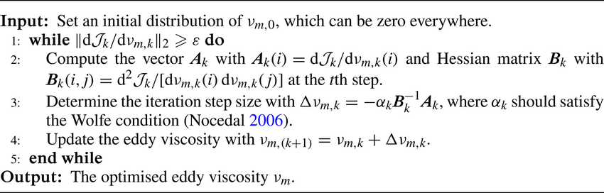
Appendix E. Identification of the energetic structures
To identify the energetic structures in turbulent channel flows, the premultiplied energy amplifications of the optimal harmonic forcing (Hwang & Cossu Reference Hwang and Cossu2010b) predicted by the eLNS $_{MEAN}$ and eLNS
 $_{MOD}$ are investigated here, which is defined by
 \begin{equation} R(\omega;k_x,k_z) = \mathop{{\max}}\limits_{\tilde{\boldsymbol{d}} \ne \boldsymbol{0}} \frac{\left\| \tilde{\boldsymbol{u}} \right\|^2 }{\|\,\tilde{\boldsymbol{f}}\|^2}. \end{equation}
Here,  $R(\omega ;k_x,k_z)$ is equal to the square of the first singular value of the resolvent operator
 ${{\boldsymbol{\mathsf{H}}}}_{\boldsymbol {k}}$. The maximum response amplification at a given spatial scale is then defined by
 \begin{equation} R_{max}(k_x,k_z) = \mathop{\max}\limits_{\omega}R(\omega;k_x,k_z). \end{equation}
Five cases with  $Re_{\tau } = 1000$–
 $20\,000$ are set to test the capability of the eddy-viscosity models in identifying the energetic structures. The Chebyshev-collocation method is used to spatial discretisation in the wall-normal direction. The numbers of collocation points are equal to 400, 600, 800, 800 and 1000 for cases with
 $Re_{\tau }=1000$, 2000, 5000, 10 000 and 20 000, respectively, which are tested to provide converged results. The mean velocity profile is obtained by integrating
 ${\textrm {d}U^+}/{\textrm {d}\eta } = {-Re_{\tau } \eta }/{\nu _{T}^{+}( \eta ) }$, where
 $\nu _{T}^{+} = ( {\nu _{m, MEAN} + \nu })/{\nu }$.
Figure 33 depicts the premultiplied response to optimal stochastic forcing from eLNS $_{MEAN}$ and eLNS
 $_{MOD}$ with
 $k_x = 0$. The results from both models indicate that the dominant structures in outer units with a peak amplification value corresponds to
 $\lambda _z/h \approx 3.5h$. On the other hand, the inner peaks identified by eLNS
 $_{MEAN}$ and eLNS
 $_{MOD}$ exhibit distinct discrepancies. The inner peaks identified by eLNS
 $_{MEAN}$ is around
 $\lambda _z^+ = 80$, which deviate from the DNS results where
 $\lambda _z^+ \approx 125$ (Lee & Moser Reference Lee and Moser2015; Wang et al. Reference Wang, Wang and He2018). Meanwhile, the eLNS
 $_{MOD}$ well identifies the locations of the inner peaks with
 $\lambda _z^+ \approx 125$ for all the tested cases.
Premultiplied response to optimal harmonic forcing with respect to the spanwise wavenumber for  $Re_{\tau } = 1000$–
 $20\,000$ based on eLNS
 $_{MEAN}$ (a,b) and eLNS
 $_{MOD}$ (c,d): (a,c) scaling in outer units; (b,d) scaling in inner units.


 Open access

