1 Introduction
Although there is no formal definition of ‘turbulence’, we may picture turbulence as a tangle of conceptual vortex tubes and sheets (e.g. figure 2.18 in Davidson Reference Davidson2004). These elementary vortical structures consisting of vortex lines evolve under the influence of their self-induced velocity through the Biot–Savart law. The organized vortical structures with candidate tube-like or sheet-like geometries are described as ‘sinews of turbulence’ (Moffatt, Kida & Ohkitani Reference Moffatt, Kida and Ohkitani1994), and they are hypothesized to be related to some statistical features of turbulence at a large Reynolds number (
 $Re$
). In particular, Lundgren (Reference Lundgren1982, Reference Lundgren1993) demonstrated that the energy spectrum with the five-thirds scaling law can be calculated from an ensemble of strained spiral model vortices, which appears to offer some hope of modelling fine-scale turbulence based on a vortex model with specific geometries (see Pullin & Saffman Reference Pullin and Saffman1998).
The vortex tubes and sheets are presumed to be important in turbulence dynamics, but there is a lack of accurate and objective methods to identify these structures in turbulence or highly chaotic flows. In general, three types of visualization methods have been reported to identify vortical structures from three-dimensional direct numerical simulation (DNS) in the literature as follows.
(i) Vorticity vector and vortex line. The early visualizations of vortical structures from DNS of homogeneous isotropic turbulence (HIT) simply plot the vorticity vector field with the vorticity magnitude above a specified threshold (e.g. Kerr Reference Kerr1985; Ruetsch & Maxey Reference Ruetsch and Maxey1991; Vincent & Meneguzzi Reference Vincent and Meneguzzi1991, Reference Vincent and Meneguzzi1994). However, a swarm of vorticity vector arrows with chaotic directions may not well capture the spatial coherence of vortical structures in high-
 $Re$
turbulence. The vortex line, an integral curve of vorticity, is another natural candidate, but it is difficult to objectively select seed points so that vortex lines form coherent structures or have a spatial density proportional to vorticity magnitude (Weißmann, Pinkall & Schröder Reference Weißmann, Pinkall and Schröder2014). Although we can intentionally select the seed points of interest, e.g. the region with large vorticity magnitude (see She, Jackson & Orszag Reference She, Jackson and Orszag1990), a general algorithm of plotting coherent vortex lines in turbulence is still lacking.
(ii) Eulerian vortex-identification criteria. In order to display the vortical structures as smooth surfaces in turbulence, we can use the isosurface of a scalar field related to vorticity. The simplest choice is the vorticity magnitude (e.g. Jimenez et al.
Reference Jimenez, Wray, Saffman and Rogallo1993; Ishihara et al.
Reference Ishihara, Kaneda, Yokokawa, Itakura and Uno2007), which visualizes intermittent vortical structures in very high-
 $Re$
HIT. Furthermore, several vortex-identification criteria based on the Eulerian velocity gradient tensor were proposed to distinguish the highly rotational region or ‘vortex core’ from the large vorticity field in shear flows (e.g. Hunt, Wray & Moin Reference Hunt, Wray and Moin1988; Jeong & Hussain Reference Jeong and Hussain1995; Zhou et al.
Reference Zhou, Adrian, Balachandar and Kendall1999). On the other hand, the isosurfaces of the Eulerian vortex identification criteria cannot accurately display the real vortex tubes and sheets, because they lose the directional information of vorticity and the resultant surfaces can be significantly misaligned with vortex lines. The confusion between the isosurface of these identification criteria and the vortex surface can lead to the misinterpretation of some critical vortex dynamics (see Kida & Takaoka Reference Kida and Takaoka1994; Zhao, Yang & Chen Reference Zhao, Yang and Chen2016a
).
(iii) Vortex surfaces. The vortex tubes and sheets can be generalized as vortex surfaces (or ‘vorticity surfaces’ in some literature). Within the representation of Clebsch (Reference Clebsch1859), Yang & Pullin (Reference Yang and Pullin2010) define the vortex-surface field (VSF) as a smooth scalar field whose isosurfaces are vortex surfaces, and the VSF has been used to construct vortex surfaces in highly symmetric flows (Yang & Pullin Reference Yang and Pullin2010; He & Yang Reference He and Yang2016) and shear flows (Xiong & Yang Reference Xiong and Yang2017). Subsequently, Yang & Pullin (Reference Yang and Pullin2011) develop the two-time method with a dissipative numerical regularization to compute the Lagrangian-like evolution of VSFs in viscous flows, and the evolving VSF has been used to analyse the dynamics of vortex surfaces in transitional wall flows (Zhao, Yang & Chen Reference Zhao, Yang and Chen2016b ; Zhao et al. Reference Zhao, Xiong, Yang and Chen2018), compressible flows (Peng & Yang Reference Peng and Yang2018), reacting flows (Zhou et al. Reference Zhou, You, Xiong, Yang, Thévenin and Chen2019) and magnetohydrodynamic flows (Hao, Xiong & Yang Reference Hao, Xiong and Yang2019). In addition, Chern et al. (Reference Chern, Knöppel, Pinkall and Schröder2017) develop the spherical Clebsch map to visualize vortex lines and surfaces in computer graphics. Although the VSF is applicable to flows with moderately complex vorticity fields, the construction of exact, unique and globally smooth vortex surfaces in general three-dimensional flows and particularly in fully developed turbulence appears to be impossible.
In the present study, we extend the construction of VSFs from simple flow fields with symmetries or dominant vorticity directions, which can significantly facilitate VSF construction, to HIT with very chaotic vortex lines, which is one of the most challenging cases for constructing VSFs. The numerical implementation of constructing the VSF for a given instantaneous vorticity field is to evolve an arbitrary scalar field into an approximate VSF solution by solving a pseudo-transport equation (Yang & Pullin Reference Yang and Pullin2011). This pseudo-transport equation is a first-order convection equation driven by the ‘frozen’ vorticity, which can easily cause numerical oscillation. In particular, some portion of the numerical VSF solution tends to evolve into nearly singular structures owing to the persistent straining motion driven by the chaotic and intermittent vorticity field in fully developed HIT (Pullin & Yang Reference Pullin and Yang2014). In other words, some parts of the accurate VSF solution tend to be non-differentiable in turbulence.
Hence, the major challenge for constructing VSFs in HIT is to balance the accuracy and smoothness of numerical VSF solutions on a finite number of grid points. The total-variation-diminishing (TVD) schemes can partially suppress scalar oscillations (see Hirsch Reference Hirsch1990; Tannehill, Anderson & Pletcher Reference Tannehill, Anderson and Pletcher2012) to ensure the smoothness of VSF solutions, but they suffer the relatively low accuracy, e.g. Goodman & Leveque (Reference Goodman and Leveque1985) proved that any conservative TVD scheme for solving scalar conservation laws in two-dimensional space is at most first-order accurate. An alternative approach is to introduce a penalty function (e.g. Galar et al. Reference Galar, Jurio, Lopez-Molina, Paternain, Sanz and Bustince2013) associated with the scalar gradient to achieve an approximative TVD property by reducing the norm of scalar gradient during VSF calculation.
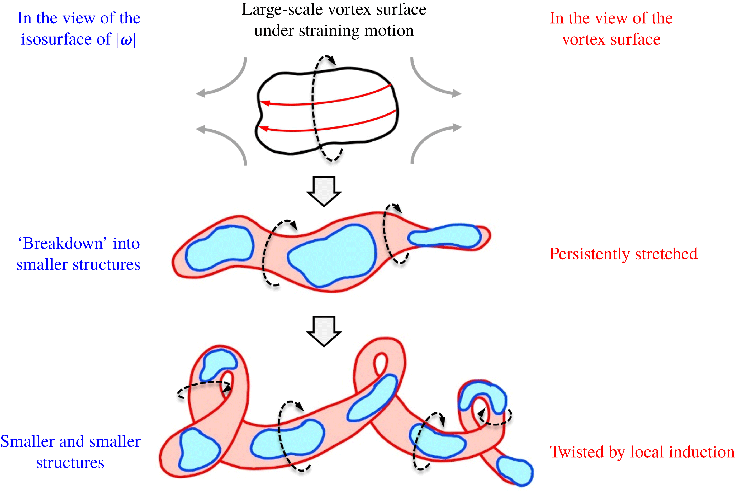
Furthermore, a topic closely related to the identification of vortex surfaces is the physical picture of energy cascade in turbulence (e.g. Goto Reference Goto2008; Wan et al. Reference Wan, Xiao, Meneveau, Eyink and Chen2010; Cardesa, Vela-Martin & Jimenez Reference Cardesa, Vela-Martin and Jimenez2017; Carter & Coletti Reference Carter and Coletti2018). From the hypothesis of Richardson (Reference Richardson1920) and Kolmogorov (Reference Kolmogorov1941b ), three-dimensional HIT is often viewed as composed of different scales with energy transferred from large scales to small scales in a self-similar process, but different structure-identification methods may depict different pathways in this multi-stage process. Using Eulerian vortex-identification methods, the vortical structures are visualized as a cluster of short and broken structures perhaps with fractal features (e.g. Jimenez et al. Reference Jimenez, Wray, Saffman and Rogallo1993; Moisy & Jimenez Reference Moisy and Jimenez2004; Ishihara et al. Reference Ishihara, Kaneda, Yokokawa, Itakura and Uno2007). Based on the Lagrangian view or vorticity equation, some studies speculated that the vortical structures are persistently stretched and twisted (e.g. She, Jackson & Orszag Reference She, Jackson and Orszag1991; Vincent & Meneguzzi Reference Vincent and Meneguzzi1994; Horiuti & Fujisawa Reference Horiuti and Fujisawa2008; Yang, Pullin & Bermejo-Moreno Reference Yang, Pullin and Bermejo-Moreno2010), which is consistent with the formation of the strained spiral vortex model proposed by Lundgren (Reference Lundgren1982). Lundgren & Mansour (Reference Lundgren and Mansour1996) commented that the spirals are commonly seen in experimental visualization but appear to be harder to observe in DNS, so Pullin & Saffman (Reference Pullin and Saffman1998) pointed out that the development of a visualization technique for characterizing vortex tubes remains a considerable challenge.
Therefore, the major objective of the present study is to develop a numerical method to calculate a smooth and relatively accurate VSF solution in an arbitrary flow field with a moderate number of grid points, so that we can obtain the VSF solution to identify the tangle of highly convoluted vortex tubes in HIT. Compared with the existing structure-identification methods, the isosurface of numerical VSF solutions provides the best approximation of vortex surfaces, and the VSF isocontour level can be fixed without the subjective threshold selection in visualization. The morphology of vortex surfaces in decaying HIT is consistent with the equation of vorticity dynamics and can be used to elucidate vortex dynamics in energy cascade. Additionally, the VSF construction at a time instant in HIT can be used as an initial VSF condition for the further calculation of the temporal evolution of VSFs in viscous flows (see Yang & Pullin Reference Yang and Pullin2011).
The outline of this paper is as follows. In § 2, we describe the numerical details of DNS. In § 3, we provide an overview of the theoretical formulation and numerical implementation of the VSF construction. In § 4, we illustrate the identification of twisted vortex tubes in simple Taylor–Green (TG) flows. In § 5, we visualize and characterize the vortex surfaces in decaying HIT. Some conclusions are drawn in § 6.
2 DNS
2.1 Numerical methods
The fluid velocity field
 $\boldsymbol{u}(\boldsymbol{x},t)$
of an incompressible viscous flow is governed by the Navier–Stokes (NS) equations
 $$\begin{eqnarray}\left\{\begin{array}{@{}l@{}}\displaystyle \frac{\unicode[STIX]{x2202}\boldsymbol{u}}{\unicode[STIX]{x2202}t}+(\boldsymbol{u}\boldsymbol{\cdot }\unicode[STIX]{x1D735})\boldsymbol{u}=-\frac{1}{\unicode[STIX]{x1D70C}}\unicode[STIX]{x1D735}p+\unicode[STIX]{x1D708}\unicode[STIX]{x1D6FB}^{2}\boldsymbol{u},\quad \\ \displaystyle \unicode[STIX]{x1D735}\boldsymbol{\cdot }\boldsymbol{u}=0,\quad \end{array}\right.\end{eqnarray}$$
where
 $\boldsymbol{x}$
denotes spatial coordinates,
 $t$
the time,
 $p$
the pressure,
 $\unicode[STIX]{x1D70C}$
the density and
 $\unicode[STIX]{x1D708}$
the kinematic viscosity.
The DNS of decaying HIT is performed to solve (2.1) in a periodic box of side
 $L=2\unicode[STIX]{x03C0}$
using a standard pseudo-spectral method (see Rogallo Reference Rogallo1981; Yang et al.
Reference Yang, Pullin and Bermejo-Moreno2010). The computational domain
 $\unicode[STIX]{x1D6FA}$
is discretized on uniform grid points
 $N^{3}$
. Aliasing errors are removed using the two-thirds truncation method with the maximum wavenumber
 $k_{max}\approx N/3$
. The Fourier coefficient of the velocity is advanced in time using a second-order Adams–Bashforth method, and the time step is chosen to ensure that the Courant–Friedrichs–Lewy (CFL) number is less than
 $0.5$
for numerical stability and accuracy.
The initial velocity
 $\boldsymbol{u}_{0}\equiv \boldsymbol{u}(\boldsymbol{x},t=0)$
for decaying HIT is a random Gaussian field with the initial total energy
 $E_{0}\equiv \int |\boldsymbol{u}_{0}|^{2}/2\,\text{d}\boldsymbol{x}=1$
and a prescribed energy spectrum (e.g. Kraichnan Reference Kraichnan1970; Ishida, Davidson & Kaneda Reference Ishida, Davidson and Kaneda2006)
 $$\begin{eqnarray}E(k,t=0)\sim k^{4}\text{e}^{-2(k/k_{p})^{2}},\end{eqnarray}$$
where
 $k=|\boldsymbol{k}|$
denotes the wavenumber magnitude. The wavenumber
 $k_{p}=4$
where
 $E(k,t=0)$
peaks was selected to ensure that the fully developed HIT field has a broad range of length scales, and it is comparable to the choices of
 $k_{p}$
in previous DNS (e.g. Hosokawa & Yamamoto Reference Hosokawa and Yamamoto1986; Elghobashi & Truesdell Reference Elghobashi and Truesdell1992; Mansour & Wray Reference Mansour and Wray1994).
Additionally, in order to illustrate the identification of twisted vortex tubes, we carry out another DNS of TG flows (Taylor & Green Reference Taylor and Green1937; Brachet et al. Reference Brachet, Meiron, Orszag, Nickel, Morf and Frisch1983) with the initial velocity
 $$\begin{eqnarray}\boldsymbol{u}_{0}=(\sin x\cos y\cos z,-\cos x\sin y\cos z,0)\end{eqnarray}$$
at various Reynolds numbers
 $Re=1/\unicode[STIX]{x1D708}$
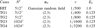
. The initial set-up parameters of the DNS of decaying HIT, as well as the TG flows at four
 $Re$
, are summarized in table 1.
Set-up of DNS cases.

2.2 DNS statistics
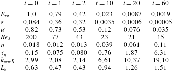
Important statistics in the DNS of decaying HIT at six typical times are summarized in table 2, including the total turbulent kinetic energy
 $E_{tot}=\int E(k)\,\text{d}k$
, mean dissipation rate
 $\unicode[STIX]{x1D700}=2\unicode[STIX]{x1D708}\int k^{2}E(k)\,\text{d}k$
, root-mean-square velocity
 $u^{\prime }=(2E_{tot}/3)^{1/2}$
, Taylor–Reynolds number
 $Re_{\unicode[STIX]{x1D706}}=u^{\prime }\unicode[STIX]{x1D706}_{T}/\unicode[STIX]{x1D708}$
with the Taylor micro-length scale
 $\unicode[STIX]{x1D706}_{T}=(15\unicode[STIX]{x1D708}{u^{\prime }}^{2}/\unicode[STIX]{x1D700})^{1/2}$
, Kolmogorov length scale
 $\unicode[STIX]{x1D702}=(\unicode[STIX]{x1D708}^{3}/\unicode[STIX]{x1D700})^{1/4}$
, Kolmogorov time scale
 $\unicode[STIX]{x1D70F}_{\unicode[STIX]{x1D702}}=(\unicode[STIX]{x1D708}/\unicode[STIX]{x1D700})^{1/2}$
, spatial resolution
 $k_{max}\unicode[STIX]{x1D702}$
and integral length scale
 $L_{e}=\unicode[STIX]{x03C0}/(2{u^{\prime }}^{2})\int E(k)/k\,\text{d}k$
. We remark that the spatial resolution in the present DNS is always greater than two, which satisfies the common criterion
 $k_{max}\unicode[STIX]{x1D702}>1.5$
(Pope Reference Pope2000) for resolving the smallest scales in HIT.
Statistics in the DNS of decaying HIT at six typical times.

From the temporal evolution of
 $E_{tot}$
,
 $\unicode[STIX]{x1D700}$
and
 $E(k)$
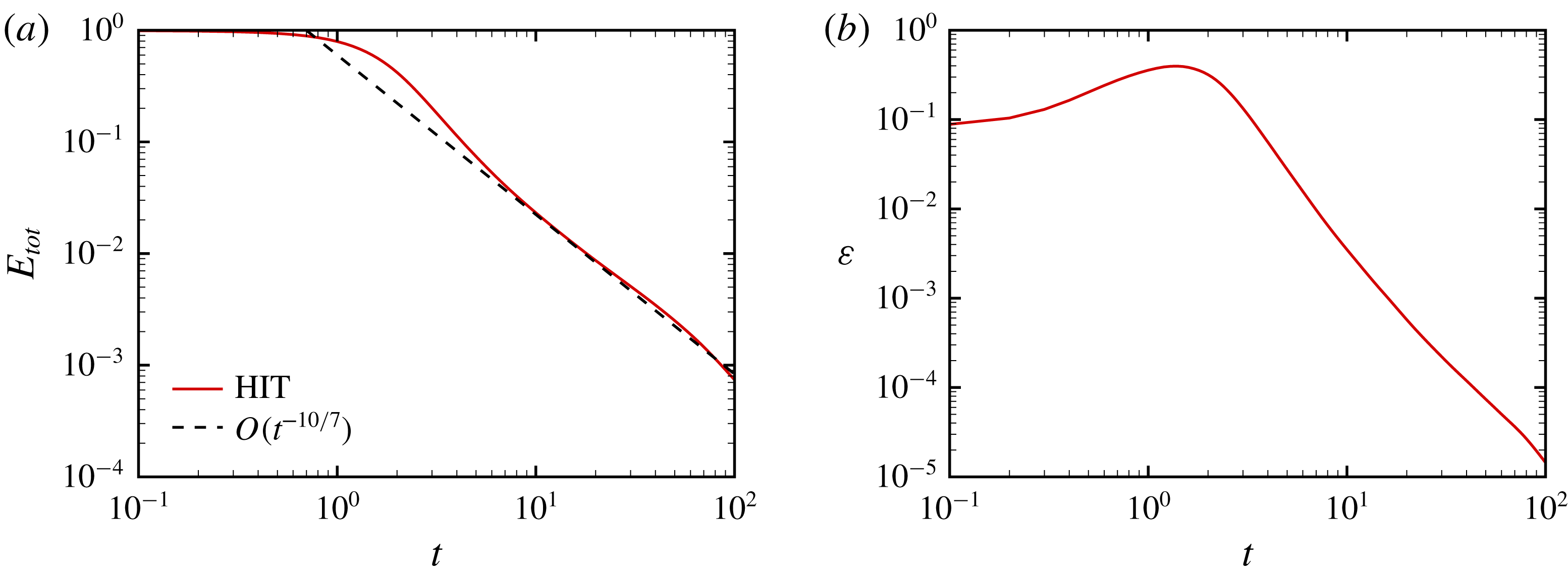
in the DNS of decaying HIT in figures 1(a), 1(b) and 2(a), we generally divide the flow evolution into two stages. In the early stage, the dissipation increases and the flow field evolves from an artificially constructed random field to the fully developed turbulent state. In the later stage, the dissipation decreases and the turbulent flow gradually decays towards a stationary flow. In figure 1(b), the dissipation peaks around
 $t\approx 2$
, implying that the flow field has the maximum total enstrophy with the most intensive vortical structures. In figure 1(a), the total energy decays with the decay law
 $E_{tot}\sim t^{-10/7}$
(Kolmogorov Reference Kolmogorov1941a
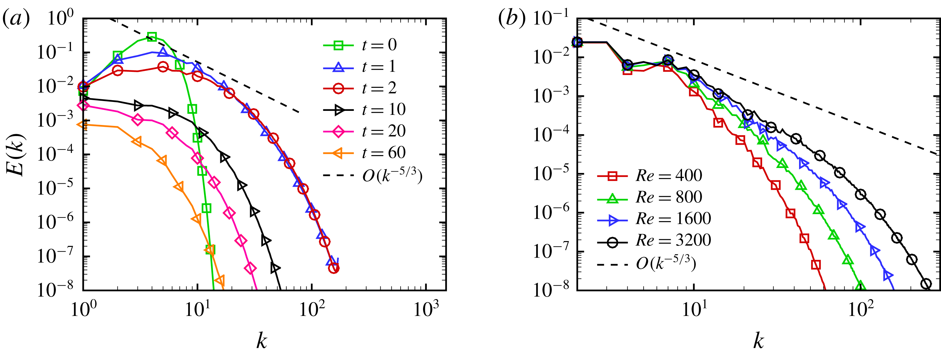
). In figure 2(a), the energy spectrum is gradually broadened in the early stage and has a short inertial region with the five-thirds law
 $E(k)\sim k^{-5/3}$
and a range of length scales in the HIT field at
 $t=2$
. Subsequently the entire spectrum decays in the late stage after
 $t=10$
.
The evolution of TG flows also has two stages similar to the case of decaying HIT (see Brachet et al.
Reference Brachet, Meiron, Orszag, Nickel, Morf and Frisch1983; Yang & Pullin Reference Yang and Pullin2011). Additionally, as
 $Re$
increases, the energy spectrum in TG flows at the two-stage separation point
 $t=7.5$
in figure 2(b) is broadened and approaches the fully developed turbulent state with the five-thirds law.
Evolution of (a) total energy and (b) mean dissipation rate in HIT.

Energy spectra in (a) HIT at different times and (b) TG flows at
 $t=7.5$
.

3 Construction of VSFs
3.1 VSF constraint and pseudo-transport equation
The VSF
 $\unicode[STIX]{x1D719}_{v}$
is defined as a globally smooth scalar field whose isosurface is a vortex surface consisting of vortex lines. The constraint of the VSF (Yang & Pullin Reference Yang and Pullin2010) is
 $$\begin{eqnarray}{\mathcal{C}}_{v}\equiv \unicode[STIX]{x1D74E}\boldsymbol{\cdot }\unicode[STIX]{x1D735}\unicode[STIX]{x1D719}_{v}=0,\end{eqnarray}$$
where
 $\unicode[STIX]{x1D74E}\equiv \unicode[STIX]{x1D735}\times \boldsymbol{u}$
is the vorticity. The construction of VSF is equivalent to finding a solution of
 $\unicode[STIX]{x1D719}_{v}$
satisfying (3.1) for a given, instantaneous
 $\unicode[STIX]{x1D74E}$
. For a vorticity field with vanishing helicity density
 $h\equiv \boldsymbol{u}\boldsymbol{\cdot }\unicode[STIX]{x1D74E}=0$
, we can obtain exact VSF solutions from (3.1) (He & Yang Reference He and Yang2016). Nonetheless, for a general vorticity field with
 $h\neq 0$
, the non-trivial analytic solution of (3.1) may not exist, so we have to seek an approximate solution of (3.1) using numerical methods.
Based on the definition of VSF, the deviation of an approximate VSF solution
 $\unicode[STIX]{x1D719}_{v}$
from an exact VSF is defined as the cosine of the angle between
 $\unicode[STIX]{x1D74E}$
and
 $\unicode[STIX]{x1D735}\unicode[STIX]{x1D719}_{v}$
as (Yang & Pullin Reference Yang and Pullin2010)
 $$\begin{eqnarray}\unicode[STIX]{x1D706}_{\unicode[STIX]{x1D714}}\equiv \frac{\unicode[STIX]{x1D74E}\boldsymbol{\cdot }\unicode[STIX]{x1D735}\unicode[STIX]{x1D719}_{v}}{|\unicode[STIX]{x1D74E}||\unicode[STIX]{x1D735}\unicode[STIX]{x1D719}_{v}|}.\end{eqnarray}$$
For a given instantaneous vorticity field
 $\unicode[STIX]{x1D74E}$
, the goal of constructing an approximate VSF solution is to minimize the volume-averaged VSF deviation
 $\langle |\unicode[STIX]{x1D706}_{\unicode[STIX]{x1D714}}|\rangle$
by varying
 $\unicode[STIX]{x1D719}_{v}$
.
To obtain an approximate VSF solution, Yang & Pullin (Reference Yang and Pullin2011) developed the pseudo-transport equation
 $$\begin{eqnarray}\frac{\unicode[STIX]{x2202}\unicode[STIX]{x1D719}_{v}}{\unicode[STIX]{x2202}\unicode[STIX]{x1D70F}}+\unicode[STIX]{x1D74E}\boldsymbol{\cdot }\unicode[STIX]{x1D735}\unicode[STIX]{x1D719}_{v}=0,\quad \boldsymbol{x}\in \unicode[STIX]{x1D6FA},\quad 0<\unicode[STIX]{x1D70F}\leqslant T_{\unicode[STIX]{x1D70F}}\end{eqnarray}$$
driven by the given ‘frozen’ vorticity, where
 $T_{\unicode[STIX]{x1D70F}}$
denotes the largest pseudo-time in the VSF calculation. The initial condition
 $\unicode[STIX]{x1D719}_{v0}\equiv \unicode[STIX]{x1D719}_{v}(\boldsymbol{x},\unicode[STIX]{x1D70F}=0)$
of (3.3) can be an arbitrary scalar field with large
 $\langle |\unicode[STIX]{x1D706}_{\unicode[STIX]{x1D714}}|\rangle$
. Although the exact VSF solution is not unique (see Yang & Pullin Reference Yang and Pullin2010), we found that the statistical geometry of converged VSF solutions is insensitive to the choice of
 $\unicode[STIX]{x1D719}_{v0}$
if the given vorticity field is chaotic (see Xiong & Yang Reference Xiong and Yang2017), e.g. in turbulence. The sensitivity of the VSF solution to initial conditions is further discussed in appendix A. Moreover, the boundary conditions for (3.3) should be treated carefully except for the periodic boundary condition that can be naturally applied (see Xiong & Yang Reference Xiong and Yang2017).
3.2 Numerical construction of VSFs with the local optimization
Although the VSF deviation of the solution of (3.3) can be converged at large pseudo-time
 $T_{\unicode[STIX]{x1D70F}}$
, the converged solution tends to have nearly singular structures with a very large scalar gradient owing to the persistent straining of
 $\unicode[STIX]{x1D719}_{v}$
driven by the frozen vorticity in turbulence or highly chaotic flows (see Pullin & Yang Reference Pullin and Yang2014). This dilemma hinders the effective VSF construction and visualization in complex flow fields.
Thus we propose a new hybrid constraint
 $$\begin{eqnarray}{\mathcal{C}}_{h}=(1-\unicode[STIX]{x1D701})|\unicode[STIX]{x1D74E}\boldsymbol{\cdot }\unicode[STIX]{x1D735}\unicode[STIX]{x1D719}_{v}|^{2}+\unicode[STIX]{x1D701}|\unicode[STIX]{x1D735}\unicode[STIX]{x1D719}_{v}|^{2}\end{eqnarray}$$
to balance the small VSF deviation with the desired smoothness of VSF solutions, where
 $\unicode[STIX]{x1D701}$
is a weighting factor to characterize the preference for the minimization of
 $|{\mathcal{C}}_{v}|$
or
 $|\unicode[STIX]{x1D735}\unicode[STIX]{x1D719}_{v}|$
. The construction of a non-trivial normalized VSF solution is then equivalent to an optimization problem as
 $$\begin{eqnarray}\min {\mathcal{C}}_{h},\quad \text{s.t.}\langle \unicode[STIX]{x1D719}_{v}\rangle =0\quad \text{and}\quad \text{Var}(\unicode[STIX]{x1D719}_{v})=1,\end{eqnarray}$$
where
 $\text{Var}(f)\equiv \langle (f-\langle f\rangle )^{2}\rangle$
denotes the variance of an arbitrary function
 $f$
in a volume.
With this key improvement, each computational step in the implementation of VSF construction is divided into two sub-steps: (i) solving the pseudo-transport equation (3.3); (ii) applying the local optimization (3.5). First, a temporary VSF
 $\unicode[STIX]{x1D719}_{v}^{\ast }$
is evolved as (3.3) in pseudo-time, where
 $\unicode[STIX]{x1D719}_{v}^{\ast }$
is advanced in
 $\unicode[STIX]{x1D70F}$
using the third-order TVD Runge–Kutta method, and the convection term is approximated by the fifth-order weighted essentially non-oscillatory (WENO) scheme (Jiang & Shu Reference Jiang and Shu1996). The pseudo-time step should be small enough to ensure that the CFL number based on vorticity is less than 0.5 for numerical stability.
Subsequently, we minimize
 ${\mathcal{C}}_{h}$
to obtain a local optimized solution
 $\tilde{\unicode[STIX]{x1D719}}_{v}$
, where the weighting factor in (3.4) is chosen as
 $$\begin{eqnarray}\unicode[STIX]{x1D701}(\unicode[STIX]{x1D70F})=(1-\unicode[STIX]{x1D70F}/T_{\unicode[STIX]{x1D70F}})^{2}.\end{eqnarray}$$
In other words, we prefer smooth VSF solutions for small
 $\unicode[STIX]{x1D70F}$
and accurate solutions for large
 $\unicode[STIX]{x1D70F}$
. It is noted that the specific form of (3.6) is ad hoc based on both the accuracy and smoothness of VSF solutions in numerical experiments. In general, if
 $\unicode[STIX]{x1D701}=1$
or
 $\unicode[STIX]{x1D701}$
is closer to unity than (3.6),
 $\langle |\unicode[STIX]{x1D706}_{\unicode[STIX]{x1D714}}|\rangle$
and
 $\sqrt{\langle |\unicode[STIX]{x1D735}\unicode[STIX]{x1D719}_{v}|^{2}\rangle }$
tend to slightly increase and decrease at large
 $\unicode[STIX]{x1D70F}$
, respectively, but geometries of corresponding VSF isosurfaces are almost identical. Furthermore, appendix B provides a two-dimensional example to illustrate the effect of the local optimization and the choice of
 $\unicode[STIX]{x1D701}$
on VSF calculation.
The numerical algorithm of minimizing the hybrid constraint
 ${\mathcal{C}}_{h}$
using the variational method is described in detail below. The minimization of
 ${\mathcal{C}}_{h}$
in (3.4) by varying
 $\unicode[STIX]{x1D719}_{v}^{\ast }$
is equivalent to a local optimization problem satisfying
 $$\begin{eqnarray}\frac{\unicode[STIX]{x2202}\Vert {\mathcal{C}}_{h}(\unicode[STIX]{x1D719}_{v}^{\ast }(\boldsymbol{a}),\boldsymbol{x})\Vert _{\unicode[STIX]{x1D6FF}\unicode[STIX]{x1D6FA}}}{\unicode[STIX]{x2202}\unicode[STIX]{x1D719}_{v}^{\ast }(\boldsymbol{a})}=0\quad \text{and}\quad \frac{\unicode[STIX]{x2202}^{2}\Vert {\mathcal{C}}_{h}(\unicode[STIX]{x1D719}_{v}^{\ast }(\boldsymbol{a}),\boldsymbol{x})\Vert _{\unicode[STIX]{x1D6FF}\unicode[STIX]{x1D6FA}}}{\unicode[STIX]{x2202}\unicode[STIX]{x1D719}_{v}^{\ast }(\boldsymbol{a})^{2}}>0.\end{eqnarray}$$
Here,
 $\boldsymbol{a}$
denotes the coordinates at which
 $\unicode[STIX]{x1D719}_{v}^{\ast }$
is varied in the optimization, and
 $\Vert f\Vert _{\unicode[STIX]{x1D6FF}\unicode[STIX]{x1D6FA}}\equiv \int _{\unicode[STIX]{x1D6FF}\unicode[STIX]{x1D6FA}}|f|\,\text{d}\boldsymbol{x}$
denotes the
 $L_{1}$
norm of a function
 $f$
over a finite subdomain
 $\unicode[STIX]{x1D6FF}\unicode[STIX]{x1D6FA}$
containing
 $\boldsymbol{a}$
.
The temporary scalar field
 $\unicode[STIX]{x1D719}_{v}^{\ast }$
is discretized on uniform grid points
 $N_{\unicode[STIX]{x1D719}}^{3}$
in computational domain
 $\unicode[STIX]{x1D6FA}$
. Coordinates for the uniform grids are
 $\boldsymbol{x}_{\boldsymbol{i}}\equiv (x_{i},y_{j},z_{k})=(i\unicode[STIX]{x0394}x,j\unicode[STIX]{x0394}x,k\unicode[STIX]{x0394}x)$
with grid spacing
 $\unicode[STIX]{x0394}x=2\unicode[STIX]{x03C0}/N_{\unicode[STIX]{x1D719}}$
, which can be expressed as a point set
 $$\begin{eqnarray}G=\{\boldsymbol{x}_{\boldsymbol{i}}\mid i,j,k\in \{0,1,\ldots ,N_{\unicode[STIX]{x1D719}}-1\}\}.\end{eqnarray}$$
In the local optimization,
 $\unicode[STIX]{x1D719}_{v}^{\ast }$
is varied on coarse staggered grids. Coordinates for the staggered grids are
 $\boldsymbol{a}_{\boldsymbol{m}}\equiv (a_{m},b_{n},c_{l})=(m\unicode[STIX]{x0394}x,n\unicode[STIX]{x0394}x,l\unicode[STIX]{x0394}x)$
. The
 $N_{\unicode[STIX]{x1D719}}^{3}/(n_{s}+1)$
variational points are selected as a subset of
 $G$
as
 $$\begin{eqnarray}G^{\prime }=\{\boldsymbol{a}_{\boldsymbol{ m}}\mid m,n,l\in \{0,1,\ldots ,N_{\unicode[STIX]{x1D719}}-1\}\text{ and }m+n+l\equiv 0~(\text{mod}~n_{s}+1)\},\end{eqnarray}$$
where
 $n_{s}$
is the order of the finite difference scheme utilized for evaluating
 ${\mathcal{C}}_{h}$
, and satisfies
 $N_{\unicode[STIX]{x1D719}}\equiv 0~(\text{mod}~n_{s}+1)$
. The staggered grids and a specific finite difference scheme define staggered overlapping subdomains
 $\unicode[STIX]{x1D6FF}\unicode[STIX]{x1D6FA}_{\boldsymbol{m}}$
, so that the variation of
 $\unicode[STIX]{x1D719}_{v}^{\ast }$
at
 $\boldsymbol{a}_{\boldsymbol{m}}$
only influences
 ${\mathcal{C}}_{h}$
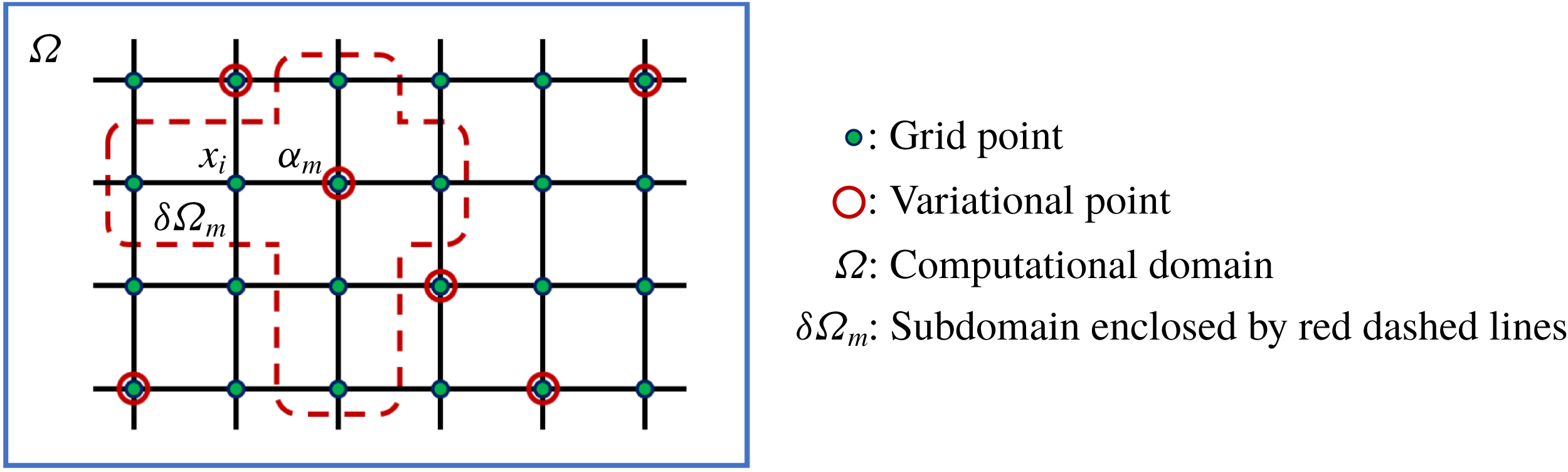
in each subdomain. In the schematic diagram in figure 3, each
 $\unicode[STIX]{x1D6FF}\unicode[STIX]{x1D6FA}_{\boldsymbol{m}}$
is enclosed by red dashed lines, and it only has one variational point at
 $\boldsymbol{a}_{\boldsymbol{m}}$
marked by the open circle to avoid the interference among the variations of
 $\unicode[STIX]{x1D719}_{v}^{\ast }$
at multiple points in the subdomain.
The discretized
 $L_{1}$
norm of
 ${\mathcal{C}}_{h}(\unicode[STIX]{x1D719}_{v}^{\ast }(\boldsymbol{a}_{\boldsymbol{m}}),\boldsymbol{x}_{\boldsymbol{i}})$
over each
 $\unicode[STIX]{x1D6FF}\unicode[STIX]{x1D6FA}_{\boldsymbol{m}}$
is minimized by varying
 $\unicode[STIX]{x1D719}_{v}^{\ast }(\boldsymbol{a}_{\boldsymbol{m}})$
. A third-order difference scheme with
 $n_{s}=3$
is applied to compute the gradient of
 $\unicode[STIX]{x1D719}_{v}^{\ast }(\boldsymbol{x}_{\boldsymbol{i}})$
in
 ${\mathcal{C}}_{h}(\unicode[STIX]{x1D719}_{v}^{\ast }(\boldsymbol{a}_{\boldsymbol{m}}),\boldsymbol{x}_{\boldsymbol{i}})$
, e.g. the partial derivative respect to
 $x$
at specific
 $\boldsymbol{x}_{\boldsymbol{i}}$
on the left of
 $\boldsymbol{a}_{\boldsymbol{m}}=\boldsymbol{x}_{\boldsymbol{i}}+\unicode[STIX]{x0394}\boldsymbol{x}$
(see figure 3) with
 $\unicode[STIX]{x0394}\boldsymbol{x}=(\unicode[STIX]{x0394}x,0,0)$
is discretized as
 $$\begin{eqnarray}\frac{\unicode[STIX]{x2202}\unicode[STIX]{x1D719}_{v}^{\ast }(\boldsymbol{x}_{\boldsymbol{i}})}{\unicode[STIX]{x2202}x}=\frac{1}{\unicode[STIX]{x0394}x}\unicode[STIX]{x1D719}_{v}^{\ast }(\boldsymbol{a}_{\boldsymbol{ m}})-\frac{1}{6\unicode[STIX]{x0394}x}[2\unicode[STIX]{x1D719}_{v}^{\ast }(\boldsymbol{x}_{\boldsymbol{ i}}-\unicode[STIX]{x0394}\boldsymbol{x})+3\unicode[STIX]{x1D719}_{v}^{\ast }(\boldsymbol{x}_{\boldsymbol{ i}})+\unicode[STIX]{x1D719}_{v}^{\ast }(\boldsymbol{x}_{\boldsymbol{ i}}+2\unicode[STIX]{x0394}\boldsymbol{x})].\end{eqnarray}$$
The partial derivatives respect to
 $y$
and
 $z$
have a similar form to (3.10). Substituting all the discretized partial derivatives in three directions into (3.4) yields the discretized hybrid constraint in a polynomial form as
 $$\begin{eqnarray}{\mathcal{C}}_{h}(\unicode[STIX]{x1D719}_{v}^{\ast }(\boldsymbol{a}_{\boldsymbol{ m}}),\boldsymbol{x}_{\boldsymbol{i}})=\unicode[STIX]{x1D709}_{2}(\boldsymbol{x}_{\boldsymbol{i}},\boldsymbol{a}_{\boldsymbol{m}})\unicode[STIX]{x1D719}_{v}^{\ast }(\boldsymbol{a}_{\boldsymbol{ m}})^{2}+\unicode[STIX]{x1D709}_{1}(\boldsymbol{x}_{\boldsymbol{i}},\boldsymbol{a}_{\boldsymbol{m}})\unicode[STIX]{x1D719}_{v}^{\ast }(\boldsymbol{a}_{\boldsymbol{ m}})+\unicode[STIX]{x1D709}_{0}(\boldsymbol{x}_{\boldsymbol{i}},\boldsymbol{a}_{\boldsymbol{m}}),\end{eqnarray}$$
where
 $\unicode[STIX]{x1D709}_{0}$
,
 $\unicode[STIX]{x1D709}_{1}$
and
 $\unicode[STIX]{x1D709}_{2}$
are obtained by collecting finite difference coefficients in the discretized partial derivatives such as (3.10). After the discretization, (3.7) is re-expressed as
 $$\begin{eqnarray}\frac{\unicode[STIX]{x2202}}{\unicode[STIX]{x2202}\unicode[STIX]{x1D719}_{v}^{\ast }(\boldsymbol{a}_{\boldsymbol{m}})}\left[\mathop{\sum }_{\boldsymbol{x}_{\boldsymbol{i}}\in \unicode[STIX]{x1D6FF}\unicode[STIX]{x1D6FA}_{\boldsymbol{m}}}{\mathcal{C}}_{h}(\unicode[STIX]{x1D719}_{v}^{\ast }(\boldsymbol{a}_{\boldsymbol{ m}}),\boldsymbol{x}_{\boldsymbol{i}})\right]=\mathop{\sum }_{\boldsymbol{x}_{\boldsymbol{i}}\in \unicode[STIX]{x1D6FF}\unicode[STIX]{x1D6FA}_{\boldsymbol{m}}}[2\unicode[STIX]{x1D709}_{2}(\boldsymbol{x}_{\boldsymbol{i}},\boldsymbol{a}_{\boldsymbol{m}})\unicode[STIX]{x1D719}_{v}^{\ast }(\boldsymbol{a}_{\boldsymbol{ m}})+\unicode[STIX]{x1D709}_{1}(\boldsymbol{x}_{\boldsymbol{i}},\boldsymbol{a}_{\boldsymbol{m}})]=0,\end{eqnarray}$$
and the corresponding second partial derivative only containing squared terms must be positive. Thus scalar values at all the variational points
 $\boldsymbol{a}_{\boldsymbol{i}}$
are optimized as
 $$\begin{eqnarray}\unicode[STIX]{x1D719}_{v}^{\prime }(\boldsymbol{a}_{\boldsymbol{ m}})=-\frac{1}{2}\mathop{\sum }_{\boldsymbol{x}_{\boldsymbol{i}}\in \unicode[STIX]{x1D6FF}\unicode[STIX]{x1D6FA}_{\boldsymbol{m}}}\unicode[STIX]{x1D709}_{1}(\boldsymbol{x}_{\boldsymbol{i}},\boldsymbol{a}_{\boldsymbol{m}})\bigg/\mathop{\sum }_{\boldsymbol{x}_{\boldsymbol{i}}\in \unicode[STIX]{x1D6FF}\unicode[STIX]{x1D6FA}_{\boldsymbol{m}}}\unicode[STIX]{x1D709}_{2}(\boldsymbol{x}_{\boldsymbol{i}},\boldsymbol{a}_{\boldsymbol{m}})\end{eqnarray}$$
to minimize the local hybrid constraint.
Schematic diagram for the subdivision of the computational domain.

Finally, the VSF solution in the local optimization sub-step is updated as
 $$\begin{eqnarray}\tilde{\unicode[STIX]{x1D719}}_{v}(\boldsymbol{x}_{\boldsymbol{i}})=\left\{\begin{array}{@{}ll@{}}\unicode[STIX]{x1D719}_{v}^{\prime }(\boldsymbol{x}_{\boldsymbol{i}}),\quad & \text{if }\boldsymbol{x}_{\boldsymbol{i}}\in G^{\prime },\\ \unicode[STIX]{x1D719}_{v}^{\ast }(\boldsymbol{x}_{\boldsymbol{i}}),\quad & \text{if }\boldsymbol{x}_{\boldsymbol{i}}\in G\setminus G^{\prime }.\end{array}\right.\end{eqnarray}$$
Then the VSF solution is normalized to zero mean and unity variance as
 $$\begin{eqnarray}\unicode[STIX]{x1D719}_{v}=\frac{\tilde{\unicode[STIX]{x1D719}}_{v}-\langle \tilde{\unicode[STIX]{x1D719}}_{v}\rangle }{\sqrt{\text{Var}(\tilde{\unicode[STIX]{x1D719}}_{v})}}.\end{eqnarray}$$
3.3 Assessment of VSF construction
We construct VSFs from instantaneous vorticity fields in DNS of decaying HIT at six typical times listed in table 2. The number of grid points
 $N_{\unicode[STIX]{x1D719}}^{3}$
for the VSF, as listed in table 3, can be larger than required
 $N^{3}$
for DNS, and
 $\unicode[STIX]{x1D74E}$
from DNS is interpolated onto the finer VSF grids by the cubic spline interpolation for further VSF construction. In general, required
 $N_{\unicode[STIX]{x1D719}}^{3}$
increases with decreasing the tolerance of
 $\langle |\unicode[STIX]{x1D706}_{\unicode[STIX]{x1D714}}|\rangle$
or increasing the complexity of vorticity.
The number of scalar grid points and CPU hours in the construction of VSFs in decaying HIT at six typical times.

The initial condition
 $\unicode[STIX]{x1D719}_{v0}$
is a spatial delta-correlated field in which the scalar value at each point is generated independently as a random number satisfying the uniform distribution from 0 to 1. Although a tailored smooth
 $\unicode[STIX]{x1D719}_{v0}$
should achieve faster convergence in VSF construction, the present choice avoids the subjective selection of
 $\unicode[STIX]{x1D719}_{v0}$
.
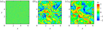
Figure 4 displays the plane cuts of VSF solution contours at three pseudo-times during VSF construction for the HIT field at
 $t=20$
. In the pseudo-evolution, the scalar field evolves from a very noisy initial random field through a fine-scale scalar field at
 $\unicode[STIX]{x1D70F}/T_{v}=1$
to a relatively smooth field at
 $\unicode[STIX]{x1D70F}/T_{v}=4$
when the VSF solution has been nearly converged. Here,
 $T_{v}\equiv L_{\unicode[STIX]{x1D6FA}}/\langle |\unicode[STIX]{x1D74E}|\rangle$
is the characteristic pseudo-time scale (Xiong & Yang Reference Xiong and Yang2017), where the characteristic length scale of the computational domain
 $L_{\unicode[STIX]{x1D6FA}}=2\sqrt{3}\unicode[STIX]{x03C0}$
is the diagonal length of the DNS cube.
Plane cuts of the contour of VSF solutions at three pseudo-times during the VSF construction for HIT at
 $t=20$
. (a)
 $\unicode[STIX]{x1D70F}/T_{v}=0$
; (b)
 $\unicode[STIX]{x1D70F}/T_{v}=1$
; (c)
 $\unicode[STIX]{x1D70F}/T_{v}=4$
.

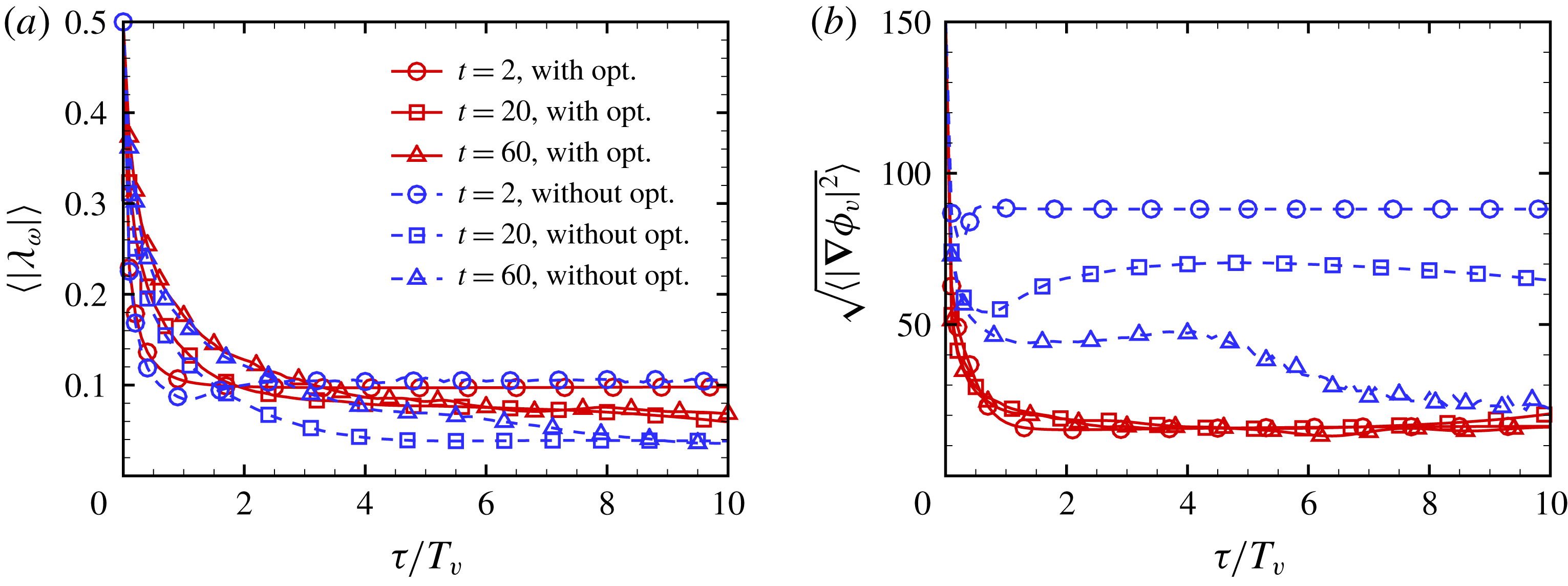
We compare the convergence and smoothness of VSF solutions with and without local optimization. In the VSF construction for instantaneous
 $\unicode[STIX]{x1D74E}$
of decaying HIT at
 $t=2$
, 20 and 60 with
 $N_{\unicode[STIX]{x1D719}}=512$
, pseudo-evolutions of
 $\langle |\unicode[STIX]{x1D706}_{\unicode[STIX]{x1D714}}|\rangle$
and
 $\langle |\unicode[STIX]{x1D735}\unicode[STIX]{x1D719}_{v}|^{2}\rangle$
in normalized pseudo-time
 $\unicode[STIX]{x1D70F}/T_{v}$
are shown in figures 5(a) and 5(b), respectively. In general,
 $\langle |\unicode[STIX]{x1D706}_{\unicode[STIX]{x1D714}}|\rangle$
and
 $\langle |\unicode[STIX]{x1D735}\unicode[STIX]{x1D719}_{v}|^{2}\rangle$
of VSF solutions have converged before
 $\unicode[STIX]{x1D70F}/T_{v}=10$
, so we set
 $T_{\unicode[STIX]{x1D70F}}=10T_{v}$
. Additionally,
 $\langle |\unicode[STIX]{x1D735}\unicode[STIX]{x1D719}_{v}|^{2}\rangle$
without local optimization becomes larger at higher
 $Re_{\unicode[STIX]{x1D706}}$
. By contrast, the pseudo-transport with local optimization significantly reduces the scalar gradient to ensure both satisfactory VSF deviation
 $\langle |\unicode[STIX]{x1D706}_{\unicode[STIX]{x1D714}}|\rangle \leqslant 10\,\%$
and smoothness of VSF solutions, although the optimization strategy of
 $\unicode[STIX]{x1D701}(\unicode[STIX]{x1D70F})$
in (3.6) slightly sacrifices the convergence rate of VSF solutions for small pseudo-times.
The pseudo-evolution of (a)
 $\langle |\unicode[STIX]{x1D706}_{\unicode[STIX]{x1D714}}|\rangle$
and (b)
 $\sqrt{\langle |\unicode[STIX]{x1D735}\unicode[STIX]{x1D719}_{v}|^{2}\rangle }$
in decaying HIT at
 $t=2$
, 20 and 60 with
 $N_{\unicode[STIX]{x1D719}}=512$
and with or without local optimization.

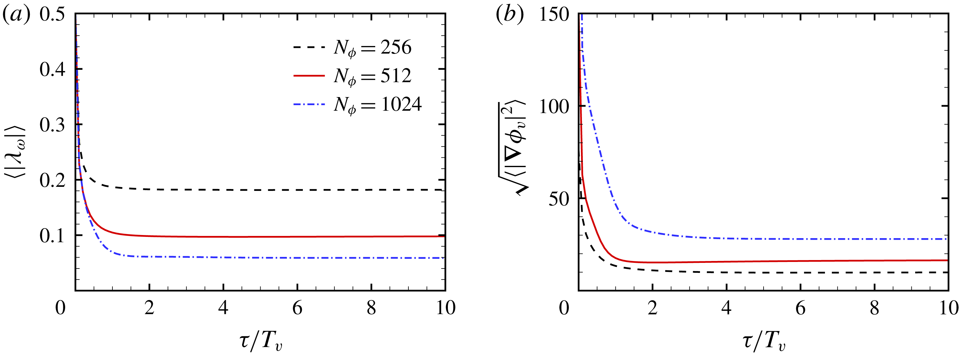
The averaged VSF deviation can be further reduced by increasing the grid resolution for VSF (see Yang & Pullin Reference Yang and Pullin2011). Taking the VSF construction for the most fluctuating HIT field at
 $t=2$
for example,
 $\langle |\unicode[STIX]{x1D706}_{\unicode[STIX]{x1D714}}|\rangle$
is reduced from
 $18\,\%$
with
 $N_{\unicode[STIX]{x1D719}}^{3}=256^{3}$
to
 $6\,\%$
with
 $N_{\unicode[STIX]{x1D719}}^{3}=1024^{3}$
in figure 6(a), and
 $\langle |\unicode[STIX]{x1D706}_{\unicode[STIX]{x1D714}}|\rangle$
for converged numerical VSF solutions is proportional to
 $N_{\unicode[STIX]{x1D719}}^{-0.8}$
. At the meantime,
 $\langle |\unicode[STIX]{x1D735}\unicode[STIX]{x1D719}_{v}|^{2}\rangle$
is increased from
 $10$
with
 $N_{\unicode[STIX]{x1D719}}^{3}=256^{3}$
to
 $28$
with
 $N_{\unicode[STIX]{x1D719}}^{3}=1024^{3}$
in figure 6(b), indicating that the high-resolution VSF solution reveals finer-scale structures of vortex surfaces.
The pseudo-evolution of (a)
 $\langle |\unicode[STIX]{x1D706}_{\unicode[STIX]{x1D714}}|\rangle$
and (b)
 $\sqrt{\langle |\unicode[STIX]{x1D735}\unicode[STIX]{x1D719}_{v}|^{2}\rangle }$
in decaying HIT at
 $t=2$
on different VSF grids with local optimization.

We remark that the VSF construction is computationally expansive, which needs to be improved in future work. The computational time depends on the number of VSF grid points, the tolerance of
 $\langle |\unicode[STIX]{x1D706}_{\unicode[STIX]{x1D714}}|\rangle$
and the complexity of vorticity (see Xiong & Yang Reference Xiong and Yang2017). Typical CPU hours for constructing VSFs in decaying HIT are summarized in table 3.
4 Identification of twisted vortex tubes in TG flows
Before studying the convoluted vortex surfaces in HIT, we first demonstrate the capability of the VSF for identifying relatively isolated vortex tubes in TG flows. As shown in figure 2, the high-
 $Re$
TG flow at the late stage has a similar spectrum as that in HIT, thus the vortex surfaces identified in high-
 $Re$
TG flows can represent some geometrical features in real turbulence.
The former VSF study of TG flows at moderate
 $Re$
in Yang & Pullin (Reference Yang and Pullin2011) suggests that, based on evolutionary geometry and topology of vortex surfaces, the entire VSF evolution can be divided into three stages: (i) vortex flattening; (ii) vortex reconnection during transition; (iii) rolling-up, stretching and twisting of vortex tubes. Furthermore, Yang & Pullin (Reference Yang and Pullin2011) showed that the vortex surfaces of TG flows with
 $Re=400$
and 800 at
 $t=7.5$
in the late stage appear to have the same topology, but the tubes with large
 $Re$
are more twisted than those with small
 $Re$
. The helical vortex tubes (e.g. Ricca Reference Ricca1994; Fukumoto & Okuluv Reference Fukumoto and Okuluv2005) in high-
 $Re$
flows can generate more intense small-scale velocity fields than those in low-
 $Re$
flows.
In the present study, we construct the VSF in TG flows at a range of
 $Re$
from 400 to 3200 by solving the pseudo-transport equation (3.3). Since the velocity–vorticity field has mirror and rotational symmetries in TG flows (Brachet et al.
Reference Brachet, Meiron, Orszag, Nickel, Morf and Frisch1983) which can significantly facilitate the VSF construction (Yang & Pullin Reference Yang and Pullin2010), the boundary-constraint method (Xiong & Yang Reference Xiong and Yang2017) is used to construct VSFs without the sub-step of local optimization (3.5). The VSF for the initial TG field (Yang & Pullin Reference Yang and Pullin2011)
 $\unicode[STIX]{x1D719}_{v0}=(\cos 2x-\cos 2y)\cos z/2$
is used as the initial condition of (3.3). The VSF within
 $[0,\unicode[STIX]{x03C0}/2]\times [0,\unicode[STIX]{x03C0}/2]\times [\unicode[STIX]{x03C0}/2,\unicode[STIX]{x03C0}]$
is calculated on uniform grid points
 $N_{\unicode[STIX]{x1D719}}^{3}$
with
 $N_{\unicode[STIX]{x1D719}}=N/4+1$
in TG flows with different
 $Re$
at
 $t=7.5$
. After the pseudo-evolution from
 $\unicode[STIX]{x1D70F}=0$
to
 $\unicode[STIX]{x1D70F}/T_{v}=2$
, we achieved very accurate VSF solutions as the VSF deviations converge to a level less than
 $4\,\%$
(not shown).
Isosurfaces of
 $\unicode[STIX]{x1D719}_{v}$
and
 $|\unicode[STIX]{x1D74E}|$
in TG flows with different
 $Re$
at
 $t=7.5$
. Some vortex lines are integrated on the isosurfaces of
 $\unicode[STIX]{x1D719}_{v}$
. The vortex lines and the isosurfaces of
 $|\unicode[STIX]{x1D74E}|$
are colour coded by
 $|\unicode[STIX]{x1D74E}|$
. (a)
 $\hat{\unicode[STIX]{x1D719}}_{v}=0.5$
and (b)
 $|\unicode[STIX]{x1D74E}|=7.0$
at
 $Re=400$
; (c)
 $\hat{\unicode[STIX]{x1D719}}_{v}=0.5$
and (d)
 $|\unicode[STIX]{x1D74E}|=10.0$
at
 $Re=800$
; (e)
 $\hat{\unicode[STIX]{x1D719}}_{v}=0.5$
and (f)
 $|\unicode[STIX]{x1D74E}|=15.0$
at
 $Re=1600$
; (g)
 $\hat{\unicode[STIX]{x1D719}}_{v}=0.5$
and (h)
 $|\unicode[STIX]{x1D74E}|=27.0$
at
 $Re=3200$
.

At the late stage of TG flows at
 $t=7.5$
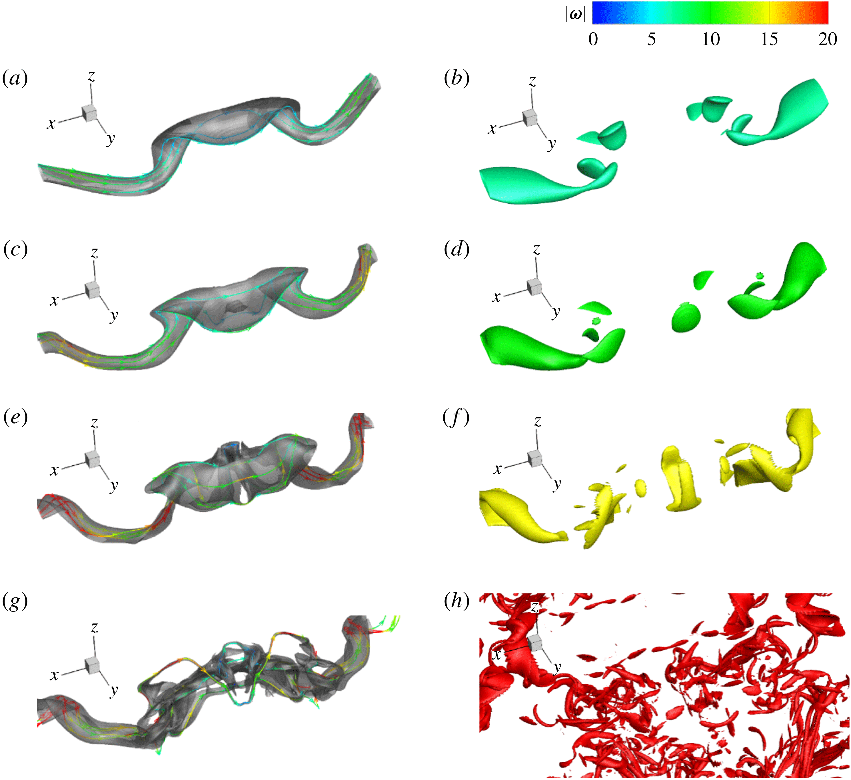
, the initially large-scale, blob-like vortex surfaces have evolved into tube-like structures in TG flows (see Yang & Pullin Reference Yang and Pullin2011). These vortex tubes are twisted and flattened either by self-induced dynamics or interactions with other tubes. Figure 7 shows the isosurfaces of
 $\hat{\unicode[STIX]{x1D719}}_{v}=0.5$
and varied
 $|\unicode[STIX]{x1D74E}|$
in a typical subdomain
 $[\unicode[STIX]{x03C0}/2,3\unicode[STIX]{x03C0}/2]\times [5\unicode[STIX]{x03C0}/8,\unicode[STIX]{x03C0}]\times [3\unicode[STIX]{x03C0}/2,7\unicode[STIX]{x03C0}/4]$
at
 $t=7.5$
in TG flows with four
 $Re$
from 400 to 3200. Here,
 $\hat{\unicode[STIX]{x1D719}}_{v}$
denotes the normalized VSF, which is implicitly determined by
 $\hat{M}(\hat{\unicode[STIX]{x1D719}}_{v}=\unicode[STIX]{x1D711},t)=\hat{M}(\unicode[STIX]{x1D719}_{v0}=\unicode[STIX]{x1D711},t=0)$
by searching the isocontour values
 $\hat{\unicode[STIX]{x1D719}}_{v}=\unicode[STIX]{x1D711}$
at a given time
 $t$
and
 $\unicode[STIX]{x1D719}_{v0}$
at
 $t=0$
which correspond to the same fluid mass
 $\hat{M}$
(see Peng & Yang Reference Peng and Yang2018).
With increasing
 $Re$
, the VSF isosurface becomes distorted and helical in figure 7, but it is still coherent. The curved and twisted vortex tubes are related to the intermittent statistics in turbulence (e.g. She et al.
Reference She, Jackson and Orszag1990). By contrast, the isosurface of
 $|\unicode[STIX]{x1D74E}|$
becomes broken and dispersed with increasing
 $Re$
. In particular, for the case of
 $Re=3200$
in which the energy spectrum is close to that of fully developed HIT in figure 2, the very scattered isosurfaces of
 $|\unicode[STIX]{x1D74E}|$
in figure 7(h) make it hard to identify coherent vortical structures.
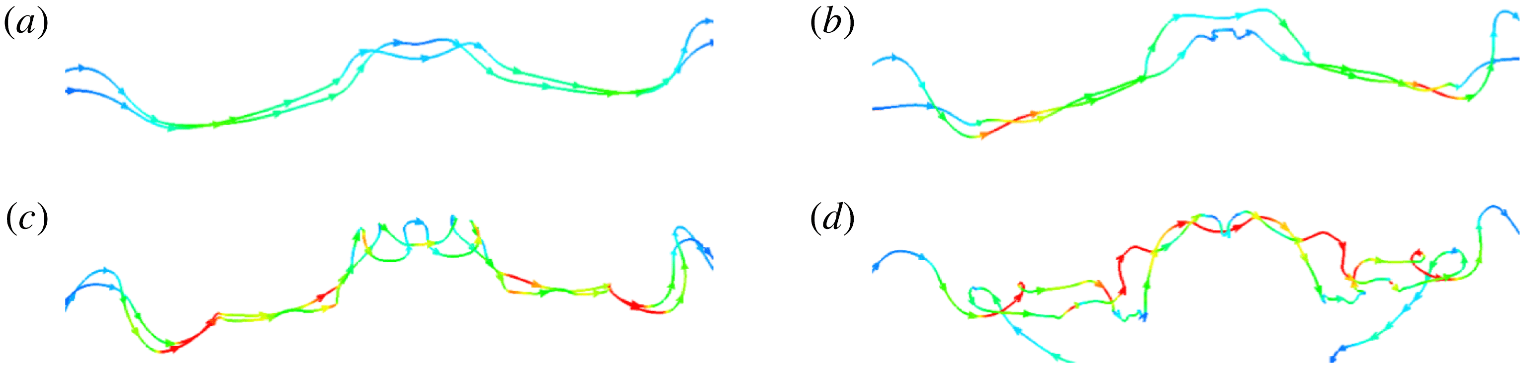
To further illustrate the visual differences between the isosurfaces of VSF and vorticity magnitude in figure 7, we extract two typical vortex lines in figure 8, which are integrated on the isosurfaces of
 $\hat{\unicode[STIX]{x1D719}}_{v}=0.5$
and colour coded by
 $|\unicode[STIX]{x1D74E}|$
. As
 $Re$
increases, the vortex lines become helical, consistent with the observation of VSF isosurfaces. The intermittent vorticity magnitude on the very distorted vortex lines at high
 $Re$
causes the broken isosurfaces of
 $|\unicode[STIX]{x1D74E}|$
in figure 7(h), which are sometimes referred to as ‘vortex worms’ in the literature. This visual breakdown of vortical structures, however, cannot characterize the geometry of highly twisted coherent vortex tubes, which may depend on the selection of the isocontour value of
 $|\unicode[STIX]{x1D74E}|$
.
Vortex lines in TG flows with different
 $Re$
at
 $t=7.5$
. These vortex lines are integrated on the isosurfaces of
 $\unicode[STIX]{x1D719}_{v}$
and colour coded by
 $|\unicode[STIX]{x1D74E}|$
with the same colour map as in figure 7. (a)
 $Re=400$
, (b)
 $Re=800$
, (c)
 $Re=1600$
, (d)
 $Re=3200$
.

5 Identification of vortex surfaces in decaying HIT
5.1 Isocontour values and VSF deviations
As demonstrated in §§ 3.3 and 4, we are able to construct relatively accurate and smooth VSFs in HIT by improving the VSF calculation with local optimization (3.5), and the VSF isosurface can effectively identify coherent and twisted vortex tubes. These indicate that the VSF is promising to identify the very convoluted vortex surfaces in fully developed HIT.
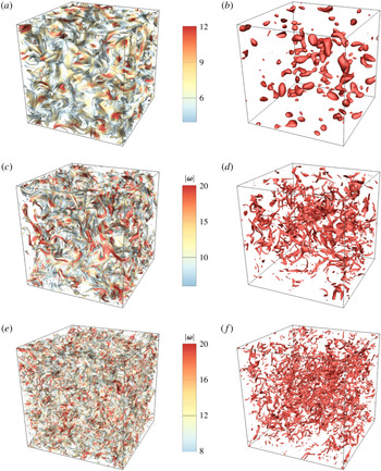
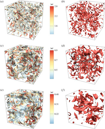
Isosurfaces of the VSF solution and vorticity magnitude in decaying HIT at six typical times listed in table 3 are shown in figures 9 and 10. The isosurfaces are colour coded by
 $|\unicode[STIX]{x1D74E}|$
, and the VSF isosurfaces with
 $|\unicode[STIX]{x1D74E}|<0.2|\unicode[STIX]{x1D74E}|_{max}$
are cut off for clarity, where
 $|\unicode[STIX]{x1D74E}|_{max}$
denotes the maximum vorticity magnitude in each instantaneous
 $|\unicode[STIX]{x1D74E}|$
.
Isosurfaces of
 $\unicode[STIX]{x1D719}_{v}$
and
 $|\unicode[STIX]{x1D74E}|$
in decaying HIT at
 $t=0$
, 1 and 2. The isocontour values and averaged VSF deviations of
 $\unicode[STIX]{x1D719}_{v}$
and
 $|\unicode[STIX]{x1D74E}|$
are listed in table 4. All the isosurfaces are colour coded by
 $|\unicode[STIX]{x1D74E}|$
, and the VSF isosurfaces with
 $|\unicode[STIX]{x1D74E}|<0.2|\unicode[STIX]{x1D74E}|_{max}$
are cut off for clarity. (a)
 $\unicode[STIX]{x1D719}_{v}$
and (b)
 $|\unicode[STIX]{x1D74E}|$
at
 $t=0$
; (c)
 $\unicode[STIX]{x1D719}_{v}$
and (d)
 $|\unicode[STIX]{x1D74E}|$
at
 $t=1$
; (e)
 $\unicode[STIX]{x1D719}_{v}$
and (f)
 $|\unicode[STIX]{x1D74E}|$
at
 $t=2$
.

Same as figure 9 except
 $t=10$
, 20 and 60. Some vortex lines are integrated on the isosurfaces at
 $t=20$
. (a)
 $\unicode[STIX]{x1D719}_{v}$
and (b)
 $|\unicode[STIX]{x1D74E}|$
at
 $t=10$
; (c)
 $\unicode[STIX]{x1D719}_{v}$
and (d)
 $|\unicode[STIX]{x1D74E}|$
at
 $t=20$
; and (e)
 $\unicode[STIX]{x1D719}_{v}$
and (f)
 $|\unicode[STIX]{x1D74E}|$
at
 $t=60$
.

The probability density function (p.d.f.) of the space-filling, normalized
 $\unicode[STIX]{x1D719}_{v}$
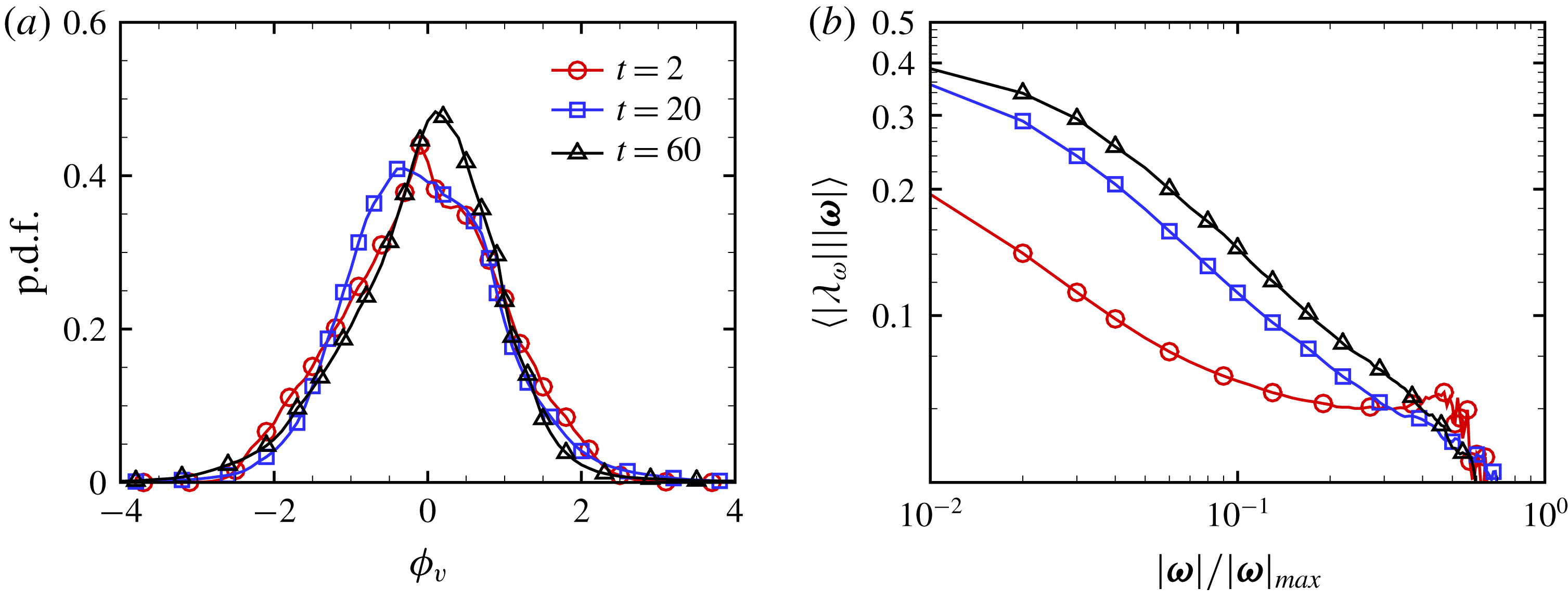
evolves from the initial double-delta distribution towards the standard Gaussian distribution in the pseudo-transport with numerical diffusion and local optimization, and it has a strong peak at zero with a slight skewness in figure 11(a). Thus we use the isocontour level
 $\unicode[STIX]{x1D719}_{v}=0$
to display the typical VSF isosurface which almost occupies the largest space of all the VSF isosurfaces. We remark that the subjective selection of isocontour levels is an important issue suffered by many vortex-identification methods. As listed in table 4, we fix the isocontour level
 $\unicode[STIX]{x1D719}_{v}=0$
in the visualization of VSFs, whereas we have to tune the threshold of normalized
 $|\unicode[STIX]{x1D74E}|$
to display the structures with similar characteristic sizes in figures 9 and 10.
Statistics of VSF solutions in decaying HIT at
 $t=2$
, 20 and 60. (a) Probability density function of
 $\unicode[STIX]{x1D719}_{v}$
; (b) volume average of
 $|\unicode[STIX]{x1D706}_{\unicode[STIX]{x1D714}}|$
conditioned on
 $|\unicode[STIX]{x1D74E}|$
.

Comparisons between the VSF and vorticity magnitude at the isocontour value selection and averaged VSF deviation in the vortex identifications in decaying HIT at six typical times.

On the faithful identification of vortex tubes and sheets, the VSF, due to its own definition, is superior to other vortex-identification methods. Table 4 compares the averaged VSF deviations between the VSF solution and vorticity magnitude in decaying HIT at six typical times, and
 $\langle |\unicode[STIX]{x1D706}_{\unicode[STIX]{x1D714}}|\rangle$
for
 $\unicode[STIX]{x1D719}_{v}$
is approximately five times less than that for
 $|\unicode[STIX]{x1D74E}|$
. As an example, some vortex lines are integrated on the isosurfaces at
 $t=20$
in figure 10(c,d). The large VSF deviation
 $\langle |\unicode[STIX]{x1D706}_{\unicode[STIX]{x1D714}}|\rangle \approx 30.8\,\%$
for the isosurface of
 $|\unicode[STIX]{x1D74E}|$
implies a significant misalignment between the isosurface and vortex lines in figure 10(d). The isosurface of
 $|\unicode[STIX]{x1D74E}|$
only displays strong vorticity regions, but loses directional information of vorticity, so it is hard to use in Lagrangian-like structure tracking based on the Helmholtz vorticity theorem owing to the large deviation from the vortex surfaces (see Yang & Pullin Reference Yang and Pullin2011). For comparison, the isosurface of
 $\unicode[STIX]{x1D719}_{v}$
displays the vortex tubes or sheets with a relatively small VSF deviation
 $\langle |\unicode[STIX]{x1D706}_{\unicode[STIX]{x1D714}}|\rangle \approx 5.5\,\%$
, so vortex lines are almost attached to the isosurface in figure 9(c), and the VSF isosurface colour coded by
 $|\unicode[STIX]{x1D74E}|$
captures both the magnitude and directional information of vorticity. Additionally, the geometry of the isosurfaces of other vortex-identification criteria based on the velocity gradient tensor is very similar to the isosurface of
 $|\unicode[STIX]{x1D74E}|$
.
The averaged VSF deviation conditioned on
 $|\unicode[STIX]{x1D74E}|$
in figure 11(b) implies that the construction of VSFs tends to be more accurate in the region with strong vorticity than in that with weak vorticity, because the visualization of vortex lines (She et al.
Reference She, Jackson and Orszag1990; Jimenez et al.
Reference Jimenez, Wray, Saffman and Rogallo1993) depicts that, in general, the vortex lines with large
 $|\unicode[STIX]{x1D74E}|$
are fairly straight while the vorticity vectors with small
 $|\unicode[STIX]{x1D74E}|$
have chaotic orientations.
5.2 Geometry of vortex surfaces in HIT
There is still considerable debate on the geometry of vortical structures in HIT (see Davidson Reference Davidson2004). Multi-scale diagnostic tools illustrate that structures of
 $|\unicode[STIX]{x1D74E}|$
evolve in a continuous distribution from blob-like and moderately stretched tube-like shapes at large scales, through a predominance of tube-like structures at intermediate scales, to highly stretched sheet-like structures at small scales (Ishihara et al.
Reference Ishihara, Kaneda, Yokokawa, Itakura and Uno2007; Bermejo-Moreno, Pullin & Horiuti Reference Bermejo-Moreno, Pullin and Horiuti2009; Leung, Swaminathan & Davidson Reference Leung, Swaminathan and Davidson2012).
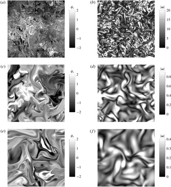
In figures 9 and 10, the VSF isosurfaces with strong and weak
 $|\unicode[STIX]{x1D74E}|$
, in general, tend to be tube-like and sheet-like, respectively. This observation is qualitatively consistent with that from isosurfaces of
 $|\unicode[STIX]{x1D74E}|$
. On the other hand, the VSF reveals more details of twisting and spirals of vortical structures than
 $|\unicode[STIX]{x1D74E}|$
. Plane cuts of the contour of
 $\unicode[STIX]{x1D719}_{v}$
in figure 12 depict the spiral structures in the contour of
 $\unicode[STIX]{x1D719}_{v}$
which are similar to passive scalars in HIT in Brethouwer, Hunt & Nieuwstadt (Reference Brethouwer, Hunt and Nieuwstadt2003) and Yang et al. (Reference Yang, Pullin and Bermejo-Moreno2010).
Plane cuts of VSF and vorticity magnitude contours in decaying HIT. (a)
 $\unicode[STIX]{x1D719}_{v}$
and (b)
 $|\unicode[STIX]{x1D74E}|$
at
 $t=2$
; (c)
 $\unicode[STIX]{x1D719}_{v}$
and (d)
 $|\unicode[STIX]{x1D74E}|$
at
 $t=20$
; (e)
 $\unicode[STIX]{x1D719}_{v}$
and (f)
 $|\unicode[STIX]{x1D74E}|$
at
 $t=60$
.

The theoretical analysis in Yang et al. (Reference Yang, Pullin and Bermejo-Moreno2010) suggests that a passive scalar field
 $\unicode[STIX]{x1D719}$
with vanishing diffusivity in stationary HIT tends to be attracted towards a VSF, but
 $\langle |\unicode[STIX]{x1D706}_{\unicode[STIX]{x1D714}}|\rangle$
is converged around 25 % owing to small but persistent viscous effects. The multi-scale geometric analysis of
 $\unicode[STIX]{x1D719}$
characterizes a geometrical progression from blobs through tubes to sheet-like structures with decreasing length scale in a space of reduced geometrical parameters. Compared with the statistical geometry of instantaneous
 $|\unicode[STIX]{x1D74E}|$
in HIT obtained by Bermejo-Moreno et al. (Reference Bermejo-Moreno, Pullin and Horiuti2009),
 $\unicode[STIX]{x1D719}$
tends to exhibit more prevalent sheet-like shapes at intermediate and small scales, which agrees with the visual difference between the VSF and
 $|\unicode[STIX]{x1D74E}|$
in figures 9, 10 and 12.
The generic spiral patterns of
 $\unicode[STIX]{x1D719}_{v}$
driven by frozen vorticity and the passive scalar driven by evolving velocity imply that the bundle of vortex lines can be highly twisted at large
 $Re_{\unicode[STIX]{x1D706}}$
, which is hypothesized as an elementary vortical structure in turbulence and is a key ingredient in the spiral vortex model for obtaining
 $E(k)\sim k^{-5/3}$
(see Lundgren Reference Lundgren1982; Pullin & Saffman Reference Pullin and Saffman1998). For comparison, the contours of large
 $|\unicode[STIX]{x1D74E}|$
in figure 12 are concentrated in blob-like regions, which correspond to the three-dimensional tube-like structures in figures 9 and 10 and appear not to illustrate the fine, internal structures in vortex tubes.
5.3 Implications of the morphology of vortex surfaces for energy cascade
The energy cascade is hypothesized to be related to the morphology of vortical structures at different scales. The isosurfaces of
 $\unicode[STIX]{x1D719}_{v}$
and
 $|\unicode[STIX]{x1D74E}|$
from
 $t=0$
to
 $2$
are shown in figure 9, when the flow evolves from a Gaussian random field into fully developed HIT. At
 $t=0$
, the isosurfaces of
 $\unicode[STIX]{x1D719}_{v}$
and
 $|\unicode[STIX]{x1D74E}|$
exhibit very different geometries, i.e. curved sheet-like structures and scattered blob-like structures in figures 9(a) and 9(b), respectively. The sheet-like vortex surfaces are rolled up into tube-like structures at
 $t=1$
, which is consistent with the observations of decaying HIT in Vincent & Meneguzzi (Reference Vincent and Meneguzzi1994) using vorticity vectors and with the transitional stage in TG flows in Yang & Pullin (Reference Yang and Pullin2011) using VSF.
The vortex tubes are then stretched and their characteristic scales decrease until the viscous effect becomes dominant to suppress the scale cascade. The smallest scale of vortex surfaces in figure 9 occurs around
 $t=2$
, which also corresponds to the time of the maximum dissipation rate in figure 1(b). The differences of the morphology of vortex surfaces from
 $t=0$
to
 $2$
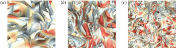
are also highlighted in the close-up views in figure 13. Instead of the isolated helical vortex tubes in TG flows in figure 7 and scattered short tubes of
 $|\unicode[STIX]{x1D74E}|$
in figure 9(f), the vortex tubes and sheets in HIT generally connect and tangle with neighbouring ones to constitute a complex network in figure 9(e). Subsequently, the scale of vortex surfaces begins to increase during the late evolution stage after
 $t=10$
in figure 10 owing to the viscous effect (see Hao et al.
Reference Hao, Xiong and Yang2019), when the turbulent kinetic energy has diminished below
 $1\,\%$
of the initial value. Moreover, appendix A explains that the statistical geometry of VSF isosurfaces is insensitive to the initial condition of (3.3), so the tangle of vortex tubes appears to be a global attractor in the chaotic vorticity system of fully developed HIT.
Close-up views of the VSF isosurfaces (from left to right:
 $t=0$
, 1 and 2) around the central region in figures 9(a), (c) and (e).

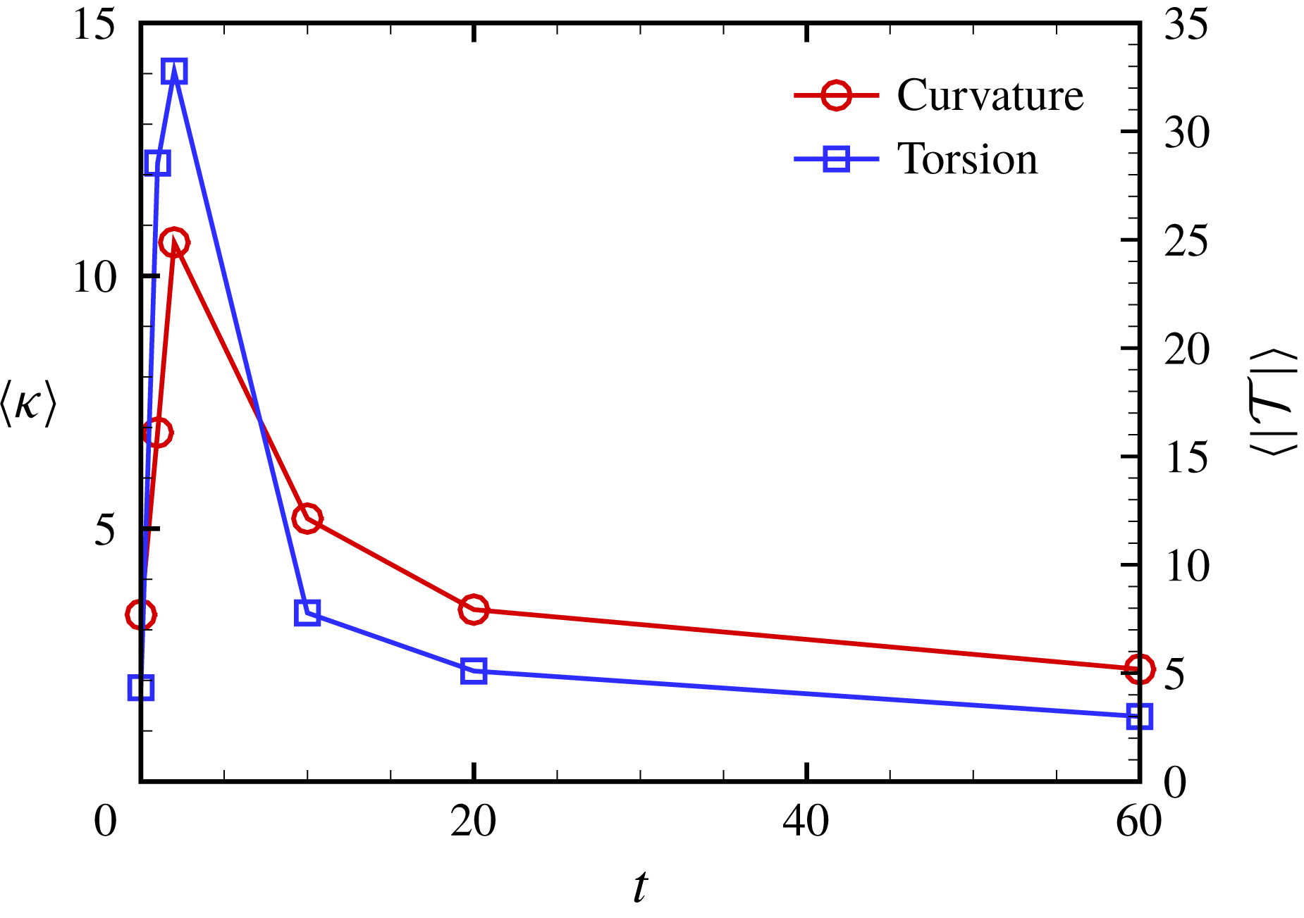
The deformation of VSF isosurfaces is accompanied by intensive stretching, folding and twisting of the attached vortex lines with increasing curvature and torsion. The local curvature and torsion of vortex lines are calculated from instantaneous
 $\unicode[STIX]{x1D74E}$
as
 $$\begin{eqnarray}\unicode[STIX]{x1D705}=\frac{|\unicode[STIX]{x1D74E}\times (\unicode[STIX]{x1D74E}\boldsymbol{\cdot }\unicode[STIX]{x1D735}\unicode[STIX]{x1D74E})|}{|\unicode[STIX]{x1D74E}|^{3}}\end{eqnarray}$$
and
 $$\begin{eqnarray}{\mathcal{T}}=\frac{\unicode[STIX]{x1D74E}\boldsymbol{\cdot }[\unicode[STIX]{x1D735}(\unicode[STIX]{x1D74E}\boldsymbol{\cdot }\unicode[STIX]{x1D735}\unicode[STIX]{x1D74E})]\boldsymbol{\cdot }[\unicode[STIX]{x1D74E}\times (\unicode[STIX]{x1D74E}\boldsymbol{\cdot }\unicode[STIX]{x1D735}\unicode[STIX]{x1D74E})]}{|\unicode[STIX]{x1D74E}\times (\unicode[STIX]{x1D74E}\boldsymbol{\cdot }\unicode[STIX]{x1D735}\unicode[STIX]{x1D74E})|^{2}},\end{eqnarray}$$
respectively. Figure 14 plots the temporal evolution of
 $\unicode[STIX]{x1D705}$
and
 $|{\mathcal{T}}|$
averaged over the isosurface of
 $\unicode[STIX]{x1D719}_{v}=0$
. The averaged curvature and torsion peak at
 $t\approx 2$
, which coincides with the occurrence of the maximum distortion of VSF isosurfaces in figures 9 and 10 and the maximum dissipation rate in figure 1(b). Hence, we speculate that the stretching and twisting of vortex surfaces/lines are correlated to the energy cascade in HIT, which is also supported by the VSF characterization of filtered HIT fields in appendix C.
Temporal evolution of the curvature and absolute value of torsion averaged over the VSF isosurface of
 $\unicode[STIX]{x1D719}_{v}=0$
.

Additionally, the understanding of vortex morphology depends on the structure-identification method. For example, in figure 10(a,b) at
 $t=10$
, the isosurface of
 $\unicode[STIX]{x1D719}_{v}$
displays a complex network of vortex surfaces as a tangle of long vortex tubes, whereas the isosurface of
 $|\unicode[STIX]{x1D74E}|$
displays clusters of short tube-like structures as ‘vortex worms’. Sometimes the energy cascade is characterized by the visual ‘breakdown’ of isosurfaces of
 $|\unicode[STIX]{x1D74E}|$
, as shown in the right columns of figures 9 and 10 and illustrated by blue patches in figure 15. However, this breakdown of isosurfaces of
 $|\unicode[STIX]{x1D74E}|$
is elusive in terms of vortex dynamics, because physically reasonable deformation of vortex lines and surfaces in energy cascade should be due to continuous processes such as stretching, twisting and reconnection, as illustrated by red patches in figure 15.
A schematic diagram of different views of the scale cascade of vortical structures in turbulence. Blue and red patches denote the isosurfaces of vorticity magnitude and VSF, respectively. Red lines with arrows denote vortex lines, dashed black lines with arrows denote the velocity induced by the vortex lines attached to vortex surfaces and grey arrows denote the background straining motion.

Therefore, as sketched in figure 15, the isosurface of
 $\unicode[STIX]{x1D719}_{v}$
appears to depict a more comprehensive picture than the isosurface of
 $|\unicode[STIX]{x1D74E}|$
of vortex dynamics in energy cascade, e.g. vortex twisting at small scales and rolling-up of vortex sheets. A similar visual difference between isosurfaces of
 $\unicode[STIX]{x1D719}_{v}$
and
 $|\unicode[STIX]{x1D74E}|$
is observed in TG flows in figure 7. For comparison, HIT has less isolated twisted vortex tubes in figures 9 and 10, because vortex surfaces in HIT are superposed and tangled together with strong interactions.
6 Conclusions
We extend the VSF to fully developed turbulence to identify vortex tubes and sheets. These elementary vortical structures consisting of vortex lines are hypothesized to be important in turbulence dynamics, but they cannot be accurately identified using most of the existing structure-identification methods.
The VSF at an instant is constructed by solving a pseudo-transport equation convected by a given instantaneous vorticity obtained from DNS. Since the VSF solution tends to be non-smooth in the pseudo-transport owing to the persistent straining of scalar structures driven by the frozen vorticity in turbulence, we develop a local optimization algorithm to minimize the hybrid constraint for achieving both satisfactory VSF deviation and smoothness of VSF solutions.
In the numerical construction of VSFs in decaying HIT with moderate numbers of VSF grid points, the volume-averaged VSF deviation can be controlled to a level as small as
 $\langle |\unicode[STIX]{x1D706}_{\unicode[STIX]{x1D714}}|\rangle \leqslant 8.0\,\%$
, and this deviation can be further reduced by increasing the grid resolution for VSFs. We choose the isosurface of fixed
 $\unicode[STIX]{x1D719}_{v}=0$
to identify typical vortex surfaces and use the spatial delta-correlated scalar field as the initial condition in the pseudo-evolution. These choices are adopted in all the VSF constructions in HIT to avoid the subjectivity in structure identification.
In the visualization of VSF isosurfaces in decaying HIT, the initial curved vortex sheets first evolve into vortex tubes, and then the tubes are stretched with decreasing length scale. At the fully developed turbulent stage, in general, the VSF isosurfaces tend to form tube-like structures with a large vorticity magnitude and small VSF deviation, and the tangled vortex tubes constitute a complex network. Some vortex tubes exhibit helical geometry, which reveals the important role of vortex twisting in the generation of small-scale structures in energy cascade and supports Lundgren’s spiral vortex model. The occurrence of maximum curvature and torsion of vortex lines attached to the VSF isosurfaces coincides with that of the maximum dissipation rate in HIT, so the stretching and twisting of vortex surfaces/lines are correlated to the energy cascade. At the later decaying stage, the size of the vortex tubes is increased due to the dominate viscous effect.
By contrast, the VSF deviation for the isosurface of vorticity magnitude can be as large as
 $\langle |\unicode[STIX]{x1D706}_{\unicode[STIX]{x1D714}}|\rangle \approx 30\,\%$
, which is manifested as the significant misalignment between the isosurface of
 $|\unicode[STIX]{x1D74E}|$
and vortex lines. We demonstrate that the large variation of
 $|\unicode[STIX]{x1D74E}|$
on the same vortex surface causes the visual ‘breakdown’ of the isosurface of
 $|\unicode[STIX]{x1D74E}|$
as ‘vortex worms’ in HIT and TG flows, so the isosurface of
 $|\unicode[STIX]{x1D74E}|$
cannot accurately identify complete and coherent vortex surfaces in turbulence.
The pseudo-transport with the local optimization developed in the present study can be applied to construct VSFs in arbitrary three-dimensional velocity fields as a general structure-identification method. We remark that the VSF constructions at a series of successive time instants are not ensured to display a Lagrangian-like evolution of the vortex surface owing to the non-uniqueness of VSF solutions (Xiong & Yang Reference Xiong and Yang2017), but the constructed VSF at a time instant can be used as an initial condition in the evolution of VSFs using the two-time method (Yang & Pullin Reference Yang and Pullin2011). In future work, the combination of the present VSF construction and the further improvement of the computational efficiency of the VSF evolution algorithm and the numerical regularization near vorticity nulls (Hao et al. Reference Hao, Xiong and Yang2019) is expected to be applied to compute the evolution of VSFs in fully developed turbulence for elucidating the energy cascade from a Lagrangian view.
Acknowledgements
Y.Y. thanks Y. Zhao and W. Tong for their comments. Numerical simulations were carried out on the TH-2A supercomputer in Guangzhou, China. This work has been supported in part by the National Natural Science Foundation of China (grant nos 11522215, 91541204 and 91841302).
Appendix A. Uniqueness of the VSF solution in HIT
In principle, the VSF solution for an instantaneous velocity–vorticity field is not unique, because the first-order linear homogeneous partial differential equation (3.1) may have multiple independent solutions (see Evans Reference Evans2010). It is possible to add additional constraints to make the solution of (3.1) unique, as discussed for simple shear flows and transitional channel flows in Xiong & Yang (Reference Xiong and Yang2017). For more general flows, if the flow field is chaotic, different VSF-construction methods identify similar structures. For example, for the TG flow at
 $t=7.5$
, both the two-time method and the boundary-constraint method construct nearly identical vortex tubes (see Xiong & Yang Reference Xiong and Yang2017). Therefore, the coherent vortex tubes appear to be a global attractor in the set of nonlinear characteristic equations of (3.3) with chaotic vorticity. This global attractor is a bounded set of numerical values towards which a system tends to evolve, for a wide variety of initial conditions of the system.
Since the vortex lines in a turbulent flow are highly chaotic, the VSFs constructed by different methods and initial conditions should have structural similarity. Thus although the initial field
 $\unicode[STIX]{x1D719}_{v0}$
of (3.3) is arbitrary, the statistical geometry of converged VSF solutions is insensitive to the choice of
 $\unicode[STIX]{x1D719}_{v0}$
. In the decaying HIT at
 $t=20$
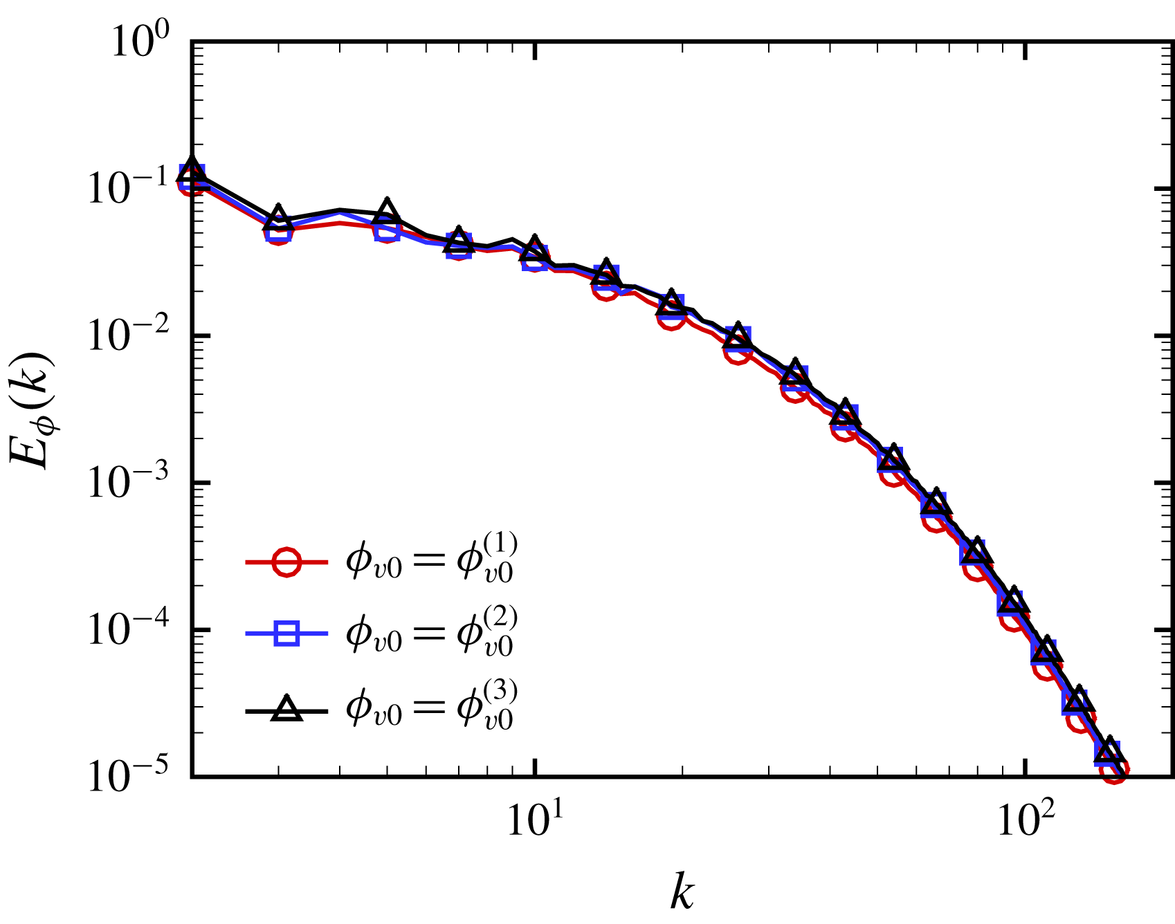
, figure 16 shows nearly identical scalar spectra of the VSF solutions calculated from three independent initial conditions, the spatial delta-correlated field
 $\unicode[STIX]{x1D719}_{v0}^{(1)}$
,
 $\unicode[STIX]{x1D719}_{v0}^{(2)}=\cos x\cos y\cos z$
and
 $\unicode[STIX]{x1D719}_{v0}^{(3)}=\sin x\sin y\sin z$
. This indicates that the pseudo-transport with local optimization restores uniqueness of the VSF solution, so the tangle of vortex tubes appears to be the robust geometry of vortex surfaces or a global attractor of chaotic vortex lines in HIT.
Scalar spectra of the VSF solutions calculated from three independent initial conditions, the spatial delta-correlated field
 $\unicode[STIX]{x1D719}_{v0}^{(1)}$
,
 $\unicode[STIX]{x1D719}_{v0}^{(2)}=\cos x\cos y\cos z$
and
 $\unicode[STIX]{x1D719}_{v0}^{(3)}=\sin x\sin y\sin z$
, in decaying HIT at
 $t=20$
.

Appendix B. Effects of local optimization on VSF construction
We provide a two-dimensional example to illustrate the effects of the local optimization, described in § 3.2, on the smoothness of VSF solutions in VSF construction. We construct a ‘VSF’ or a first integral (see He & Yang Reference He and Yang2016) for a given two-dimensional divergence-free vector field
 $$\begin{eqnarray}\unicode[STIX]{x1D74E}=(\unicode[STIX]{x1D714}_{x},\unicode[STIX]{x1D714}_{y})=(\sin x\cos y,-\cos x\sin y).\end{eqnarray}$$
The pseudo-transport equation (3.3) is solved on uniform grid points
 $N_{\unicode[STIX]{x1D719}}^{2}=128^{2}$
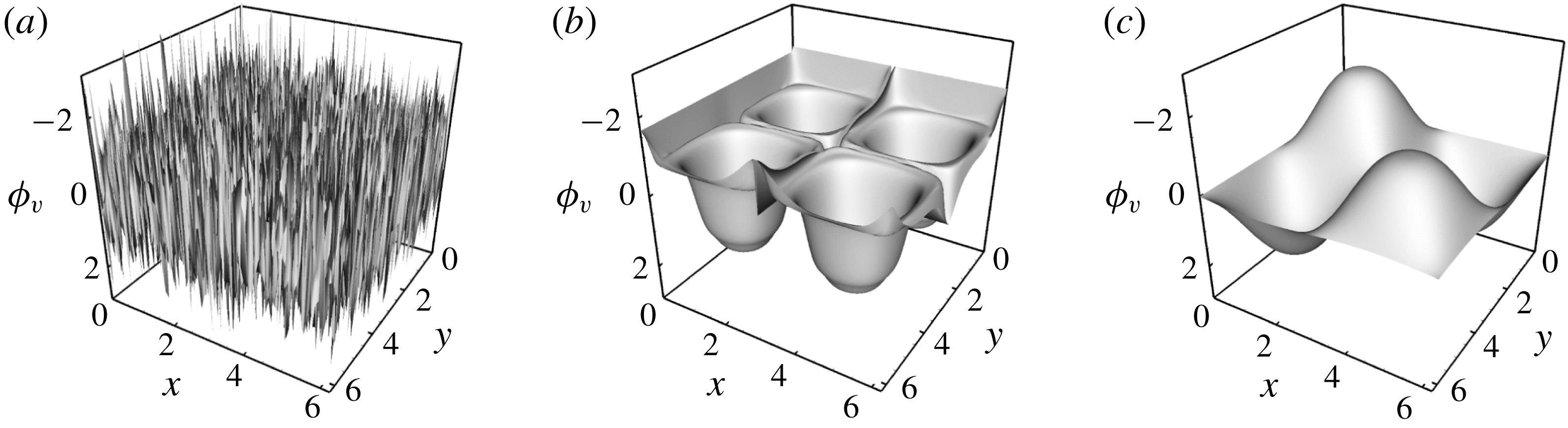
. The initial condition is a delta-correlated random field shown in figure 17(a).
Contours of
 $\unicode[STIX]{x1D719}_{v}$
in the two-dimensional pseudo-evolution. (a)
 $\unicode[STIX]{x1D70F}/T_{v}=0$
; (b)
 $\unicode[STIX]{x1D70F}/T_{v}=10$
, without local optimization; (c)
 $\unicode[STIX]{x1D70F}/T_{v}=10$
, with local optimization.

We apply three strategies to study the influence of the local optimization (3.5) and the weighting factor
 $\unicode[STIX]{x1D701}$
in (3.4) on the quality of VSF solutions: (i) hybrid optimization: local optimization with adaptive
 $\unicode[STIX]{x1D701}$
determined by (3.6); (ii) gradient optimization: local optimization with fixed
 $\unicode[STIX]{x1D701}=1$
; (iii) without local optimization.
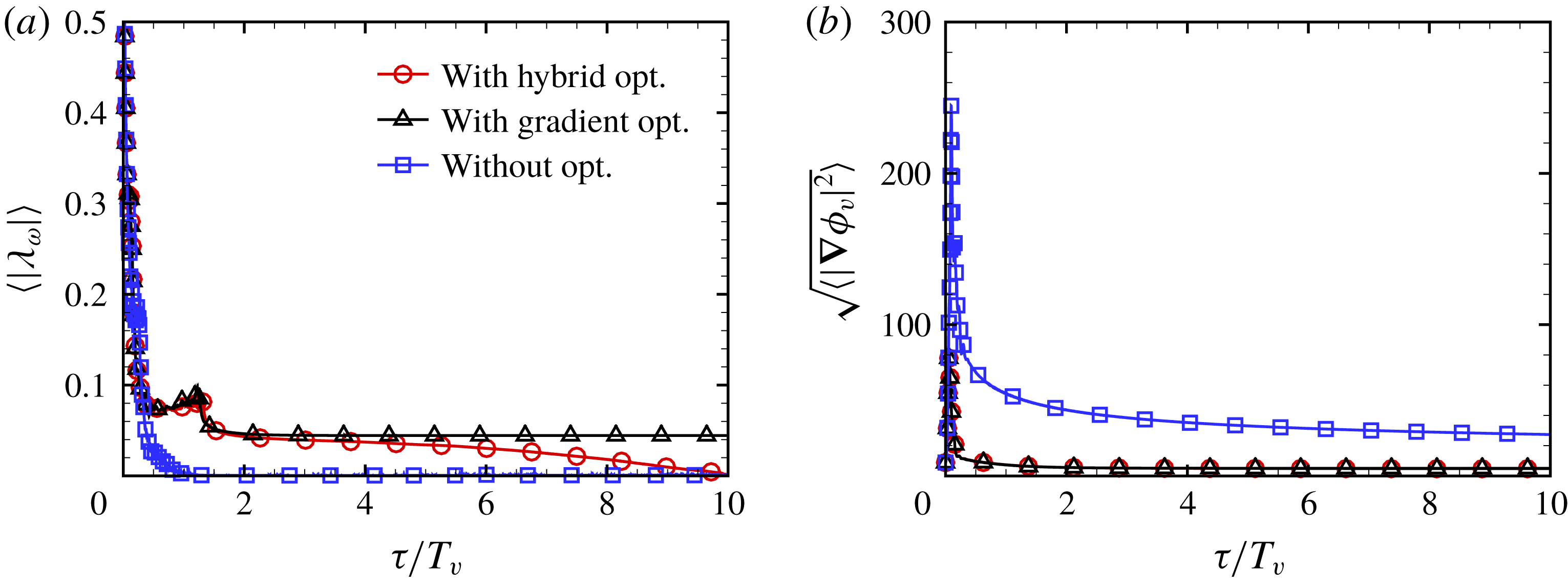
The pseudo-evolutions of the averaged VSF deviation and gradient magnitude in the VSF construction with different optimization strategies are shown in figure 18. If the VSF is calculated without local optimization, the VSF gradient magnitude can be large, although the VSF deviation is small. This results in the non-smooth VSF solution, shown as the spiky structures in the solution contour in figure 17(b). On the other hand, if the VSF is calculated with the gradient optimization, although the smoothness of the VSF solution is significantly improved, the VSF deviation is relatively large. Finally, we find that the hybrid optimization can balance the accuracy and smoothness of the VSF solution to obtain the converged solution with both small
 $\langle |\unicode[STIX]{x1D706}_{\unicode[STIX]{x1D714}}|\rangle$
and
 $\sqrt{\langle |\unicode[STIX]{x1D735}\unicode[STIX]{x1D719}_{v}|^{2}\rangle }$
, shown as the smooth solution contour in figure 17(c).
The pseudo-evolution of the averaged VSF deviation and gradient magnitude in the two-dimensional example. (a)
 $\langle |\unicode[STIX]{x1D706}_{\unicode[STIX]{x1D714}}|\rangle$
; (b)
 $\sqrt{\langle |\unicode[STIX]{x1D735}\unicode[STIX]{x1D719}_{v}|^{2}\rangle }$
.

Appendix C. VSFs of filtered HIT fields
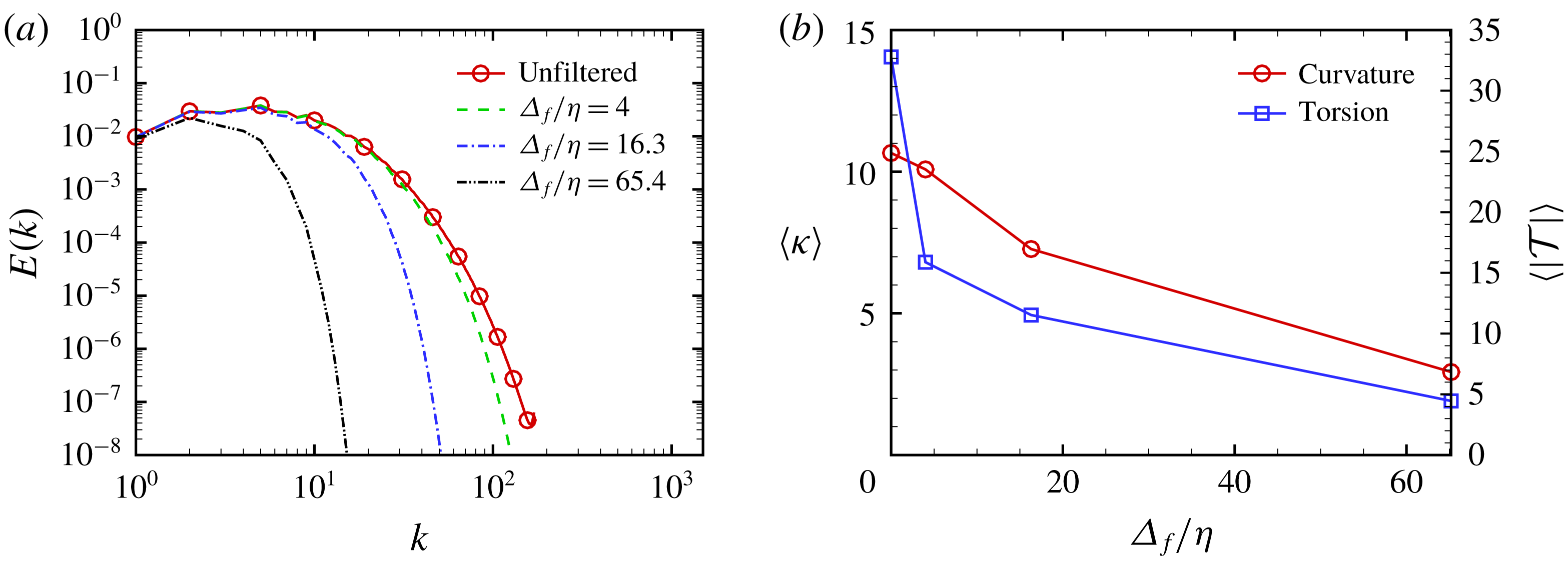
In order to distinguish how the different scales are represented by VSF structures, we filter the HIT filed at
 $t=2$
, which corresponds to the maximum dissipation rate, using a low-pass Gaussian filter. The filtered velocity is obtained as
 $$\begin{eqnarray}\widetilde{\boldsymbol{u}}(\boldsymbol{x};\unicode[STIX]{x1D6E5}_{f})={\mathcal{F}}^{-1}\{{\mathcal{F}}\{\boldsymbol{u}\}\widehat{G}(k;\unicode[STIX]{x1D6E5}_{f})\},\end{eqnarray}$$
where
 ${\mathcal{F}}$
and
 ${\mathcal{F}}^{-1}$
respectively denote Fourier and inverse Fourier transforms, the Gaussian kernel function (Pope Reference Pope2000) is defined by
 $\widehat{G}(k;\unicode[STIX]{x1D6E5}_{f})=\exp (-k^{2}\unicode[STIX]{x1D6E5}_{f}^{2}/24)$
and the filter widths are selected as
 $\unicode[STIX]{x1D6E5}_{f}=4\unicode[STIX]{x1D702}$
,
 $\unicode[STIX]{x1D6E5}_{f}=L_{e}/2\approx 16.3\unicode[STIX]{x1D702}$
and
 $\unicode[STIX]{x1D6E5}_{f}=2L_{e}\approx 65.4\unicode[STIX]{x1D702}$
. The spectra of the filtered velocity fields are shown in figure 19(a), and ratios of the filtered total kinetic energy to the unfiltered
 $E_{tot}$
are
 $96.2\,\%$
,
 $67.9\,\%$
and
 $17.4\,\%$
.
(a) Energy spectra and (b) the curvature and absolute value of torsion averaged over the VSF isosurface of
 $\widetilde{\unicode[STIX]{x1D719}}_{v}=0$
in filtered HIT fields with various filter widths at
 $t=2$
.

We calculate filtered VSFs
 $\widetilde{\unicode[STIX]{x1D719}}_{v}(\unicode[STIX]{x1D6E5}_{f})$
based on the filtered vorticity field
 $\widetilde{\unicode[STIX]{x1D74E}}(\unicode[STIX]{x1D6E5}_{f})=\unicode[STIX]{x1D735}\times \widetilde{\boldsymbol{u}}(\unicode[STIX]{x1D6E5}_{f})$
using the method described in § 3.2, and the averaged VSF deviations for all the filtered VSFs are less than
 $10\,\%$
. In figure 20, with increasing
 $\unicode[STIX]{x1D6E5}_{f}$
, we observe that the characteristic length scales of
 $\widetilde{\unicode[STIX]{x1D719}}_{v}(\unicode[STIX]{x1D6E5}_{f}=4\unicode[STIX]{x1D702})$
,
 $\widetilde{\unicode[STIX]{x1D719}}_{v}(\unicode[STIX]{x1D6E5}_{f}=L_{e}/2)$
and
 $\widetilde{\unicode[STIX]{x1D719}}_{v}(\unicode[STIX]{x1D6E5}_{f}=2L_{e})$
increase and the structures become less distorted. Comparing this trend with the VSF isosurfaces in figures 9 and 10, the structural evolution of VSFs with time in decaying HIT is similar to filtering a HIT with increasing
 $\unicode[STIX]{x1D6E5}_{f}$
.
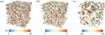
Isosurfaces of
 $\widetilde{\unicode[STIX]{x1D719}}_{v}=0$
in filtered HIT at
 $t=2$
with filter widths (a)
 $\unicode[STIX]{x1D6E5}_{f}/\unicode[STIX]{x1D702}=4$
, (b)
 $\unicode[STIX]{x1D6E5}_{f}/\unicode[STIX]{x1D702}=16.3$
and (c)
 $\unicode[STIX]{x1D6E5}_{f}/\unicode[STIX]{x1D702}=65.4$
. All the isosurfaces are colour coded by
 $|\widetilde{\unicode[STIX]{x1D74E}}|$
, and the VSF isosurfaces with
 $|\widetilde{\unicode[STIX]{x1D74E}}|<0.2|\widetilde{\unicode[STIX]{x1D74E}}|_{max}$
are cut off for clarity.

Figure 19(b) plots the variation of the curvature and absolute value of torsion of vortex lines averaged over the isosurface of
 $\widetilde{\unicode[STIX]{x1D719}}_{v}=0$
in filtered HIT fields at
 $t=2$
, and both decrease with
 $\unicode[STIX]{x1D6E5}_{f}$
. This implies that the vortex stretching and twisting contribute to the small-scale fluctuations in HIT. In particular, filtered HIT with
 $\unicode[STIX]{x1D6E5}_{f}=4\unicode[STIX]{x1D702}$
only loses 3.8 % of
 $E_{tot}$
, but the surface-averaged
 $|{\mathcal{T}}|$
drops from 14 to 6.8, which highlights the contribution of twisting of vortex lines to the turbulent fluctuations around the Kolmogorov scale.