I. INTRODUCTION
The burning of fossil fuels contributes to the pollution of the environment and to the global warming. Besides, petrol will be exhausted in a few decades. Many efforts are now dedicated to find clean fuels that could replace gasoline in transportation vehicles, and hydrogen is considered as a firm candidate.Reference Ogden1 Those cars will use an electric motor based on a hydrogen fuel cell.2 The hydrogen gas coming from the storage tank reacts in the cell with atmospheric oxygen producing an electric current, and the only emission from the reaction is pure water. The hydrogen cars will have some advantages with respect to gasoline cars and cars moved by electric batteries. Hydrogen is very abundant and can be produced from water by electrolysis. The recharge times will be substantially smaller than the recharge times for electric battery cars. In addition, the technology of hydrogen fuel cells is well developed.2 The energy content per mass of hydrogen, 120 MJ/kg, is higher than that of gasoline, 44 MJ/kg. However, hydrogen is a gas, and its energy content per volume at room conditions, 0.01 MJ/L, is much smaller than that of gasoline, 35 MJ/L. In gaseous hydrogen, at normal conditions of pressure and temperature, the average distance between molecules is about 3.3 nm, and 1 kg of hydrogen occupies the volume of a soccer goal. Therefore, the bottleneck of the hydrogen car technology is to find an efficient way to store hydrogen. In other words, the problem is how to store in a small tank 5 kg of hydrogen to run the car for about 600 km.
The short-term targets proposed by the U.S. Department of Energy (DOE) in September 2009, which would permit using hydrogen as a fuel in onboard applications, are: a gravimetric storage capacity of at least 5.5% of hydrogen in weight and a volumetric capacity of more than 0.040 kg of hydrogen per liter at room temperature and moderate pressures.3 The gravimetric capacity of the supporting or adsorbent material, or weight percent (wt%) of stored hydrogen, is:
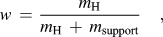 $$w\, = \,{{m_{\rm{H}} } \over {m_{\rm{H}} \, + \,m_{{\rm{support}}} }}\quad,$$
where m H is the mass of stored hydrogen and m support is the mass of the supporting material. The volumetric capacity V c equals to m H divided by the volume of the supporting material, V support:
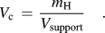 $$V_{\rm{c}} \, = \,{{m_{\rm{H}} } \over {V_{{\rm{support}}} }}\quad.$$
In addition, the storage should be reversible at room conditions. With these targets fulfilled, the hydrogen cars would have a similar autonomy range as the present gasoline cars.
Hydrogen can be stored in different ways.Reference Cabria, López, Alonso and Sattler4 Gaseous hydrogen can be stored in steel tanks at high pressures of 350–700 bar, and this is the storage technology used in the present hydrogen car prototypes. The main problems are the large weight and volume of the tanks and the energy required to compress the hydrogen gas. Liquid hydrogen is usually stored in cryogenic tanks at temperatures around 20 K. The energy content of liquid hydrogen is high, 8.4 MJ/L. This method reaches hydrogen storage capacities of 20 wt% and 0.030 kg/L, but the disadvantages are the boil-off losses and the need of strict insulation of the cryogenic tanks. In addition, a substantial amount of energy is used in the liquefaction of hydrogen. Other possibility is to store hydrogen as part of other liquids, such as NaBH4solutions, organic liquids, and ammonia. The usable hydrogen is produced by a chemical reaction, but the problem is that the other reaction products should be removed and recycled off-board. Hydrogen storage in solid materials is a safer method than gas and liquid storage. Two types of promising solid materials are metal hydrides and porous materials. Metal hydrides store atomic hydrogen dissolved in the crystal lattice of the metal. However, the storage process is not easily reversible because hydrogen is strongly bound in the hydride, and a large amount of energy is required to release the hydrogen.
There are several types of porous materials that have been studied for storing hydrogen and other gases: porous carbons,Reference Cabria, López, Alonso and Sattler4 metal organic frameworks,Reference Wong-Foy, Matzger and Yaghi5 zeolites,Reference Langmi, Walton, Al-Mamouri, Johnson, Book, Speight, Edwards, Gameson, Anderson and Harris6 clathrate hydrates,Reference Mao, Mao, Goncharov, Struzhkin, Guo, Hu, Shu, Hemley, Somayazulu and Zhao7 and microporous organic polymers.Reference McKeown, Budd and Book8 The storage mechanism in these materials is the molecular adsorption of H2 on the pore walls. Two quantities are then important to determine the storage capacity: the specific surface area (SSA) of the porous material, i.e., the surface area of the pore walls per gram of material, and the adsorption energy of H2. Porous materials show large SSAs of several thousand m2/g. With respect to adsorption energies on the pore surfaces, E ad, thermodynamic estimations by Li et al.Reference Li, Furuta, Goto, Ohashi, Fujiwara and Yip9 indicate that the values of E ad that would led to an efficient adsorption–desorption cyclic process at moderate pressures and 300 K are in the range 0.3–0.4 eV/molecule. A different estimation by Bhatia and MyersReference Bhatia and Myers10 gives a value of 0.16 eV/molecule at moderate pressures and 298 K. This is a narrow window intermediate between typical physisorption and chemisorption energies. None of the current hydrogen storage methods and none of the known solid materials meet the DOE targets.
In this article, we review recent work on the storage of hydrogen on nanoporous carbons. The structure of these materials is considered in Sec. II. Section III presents a theoretical discussion of the interaction of molecular hydrogen with graphitic surfaces, representative of the surface of the carbon pores. Section IV introduces a thermodynamic model to calculate the amount of hydrogen stored in porous carbons as a function of temperature and pressure. Section V investigates the effect of doping the material with metallic atoms and nanoparticles. Finally, Sec. VI presents the conclusions.
II. ATOMIC STRUCTURE OF NANOPOROUS CARBONS
The term nanoporous carbons embraces a broad class of carbon materials, including activated carbons (ACs),Reference Linares-Solano, Jordá-Beneyto, Kunowsky, Suárez-García, Cazorla-Amorós, Terzyk, Gauden and Kowalczyk11 carbide-derived carbons (CDCs),Reference Dash, Yushin and Gogotsi12 schwarzites,Reference Lenosky, Gonze, Teter and Elser13 carbon nanofoams,Reference Barborini, Piseri, Milani, Benedek, Ducati and Robertson14, Reference Benedek, Vahedi-Tafreshi, Baroni, Piseri, Milani, Ducati and Robertson15 carbon nanotubes,Reference Dresselhaus, Dresselhaus and Avouris16 carbon nanohorns,Reference Iijima, Yudasaka, Yamada, Bandow, Suenaga, Kokai and Takahashi17 etc., which present a highly porous structure with pores of nanometric sizes. These materials exhibit low densities, high SSAs, and high porosities. These properties make them attractive for many applications, like filtering membranes, coatings, catalysis, supercapacitors, and the storage of gases. Nanoporous carbons can be synthesized from precursor materials following different treatments: chemical vapor deposition, pyrolysis, chemical attack, activation, etc. Spongy carbon has been produced by cluster beam deposition.Reference Barborini, Piseri, Milani, Benedek, Ducati and Robertson14, Reference Benedek, Vahedi-Tafreshi, Baroni, Piseri, Milani, Ducati and Robertson15 ACs are produced from organic precursors (wood, coals, organic polymers, etc.), which are activated by physical or chemical procedures.Reference Linares-Solano, Jordá-Beneyto, Kunowsky, Suárez-García, Cazorla-Amorós, Terzyk, Gauden and Kowalczyk11 CDCs are produced from metallic carbides,Reference Dash, Yushin and Gogotsi12 extracting the metal atoms by a chemical process of chlorination:
 $${\rm{MC}}\, + \,{x \over 2}{\rm{Cl}}_{\rm{2}} \to {\rm{MCl}}_x \, + \,{\rm{C\quad,}}$$
at temperatures between 873 and 1473 K. Here, MC represents a metal carbide (TiC, ZrC, etc.). Upon removal of the metal atoms from the carbide, the sublattice of carbon atoms collapses into a completely different structure, but the material formed keeps the same macroscopic volume of the starting carbide.Reference Gogotsi, Nikitin, Ye, Zhou, Fischer, Yi, Foley and Barsoum18 Boron and silicon carbides can also be used as precursors. The properties of these materials can be tuned by careful selection of the production conditions and posttreatment of the samples. The size of the pores depends (i) on the precursor carbide, which determines the distribution of carbon atoms in the carbide, (ii) the synthesis temperature, and (iii) the presence of catalytic particles. A low chlorination temperature (<873 K) leads to CDCs with nanopores of near uniform size. Raising the synthesis temperature results in an increase of the average pore size and a broadening of the pore size distribution. CDCs have been synthesized with SSAs up to 2300 m2/g and pore volume fractions up to 84% of the volume of the material. The microstructure of the CDCs has been investigated using Raman spectroscopy and high-resolution transmission electron microscopy (TEM).Reference Yushin, Dash, Jagiello and Gogotsi19 At low production temperatures, about 673 K, the CDCs look completely amorphous, and graphite fringes are not distinguishable in the TEM images. At 1073 K, the carbon atoms reorganize to form curved graphene-like sheets, and at higher production temperatures, about 1473 K, small ribbons of graphite, a few layers thick, develop.
Computational studies of the structure of ACs and CDCs have been published recently.Reference Peng and Morris20, Reference López, Cabria and Alonso21 To simulate disordered porous carbons, Peng and MorrisReference Peng and Morris20 modeled the interaction between the carbon atoms with the empirical potential developed by Tersoff.Reference Tersoff22 This potential has a many-body character and represents well the covalent bonding between carbon atoms in diamond and graphite. Peng and Morris first equilibrated liquid carbon at 6000 K for 175 ps and then slowly quenched the structures to 300 K while keeping the carbon density constant. Cells containing 4000 carbon atoms and periodic boundary conditions were utilized in the simulations. The average densities of the simulated materials varied between 1.25 and 1.80 g/cm3. The computer simulations indicate the formation of graphitic segments, in agreement with the diffraction experiments from ACs.Reference Konnert and Dantonio23, Reference Kaneko, Ishii, Ruike and Kuwabara24 Those carbon densities are smaller than the densities of typical graphites (2.09–2.23 g/cm3), although larger than the densities of CDCs.
We have also used the Tersoff potential to simulate the structure of a nanoporous CDC obtained from ZrC precursor.Reference López, Cabria and Alonso21 This potential was combined with a long-range many-body potential due to Nordlund et al.Reference Nordlund, Keinonen and Mattila25 accounting for the weak interaction between adjacent layers in graphite. We call this the Tersoff–Nordlund potential for further reference. Then, molecular dynamics (MD) simulations of the collapse of the carbon structure giving rise to the porous structure of the CDCs were performed. The simulation cells are large, containing more than 60,000 carbon atoms, and the simulation times run up to 2500 ps. These conditions are required for a sensible comparison with the experimental results. The simulations have been performed at constant temperature, T, constant number of particles, N, and constant volume V. Therefore, the macroscopic carbon density, fixed equal to the experimental value for the carbon density skeleton in zirconium carbide, 0.77 g/cm3, remains constant along the simulation.
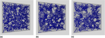
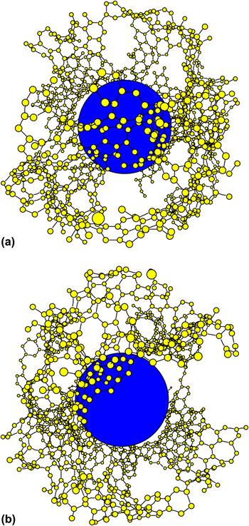
The MD simulations begin just after the extraction of the metal atoms from the carbide. We assume that the initial structure of the system of carbon atoms is close to that of the carbon face-centered-cubic sublattice in the precursor Zr carbide. In practice, we generate the initial configuration by slightly displacing atoms from their fcc positions and giving the atoms velocities a Maxwellian distribution corresponding to the selected temperature. This temperature is the parameter that controls the extent and speed of the structural transformations experienced by the carbon system and should not be identified with the chlorination temperature in the experiments, which controls the extraction of the metal from the carbide. The initial configuration is unstable and the carbon structure immediately collapses. After about 5 ps, small interconnected nanographene layers begin to grow, and after 20 ps, the main characteristics of the CDC structure are already apparent: a porous structure formed by interconnected nanopores of irregular shape and nonuniform size. The walls of the pores are graphite-like networks of carbon atoms, and the thickness of each of those walls is just one atomic layer. However, the honeycomb network of the walls contains many defects. As the simulation progresses, many defects are annealed out and the nanographene layers forming the pore walls grow larger. The structure obtained at a simulation temperature of 3010 K is shown in Fig. 1. The three panels correspond to three snapshots taken at times t = 5 ps, t = 20 ps, and t = 200 ps. In that simulation, the cell has the form of a cube with side length equal to 117.45 Å and contains 62,500 carbon atoms. However, to improve the visualization of the structure of the CDC, Fig. 1 shows a depth of 25 Å only. Nanographene layers begin to grow after 5 ps, the main features of the porous structure can already be seen after 20 ps, and at 200 ps, many defects in the graphene walls of the pores have annealed out, although a substantial number of defects are still present. The porous structure and the graphitic-like network forming the pore walls are clearly seen. A detail of a typical pore is shown in Fig. 2. In this case, the simulation was run at 2010 K, and many defects can be seen in the pore walls.
Structure of a CDC, obtained in a MD simulation run for 200 ps at a temperature of 3010 K. The precursor is ZrC. The periodic simulation cell contains 62,500 atoms. The cell has a length of 117.45 Å in each direction, but a depth of only 25 Å is shown for clarity. The three panels represent snapshots of the structure, taken at times t = 5 ps (a), t = 20 ps (b), and t = 200 ps (c), during the simulation.

Panels (a) and (b) show two views of a pore in a CDC, obtained in a MD simulation run for a time of 200 ps at a temperature of 2100 K. The periodic simulation cell contains 62,500 atoms. The central sphere helps to visualize the empty volume of the pore.

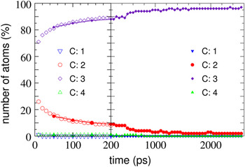
In a graphene layer, the carbon atoms are arranged in a hexagonal honeycomb ring pattern, in which the atoms are 3-fold coordinated. This structure arises from the sp 2 hybridization of the electronic orbitals of the carbon atoms. On the other hand, 2-fold coordination occurs at the edges of graphene ribbons. Figure 3 shows the percentage of carbon atoms with coordination one, two, three, and four, as a function of time as the simulation proceeds. The simulated CDC structures show mainly 2-fold and 3-fold coordinated carbon atoms. Coordination four is marginally present; this indicates the absence of diamond-like carbon. Atoms with coordination two and three appear at the early stages (in the first 5–10 ps) of the CDC formation. As the time advances, the number of carbon atoms with coordination three increases slowly, and the number of atoms with coordination two decreases. The number of 3-fold coordinated C atoms increases with the simulation temperature, indicating that the level of graphitization of the pore walls improves. Nevertheless, even at the highest simulation temperature (T = 3010 K) and for the longest simulation times (2500 ps), a 2% fraction of 2-fold coordinated carbon atoms remains present. These are the signatures of the edges of the nanographene layers forming the pore walls.
Fraction of carbon atoms (in percent) with coordination C equal to one, two, three, and four, as a function of the simulation time. Empty and solid symbols correspond to simulations performed on large supercells (containing 62,500 carbon atoms) and intermediate-size supercells (containing 6912 carbon atoms), respectively. The simulation temperature is 3010 K.

The carbon atoms arrange themselves in networks of hexagonal rings, but those networks contain a sizable amount of defects: for the simulations at T = 2100 K, the fraction of heptagons is about 15%, and the fraction of octagons is similar. There are also a small number of pentagons, below 2%. The number of these defects decreases with the temperature, as one can appreciate in Fig. 1, confirming the increasing level of graphitization of the pore walls. The heptagonal and octagonal rings yield convex surfaces, which locally are similar to those found in schwarzites.Reference Lenosky, Gonze, Teter and Elser13 However, the CDCs lack the long-range crystalline order of the schwarzites. The heptagons and octagons are responsible for the connected pore structure of the CDCs. Pentagons would allow formation of closed cage structures, as in the fullerenes, but the very small fraction of pentagons in the CDCs guarantees the absence of closed pores. The pore walls exhibit a graphitic-like atomic arrangement, but the defects are responsible of the disordered porous structure of the CDCs. In our opinion, the CDCs should not be properly considered an amorphous carbon. Amorphous carbons are disordered materials with densities close to that of diamond (3.5 g/cm3). Amorphous carbons contain localized π electrons (in contrast to the aromatic π bonds in graphite) and a varying amount of carbon atoms with sp 3 hybridization and 4-fold coordination. In contrast, the densities of CDCs are much lower, about 0.7 g/cm3, and do not contain 4-fold coordinated (sp 3) atoms.
Nanoporous materials are usually characterized by two experimental quantities, the SSA for gas adsorption and the specific pore volume, i.e., the volume contained in the pores per unit mass of the material. The simulations indicate that about 50% of the pore walls in the CDCs expose their two sides to gas adsorption, but another 50% of the walls are only accessible from one side.Reference López, Cabria and Alonso21 The calculated SSA increases with the simulation temperature, following the same trend as the experimental SSA with the chlorination temperature.Reference Dash, Yushin and Gogotsi12 The porosity, i.e., the empty volume of the material, was calculated considering an effective exclusion volume around each carbon atom (volume that cannot be accessed by the adsorbed gas). As exclusion volume, we took a sphere with a radius equal to the van der Waals radius of carbon, 1.7 Å. With this definition, we recover the expected result that the porosity vanishes in graphite, where the interlayer spacing is 3.34 Å. The calculated specific pore volume increases from 0.81 to 0.87 cm3/g when the simulation temperature is raised from 1000 to 3000 K. A broader range of variation of the specific pore volume, 0.55–0.90 cm3/g, is found in the experiments for chlorination temperatures varying between 1000 and 1500 K. This is not surprising because, as indicated above, the temperature in the computer simulation should not be identified with the temperature of the chlorination experiment. But one can notice that the largest porosity values are similar in the simulations and in the experiments.
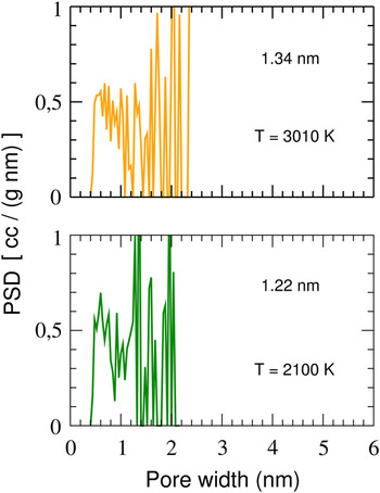
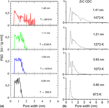
Nanoporous materials are not fully characterized by their SSA and specific pore volume.Reference Linares-Solano, Jordá-Beneyto, Kunowsky, Suárez-García, Cazorla-Amorós, Terzyk, Gauden and Kowalczyk11 The gas adsorption capacities depend also on the size of the pores.Reference Gogotsi, Dash, Yushin, Yildirim, Laudisio and Fischer26 The pore size distribution function (PSDF) gives a detailed characterization of the porous structure of a material. To get meaningful distribution functions from computer simulations, one has to count a sufficiently large number of pores. This requires using very large simulation cells, and for this purpose, we have used cells containing 62,500 carbon atoms, like that shown in Fig. 1. To assign a volume to each pore, we found convenient to model the pores as nonoverlapping spheres. Figures 4 and 5 show the PSDFs obtained for simulation cells of intermediate size (containing 6912 carbon atoms) and large size (containing 62,500 carbon atoms), respectively. The average size and the largest sizes of the pores are smaller in the simulations for the intermediate-size cells, compared to the simulations for larger cells. Moreover, in the simulations for the intermediate-size cells, the PSDF distribution function drops to zero abruptly at the value of the largest pore size. In contrast, the PSDF goes to zero smoothly in the simulations for the large cells. A comparison between the calculated PSDFs (for the large cell) and the experimental PSDFs of CDCs obtained from ZrC precursorsReference Yushin, Dash, Jagiello and Gogotsi19, Reference Gogotsi, Dash, Yushin, Yildirim, Laudisio and Fischer26 is shown in Fig. 5. The average size of the pores increases from 0.94 to 1.40 nm when the simulation temperature increases between 350 and 3010 K, and at the same time, the PSDF distribution becomes broader.Reference López, Cabria and Alonso21 The experiments also indicate an increase of the average pore size, from 0.80 to 1.41 nm, for chlorination temperatures ranging from 873 to 1473 K, and a broadening of the pore size distribution.Reference Gogotsi, Dash, Yushin, Yildirim, Laudisio and Fischer26 As indicated above, the temperature of the theoretical simulations should not be identified with the temperature of the chlorination experiments, but it is clear that the simulations reproduce features of the measured PSDF as the temperature varies. The temperature at which the chlorination experiment is performed determines the most probable pore size, the average pore size, and the pore size distribution.
PSDF of CDCs obtained in MD simulations for intermediate-size supercells (containing 6912 carbon atoms) at two simulation temperatures, 2100 and 3010 K. The initial supercell corresponds to a ZrC precursor. The average size of the pores is shown in each panel.

Comparison between the experimental PSDF of CDCs obtained from ZrC precursorsReference Yushin, Dash, Jagiello and Gogotsi19, Reference Gogotsi, Dash, Yushin, Yildirim, Laudisio and Fischer26 (b) and the PSDF obtained in the computer simulations for large supercells containing 62,500 carbon atoms (a). The average size of the pores is shown in each panel.

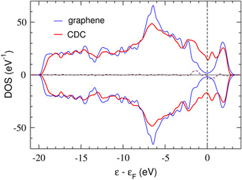
We have also investigated the electronic properties of the ZrC–CDCReference López, Cabria and Alonso21 using the density functional theory (DFT). A cell containing 256 carbon atoms, periodically repeated in space, was used. The structure of the CDC was generated by MD at a temperature of 2100 K using the Tersoff–Nordlund potential,Reference Tersoff22, Reference Nordlund, Keinonen and Mattila25 and it was then reoptimized using DFT. Figure 6 shows the electronic density of states (DOS) of the CDC. The DOS for an infinite graphene layer is included for comparison. Graphene is a zero-gap semiconductor. The CDC develops a band in the energy region around the Fermi level. This band arises from states localized at the edges of the nanographenes forming the pore walls, and these edge states are similar to those reported in graphene nanoribbons.Reference Fujita, Wakabayashi, Nakada and Kusakabe27–Reference Hod, Peralta and Scuseria29 The pore edges in the CDCs are interconnected, and, therefore, the edge states can be considered as delocalized over the sample.
Spin-dependent electronic DOS of the CDC. The dashed line near the horizontal axis is the difference between the spin-up and spin-down DOS. The vertical line indicates the Fermi level. The DOS of graphene is also included. To facilitate the comparison, the DOS of graphene has been duplicated for negative values.

MD simulations of nanoporous carbons have also been performed using a tight-binding methodology, which takes the electronic structure of the system explicitly into account, albeit in an approximate way.Reference Wang, Qiu and Ho30, Reference Peng and Morris31 Because of the increase in the computational effort, the number of carbon atoms in the tight-binding simulations is necessarily smaller than the number of atoms in the simulations that use the Tersoff potential. Wang et al.Reference Wang, Qiu and Ho30 and Peng and MorrisReference Peng and Morris31 have performed simulations with cells containing 512 and 500 carbon atoms, respectively, and they studied the structure of carbons with different densities. Low carbon densities led to porous structures, and the results are consistent with those obtained in the simulations with the Tersoff potential. In summary, computer simulations of the atomistic structure of porous carbons using different descriptions for the interatomic interactions reveal a structure of interconnected pores with graphitized walls containing many defects. The degree of graphitization improves as the annealing temperature increases.
Suarez-Martinez and MarksReference Suarez-Martinez and Marks32 have applied nonequilibrium MD to study the thermal conductivity of noncrystalline carbons with densities in the range 1.4–3.0 g/cm3. The simulations used the environment-dependent interaction potential,Reference Marks33 which reproduces the structure and properties of a variety of carbon allotropes. Amorphous carbon structures were obtained by a liquid-quench method. In those structures, the fraction of atoms with sp 3 bonding (tetrahedral-like coordination) increases linearly with the density of the material, as observed experimentally.Reference Ferrari, Libassi, Tanner, Stolojan, Yuan, Brown, Rodil, Kleinsorge and Robertson34 Investigation of the amorphous carbon with a density 1.5 g/cm3 revealed the emergence of graphite-like structures when that material was annealed at temperatures of 3500–4000 K. The ordering was ascribed to a self-assembling process driven by sp 3 to sp 2conversion.
The structure of amorphous and porous carbons has also been studied using reverse Monte Carlo (RMC) modeling.Reference Thomson and Gubbins35–Reference Zetterström, Urbonaite, Lindberg, Delaplane, Leis and Svensson37 In this method,Reference McGreevy and Putszai38 an initial configuration of atom positions is created. Then, the Monte Carlo method is used to randomly displace the atoms until the calculated pair distribution function and the total structure factor produce a good fit to the pair distribution function and total structure factor determined from small angle x-ray scattering, x-ray diffraction, or neutron diffraction experiments. Constraints on the interatomic C–C distances, atomic coordination, and C–C–C angles are usually imposed during the modeling. The final atomic configurations are very sensitive to those constraints and to the starting configuration. Zetterström et al.Reference Zetterström, Urbonaite, Lindberg, Delaplane, Leis and Svensson37 have performed RMC modeling using neutron powder diffraction data from porous carbons prepared by chemical chlorination of TiC at temperatures between 973 and 1473 K. The starting structures and the constraints were chosen to favor graphitization. One of the starting structures was a model formed by perfect graphitic layers separated by distances from 3.35 to 5.40 Å to obtain a lower density. A different starting structure consisted of defect graphitic layers separated to 3.40 Å. The defects were primarily built by removing carbon atoms. The second starting model led to structure factors in better agreement with experiment. The result of the simulation is that the starting structure of separated layers is maintained, but two tendencies are observed: the first one is the formation of cavities in the layers and the second is the puckering and rearrangements of the carbon atoms within each layer. A hybrid RMC algorithm, which incorporates both experimental and energy-based constraints, has been applied by Opletal et al.Reference Opletal, Petersen, McCulloch, Snook and Yarovsky36 to investigate the microstructure of disordered carbons. The densities of the two studied materials, 2.4 and 3.0 g/cm3, are larger than those typical of porous carbons and correspond to materials containing low and high fractions of atoms with diamond-like bonding, respectively.
III. INTERACTION OF MOLECULAR HYDROGEN WITH CARBON SURFACES
When molecular hydrogen interacts with a graphitized carbon surface without defects, the molecule becomes weakly bound to the carbon layer by a physisorption mechanism. Li et al.Reference Li, Furuta, Goto, Ohashi, Fujiwara and Yip9 have estimated the optimum adsorption enthalpy for the occurrence of reversible adsorption/desorption of hydrogen under the conditions required for automotive applications. They considered the case of hydrogen injected under pressure and used the van’t Hoff equation to study the equilibrium between two phases of hydrogen: one is the condensed phase formed by the hydrogen physisorbed on the surface of the pores and the other phase is formed by the compressed gaseous hydrogen occupying the empty space of the material. The difference in chemical potential, Δμ = Δh − TΔS, where Δh is the change in specific enthalpy between the gas phase and the adsorbed phase of hydrogen and ΔS is the change in specific entropy, controls the direction of adsorption/desorption. The specific enthalpy and entropy are the enthalpy and entropy per hydrogen molecule, respectively. The entropy per molecule in hydrogen gas at room temperature and 1 atm of pressure is close to 15.6 kB.Reference Schroeder39 On the other hand, the entropy in the adsorbed phase is much less. Therefore, to achieve reversible adsorption/desorption near room temperature, Δh should be about 10–15 kBT/molecule, which amounts to an adsorption enthalpy of about 0.30 eV per H2 molecule. Another requirement is that Δh should depend weakly on the hydrogen coverage X. This arises because hydrogen should stay adsorbed to near saturation up to temperatures near 330 K but should be totally desorbed at T = 400 K, which is the upper temperature limit provided by the fuel cell heat recycling system. This will occur if Δh(X) varies from 0.30 to 0.40 eV/molecule when X varies from saturation to zero. Another thermodynamic estimation has been given by Bhatia and Myers.Reference Bhatia and Myers10 For adsorption and desorption pressures of 30 and 1.5 bar, respectively, at 298 K, they estimate an optimum Δh of 0.16 eV/molecule.
In Sec. II, we have seen that the walls of the pores in the CDCs show a high degree of graphitization. For this reason, it is relevant to calculate the adsorption energy of molecular hydrogen on planar and curved graphene. The adsorption of H2 on a planar graphene layer has been studiedReference Arellano, Molina, Rubio and Alonso40–Reference Cabria, López and Alonso42 using the DFT formalism.Reference Kohn and Sham43, Reference Parr and Yang44 The adsorption energy is defined:
 $$E_{{\rm{ads}}} \, = \,E({\rm{H}}_2 )\, + E({\rm{graphene}}) - E({\rm{H}}_2 \,{\rm{on}}\,{\rm{graphene}})\quad,$$
where E(H2) is the energy of the hydrogen molecule, E(graphene) is the energy of the graphene layer, and E(H2 on graphene) is the energy of the system formed by the molecule adsorbed on the graphene layer. Adsorption energies, calculated for different positions and orientations of the adsorbed molecule using the local density approximation (LDA) to electronic exchange and correlation effects,Reference Kohn and Sham43, Reference Parr and Yang44 vary between 0.07 and 0.09 eV per molecule.Reference Arellano, Molina, Rubio and Alonso40, Reference Cabria, López and Alonso42 These values are in the physisorption range, in which the molecule interacts weakly with the graphitic layer. The most stable position is above the center of a carbon hexagon, and the configuration with the molecular axis parallel to the layer is slightly more favorable than the perpendicular orientation. The LDA adsorption energies are in reasonable agreement with the results of second-order Möller–Plesset (MP2) perturbation calculations: Okamoto and MiyamotoReference Okamoto and Miyamoto41 and Ferre-VilaplanaReference Ferre-Vilaplana45 obtained adsorption energies of 0.086 and 0.064 eV, respectively. In contrast, the generalized gradient approximations, GGA, give a repulsive interaction and do not predict binding. Experiments for the adsorption of H2 on the surface of graphiteReference Mattera, Rosatelli, Salvo, Tommasini, Valbusa and Vidali46 measured an adsorption energy value of 0.042 eV. Correcting the theoretical adsorption energy by subtracting the zero-point energy for the motion of the molecule in the adsorption potential well improves the predictions. For instance, the zero-point energy of the molecule in the LDA interaction potential well is about 0.015 eV, and this gives corrected LDA binding energies between 0.055 and 0.075 eV/molecule. To avoid confusion, one should notice that this zero-point energy has nothing to do with the zero-point energy for the internal vibrational energy of the molecule.
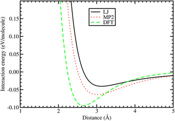
Three calculated interaction potential curves of a hydrogen molecule with a graphene layer are shown in Fig. 7. The wall of the potential at short separation is due to the repulsive interaction, which develops when the closed electronic shell of the hydrogen molecule overlaps substantially with the electron density of the substrate. The density functional (DFT-LDA) potentialReference Cabria, López and Alonso47, Reference Cabria, López and Alonso48 captures the weak interaction between the molecule and the graphene layer, although overestimating its strength. The binding obtained in the LDA calculation is mainly due to electronic exchange and correlation effects. The LDA exchange energy functional is given as:
 $$E_x^{{\rm{LDA}}} [{\rm{\rho }}] = \int {{3 \over 4}\left( {{3 \over {\rm{\pi }}}} \right)^{\!1/3} {\rm{\rho }}(\vec r)^{4/3} d^3 r}\quad ,$$
LJ, MP2, and density functional (DFT-LDA) interaction potentials between a hydrogen molecule and a planar graphene layer. In the case of MP2, the graphene layer was simulated by a planar C24H12coronene.

where  ${\rm{\rho }}(\vec r)$ is the electron density of the system. Correlation is not considered in this discussion only for the purposes of simplicity, but it is included in the calculations. The exchange energy density
 $e_x ({\rm{\rho }}(\vec r)) = 3/4(3/{\rm{\pi }})^{1/3} {\rm{\rho }}(\vec r)^{4/3}$ is nonlinear in the electron density. As a consequence of the nonlinearity, there is a bonding contribution between the hydrogen molecule and the graphene layer for weakly overlapping electron densities, even in the absence of any relaxation of the density. In addition, the small relaxation of the electron density also contributes to the binding.Reference Arellano, Molina, Rubio and Alonso40 On the other hand, the LDA potential goes to zero too fast at large separations because it does not include dispersion forces, responsible for the long-range van der Waals interaction. The van der Waals forces can be viewed as arising from nonlocal electronic correlations.Reference Alonso and Mañanes49
The Lennard-Jones (L-J) potential:
 $$U(r)\, = \,4{\rm{\varepsilon }}\left[ {\left( {{{\rm{\sigma }} \over r}} \right)^{12} - \left( {{{\rm{\sigma }} \over r}} \right)^6 } \right]\quad,$$
where r is the distance between the center of mass of the hydrogen molecule and the carbon atom, and ε and σ are constants to be fitted, was used by Bhatia and Myers.Reference Bhatia and Myers10 This potential gives, by construction, the correct behavior at long distances because it contains an attractive 1/r 6 term, but Fig. 7 shows that it yields an interaction at equilibrium that is too weak compared to the other two potentials. The strength and equilibrium distance of the MP2 interaction, which provides a reliable account of the dispersion forces, are intermediate between those of the LJ and the DFT-LDA potentials. The MP2 adsorption energy, E ad, amounts to 0.064 eV/molecule. In those MP2 calculations,Reference Ferre-Vilaplana45 the graphene layer was simulated by a planar C24H12 molecule with the dangling bonds at the perimeter saturated by hydrogen atoms. The experimental depth of the potential well has been estimated by Mattera et al.Reference Mattera, Rosatelli, Salvo, Tommasini, Valbusa and Vidali46 by fitting an empirical potential that reproduces their experimental results for the adsorption of H2 on the graphite surface. The depth of that potential is 0.052 eV. The MP2 interaction potential is then more accurate than the other two. To close the discussion on the adsorption energy of H2 on planar graphitic surfaces, we mention a recent workReference Carrete, Longo, Gallego, Vega and Balbás50 in which the adsorption energy of H2 on graphene nanoribbons was calculated using DFT with new exchange–correlation functionalsReference Dion, Rydberg, Schröder, Langreth and Lundqvist51, Reference Klimes, Bowler and Michaelides52 adapted to account for the van der Waals interactions. The conclusion was that the adsorption energies of H2 calculated with the LDA and with the nonlocal functionals including the van der Waals interactions are very close. Our interpretation of this unexpected result is that the region of the interaction potential near the minimum is dominated by exchange and correlation effects described reasonably well by the LDA. Of course, the correct 1/r 6tail is only accounted for by the nonlocal van der Waals functionals.
It is clear from the experimental and theoretical work discussed above that the strength of the adsorption energy of molecular hydrogen on a graphitic surface is below 0.10 eV/molecule. LDA calculations for H2 adsorbed on the outer wall of carbon nanotubes led to the same conclusion,Reference Arellano, Molina, Rubio, López and Alonso53, Reference Cabria, López and Alonso54 and an experimental estimation by Brown et al.Reference Brown, Yildirim, Newmann, Heben, Gennett, Dillon, Alleman and Fischer55 gave 0.062 eV/molecule. The adsorption energies fall short of the values required for reversible adsorption/desorption near room temperature and moderate pressures. These small adsorption energies explain why the measured hydrogen storage capacities of pure carbon nanotubes at room temperature are less than 1 wt%Reference Züttel56 (one should notice that, in the experiments, hydrogen is mostly adsorbed on the outer surface of the nanotubes because the ends of many nanotubes are closed).
The adsorption energies of H2 are enhanced when the molecules are confined in cavities between two closely spaced parallel surfaces or near a concave surface of large curvature. This situation occurs in nanoporous materials.Reference Yushin, Dash, Jagiello and Gogotsi19, Reference Gogotsi, Dash, Yushin, Yildirim, Laudisio and Fischer26, Reference Jorda–Beneyto, Suarez–García, Lozano–Castelló, Cazorla–Amorós and Linares-Solano57, Reference Cabria, López and Alonso58 A slit pore, which consists in two parallel graphene layers separated by a distance d, has been often used to model the pores present in nanoporous carbons and to analyze the measured gas adsorption properties. The minimum of the H2–graphene interaction potential shown in Fig. 7 occurs for a distance from the layer close to 3 Å, so in a slit pore having a width d of about 6 Å, the hydrogen molecule would interact at the same time with the two parallel graphene surfaces, increasing the adsorption binding energy by about a factor of two. The adsorption energy also increases inside a curved nanopore: the adsorption energies inside (6,6) and (5,5) carbon nanotubes obtained in DFT-LDA calculations are 0.12 and 0.17 eV/molecule, respectively.Reference Arellano, Molina, Rubio, López and Alonso53 The diameters of those two nanotubes are d(6,6) = 8.23 Å and d(5,5) = 6.81 Å. These values of the adsorption energy should be compared with the adsorption energy on the outer surface of any of the tubes, 0.07 eV/molecule.Reference Arellano, Molina, Rubio, López and Alonso53 The adsorption inside a pore having the form of a bowl has also been studied.Reference Cabria, López and Alonso58 That pore was modeled by a short (7,7) nanotube open at one end and capped at the other end by a semispherical half-fullerene, C52, which has a diameter similar to that of the nanotube. The DFT-LDA adsorption energy inside that pore reaches the value E ads= 0.2 eV/molecule.
IV. HYDROGEN STORAGE IN POROUS CARBONS
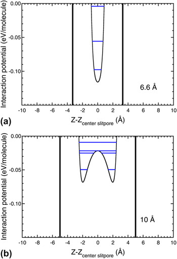
The predictions of enhanced hydrogen adsorption energies in carbon pores have motivated calculations of the storage capacities of nanoporous carbons. For this purpose, simplified models have been used for the shape of the pores, and the simplest model is a slit pore. A thermodynamic model has been applied to calculate the storage capacities of graphene slit pores. The amount of hydrogen stored in the pores at a given temperature T is determined by the thermodynamic equilibrium between a condensed hydrogen phase, formed by the hydrogen adsorbed on the pore walls, and a nonadsorbed compressed gas phase introduced in the material by applying an external pressure P ext. The thermodynamic model,Reference Cabria, López and Alonso47, Reference Cabria, López and Alonso48, Reference Patchkovskii, Tse, Yurchenko, Zhechkov, Heine and Seifert59 briefly described next, takes into account the quantum motion of the molecules confined in the volume of the pore. Figure 8 shows the potential experienced by the hydrogen molecules inside pores of width d equal to 6.6 and 10 Å. This potential is evaluated as U(z) = U 1(z) + U 2(d − z), where U 1(z) and U 2(d − z) represent the interaction of the molecule with the left side and right side graphene walls, respectively (the origin of coordinates, z = 0, has been taken on the left-hand side wall of the pore). The MP2 potential of Fig. 7 has been taken for the molecule–graphene interaction. Two separated minima appear in the pore with d = 10 Å, while only one, deeper minimum, appears for the thinner pore of with d = 6.6 Å. The size distribution of pores of nanoporous materials is obtained, in most cases, by deconvolution of the experimental gas adsorption isothermsReference Dash, Yushin and Gogotsi12 using a nonlocal DFT methodReference Tarazona, Marconi and Evans60, Reference Jagiello and Olivier61 in which the pores are modeled as planar pores (slit pores) and the pore width is defined as the distance between the surface planes of the opposite walls. This definition is consistent with the definition of the pore width d that we use throughout this paper.
MP2 interaction potential confining the hydrogen molecules in slit pores of width d = 6.6 Å (a) and d = 10 Å (b). Vertical lines represent the pore walls. Horizontal lines indicate the energies of the quantum states of the molecule in the potential.

As a first step, the quantum states for the motion of the hydrogen molecules confined in the pores are calculated by solving the time-independent Schrödinger equation. The horizontal lines drawn in Fig. 8 represent the quantum states for the molecules in the pore potential U(r). The energy eigenvalues εi of the quantum states are used to evaluate the partition function of the adsorbed phase of hydrogen,  $Z_{{\rm{ads}}} \, = \,\sum\nolimits_i {e^{ - {\rm{\varepsilon }}_i /kT} }$, where k is Boltzmann’s constant and T is the temperature. The model takes into account all the quantum states, but in practice, only two or three deepest states contribute to the partition function. The corresponding partition function of a gas of nonadsorbed compressed (free) molecules confined in the volume of the pore is
 $Z_{{\rm{free}}} \, = \,(d - 2d_{{\rm{excl}}} )\sqrt {2{\rm{\pi }}mkT/h^2 }$, where h is the Planck’s constant. The quantity d excl is an exclusion distance, clearly appreciated in Fig. 8, accounting for the steep repulsion of the interaction potential near to the pore walls. The amount of adsorbed hydrogen at a given temperature T is determined by the thermodynamic equilibrium between the adsorbed hydrogen phase and the free compressed gas phase. The ratio K eq = Z ads/Z free gives the equilibrium constant between the adsorbed and the compressed phases. Then, K eq allows to relate the applied external pressure P ext and the pressure of the adsorbed phase, also called internal pressure, P int, through the van’t Hoff equation:
 $$K_{{\rm{eq}}} \, = \,e^{{1 \over {RT}}\int_{P_{{\rm{ext}}} }^{P_{{\mathop{\rm int}} } } {V_{{\rm{molar}}} (P,T){\rm{ }}dP} } \quad,$$
where R is the gas constant. The molar volume V molar(P,T), which is a key ingredient in this equation, is obtained by the equation of state, EOS, of hydrogen. Based on two previous EOSs for hydrogen fitted by Mills et al.Reference Mills, Liebenberg, Bronson and Schmidt62 and by Younglove,Reference Younglove63 we have built an accurate parameterization of the EOS,Reference Cabria, López and Alonso47, Reference Cabria, López and Alonso48 valid in a broad region of temperatures, 77–300 K, and pressures, 0.005–1500 MPa. From Eq. (7), one obtains the internal pressure P int for given values of the external pressure P ext and T, and then, from the EOS, we find the molar volume of the adsorbed hydrogen phase, V molar(P int,T). The stored hydrogen is composed of two phases, the phase corresponding to adsorbed hydrogen and the phase corresponding to compressed gas. The relevant storage capacities are the excess storage capacities, due to the adsorbed phase only.
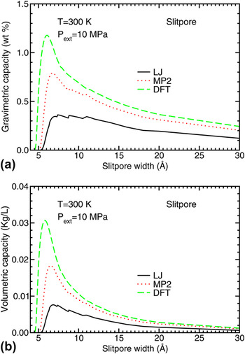
Figure 9 shows the predicted gravimetric and volumetric hydrogen storage capacities of an ideal porous carbon material formed by slit pores of equal width, calculated for an external pressure of 10 MPa and a temperature T = 300 K. Results are compared for the three potentials, LJ, MP2, and DFT, as a function of the pore width. The qualitative behavior of the storage capacity curves is the same: the curves show a maximum for widths between 6 and 7 Å, giving the optimum width of the pores. However, there are substantial quantitative differences in the amount of hydrogen stored. There is a correlation between the storage capacities in Fig. 9 and the depth of the DFT, MP2, and LJ potential wells in Fig. 7: the LJ storage capacities are lower than the MP2 capacities, and these are lower than the DFT capacities. The optimal pore sizes are consistent with experiments and previous theoretical results. By performing grand canonical Monte Carlo simulations of the storage of molecular hydrogen at 300 K and 10 MPa, Rzepka et al.Reference Rzepka, Lamp and de la Casa-Lillo64 predicted optimal hydrogen storage in slit pores of width d optimum ≈ 7 Å. De la Casa-Lillo et al.Reference de la Casa-Lillo, Lamari-Darkrim, Cazorla-Amorós and Linares-Solano65 measured the volumetric hydrogen storage capacities of ACs and AC fibers at 293 K and 70 MPa. Assuming the pores to be slit pores, they reported an optimal pore width d optimum= 6.6 Å.
Excess gravimetric (a) and volumetric (b) hydrogen storage capacities of planar pores, as a function of the pore width, obtained using LJ, MP2, and DFT potentials. The results correspond to temperature T = 300 K and external pressure of 10 MPa.

The calculated hydrogen storage capacities shown in Fig. 9 fall below the DOE target. For instance, at the optimized pore sizes, the gravimetric capacity w(MP2) is equal to 0.8 wt%, and the volumetric capacity C V is 0.018 kg/L, to be compared with the target values of 5.5 wt% and 0.040 kg of hydrogen per liter, respectively. The hydrogen storage capacities are substantially enhanced at low temperature.Reference Cabria, López and Alonso48 At 77 K, the optimum slit pore width increases to 9–10 Å, and the gravimetric capacity reaches values of more than 3 wt%. Interestingly, the value of 0.06 kg/L predicted for the volumetric storage capacity C V at 77 K fulfills the DOE objective. But such low temperatures are of no practical interest for onboard automotive applications, except perhaps in outer space vehicles. In the storage model used here, each graphene wall is part of a single pore. In a previous work,Reference Cabria, López and Alonso47 we assumed that each planar wall was part of two adjacent slit pores. That increases the gravimetric storage capacity by a factor of 2. The situation in real materials is, probably, in between. In fact, as we have discussed in Sec. II, our MD simulations of the CDCs indicate that 50% of the pore walls expose their two sides to gas adsorption and another 50% expose only one side. This gives a factor of 1.5.
As discussed at the beginning of this section, the model we have used for calculating the gravimetric and volumetric hydrogen storage capacities combines Boltzmann statistics with a quantum treatment of the confinement of the hydrogen molecules in the pores. The role of statistics on the adsorption and storage of molecular hydrogen in model carbon foams has been explored by Martínez-Mesa et al.Reference Martínez-Mesa, Yurchenko, Patchkovskii, Heine and Seifert66 For the range of temperatures considered, 50–300 K, the use of Boltzmann or Bose–Einstein statistics gave the same results: the adsorption isotherms calculated using the Bose–Einstein or the Maxwell–Boltzmann statistics remain indistinguishable in the whole pressure range. In fact, it is well known that the Bose–Einstein statistics plays a minor role in quantum fluids at temperatures above 20 K and at typical condensed phase densities.Reference McCoy, Rick and Haymet67, Reference Rick, McCoy and Haymet68
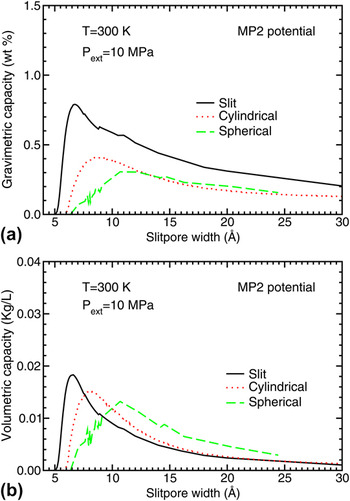
The simple shape of the planar slit pores is convenient both to perform theoretical simulations of the hydrogen storage and as a model to analyze the experimental measurements. However, the simulations presented in Sec. II show that pores in carbon materials can also have other shapes resembling cylindrical or near spherical pores. Theoretical studies of the hydrogen storage in those pores have been performed.Reference Cabria, López and Alonso48, Reference Cabria, López and Alonso58Figure 10 shows a comparison of the predicted storage capacities of planar, cylindrical, and spherical pores at 300 K and a pressure of 10 MPa obtained from MP2 potentials. The storage capacities have been plotted as a function of the pore width: the distance d between the two graphene layers in the case of slit pores and the diameter in cylindrical and spherical pores. The pores present optimal widths, which maximize the hydrogen storage, and the largest storage capacities occur for the planar slit pores.
Excess gravimetric (a) and volumetric (b) hydrogen storage capacities of planar, cylindrical, and spherical pores as a function of the pore size, obtained using the MP2 potential. The results correspond to temperature T = 300 K and external pressure of 10 MPa.

Peng and MorrisReference Peng and Morris20, Reference Peng and Morris31 have performed computer simulations of the hydrogen storage using realistic models of porous carbons. Instead of assuming idealized forms for the pores, they generated porous carbon structures by MD simulationsReference Peng and Morris20 using the Tersoff potentialReference Tersoff22 (see Sec. II above). Two analytical forms were explored for the interaction between the hydrogen molecule and the carbon atoms of the pores. One is the LJ potential of Eq. (6), with ε = 3.69 meV/molecule (0.356 kJ/mol) and σ = 2.97 Å. The other potential has the formReference Patchkovskii, Tse, Yurchenko, Zhechkov, Heine and Seifert59:
 $$U(r)\, = \,Ae^{ - {\rm{\alpha }}r} + C_6 r^{ - 6} \quad,$$
with A = 1099.52 eV/molecule, C 6 = −17.3640 eV Å6/molecule, and α = 3.5763 Å−1. For equilibrium adsorption, the chemical potential of the compressed free gas has to be equal to that of the adsorbed gas. Using this equilibrium condition, Peng and Morris obtained an equation for the effective internal pressure P int (the pressure of the adsorbed phase) as a function of the external pressure P ext (the pressure measured in the laboratory; equal to the pressure of the compressed phase) and the adsorption energy E ads:
 $$P_{{\rm{int}}} \, = \,P_{{\rm{ext}}} e^{ - E_{{\rm{ads}}} /k_{\rm{B}} T}\quad .$$
This equation shows that the internal pressure is a local quantity, which varies with the position of the hydrogen molecules in the porous material because the local adsorption energy changes with the surrounding carbon environment. The local density of adsorbed molecules is related to the local internal pressure and the temperature through the EOS of hydrogen, and the empirical EOS of Mills et al.Reference Mills, Liebenberg, Bronson and Schmidt62 was used for this purpose. Then, the total amount of adsorbed hydrogen was calculated by integrating the local density of adsorbed hydrogen molecules over the structure of the material. The result was that those porous carbons can store up to 0.5 wt% hydrogen at 298 K and 5 MPa, in good agreement with the measurements for ACs under the same temperature and pressure conditions.Reference Jorda–Beneyto, Suarez–García, Lozano–Castelló, Cazorla–Amorós and Linares-Solano57
More recently, Peng and MorrisReference Peng and Morris31 have used the same thermodynamic model to study the hydrogen storage capacity of the porous carbon model materials generated by the tight-binding methodology (see Sec. II). The computer simulations confirm that hydrogen molecules aggregate in narrow pores. This conclusion is consistent with the results of small angle neutron scattering studies of hydrogen adsorption on ACs.Reference Gallego, He, Saha, Contescu and Melnichenko69 The density of adsorbed hydrogen measured in those experiments was approaching the density of liquid H2. The experiments also indicated that the gas densification was larger in the narrow pores. The simulations show that the gravimetric hydrogen storage capacity and the available adsorption volume decrease as the density of the porous carbon material increases. This feature is easy to understand: a higher density of the porous carbon yields less porosity. The calculated excess gas uptake at a temperature of 298 K and a pressure of 5 MPa has a maximum value of 1.33 wt% at a carbon bulk density of 0.8 g/cm3. This value is much higher than the gas uptake predicted by the same authors using the porous carbon models generated with the Tersoff potential: a maximum of 0.5 wt% of hydrogen under the same conditions of temperature and pressure. The total hydrogen uptake is correlated with the available nanopore volume of the material. All pores in the simulated carbons are nanopores, very effective in storing hydrogen. Consequently, an increase of the volume fraction of nanopores leads to an increase of the total gas uptake.
The computer simulations indicate that the pores have some open edges, with carbon showing atomic coordination of two. The edges are reactive, and its effect on hydrogen adsorption has been studiedReference Bores, Cabria, Alonso and López70 using DFT. Carbon nanoribbons with zigzag and armchair edge terminations were considered. Molecular hydrogen dissociates and adsorbs atomically at the nanoribbon edges with no barriers or small activation barriers. The adsorption energies per hydrogen molecule are quite large, 2.5 and 5.7 eV for armchair and zigzag edges, respectively. This indicates that the open edges are very reactive and will be saturated with hydrogen or any other molecule whenever available. However, under mild conditions of pressure and temperature, hydrogen cannot be desorbed from the edges, and, therefore, the edges do not contribute to the reversible storage capacity of the material.
V. ENHANCEMENT OF HYDROGEN STORAGE BY DOPING POROUS CARBONS
From the discussion in Sec. IV, we know that hydrogen storage on clean porous carbons at room temperature and moderate pressures does not fulfill the DOE targets. Doping the carbon materials with metallic impurities represents a promising strategy to enhance the hydrogen uptake. The metallic atoms have the effect of increasing the binding energies of molecular hydrogen to the nanopore walls. In addition, the deposited metallic atoms absorb several H2 molecules.Reference Kiran, Kandalam and Jena71–Reference Yildirim and Ciraci74 An increase of the hydrogen storage capacities of carbon nanotubes doped with lithium and potassium, as compared to clean nanotubes, has been observed.Reference Chen, Wu, Lin and Tan75, Reference Yang76 The atypical hydrogen uptake observed by Bath et al.Reference Bath, Contescu, Gallego and Baker77 on chemically activated microporous carbon has been proposed to be due to traces of alkali metals residual from the process of chemical activation.
The most stable position of a Li atom adsorbed on a graphene layer is a hollow site above the center of a carbon hexagon. The Li atom transfers a charge of 0.5–0.6 e to grapheneReference Cabria, López and Alonso42, Reference Khantha, Cordero, Molina, Alonso and Girifalco78, Reference Zhu and Lu79 and becomes partially ionized. Most of this charge concentrates in the region between the Li atom and the carbon layer. The adsorption energy of the Li atom in DFT calculations is close to 1 eV, and the equilibrium distance between the Li atom and the carbon layer is 1.7–1.8 Å.Reference Cabria, López and Alonso42, Reference Chan, Neaton and Cohen80 The interaction between Li and graphene is partly ionic and partly covalent. Cabria et al.Reference Cabria, López and Alonso42 and Cho and ParkReference Cho and Park81 have performed DFT calculations, with the LDA and GGA, respectively, comparing the adsorption of H2on pure and Li-doped graphene and carbon nanotubes. The adsorption energy of molecular hydrogen on doped graphene is defined as:
 $$E_{{\rm{ads - doped}}} \, = \,\,E({\rm{H}}_2 ) + E({\rm{Li - doped \;graphene}}) - E({\rm{H}}_2 \,{\rm{on \;Li - doped \;graphene}})\quad.$$
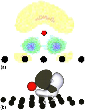
The adsorption energies of H2 are enhanced substantially by the presence of lithium, reaching values of 0.17–0.20 eV per H2 molecule. The increase with respect to the adsorption of H2 on clean graphene amounts to a factor of two. A similar increase occurs in DFT calculations for the adsorption on fullerenes and nanotubes doped with lithiumReference Cabria, López and Alonso42, Reference Zhu and Lu79, Reference Sun, Jena, Wang and Marquez82 and potassium.Reference Froudakis83 The increase of the H2 adsorption energy is due to the polarization of the charge of the hydrogen molecule by the neighbor charged alkali atoms. The first panel of Fig. 11 shows the electron density redistribution Δρ when a Li atom is absorbed on the graphene layer:
 $$\Delta {\rm{\rho }}\, = \,{\rm{\rho }}({\rm{graphene}} + {\rm{Li}}) - \,{\rm{\rho }}({\rm{graphene}}) - \,{\rm{\rho }}({\rm{Li}})\quad.$$
(a) Electron density redistribution Δρ = ρ(graphene + Li) − ρ(graphene) − ρ(Li), when a Li atom is absorbed on a graphene layer. Electronic charge is lost in the light-colored region above the Li atom (negative Δρ). This charge is transferred to the region between the atom and the carbon layer. (b) Polarization of the charge of the adsorbed hydrogen molecule due to the presence of an adsorbed Li atom nearby. Black and white regions indicate excess and defect of electronic charge, respectively, compared to a free H2molecule. In the two panels, the position of the Li atom is indicated by the small red sphere.

The light-colored region above the Li atom represents a loss of electron density (negative Δρ). This charge is transferred to the region in between the atom and the carbon layer. The second panel shows the polarization of the charge of the hydrogen molecule due to the nearby presence of a charged Li atom.
Assuming that Li doping leads to a similar increase, by a factor of two, in the depth of the MP2 interaction potential between H2 and graphene, the depth of this potential can be estimated as 0.12–0.13 eV. We can then make a rough quantitative estimate of the effect of Li doping on the hydrogen storage capacity. It has been mentioned in Sec. IV that the calculated maximum storage capacities of Fig. 9 correlate well with the depth of the interaction potentials of Fig. 7. This correlation is nearly linear. Using that correlation, we find that the new MP2 H2–graphene interaction potential, corrected by the effect of lithium doping, predicts gravimetric storage capacities close to 1.5 wt% in slit pores. This value may increase to about 2% if we allow for the fact that many carbon walls may form part of two adjacent pores. The combined effect of doping and confinement in narrow pores has been analyzed. LDA calculations for the adsorption of H2 inside a Li-doped pore, with the pore having a bowl-like shape modeled as a short (7,7) nanotube open at one end and closed on the other end by a semispherical carbon cage, yield adsorption energies in the range 0.28–0.33 eV per H2 molecule.Reference Cabria, López and Alonso58 Although perhaps a bit overestimated due to the use of the LDA in the calculation, these values for the adsorption energy are very encouraging and give support to the beneficial effect of metal doping. The investigation of the possible reactions of Li with molecular hydrogen producing lithium hydride, LiH, or with residual moisture yielding LiOH, are out of the scope of this paper and have not been considered here. Those reactions could poison the alkaline dopant reducing its beneficial effect on the storage capacity of the material.
The effect of doping with alkaline earth atoms and transition metal atoms has also been explored.Reference Kiran, Kandalam and Jena71–Reference Yildirim and Ciraci74, Reference Yoon, Yang, Hicke, Wang, Geohegan and Zhang84–Reference Contescu, van Benthem, Li, Bonifacio, Pennycook, Jena and Gallego89 Again, the calculations show that the presence of the metallic impurities increases the strength of the adsorption binding energy of H2 on graphitic-like surfaces. Aggregation of adsorbed dopant atoms to form three-dimensional clusters may occur at high coverage if the attractive interactions between metal atoms are larger than the adsorption energy of the dopant atom on graphene. The clustering of Pd atoms on the surface of graphene,Reference Cabria, López and Alonso90 Ti atoms on the surface of fullerenes,Reference Sun, Wang, Jena and Kawazoe86 and Sc atoms on the surface of nanotubesReference Krasnov, Ding, Singh and Yakobson91 has been studied in detail. Clustering of the dopant atoms should be avoided if possible. In their experiments, Contescu et al.Reference Contescu, van Benthem, Li, Bonifacio, Pennycook, Jena and Gallego89 observed that 18% of the Pd deposited on porous carbons was in atomic form and the rest in the form of clusters and nanoparticles. Clustering will be avoided if the metal atoms occupy substitutional positions in the two-dimensional graphene lattice.Reference Krasheninnikov, Lehtinen, Foster, Pyykkö and Nieminen92 The calculations of Sigal et al.Reference Sigal, Rojas and Leiva93 have shown that oxygen interferes with hydrogen adsorption in the doped carbons, by either blocking the adsorption sites or by the oxidation of the metal atoms and particles. Consequently, it is necessary to reduce the oxygen partial pressures sufficiently to allow for hydrogen storage.
On the other hand, the supported metallic clusters may act as a catalyst that enhances the hydrogen uptake of carbon substrates through the mechanism of spillover.Reference Lueking and Yang94–Reference Lachawiec, Qi and Yang97 Conner and FalconerReference Conner and Falconer98 defined the concept of spillover as the transport of a molecule adsorbed on a first surface onto a second surface that does not adsorb the molecule under the same conditions. Transition metals, in particular Ni, Pd, and Pt, which are in the same column in the periodic table, are good catalysts to induce the spillover of hydrogen on graphitic materials. Yakobson et al.Reference Singh, Ribas and Yakobson99 have performed simulations of the hydrogen spillover induced by a Pd4 cluster supported on graphene. When the adsorption of hydrogen on the Pd4cluster reaches saturation, hydrogen can spillover the carbon receptor. The presence of a phase of hydrogenated graphene facilitates the spillover, but the spillover on a pristine graphene surface is not energetically favorable.
VI. CONCLUSIONS
Achieving an efficient storage of hydrogen is a key step in the technological program that would lead to the use of hydrogen as a fuel in the cars of the future. Those cars will use hydrogen fuel cells instead of electric batteries or gasoline engines, only releasing water as a waste product. Nanoporous carbons are listed between the most promising materials for storing hydrogen, adsorbed on the inner surfaces of the pores. Because of their porous structure, these materials have a very large SSA, of several thousand m2/g. The structure of porous carbons at an atomic scale is not well characterized, and we have investigated the structure of carbide-derived porous carbons. The computer simulations show that the CDCs exhibit a structure of interconnected pores of nanometric size, with graphitic-like walls.
We have used a quantum thermodynamic model and H2–carbon wall interaction potentials derived from theoretical and empirical approaches to study the storage of hydrogen in carbon materials with pores of different shapes. The predicted storage capacity of porous carbons is sizable at cryogenic temperatures, but at room temperature, the storage falls below the DOE targets. This indicates that just an optimization of the pore shapes and sizes is not enough to reach the targets. The failure is a consequence of an insufficiently strong attractive interaction between the hydrogen molecule and the pore walls. Recent work indicates that doping the carbon material with metallic impurities leads to the enhancement of the binding energy of H2to the pore walls. Consequently, metallic doping may provide a route to increase the hydrogen storage capacity of porous carbons.
ACKNOWLEDGMENTS
Work supported by MICINN of Spain and the European Regional Development Fund (Grant No. MAT2011-22781) and by Junta de Castilla y León (Grant No. VA158A11-2).