

1. Introduction
Rate equations are essential for describing biological processes. Numerous experimental studies, as exemplified by those on enzyme catalysis and protein folding, involve the measurement of rate constants by fitting to phenomenological rate equations. However, to interpret such results on rate constants requires some understanding of how rate constants are related to the microscopic behaviors of the systems under study. Deriving rate constants from microscopic descriptions is the goal of rate theories. Among the rate theories that are most widely applied to biological systems today are those by Eyring (Reference Eyring1935), Kramers (Reference Kramers1940), and Smoluchowski (Reference Smoluchowski1917). These theories are based on fundamental principles of statistical mechanics, and, remarkably, were inspired by systems far simpler than biomacromolecules. More modern theories have extended this early work in many directions (e.g., Agmon & Hopfield, Reference Agmon and Hopfield1983; Grote & Hynes, Reference Grote and Hynes1980; Melnikov & Meshkov, Reference Melnikov and Meshkov1986; Solc & Stockmayer, Reference Solc and Stockmayer1973; Szabo et al. Reference Szabo, Schulten and Schulten1980; Zhou, Reference Zhou1993). Unfortunately, the newer developments are not accessible to many experimentalists.
It is clear that a basic understanding of rate theories is useful for interpreting measured rate constants and for gaining molecular insight into biological processes. This paper aims to introduce the central ideas of some of the most important rate theories. It is hoped that, by delving into some of the details and subtleties in the development of the theories, the paper will help the reader gain a more than superficial perspective. Several examples are presented to illustrate how rate theories can be used to yield microscopic knowledge on biomolecular behaviors. There is growing interest in how the crowded environments inside cells affect the kinetic properties of biomolecules (Zhou et al. Reference Zhou, Rivas and Minton2008). We will outline how the effects of macromolecular crowding can be accounted for in calculating rate constants.
We also attempt to clear up a number of misconceptions in the literature regarding popular rate theories. For example, it is often stated that the pre-exponential factor of the rate constant predicted by the transition-state theory is k BT/h, where k B is Boltzmann's constant, T is the absolute temperature and h is Planck's constant. Such a misstatement would suggest that quantum effects are prevalent in rate processes. In addition, Smoluchowski's result for diffusion-controlled non-specific binding of spherical particles is often quoted as providing an upper bound for the rate constants of stereospecific protein–ligand or protein–protein binding. In fact, because of the orientational constraints arising from the stereospecificity, the rate constant limited by random diffusion is several orders of magnitude lower than the Smoluchowski result.
It has been recognized that rate constants, as opposed to equilibrium constants, are of paramount importance in many biological processes (Schreiber et al. Reference Schreiber, Haran and Zhou2009; Zhou, Reference Zhou2005a). A focus of systems biology nowadays is on rate constants of steps comprising various networks; it has been demonstrated, through mutations, that the protein association rate constant in one step can dictate the overall activity of a signaling network (Kiel & Serrano, Reference Kiel and Serrano2009). When several ligands compete for the same protein or when one protein is faced with alternative pathways, kinetic control, not thermodynamic control, dominates in many cases; this is especially true when dissociation is slow (see Fig. 1). In particular, during protein translation, cognate and non-cognate aminoacyl-tRNAs all compete to bind to the decoding center on the ribosome. Understanding how rate constants are regulated is crucial for elucidating mechanisms of biological processes.
Thermodynamic control versus kinetic control. A protein in state A has two reaction pathways, leading to states B1 and B2, respectively. The forward and reverse rate constants of the two pathways are k ±1 and k ±2. Three of the constants are fixed: k +1=10 s−1, k +2=0·1 s−1, and k −1=0·01 s−1. The ratio, k +1/k +2, of the two forward rate constants is thus fixed at 100. The fourth rate constant, k −2, is varied from10−4 to 10−8 s−1, yielding the five values for the ratio of the two equilibrium constants shown in the figure. The equilibrium concentration of B1 is [B1]eq=C tk +1k −2/(k +1k −2+k +2k −1+k −1k −2), where C t is the total protein concentration; [B2]eq is obtained by reversing the indices 1 and 2. With the protein is initially in state A, the time dependence of the B1 concentration is given by

where λ±=[k +1+k −1+k +2+k −2±((k +1+k −1−k +2−k −2)2+4k +1k +2)1/2]/2. Again [B2] is obtained by reversing the indices 1 and 2. Thermodynamic control means [B1]/[B2]→[B1]eq/[B2]eq, indicated by the arrows on the right, whereas kinetic control means [B1]/[B2]→k +1/k +2, indicated by the arrow at the top. Note that the two pathways can represent either unimolecular or bimolecular reactions. An example of the latter case is a protein binding with two different ligands; k +1 (or k +2) is then a pseudo-first-order rate constant given by the product of the ligand-binding rate constant and the ligand concentration. The time interval in which kinetic control dominates is shaded in purple; the time interval in which thermodynamic control dominates is shaded in yellow.

This review concentrates on rate theories that can be used to analyze experimental or simulation results, and makes only scant reference to the vast literature of computer simulations of biomolecules.
2. Rate equations
Rate equations are usually taken for granted. Here we explain their theoretical basis and describe in broad terms how they are connected to a microscopic-level description of the same system. This connection lays some groundwork for the rate theories of the coming sections.
Consider N molecules in a container with volume V. All the molecules start in state A but can make a jump to state B. The molecules are independent and the jumps occur stochastically. For each molecule, the longer the time lapse, the higher the probability that it has made the jump to state B. The two should be proportional to each other when the time lapse is very short. Let the probability that a molecule makes the jump in an infinitesimal time interval dt be kdt; the probability that it stays in state A is obviously 1−kdt. The quantity of interest is the number of molecules, out of the total of N, that jump to state B in dt, which is also the decrement, −dN, in the number of molecules that stay in state A. This problem is equivalent to finding the number of heads observed after N coin tosses. The decrement −dN is a random variable that follows the binomial distribution, with the expectation value given by

In the thermodynamic limit where N and V→∞ but the concentration N/V≡C remains finite, the fluctuations in dN are negligible, and the bar over dN in the above equation can be dropped. Dividing both sides by dt and by V, we have the familiar rate equation

in which k appears as the rate constant. This rate equation is equivalent to the irreversible reaction scheme

In the present case, the reaction rate, dC/dt, is first order in reactant concentration, and hence the reaction modeled is referred to as first order. Solving the rate equation, one derives the exponential decay of the concentration as a function of time t:

where C 0 is the concentration at time t=0. We emphasize that the description of the concentration decay by a rate equation rests on the uncorrelatedness of the jumps.
In general, the jumps from one state to another state are reversible. That is, molecules in state B can just as well jump back to state A again (assuming that each molecule can only exists in either state A or state B). The reversible reaction scheme is

where the forward and backward jumps are assigned rate constants k + and k −, respectively. The latter serve to increase the concentration of molecules in state A. Accounting for jumps in both directions, we arrive at the rate equation
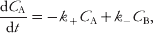
where we now introduce subscripts to denote the concentrations of molecules in the two states. A similar equation can be written for the concentration, C B, of molecules in state B. Alternatively, C A and C B are related by the fact that the total concentration is conserved:

Using Eq. (2.7) in Eq. (2.6) and solving for C A, we find
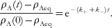
To simplify notation, we have normalized the concentration by C t; ρA(t)=C A/C t is the proportion of molecules in state A. Its value at long times, when equilibrium has reached, is
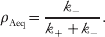
Similar results can be written for C B. The ratio of the equilibrium concentrations of the two states is known as the equilibrium constant, to be denoted as K. We have
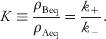
This identity can be viewed as a constraint on the rate constants. A minimum requirement on a rate theory is that the ratio of the predicted forward and reverse rate constants be the same as the equilibrium constant.
While in a bulk experiment the proportions of molecules in different states [such as the results given by Eq. (2.8)] are of interest, in a single-molecule experiment one directly observes the state of an individual molecule as a function of time. The length of stay in a state, or waiting time, is random. Equation (2.4), with k replaced by either k + or k −, gives the probability that the molecule remains in that state after time t; this is also the probability that the waiting time is longer than t. Correspondingly, the probability distributions of the waiting times, τA and τB, are

Over a long-time course, the fractions of time spent by the molecule in the two states are proportional to the average waiting times in the two states, which are 1/k + and 1/k −, respectively. The ratio of the fractions of time in the two states is thus k +/k −, which, according to Eq. (2.9), is the equilibrium constant.
In microscopic terms, a state of a molecule corresponds to a region of conformational space around a local energy minimum (or more precisely, a set of minima). One state is separated from another by energy barriers. We use x to denote a position in conformational space and U(x) as the potential energy function of the molecule. A rate description is good when jumps between the states are rare, such that, between jumps, the positions of the molecule in the conformational space are completely randomized, and consequently successive jumps are uncorrelated. In classical statistical mechanics, ‘randomized’ means that the probability that a given position x is sampled is proportional to the Boltzmann factor exp[−U(x)/k BT]. The integration of the Boltzmann factor over the conformational space of state A, ∫Adxexp[−U(x)/k BT], gives the total probability of that state. We refer to such an integral as a state-specific configurational integral. When the jumps between states A and B reach equilibrium, the probabilities, ρAeq and ρBeq, that the molecule is found in the two states are proportional to the respective configurational integrals. We then have
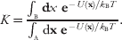
Note that the equilibrium constant, as to be expected, is completely determined by the potential energy function.
According to Eq. (2.10), the rate constant k + is the inverse of the average waiting time  . In microscopic terms,
 is the time it takes for the molecule, starting from a random position in state A to first reach a position in state B. (In subsection 3.6, this time will be referred to as the mean first passage time.) When a molecule first reaches state A, it takes some time, τAeq, for it to be equilibrated within the state. The condition for the validity of the rate description can now be expressed as
 . That this condition can be satisfied rests on the fact that, to jump from state A to state B, the molecule must cross the energy barriers separating the two states. According to the Boltzmann distribution, the barrier regions will be sampled much less frequently than the conformational space of state A. As for the magnitude of the rate constant, it can be anticipated that the activation energy, i.e., the difference in energy between the barrier regions and the conformational space of state A, is a major determinant. In addition, the type of motion that brings the molecule from state A to state B obviously should also play a role.
To recapitulate, a rate description is valid when the jumps from one state to another are rare so as to be uncorrelated. Foremost the activation energy but also the type of motion that brings about the jumps are determinants of the rate constant. Below we present two special topics. The first is a simple model designed to further contrast τAeq and  . The second concerns intermolecular transitions, as opposed to the intramolecular transitions discussed thus far.
2.1 A simple model with intra-state equilibration and inter-state jump
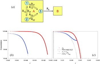
As noted above, a state consists of a set of local energy minima. Each local minimum corresponds to a microstate. Figure 2a presents a model in which state A consists of three microstates, to be referred to by index i or j, with i and j=1–3; from microstate 3 the molecule can make a jump to state B. We choose model parameters to illustrate two situations:  and
 . The results of these two situations are displayed in Fig. 2b and c, respectively.
A simple model with intra-state equilibration and inter-state jump. (a) Illustration of the model. The two states, A and B, are represented by boxes; microstates within state A are represented by circles. (b) Time dependences of σ1 and ρ1/ρAeq, representing intra-state equilibration, and of ρA, representing inter-state jump, for the following parameter values: k 12=k 21=k 13=k 23=1, k 31=k 32=2, and k tr=0·1. (c) The corresponding results when k 31 and k 32 are decreased to 0·125 and k tr is increased to 1. The results are obtained from kinetic simulations of a single molecule. Briefly, the waiting time of the molecule in an initial microstate is generated from an exponential distribution function [see Eq. (2.10)], with the average waiting time equal to the inverse of the sum of the rate constants for all the pathways leaving that microstate. The probability for taking each of these pathways is proportional to the corresponding rate constant. The results shown are the average of 106 repeat simulations; each simulation starts with the molecule in microstate 1. This simulation procedure is similar in spirit to the stochastic simulation algorithm of Gillespie (Reference Gillespie1977).

First, let us study the equilibration among the three microstates of state A, which we model as rate processes, with rate constants kij. For now jumps to state B are not considered. The rate constants for the forward and reverse transitions between two microstates, e.g., k 12 and k 21, are constrained by the corresponding equilibrium constant, which in turn is given by the ratio of the configurational integrals of the two microstates [Eq. (2.11)]. Our interest is in how the proportions of molecules in the microstates, hereafter referred to as occupation probabilities, evolve over time. We denote the occupation probabilities here as σi; the corresponding quantities when jumps to state B are allowed will be denoted as ρi (see below). Starting from any initial values σi0, σi will relax to their equilibrium values σieq, which are proportional to the respective configurational integrals. The time dependence of σi can be obtained from a kinetic simulation (see Fig. 2). In Fig. 2b, we plot σ1−σ1eq as a function of time when the initial values are σ10=1 and σ20=σ30=0 and the rate constants are k 12=k 21=k 13=k 23=1 and k 31=k 32=2. The corresponding equilibrium values are σ1eq=σ2eq=0·4 and σ3eq=0·2. The equilibration time τAeq can be estimated as the area under the (σ1−σ1eq)/(σ10−σ1eq) versus t curve; we find τAeq=0·31. Figure 2c displays the result for σ1−σ1eq when k 31 and k 32 are decreased by 16-fold to 0·125 (while all other parameters are unchanged). The equilibrium values become σ1eq=σ2eq=0·2 and σ3eq=0·8, and τAeq increases to 0·54.
We now include jumps to state B from microstate 3, again modeled as a rate process, with rate constant k tr. Both the equilibration among the three microstates and the jumps to state B affect ρi, the occupation probabilities. The latter leads to a decrease in the total occupation probability of state A, ρA=ρ1+ρ2+ρ3, over time. The decrease is governed by

We use the normalized occupation probabilities, ρi/ρA, to monitor the equilibration among the three microstates. The situation  displayed in Fig. 2b has k tr=0·1, along with the values of kij specified above. Firstly, it can be seen that the decay of ρA can be fitted well to an exponential function, which is expected if a rate description is valid [Eq. (2.4)]. The fitted rate constant, k +, has a value of 0·0196; correspondingly, the average waiting time
 is 51. Secondly, the time dependence of ρ1/ρA matches that of σ1. Thus, the equilibration time of 0·31 based on σ1 is also correct for the present case where jumps to state B are allowed. Compared to
 , we find that τAeq is two orders of magnitude shorter in the present situation. That the initial decays of ρi/ρA and σi match are easy to rationalize, since during this period very few jumps to state B occur. On the other hand, that ρi/ρA settle to the same equilibrium values σieq suggests a scenario that, when the equilibrium within state A is perturbed by a jump from microstate 3 to state B, it is recovered by re-equilibration among the microstates before the next jump occurs. This scenario also allows us to find an approximate value for the rate constant k +. Making use of the result ρ3/ρA≈σ3eq, which holds after a brief initial period, Eq. (2.12) becomes
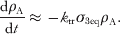
The rate constant is thus

which has a value of 0·02 for the parameters used in Fig. 2b. This predicted value is very close to the value, 0·0196, obtained above from fitting the time dependence of ρA to an exponential function.
The situation  displayed in Fig. 2c has k tr=1. Compared to the parameters used in Fig. 2b, k tr is increased by 10-fold, along with the 16-fold decrease in k 31 and k 32 stated above. For these parameters, the time dependence of ρA no longer fits well to an exponential function, and hence a rate description is not valid here. At the same time, ρ1/ρA deviates significantly from σ1, except at short times (when jumps to state B are only few). Notably, ρ1/ρA and ρA decay on a comparable timescale, validating the claim that the case under consideration has
 .
Together, the contrasting situations shown in Fig. 2b, c illustrate the point that a rate description will hold when the transitions between two states are rare enough to allow for intra-state equilibration.
2.2 Intermolecular transitions
Up to now, we have discussed transitions between states of the same molecule. Many reactions of biological interest involve the binding of two different molecules, e.g., a protein and a ligand, to form a complex. In this case, the protein molecule makes a transition from a state in which it is freely translating and rotating by itself throughout the container to a state in which its translation and rotation are coupled to those of the ligand molecule. (The alternative perspective, centered on the ligand instead of the protein, is equally valid.) Even though the transition is intermolecular instead of intramolecular, the derivation leading to Eq. (2.2) can still be considered valid, except that the ‘rate constant’ k introduced there is now proportional to the ligand concentration C L, since the probability that a protein molecule makes the transition from the free state to the protein–ligand complex in an infinitesimal time interval is proportional to C L. We thus replace k by k aC L, where k a is the new rate constant for the association of the protein molecule with the ligand molecule. The reverse process, i.e., the dissociation of the protein–ligand complex into separate protein and ligand molecules, is an example of the intramolecular transitions discussed above, since the reactant, i.e., the protein–ligand complex, is effectively one molecule. We denote the dissociation rate constant as k d. The association and dissociation can be represented by the reaction scheme

The rate equation for the protein concentration, C P, is
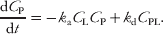
Here the forward reaction rate is second order in reactant concentration and hence that reaction is referred to as second order. When C L is a constant, which, e.g., is practically realized when the ligand is in large excess over the protein, the product k aC L can be treated as an effective rate constant. For such a pseudo-first-order situation, the solution of the rate equation can be obtained by identifying k ± in Eq. (2.8a) with k aC L and k d, respectively, leading to

where we have introduced the equilibrium constant for dissociation, or dissociation constant

Its inverse is called the association constant, denoted as K a. The equilibrium protein concentration is given by
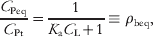
where C Pt is the total protein concentration, either in the free state or in the bound state:

and ρbeq gives the bound fraction (the unbound fraction ρueq is 1−ρbeq).
When C L cannot be treated as a constant, it is still constrained by the fact that the total ligand concentration, either free or in the complex, is fixed:

Using Eqs. (2.19) in Eq. (2.15), we find the solution for C P to be given by

where


It can be verified that when C Pt≪C Lt, Eq. (2.20) reduces to Eq. (2.16).
At long times, the equilibrium value that the protein concentration settles into is C P−. Unlike the unimolecular case [Eq. (2.8)], where the equilibrium concentration as a proportion of the total concentration is an intrinsic property of the molecule, in the bimolecular case the equilibrium protein concentration as a proportion of the total protein concentration is not an intrinsic constant; it depends on the total protein concentration and the total ligand concentration. Similar to Eq. (2.11) for the unimolecular case, we may express the association constant in terms of the configurational integrals of the protein, the ligand, and their complex. Let the potential energy functions of the three systems be U P(xP), U L(xL), and U PL(xPL). Then we have (Zhou & Gilson, Reference Zhou and Gilson2009)

In some reactions, product formation involves more than two reactant molecules. For example, many enzymatic reactions require the binding of two or more substrates to one enzyme. Compared to the binding of two molecules to form a binary complex, the chance of three molecules binding simultaneously to form a ternary complex is negligibly small. Surely the ternary complex must form in two steps: in the first step, two of the molecules bind to form an intermediate binary complex; in the second step, the third molecule binds to the pre-formed binary complex to yield the ternary complex. It can thus be concluded that all elementary reactions are either unimolecular or bimolecular.
3. Unimolecular reactions
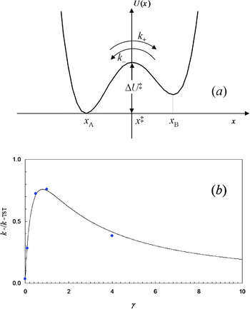
Intramolecular processes, such as protein folding or dissociation of a protein–ligand complex, are often modeled as unimolecular reactions. A simple microscopic picture of unimolecular reactions, shown in Fig. 3a, consists of a one-dimensional energy function with two wells separated by an energy barrier. The independent variable of this function is referred to as the reaction coordinate. As alluded to in section 2, both the energy function and the type of motion of the reaction coordinate are determinants of the rate constant for the transition from one well to another. Below we review some of the milestones in the development of rate theories for unimolecular reactions. We use the one-dimensional model to present the basic ideas of the rate theories and to introduce different types of motion. Several results for multi-dimensional energy surfaces and for conformations represented as discrete microstates are also noted. The interested reader may consult a related review (Hanggi et al. Reference Hanggi, Talkner and Borkovec1990) for further reading in developments before 1990.
A one-dimensional model for unimolecular reaction. (a) The potential energy function. (b) Results for the rate constant obtained from computer simulations (filled circles) and predicted by Melnikov and Meshkov [Eqs. (3.69) and (3.71); curve], for the potential energy function U(x)=(x 2−1)2, with k BT=1/4 and m=1. The simulation results are from Zhou (Reference Zhou1989), by fitting the number correlation function [Eq. (3.20)] to an exponential function.

It should be noted that what we refer to as energy functions are actually potentials of mean force. Biological processes occur in aqueous environments, but in applications of rate theories solvent degrees of freedom are almost never explicitly modeled. Rather, they are accounted for through their effects on the energy functions and on the dynamics of the reactant molecules. In addition, often only a reaction coordinate and perhaps a small number of additional coordinates closely coupled to it are explicitly modeled, and the remaining degrees of freedom of even the reactant molecules are implicitly treated as a part of the solvent environment.
Of historical importance to the present rate theories is the work of Van't Hoff (Reference Van Oijen, Blainey, Crampton, Richardson, Ellenberger and Xie1884) and Arrhenius (Reference Arrhenius1889) regarding the temperature dependence of rate constants. Van't Hoff's starting point was the now well-known equation, bearing his name, for the equilibrium constant:

where ΔH is the change in enthalpy when one reactant molecule is converted to one product molecule, which in turn is essentially identical to the change in internal energy if the reaction occurs in a dilution solution under constant pressure (Zhou & Gilson, Reference Zhou and Gilson2009). Replacing the equilibrium constant by the ratio of the rate constants [Eq. (2.9)] leads to
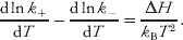
Van't Hoff reasoned that both the terms on the left-hand side of the above equation must have the form
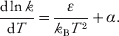
Arrhenius had an important additional insight. He reasoned that the reactant molecules that successfully convert into product molecules must be in some ‘active’ form; these active molecules are in equilibrium with all the other normal reactant molecules. The rate constant is proportional to the normal-to-active equilibrium constant, and applying Van't Hoff's equation [Eq. (3.1)] to that equilibrium constant leads to

Here ΔE‡ denotes the change in energy between an active molecule and a normal reactant molecule, i.e., the activation energy. (Mathematically Arrhenius' result is a specialization of Van't Hoff's result, with α=0 and ε=ΔE‡.) Integrating over temperature, we arrive at the more familiar form of the rate constant:
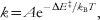
where the pre-exponential factor A is a constant of the integration. The expressions for rate constants presented below conform to Eq. (3.5), with the pre-exponential factor affected by the type of motion of the reaction coordinate.
3.1 Eyring's transition-state theory
The most influential rate theory is the transition-state theory of Eyring (Reference Eyring1935), also worked out by Evans & Polanyi (Reference Evans and Polanyi1935). It is based on three assumptions:
(i) The motion of molecules obeys Newton's equation. The potential energy function for our illustrative model is shown in Fig. 3a.
(ii) As soon as a molecule crosses the energy barrier at x=x‡, or transition state, it is considered to form the product.
(iii) Molecules in the barrier region are in thermal equilibrium with those in the energy well of the reactant state.
In the barrier region, the potential energy function is flat; hence, there the force is zero and molecules undergo free translation. If δN molecules, all with velocity v>0, are found in the region with length δl just to the left of x=x‡, then within the time interval dt each molecule moves a distance of vdt to the right and the number of molecules that cross the barrier is δN⋅(vdt/δl). Consequently, the rate constant is

where N is the number of molecules found in the reactant energy well.
Under thermal equilibrium, δN/N is the same as the ratio of the partition functions in the barrier region and in the reactant energy well:

The partition function in the barrier region is that appropriate for free translation in one dimension:

where p=mv is the momentum of a molecule along the x-direction, m is the mass, and ΔU‡ is the activation energy (Fig. 3a). Following convention we have inserted Planck's constant h to make the partition function unitless. As indicated by Eq. (3.8), the molecules in the barrier region have a continuous distribution of velocities; therefore, the velocity v appearing in Eq. (3.6) should be replaced by its average:

where θ(v), a Heaviside function with value 1 if v>0 and 0 otherwise, is used to select only positive velocities. Combining the above results, we find
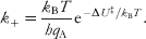
We now discuss the calculation of q A. If the problem is treated according to classical statistical mechanics, we have

Equation (3.10) becomes
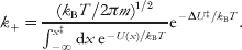
Note that Planck's constant drops out of the final result for k +, as to be expected from a classical treatment. For later use, we rewrite it in the form
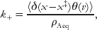
where 〈···〉 denotes an average with the canonical-ensemble equilibrium probability density

δ(x) is a delta function, and

is the equilibrium occupation probability in state A. The corresponding result for k − is obtained by replacing ρAeq with ρBeq in Eq. (3.12b). It can then be easily seen that the ratio k +/k − is the same as the equilibrium constant ρBeq/ρAeq, as demanded by Eq. (2.9). We may further make a harmonic approximation of the potential energy function around the minimum x A of the reactant well:

Using this approximation and evaluating the configurational integral in Eq. (3.12a), the rate constant is now given by
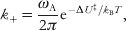
where ωA=f A1/2 is the angular frequency of the harmonic oscillation around x=x A.
With the harmonic approximation of the potential energy function, a quantum treatment for calculating q A is possible. Essentially q A is the partition function of a harmonic oscillator, given by

where ħ=h/2π. Equation (3.10) is now

This result was first derived by Herzfeld (Reference Herzfeld1919) for the dissociation of a diatomic molecule. In the high-temperature limit, q A→k BT/ħωA, and we recover the classical result of Eq. (3.16). This is to be expected, since quantum statistical mechanics approaches the classical limit at high temperatures.
Below we further comment on the approximation of the transition-state theory and a common misunderstanding of the theory.
3.1.1 Approximation of the transition-state theory
The nature of the approximation of the transition-state theory can be elucidated in the context of a more exact microscopic formulation of the rate constant. Equation (2.8a), the solution of the rate equation, states that the relaxation of ρA, the occupation probability in the reactant state, toward its equilibrium value is an exponential, with the relaxation time τrxn=(k ++k −)−1. Microscopically ρA is the average of a variable that has value 1 if the molecule occupies the reactant well and 0 otherwise:

Now Onsager's regression hypothesis states that the regression of microscopic thermal fluctuations at equilibrium follows the macroscopic law of relaxation of small non-equilibrium disturbances (Onsager, Reference Onsager1931). Accordingly,
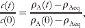
where

is the correlation function of the instantaneous fluctuation θ(x‡−x(t))−ρAeq, and is referred to as the number correlation function. Noting that θ2(x)=θ(x) and 1−ρAeq=ρBeq, it can be easily shown that c(0)=ρAeqρBeq. Now Eq. (2.8a) becomes
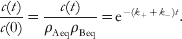
To make connection with the transition-state theory, we take the time derivative of Eq. (3.22):
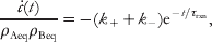
where a dot represents a derivative. The time derivative of the number correlation function is given by

which can be interpreted as the reactive flux, i.e., the flux across the dividing surface given that the reactant molecule starts there and is found in the product well time t later (Chandler, Reference Chandler1978). As discussed in section 2, a rate description is valid only when there is a significant separation in timescales between intra-state equilibration (τeq) and inter-state transitions (τrxn). In that case, the number correlation function is exponential at times longer than τeq. Because of the separation in timescales, there exist intermediate times, denoted as Δt, such that τeq≪Δt≪τrxn. At these intermediate times, exp(−Δt/τrxn) is very close to 1; therefore Eq. (3.23) becomes (Chandler, Reference Chandler1978; Yamamoto, Reference Yamamoto1960)

Correspondingly,

The transition-state theory amounts to setting Δt in the last equation to 0+, which denotes a time that is greater than 0 by an infinitesimal amount:

The equivalence of Eqs. (3.26) and (3.12b) is seen when one realizes that x(0+)>x‡ if and only if v(0)>0. A related approach for formulating the rate constant is presented in subsection 3.2.
To recapitulate, the transition-state theory predicts the rate constant from the initial reactive flux, when the exponential relaxation of the number correlation function has not been established. The correct formulation is to use the reactive flux at the intermediate times Δt. Since the number correlation function decays with time, it can be expected that the transition-state theory always overestimates the rate constant. Although Eyring recognized the overestimation and introduced a transmission coefficient, it was not possible to calculate the transmission coefficient within the transition-state theory itself. That the transition-state theory provides an upper bound for the rate constant is the basis of variational transition-state theory, which seeks a dividing surface that minimizes the rate constant calculated by the transition-state theory (Keck, Reference Keck1960; Wigner, Reference Wigner1937).
We end this subsubsection with some results that are related to the preceding formulation and will become useful below. When the motion of the reaction coordinate is governed by the Langevin equation, Onsager's regression hypothesis [Eq. (3.20)] has been proven explicitly (Zhou, Reference Zhou1989). It is assumed the initial probability density is an equilibrium distribution confined to the reactant state. Then


where ρN(x,v,t|x 0,v 0) is the conditional probability density for finding the molecule at x with velocity v at time t given that it was at x 0 with velocity v 0 at t=0; ρN(x,t|x 0) is the reduced conditional probability density in x for an equilibrium distribution in v 0. The subscript ‘N’ has a special meaning: it signifies that the probability density satisfies natural boundary conditions, i.e., the decay to zero at x=±∞ because of the infinite potential energies there. These boundary conditions are to be distinguished from, e.g., absorbing boundary conditions that are introduced below for various purposes. By design ρA(0)=1. Instead of finding k ++k − from the time derivative of the number correlation function, its inverse, i.e., the relaxation time, is given by the time integral [see Eq. (3.22)] (Skinner & Wolynes, Reference Skinner and Wolynes1978):

Now expressing c(t) in terms of ρA(t) [Eq. (3.20)], we find

Correspondingly (Zhou, Reference Zhou2005a),

3.1.2 Multi-dimensional transition-state theory and a common misunderstanding
Although we have so far presented the transition-state theory for a one-dimensional potential energy surface, the theory was originally derived for molecules described by a multi-dimensional energy function, to be denoted as U(x). It is assumed that a suitable reaction coordinate, x, is found; a surface, x=x‡, is appropriate as a dividing surface between the reactant and the product states, and x, at least around the minimum of U(x) on the dividing surface, is uncoupled to the remaining degrees of freedom. Now the whole dividing surface x=x‡ is the transition state. Let the partition function in the reactant well, with its minimum chosen as the reference of potential energy, still be denoted as q A and the partition function for all coordinates other than x, with x fixed at x‡ and the minimum of U(x) on the dividing surface chosen as the reference of potential energy, be denoted as q′‡. Then Eq. (3.10) for the rate constant is generalized to
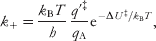
where the activation energy ΔU‡ is the difference between the minima of U(x) on the dividing surface and in the reactant well. The prime in the partition function q′‡ is very important; again, it signifies that the reaction coordinate is left out of the calculation of this partition. In the one-dimensional model discussed above, there are no coordinates other than the reaction coordinate, and q′‡ would be 1.
Often q′‡ is mistakenly thought as the partition function of the transition state. Following this mistaken notion, one would be misled to think that  defines the free-energy difference, to be denoted as ΔG‡, between the transition state and the reactant state:
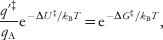
which in turn transforms Eq. (3.31) into
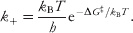
While mathematically the last expression cannot be faulted, it nevertheless results in the misleading interpretation that ΔG‡ is the activation energy and k BT/h is the pre-exponential factor. The presence of Planck's constant in such a pre-exponential factor would suggest that quantum effects persist at all temperatures. In reality, q A involves one additional coordinate than q′‡; at high temperatures this additional coordinate would contribute a factor that cancels the h in k BT/h, as illustrated above on the one-dimensional model.
We again stress that in calculating q′‡ the reaction coordinate is left out, and q′‡ is not the partition function of the transition state. In fact, for the one-dimensional model, we have defined a partition function of the transition state [Eq. (3.8)], with the reaction coordinate not fixed at a single value (as would be required in calculating q′‡) but extending over a range δl. A rigorous implementation of the multi-dimensional transition-state theory will be illustrated below in subsection 3.3.
3.2 Kramers' turnover problem
In a sense, assumptions (i) and (iii) that lead to the transition-state theory are contradictory to each other. If the motion of molecules, each with a single degree of freedom along the reaction coordinate, is governed by Newton's equation, then the energy of each molecule would be conserved. Low-energy molecules would stay in the reactant well, and higher-energy molecules would stay in the barrier region; these two types of molecules would not be able to mix and equilibrate. In reality, the reaction coordinate is coupled to other degrees of freedom of a reactant molecule and to solvent molecules, which effectively serve as a thermal bath that allows for energy dissipation and thermal equilibration. In Kramers' theory (Kramers, Reference Kramers1940), the motion along the reaction coordinate is governed by the Langevin equation:
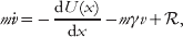
which augments Newton's equation by two additional forces: a frictional force, −mγv, which serves to dissipate the energy of the molecule,; and a random force,  , which serves to agitate the molecule, leading to thermal equilibration. The random force has a Gaussian distribution, with zero mean and correlation given by

which is a form of the fluctuation–dissipation theorem.
Because of the random force, the trajectory of the molecule is not deterministic but stochastic. Complementary to stochastic trajectory, we may describe the microscopic behavior of the molecule by the probability density, ρ(x,v,t), in position and velocity as a function of time. This probability density satisfies the Fokker–Planck equation

It can be checked that the canonical-ensemble equilibrium distribution given by Eq. (3.13) is a stationary solution of the Fokker–Planck equation.
Let us first discuss the limits of high and low frictions. When γ→∞, the change in x is slow and the relaxation in v is fast. Then the inertial term on the left-hand side of the Langevin equation can be neglected, leading to
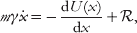
which is the governing equation for Brownian (or diffusive) motion of x.
Correspondingly, the probability density in x, ρ(x,t), satisfies the Smoluchowski equation

where D=k BT/mγ is the positional diffusion constant. The equilibrium distribution is
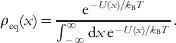
In the high-friction limit, positional diffusion from the reactant well to the product well becomes rate limiting. It can thus be expected that in this limit k +∝D∝1/γ.
In the low-friction limit, the total energy, E=mv 2/2+U(x), is nearly conserved, and the motion of the molecule can be described as diffusion among different energy levels. The probability density in E, ρ(E,t), satisfies the equation (Zwanzig, Reference Zwanzig2001)

where

is the action for the periodic orbit with total energy E and

is the angular frequency of the orbit. Note that I(E) is also the area inside the orbit in phase (i.e., x and p) space, and dI(E)/dE=2π/ω(E) is the density of states. Here the equilibrium distribution ρeq(E)∝[2π/ω(E)]exp(−E/k BT). Comparing Eqs. (3.38) and (3.36), it can be seen that the energy diffusion constant, DE, is proportional to γ. Therefore, in the low-friction limit one expects k +∝DE∝γ.
Putting the results in the two limits together, one sees that the rate constant increases with increasing γ when γ is small and decreases with increasing γ when γ is large (Fig. 3b). It can thus be expected that the value of k + reaches a maximum at an intermediate γ and decreases to zero when γ approaches either zero or infinity. This dependence of the rate constant on friction is known as Kramers' turnover.
Kramers derived expressions for the rate constant for different ranges of the friction coefficient. His approach can be explained from the perspective of a hypothetical bulk experiment (Farkas, Reference Farkas1927; Zhou, Reference Zhou2005a). In this experiment, molecules are prepared at the reactant state with a concentration C. Whenever a transition is made to the product state, the molecule is immediately removed, as if there is an absorbing trap, and the reactant pool is replenished so that the reactant concentration is always maintained at C. After a brief transient period (lasting ~τeq), a steady state will set in. The steady-state flux will be [see Eq. (2.2)]

Rearranging, we find

The rate constant is thus given by the ratio of the steady-state flux and the reactant population. Note that the reactive-flux formulation, Eq. (3.25b), of the rate constant can be viewed as a special case of the flux-over-population formulation. As observed already, the transition-state theory [Eq. (3.26)] makes the approximation of replacing the ‘steady-state’ reactive flux by its initial value.
To implement the flux-over-population formulation, one would find a steady-state probability density that maintains the equilibrium distribution in the reactant well and satisfies the absorbing boundary condition in the product well. The implementation is straightforward in the high-friction regime, where the motion of the molecule is modeled as positional diffusion. A steady-state probability density corresponds to a constant flux:

The appropriate boundary conditions are


Solving Eq. (3.41) for ρss(x) subject to the condition of Eq. (3.42a), we find

Using Eq. (3.42b), we find the flux
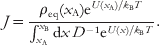
Now with the condition in Eq. (3.42a), the population in the reactant well is

The rate constant is finally

Making the harmonic approximation of Eq. (3.15) for the potential around x A and a similar approximation

for the potential around the top of the barrier, we find
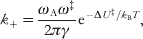
where ω‡=(f‡)1/2. Equation (3.44) is still valid when D is a position-dependent diffusion coefficient, i.e., D(x). The first integral in the denominator is then dominated by the region around the maximum of an effective potential, U(x)−k BTlnD(x). The location of the maximum, which was referred to as the kinetic transition state (Chahine et al. Reference Chahine, Oliveira, Leite and Wang2007), and the effective activation energy can be quite different from those of the original potential.
As shown below in subsubsection 3.6.2, the ratio ρss(x)/ρeq(x) is the splitting probability, denoted as ζA(x), which is the probability that a molecule, started at x, will first reach the reactant well bottom instead of the product well bottom. When x is in the reactant well, ζA(x) is very close to 1. Around x=x‡, ζA(x) undergoes a rapid transition, to ~1/2 at x=x‡, and to 0 a small distance thereafter.
By a similar procedure, we find the rate constant in the low-friction limit:


where

with x tA being the left-hand-side turning point, i.e., the solution of U(x)=ΔU‡ to the left of x=x A. A comment on the upper limit of the second integral in Eq. (3.47a) is in order. Orbits with energies higher than ΔU‡ will traverse both the reactant and the product wells. Setting the upper limit of the integration to ΔU‡ amounts to assuming that all molecules moving along those orbits would be trapped in the product well. However, it should be recalled that, in the flux-over-population formulation, the absorbing boundary is set around x=x B, i.e., inside the product well. For molecules with E>ΔU‡, this absorbing boundary traps only those moving to the left (i.e., v<0) but not those moving to the right (i.e., v>0). This ‘split’ boundary condition is treated properly later by Melnikov & Meshkov (Reference Melnikov and Meshkov1986); see subsection 3.4.
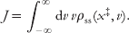
For moderate to high frictions, we again seek a steady-state probability density ρss(x,v), which takes the equilibrium distribution around the bottom of the reactant well and becomes zero at the bottom of the product well.Footnote 1 The flux from the reactant well to the product well is
We write ρss(x,v) as

The splitting probability ζA(x,v)=ζ(x,–v) (the appearance of the negative sign will be explained in subsubsection 3.6.2). ζ(x,v) satisfies the equation

with the boundary conditions

We now solve for ζ(x,v) around x=x‡. Applying the harmonic approximation of Eq. (3.45), Eq. (3.51a) becomes

The trick is to seek a set of parallel lines in phase space, over each of which ζ(x,v) is a constant; the value of this constant changes as the line moves from the reactant well to the product well. Let each line be represented by the equation λ(x−x‡)−v=u, where u dictates the location of the line. The desired condition is satisfied by choosing

Correspondingly, the solution of Eq. (3.51b) is

which has a transition in value around u=0, i.e., the line that goes through the point (x, v)=(x‡, 0). If this transition is essentially complete within the range where the harmonic approximation of the potential around x=x‡ holds, then the boundary conditions are satisfied by setting

The rate constant can finally be calculated as
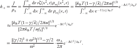
It can be easily checked that Eq. (3.54) reduces to the high-friction limit given by Eq. (3.46) when γ→∞. However, when γ→0, Eq. (3.54) does not reduce to the low-friction limit given by Eq. (3.47b). Instead, in this limit it reduces to the transition-state theory result given by Eq. (3.16). The validity of Eq. (3.54) requires that the transition of ζA(x,v) occurs in a range where the harmonic approximation of the potential around x=x‡ holds. As noted by Melnikov & Meshkov (Reference Melnikov and Meshkov1986), this range is proportional to γ−1/2, which extends to infinity as γ→0. That explains why Eq. (3.54) is only valid for moderate to high frictions (see also footnote 1).
In summary, Kramers has shown that the rate constant is proportional to γ when γ is low and proportional to γ−1 when γ is high. The rate constant exhibits a maximum at an intermediate friction. However, Kramers did not find an expression for the rate constant that works for the full range of friction.
3.3 Friction with memory: Grote–Hynes theory
The Langevin equation (3.32) is a special case of a more general class of equation of motion

known as the generalized Langevin equation. The friction coefficient here has the form of a memory kernel. Correspondingly, the correlation function of the Gaussian random force is

Grote & Hynes (Reference Grote and Hynes1980) used the generalized Langevin equation to model the motion along the reaction coordinate and derived the counterpart to Kramers' result [Eq. (3.54)] for the rate constant at moderate to high frictions.
The Grote–Hynes theory is based on a formulation of the rate constant derived from the so-called stable states picture (Northrup & Hynes, Reference Northrup and Hynes1980). As explained in the preceding subsection, the steady-state probability density appropriate for calculating the rate constant is nearly identical to the equilibrium distribution in the reactant well but deviates significantly from it in the barrier region. Northrup & Hynes (Reference Northrup and Hynes1980) thus introduced an intermediate state, I, in addition to the ‘stable’ states A and B. The dividing line between A and I is located at a position where the steady-state probability density starts to deviate from the equilibrium distribution; a similar dividing line can be defined between B and I. These two positions will be denoted as x A−I and x I−B, respectively. The rate constant is given by

where the first flux is across the A–I dividing line at time 0 and the second flux is across the I–B dividing line at time t. The initial probability density is an equilibrium distribution in A; an absorbing boundary is set in B. Equation (3.57a) is closely related to the reactive-flux formulation [Eq. (3.25b)] of the rate constant.
Similar to Kramers, Grote and Hynes assumed that the harmonic approximation of Eq. (3.45) applies to the entire region of I. They then extended this downward parabola indefinitely beyond x=x A-I and x=x I-B. Let the conditional probability density in this extended parabola be ρN(x,v,t|x 0,v 0). Note that ρN(x,v,t|x 0,v 0) naturally satisfies the desired absorbing boundary condition. The rate constant can now be expressed as

The conditional probability density in a parabolic potential is Gaussian. Evaluating all the integrals involved, the final result is

where the Grote–Hynes ‘reactive’ frequency ωGH is the positive root of the equation

with  denoting the Laplace transform of the memory kernel. For the memory-free friction, ξ(t)=2γδ(t), Eq. (3.58) gives
 , and one recovers Kramers' result, Eq. (3.54).
As alluded to in the preceding subsection, friction arises from coupling of the reaction coordinate to other degrees of freedom of the reactant molecule and to solvent molecules, serving as a thermal bath. A simple model for a thermal bath consists of a set of n harmonic oscillators, with the potential energy (Zwanzig, Reference Zwanzig2001)
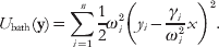
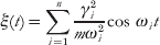
The whole system, reaction coordinate plus thermal bath, satisfies Newton's equation. By eliminating the bath coordinates, yj, one arrives at the generalized Langevin equation (3.55). The memory kernel is given by
and the ‘random’ force is given by

where x 0 is the initial value of x, yi 0 are the initial values of the bath coordinates, and vi 0 are the corresponding initial velocities. Equation (3.60) shows that memory kernels, such as that of an exponential form, typically used to model unimolecular reactions correspond to an infinite set of bath oscillators that spans a continuous spectrum of frequencies. For later reference, we note that the Laplace transform of the memory kernel in Eq. (3.60) is given by
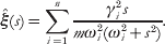
With a small set (n~30) of oscillators, computer simulations (Zhou & Zwanzig, Reference Zhou and Zwanzig2002) show that the Grote–Hynes theory provides a reasonable estimate for the rate constant at moderate frictions. However, at high frictions, the number correlation function becomes non-exponential, and the decay is much slower than that expected from the Grote–Hynes theory.
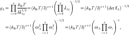
Interestingly, Pollak (Reference Pollak1986) found that, when the multi-dimensional transition-state theory [Eq. (3.31)] is applied to the whole system of reaction coordinate plus thermal bath, the Grote–Hynes result, Eq. (3.57c), is derived. We outline this derivation here, mainly to illustrate the use of the multi-dimensional transition-state theory. The implementation of Eq. (3.31) entails evaluating two partition functions, q A and q′‡. To evaluate q A, we again use the harmonic approximation of Eq. (3.15). Then the system is equivalent to a set of n+1 harmonic oscillators. The eigenvalues, λAi, i=0 to n, of the [mass-scaled; cf. Eq. (3.81)] force-constant matrix, fA, give the angular frequencies as λAi1/2. In the classical limit, each oscillator contributes a factor k BT/ħAi1/2 to the partition function. Therefore,
where det denotes determinant. To calculate q′‡, we apply the harmonic approximation of Eq. (3.45) and carry out a similar normal mode analysis around the saddle point of the multi-dimensional energy function U(x)+U bath(y). The force-constant matrix f‡ in the barrier region has one negative eigenvalue, −λ0‡, and n positive eigenvalues, λi‡, i=1 to n. The value of λ0‡ is determined by

where I denotes the identity matrix. The last equation is satisfied when

Comparison with Eq. (3.58) shows that  =ωGH. We define the mode corresponding to the negative eigenvalue as the modified reaction coordinate. This mode, with coordinate denoted as x′, does not coincide with the original reaction coordinate x and instead is a linear combination of x and the bath coordinates. For later use we denote the value of x′ at the saddle point as x′‡. With x′ as the new reaction coordinate, we have
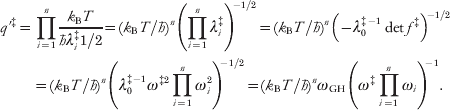
Inserting Eqs. (3.63) and (3.66) into Eq. (3.31), we indeed arrive at the Grote–Hynes result, Eq. (3.57c). Note that this rate constant can be written in the form

The above derivation amounts to choosing x′=x′‡ as the dividing surface of the multi-dimensional system of reaction coordinate plus thermal bath. Had we chosen x=x‡, based on the original reaction coordinate, as the dividing surface, we would have derived the standard transition-state theory result, Eq. (3.16). Pollak's use of a dividing surface based on the modified reaction coordinate can thus be seen as a form of variational transition-state theory. Berezhkovskii et al. (Reference Berezhkovskii, Pollak and Zitserman1992) have, in fact, carried out variational transition-state theory calculations using a planar dividing surface. They found that, when the harmonic approximation of Eq. (3.45) is invoked for the potential function, the optimized planar dividing surface is x′=x′‡. However, when anharmonicity is accounted for, the optimized planar dividing surface differs from x′=x′‡ in direction and no longer goes through the saddle point if U(x) is asymmetric with respect to x=x‡.
3.4 Solution to the turnover problem
As noted in subsection 3.2, a proper calculation of the rate constant at low frictions should account for a split boundary condition arising from the absorbing boundary around the bottom of the product well, which traps molecules moving to the left but not those moving to the right. Melnikov & Meshkov (Reference Melnikov and Meshkov1986) dealt with this split boundary condition by the Wiener–Hopf method. When the rate constant is written in the form

where k +TST is given by Eq. (3.16), their result for the transmission coefficient is
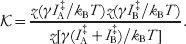
In the last expression I A‡ is given by Eq. (3.48), I B‡ is the counterpart for the product well, and the function z(x) is given by

which goes to x when x→0 and to 1 when x→∞.
In the low-friction limit, Eq. (3.69) gives  =γI A‡I B‡/(I A‡+I B‡)k BT. This differs from the corresponding result of Kramers, γI A‡/k BT [see Eq. (3.47b)] by a factor I B‡/(I A‡+I B‡), which arises from accounting for the fact that the orbit with total energy ΔU‡ traverses both the reactant and the product wells. In the high-friction limit, Eq. (3.69) predicts =1, i.e., the transition-state theory result. The validity of Eq. (3.69) is thus restricted to low to moderate frictions. Melnikov and Meshkov recognized that, when the transmission coefficient of Eq. (3.69) is multiplied to Eq. (3.54), which is Kramers' result for the rate constant at moderate to high frictions, the resulting expression

is numerically accurate for both the low to moderate and the moderate to high ranges of friction. This expression can thus be used for the full range of friction. Computer simulations have shown that Eq. (3.71) is indeed highly accurate for all frictions (Zhou, Reference Zhou1989) (see Fig. 3b).
Pollak et al. (Reference Pollak, Grabert and Hanggi1989) subsequently developed an improved solution to the turnover problem. Following the work of Pollak (Reference Pollak1986) outlined above, they modeled the thermal bath as a set of harmonic oscillators. The rate constant at low frictions was derived by studying the sampling of energy levels associated with the modified reaction coordinate x′, not those associated with x as done by Kramers and by Melnikov and Meshkov. When the friction is taken to the high range, this rate constant becomes identical to the result of Pollak (Reference Pollak1986), which was specifically derived for that range of friction. Therefore, the theory of Pollak et al. works for the full range of a friction with memory. Its predictions are found to agree well with results from computer simulations of Straub et al. (Reference Straub, Borkovec and Berne1986).
3.5 Multi-dimensional potential energy functions
A description restricted to a single reaction coordinate has limitations. Often it makes sense to explicitly consider other closely coupled coordinates. Below we present two perspectives on how to deal with motions on multi-dimensional energy surfaces in modeling rate processes.
3.5.1 Langer's generalization of Kramers' result and further developments
Following Kramers' work on a one-dimensional system, Langer (Reference Langer1969) studied the rate of escape from a multi-dimensional energy well through a saddle point. Consider first the case where motions along the coordinates, xi, collectively denoted as x, are diffusive. Then the probability density ρ(x, t) satisfies the multi-dimensional Smoluchowski equation
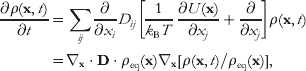
where ρeq(x)∝exp[−U(x)/k BT], and the diffusion matrix D is assumed to be position independent. [It should be noted that, for a polyatomic reactant molecule, the diffusion matrix can be very different in different parts of the conformational space (see, e.g., McCammon & Harvey, Reference Mccammon and Harvey1987). This positional dependence of D can significantly affect the reaction paths and rate constant, as already emphasized for diffusion along a one-dimensional reaction coordinate (subsection 3.2). In higher dimensions, the minimum-resistance path from the reactant well to the product well has been calculated for a position-dependent diffusion matrix by a variational approach (Berkowitz et al. Reference Berkowitz, Morgan, Mccammon and Northrup1983).] Around the bottom of the reactant well, located at x=xA, a harmonic approximation is made:

All the eigenvalues of the force-constant matrix eA are assumed to be positive. Around the saddle point x=x‡, another harmonic approximation is made:

One of the eigenvalues of the force-constant matrix e‡ is assumed to be negative and all others are positive.
Adopting Kramers' trick, Langer sought for a set of parallel planes near the saddle point, over each of which the splitting probability ζA(x)=ρss(x)/ρeq(x) is a constant. This condition is satisfied when the normal of the planes is the eigenvector, s, corresponding to the negative eigenvalue, −ω+‡, of the matrix (k BT)−1e‡⋅D. This negative eigenvalue is determined by

and the parallel planes are specified by the equation

The splitting probability around the saddle point is given by

where the magnitude of s is chosen so that

According to Eq. (3.76), the splitting probability has value 1/2 on the plane s⋅(x−x‡)=0. This plane, which goes through the saddle point, is thus the stochastic separatrix (see subsubsection 3.6.2 below). Note that, when the diffusion matrix is highly anisotropic, the eigenvector s, which is normal to the stochastic separatrix, may be very different from the eigenvector of the force-constant matrix e‡ corresponding to its negative eigenvalue.
Finally, the flux-over-population formulation gives the rate constant as
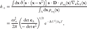
which has the same structure as Eq. (3.67). Specializing to a one-dimensional model, we recover Kramers' result [Eq. (3.46)] for high frictions. Interestingly, Berezhkovskii & Szabo (Reference Berezhkovskii and Szabo2005) showed that, if a one-dimensional reaction coordinate, x, is chosen along the eigenvector s in the multi-dimensional space, then Langer's result is identical to Kramers' one-dimensional result if the one-dimensional potential is calculated as the potential of mean force in x and the diffusion constant along x is chosen as s·D·s.
Now consider the case where motions along the coordinates are governed by the Langevin equation, which here takes the form

where mi are the masses corresponding to coordinates xi. Let the total number of coordinates be n. (For a polyatomic reactant molecule, overall translation and rotation correspond to zero eigenvalues of the force-constant matrix; such coordinates are assumed to be appropriately eliminated.) To simply notation, we absorb each mass into the corresponding coordinate and velocity; i.e., mi 1/2xi and mi 1/2vi will hereafter be written as xi and vi. The probability density ρ(x, v, t) satisfies the n-dimensional Fokker–Planck equation
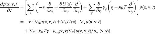
where ρeq(x, v)∝exp[–(U(x)+(1/2)v⋅v)/k BT].
Again, we seek for a set of parallel planes over which ζ(x, v)=ρss(x, v)/ρeq(x, v) is uniform. [The splitting probability ζA(x, v) is ζ(x, −v).] The normal of these planes is the eigenvector corresponding to the negative eigenvalue, −ω+‡, of the 2n×2n matrix

where 0 and I are n×n zero and identity matrices, respectively; f‡ is the n×n mass-scaled force-constant matrix, related to the original force-constant matrix e‡ via

and γ is the n×n matrix with elements γij. The eigenvalue is determined by

Note that, at high frictions, the  term is negligible, and Eq. (3.82) reduces to Eq. (3.74). Let the first and last n components of the eigenvector be denoted as s and t, respectively. The equation of the parallel planes is then

Around the saddle point, ζ(x, v) is given by

where the magnitudes of s and t are chosen so that

Finally, the flux-over-population formulation gives the rate constant as
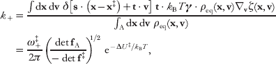
where fA is the n×n mass-scaled force-constant matrix at the bottom of the reactant well. Specializing to a one-dimensional model, we recover Kramers' result [Eq. (3.54)] for moderate to high frictions.
Berezhkovskii et al. (Reference Berezhkovskii, Pollak and Zitserman1992) considered the case where each coordinate of the multi-dimensional reactant system is coupled to a thermal bath consisting of a set of harmonic oscillators. Motion along each coordinate is then governed by a generalized Langevin equation [Eq. (3.79) with friction coefficients replaced by memory kernels]. They carried out variational transition-state theory calculations on the high-dimensional system of reactant plus thermal baths, using a planar dividing surface. Within the harmonic approximations of Eqs. (3.73), the rate constant is given by Eq. (3.86), but with the governing equation for ω+‡ generalized to

where  is a matrix with elements given by the Laplace transform of the memory kernels. A more cumbersome way to derive Eqs. (3.86) and (3.87), when motions on the multi-dimensional energy function are governed by generalized Langevin equations, is to first transform these coupled equations into an equation of motion for a single reaction coordinate, with a more complicated memory kernel, and then apply the Grote–Hynes theory (subsection 3.3) (Nitzan, Reference Nitzan1987).
As an aside, we note that the expression of the rate constant in terms of a time integral, Eq. (3.30), can be generalized to the present case of a multi-dimensional energy function. The result is (Bicout & Szabo, Reference Bicout and Szabo1997; Zhou, Reference Zhou2005a)

where θA(x) has value 1 if x is in the reactant well and 0 otherwise, and ρN(x, t |x0) is the conditional probability density satisfying natural boundary conditions. This result will find use in the next section.
3.5.2 Agmon–Hopfield model
Agmon & Hopfield (Reference Agmon and Hopfield1983) considered the situation where an intramolecular reaction, such as electron transfer or geminate binding, is coupled to conformational fluctuations of the protein molecule. To model the situation, the approach presented so far would suggest that one treats explicitly the motion along the reaction coordinate x (e.g., the distance between the germinate ligand and its binding site) and accounts implicitly for the conformational fluctuations through their effects on the potential energy and the friction coefficient for x (see, e.g., D'Abramo et al. Reference D'Abramo, Di Nola and Amadei2009; Schaad et al. Reference Schaad, Zhou, Szabo, Eaton and Henry1993). Agmon and Hopfield took the opposite approach. The intramolecular reaction is implicitly modeled by a rate constant, k +, which depends on the protein conformation, here denoted with coordinate y. The conformational fluctuations are modeled explicitly as diffusion on an effective potential surface, U(y). On account of the reaction, the probability density ρ(y, t) satisfies the diffusion-reaction equation

where D is the effective diffusion constant. For a given normalized initial distribution ρ(y, 0), the quantity of interest is the survival probability
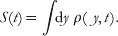
Integrating both sides of Eq. (3.89) over y, we have

In general, the rate coefficient, k(t), defined above is time dependent.
In the limit that diffusion along y is infinitely slow, the reactions at different y values proceed independently. Hence, as D→0,

and the survival probability is
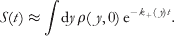
In the opposite limit D→∞, equilibration among different y values occurs quickly, and ρ(y, t) is proportional to the equilibrium distribution, ρeq(y)=exp[−U(y)/k BT]/∫dy exp[−U(y)/k BT], but with a magnitude that decreases with increasing time. Then the rate coefficient k(t) in Eq. (3.90b) is simply the equilibrium average of k +(y):

and

becomes exponential. For intermediate values of D, Eq. (3.89) can only be solved numerically.
The simple model introduced in subsection 2.1 has the flavor of the Agmon–Hopfield model. Here motion (i.e., jumps) along the y-coordinate (i.e., discrete microstates) models the equilibration within the reactant state. Like the D→∞ limit just presented, fast intra-state equilibration leads to an exponential decay of the reactant population, and the decay constant is given by the equilibrium average of rate constants among the microstates [see Eq. (2.13b)].
3.6 Two useful quantities
3.6.1 Mean first passage time
As alluded to in section 2, the rate constant k + is essentially the inverse of the mean first passage time from the reactant well to the product well. Formally, the mean first passage time, τFP, is the average time for a molecule to reach a boundary for the first time. That boundary is absorbing since the molecule never returns from it. τFP can be calculated from the survival probability, S(t), i.e., the probability that the molecule has not reached the absorbing boundary after a waiting time t. It is easy to see that the probability density, φ(t), of the first passage time t is  . Hence,

Let the molecule be specified by coordinates collectively denoted as w (which could be just spatial coordinates x or both x and the corresponding velocities v). Suppose that the probability density ρ(w, t) is governed by
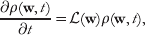
where  (w) is an operator like those in Eqs. (3.72) and (3.80). The equilibrium distribution, ρeq(w), is a stationary solution. The survival probability S(t | w0) starting from the initial position w0 satisfies (Pontryagin et al. Reference Pontryagin, Andronov and Vitt1933)
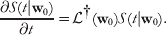
The adjoint operator is given by (Risken, Reference Risken1989)

where Ɛw0 means that the sign of each velocity component in w0 is negated. Integrating both sides of Eq. (3.95) over time leads to

For the problem of diffusive motion on the one-dimensional energy surface of Fig. 3a, with an absorbing boundary at x=x B, the solution of Eq. (3.97) is (Szabo et al. Reference Szabo, Schulten and Schulten1980)

Compared with Eq. (3.44), τFP(x A) is almost identical to the inverse of Kramers' result for the rate constant, except that the upper limit of the second integral here is x, not x‡. Numerically, this difference hardly matters since the first integral is dominated by a region around x=x‡.
An elegant application of mean first passage time is in modeling diffusive motion on a rough potential surface (Zwanzig, Reference Zwanzig1988). Consider a potential function given by

where U 0(x) is smooth and U 1(x) is a rapidly oscillating perturbation. Over the range, Δx, in which U 1(x) oscillates, U 0(x) can be considered as a constant; hence,

Over a range much longer than Δx, the above integral can then be evaluated as the integral of  . Hence,

Similarly,

with ψ+(x) defined analogous to ψ−(x). The mean first passage time of Eq. (3.98) now becomes

which is the same as if the molecule moves on an effective potential energy U 0(x)+ψ–(x) with an effective diffusion constant

Because  , roughness in the potential always leads to a reduction in diffusion constant. This provides a simple explanation for the decrease in diffusion constant when a protein moves from three-dimensional diffusion in the bulk solution to one-dimensional diffusion along a DNA, as speculated previously (Berg et al. Reference Berg, Winter and Von Hippel1981; Schranner & Richter, Reference Schranner and Richter1978) [see subsubsection 4.3.7; an alternative, or additional proposed mechanism is that, while sliding along a groove of the DNA, the protein also rotates around the DNA axis, and this coupled rotation encounters significant solvent friction (Schurr, Reference Schurr1979)].
When U 1 is random, and follows a Gaussian distribution with zero mean and variance ε, one finds ψ+(x)=ψ−(x)=ε2/2k BT. Then the effective potential is changed by a trivial constant ε2/2k BT, but the effective diffusion constant is reduced to Dexp[−(ε/k BT)2], with the exponent having a quadratic dependence on temperature. Such a T 2 dependence of the effective diffusion constant has been found for a random energy model of protein folding (Bryngelson & Wolynes, Reference Bryngelson and Wolynes1989).
3.6.2 Splitting probability
In subsection 3.2 and subsubsection 3.5.1, we introduced the splitting probability via its relation to a steady-state probability density. This relation can be generally written as
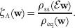
The steady-state probability density satisfies

with the boundary conditions


where xA and xB represent the bottoms of the reactant and product wells, respectively. It appears that the relation between ζA(w) and ρss(w) has not been recognized previously. We now outline its proof.
The splitting probability ζA(w) satisfies the equation (Gardiner, Reference Gardiner1985)
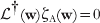
with the boundary conditions


[If the roles of states A and B were reversed, Eqs. (3.103) and (3.104) would define the splitting probability, ζB(w), for the molecule to first reach the product state instead of the reactant state. It is clear that ζB(w)=1−ζA(w).] Combining Eqs. (3.96) and (3.101), it can be seen that ρss(Ɛw)/ρeq(w) satisfies Eq. (3.103). In addition, from Eqs. (3.102), it can be seen that ρss(Ɛw)/ρeq(w) satisfies the boundary conditions of Eqs. (3.104). Therefore, ρss(Ɛw)/ρeq(w) and ζA(w) must be identical.
For the problem of diffusive motion on the one-dimensional energy surface of Fig. 3a, the splitting probability is
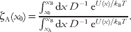
The integrals are dominated by a small region around x=x‡. Hence, ζA(x) is close to 1 from x=x A up to a small distance to the left of x=x‡; it then undergoes a rapid transition to ~1/2 at x=x‡ and to 0 a small distance thereafter. Correspondingly, ρss(x) undergoes a transition from ρeq(x) in the reactant well to 0 in the product well.
When the motion along x is governed by the Langevin equation, ρss(x, v) undergoes a similar transition, along the new coordinate u=λ(x−x‡)−v. The value of ρss(x, v) is ~1/2 at u=0, i.e., on the line v=λ(x−x‡). However, the splitting probability is ~1/2 on the line v=−λ(x−x‡). The sign switch on v is necessary because a molecule starting on the right of x=x‡ must have a leftward velocity for it to have the same splitting probability as a molecule starting at x=x‡ with a zero velocity.
In higher dimensions, the plane on which the splitting probability is 1/2 is known as the stochastic separatrix. Langer's solution to the rate problem shows that the stochastic separatrix is a plane that goes through the saddle point of the energy function; the orientation of the plane is determined by the force-constant matrix at the saddle point and the diffusion or friction matrix. In protein-folding kinetics, the splitting probability is given the name p fold, and the stochastic separatrix is assumed to define the transition-state ensemble (Du et al. Reference Du, Pande, Grosberg, Tanaka and Shakhnovich1998).
3.7 Jump dynamics among discrete microstates
We now further consider the case where motion in the conformational space of a reactant molecule is represented by jumps among a set of discrete microstates. The occupational probabilities, ρi(t), are governed by a master equation:

where kji is the jump rate from microstate i to microstate j. The equilibrium distribution, ρi eq, is determined by the configurational integrals of the microstates. The jump rates satisfy the detailed balance condition:

In particular, master equations have been used to model protein-folding kinetics. In earlier work, the jump rates were made up, only constrained by the detailed balance condition (Alm et al. Reference Alm, Morozov, Kortemme and Baker2002; Cieplak et al. Reference Cieplak, Henkel, Karbowski and Banavar1998; Merlo et al. Reference Merlo, Dill and Weikl2005; Muñoz et al. Reference Muñoz, Henry, Hofrichter and Eaton1998; Schonbrun & Dill, Reference Schonbrun and Dill2003; Weikl et al. Reference Weikl, Palassini and Dill2004; Zwanzig, Reference Zwanzig1995); in more recent work (Buchete & Hummer, Reference Buchete and Hummer2008; Hummer & Kevrekidis, Reference Hummer and Kevrekidis2003), the jump rates are calculated from relatively short simulations of transitions between neighboring microstates [a similar idea is behind the so-called Markov state models (Chodera et al. Reference Chodera, Swope, Pitera and Dill2006, Reference Chodera, Singhal, Pande, Dill and Swope2007; Noe & Fischer, Reference Noe and Fischer2008)]. In matrix–vector form, Eq. (3.106) is

The jump matrix k has one zero eigenvalue, with ρeq as the corresponding eigenvector. The other eigenvalues, λl, l=1, 2, …, are positive; let λl be ordered from small to large.
Now suppose that the microstates are grouped into two states, A and B. When λ1≪λl for all l>1, the transitions between the two states can be modeled well as rate processes, and the rate constants, k ±, are given by

The equilibrium occupational probabilities of the two states are

Instead of solving the eigenvalue problem, one can make a transition-state theory-type estimate for k ±; the presentation below follows the work of Zhou (Reference Zhou2008). As indicated by the derivation in subsubsection 3.1.1, a transition-state theory estimates k + by the normalized total reaction flux from state A to state B, assuming that the occupation of the microstates in state A is according to the equilibrium distribution. That is,
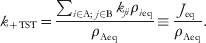
Equation (2.13b) presented in subsection 2.1 can be viewed as a special case of Eq. (3.111). As the discussion of subsubsection 3.5.2 makes it clear, Eq. (3.111) becomes exact in the limit that intra-state equilibration is much faster than inter-state transition.
Like in the continuous case, k +TST provides an upper bound for the rate constant, as has been shown explicitly. In the spirit of variational transition-state theory, one may therefore try to find the best k +TST by varying the dividing surface between the reactant and product states. Here the dividing surface consists of all the allowed jumps (those with non-zero jump rates) between the reactant and product microstates. The optimal dividing surface is the one that minimizes the normalized reaction flux [Eq. (3.111)] and is hence referred to as the minimum-reaction-flux surface. [Note that, as recognized by Krivov & Karplus (Reference Krivov and Karplus2002), locating this surface is isomorphic to the minimum-cut problem in graph theory (Stoer & Wagner, Reference Stoer and Wagner1997).] Test against numerical solutions of master-equation models of protein folding shows that that the minimum-reaction-flux results work well. The minimum-reaction-flux surface separates microstates with large differences in p fold and can be considered as constituting the transition-state ensemble in the discrete case. Among the forward jumps contributing to the minimum reaction flux, one can further identify the one(s) making the largest contribution as the ‘saddle point.’ However, the minimum-reaction-flux approach differs from traditional transition-state theory in one important respect: the dividing surface minimizing the normalized reaction flux is determined not only by the free energies of the microstates (as reflected by ρi eq) but also by the jump rates kji. In principle, dynamic information incorporated by the jump rates can lead to a dominant transition route (or minimum-resistance path) very different from that produced by the free-energy landscape alone. This situation is reminiscent of the continuous case with a position-dependent diffusion coefficient (subsubsection 3.5.1).
4. Bimolecular reactions
Compared to the developments in unimolecular reactions, theories of bimolecular reactions have received much less attention. Often, results for unimolecular reactions are blindly used for bimolecular reactions. A fundamental difference between these two types of reactions is that, in the latter, two reactant molecules have to come into contact with appropriate relative orientations before the reaction can proceed. This intermediate, with near-native separations and relative orientations but without all the short-range native interactions between the reactant molecules, has been referred to as the transient complex (Alsallaq & Zhou, Reference Alsallaq and Zhou2008; Qin & Zhou, Reference Qin and Zhou2008; Zhou et al. Reference Zhou, Wong and Vijayakumar1997). For bimolecular reactions between biomolecules, the overall translation and overall rotation that result in the formation of the transient complex are well modeled as diffusive. From the transient complex, formation of the native complex is essentially a unimolecular process, which proceeds through conformational rearrangement and, along the way, passes through a high-energy transition state. It is important to recognize that both the diffusional process that leads to the transient complex and the conformational rearrangement that finally leads to the native complex can be rate limiting. These are referred to as diffusion controlled and activation controlled, respectively.
To be concrete, we use the binding of a protein and a ligand as our model bimolecular reaction. The reaction path outlined above is captured by the following scheme:
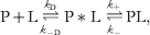
where P∗L denotes the transient complex. Assuming that the transient complex is in steady state, the overall association rate constant is
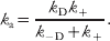
For the sake of completeness, the dissociation rate constant is
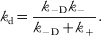
When k +≫k −D, Eq. (4.2a) becomes

resulting in the diffusion-controlled regime. Conversely, when k +≪k −D, Eq. (4.2a) becomes

resulting in the activation-controlled regime. The last expression, in which  is the association constant for the transient complex, indicates that, in the activation-controlled regime, calculating the association rate constant mostly entails dealing with a unimolecular reaction (i.e., k +). The theories of the last section would indicate that, to calculate k +, one has to treat short-range interactions between the protein and the ligand as well as their conformational rearrangements. Given the considerable difficulty and uncertainty, such treatment will be avoided as much as possible, and the focus of this section will be on the diffusion-controlled regime. In terms of the diffusion-controlled rate constant k D and the activation-controlled rate constant k A, the overall association rate constant of Eq. (4.2a) can be expressed as

A simple model for the protein–ligand binding has a centrosymmetric interaction-energy function illustrated in Fig. 4a. Throughout this section, the interaction energy is chosen to be zero when the reactant molecules are far apart. As the two reactant molecules approach each other, they experience electrostatic attraction at long range. At an intermediate distance r=R, the transient complex is formed. Further compaction of the protein–ligand pair encounters an energy barrier (at r=r‡). Crossing this energy barrier leads to a deep energy well, around r=a, which defines the native complex. In particular, in protein–protein association, the energy barrier may come about because side chains in the unbound proteins adopt rotamers different from those in the native complex. Different rotamers are separated by energy barriers; these are amplified by steric hindrance that interfacial side chains experience while the transient complex is transformed into the native complex. If the reactant molecules are assumed to adopt their ‘native’ conformations, i.e., those in the native complex, then the energy barrier would largely disappear, leading to a smoothed energy surface (Alsallaq & Zhou, Reference Alsallaq and Zhou2007a) (Fig. 4a). As we emphasize below, the centrosymmetric model, although useful for illustrating the binding process, suffers from a major limitation. The native complex in this model is constrained only by the distance between the reactant molecules and not by their relative orientations. In contrast, complexes of biological interest are almost always stereospecific. A smoothed interaction-energy function that depends on the separation (represented by r) and relative orientation (represented by Ω) is illustrated in Fig. 4b.
Interaction energy functions. (a) Centrosymmetric model. The solid curve shows the energy function, with locations of the unbound state (i.e., P+L), transient complex (i.e., P*L), transition state, and native complex (i.e., PL) identified. The dashed curve is after smoothing out the transition state. (b) A smoothed energy function in relative translational (r) and rotational (Ω) space. The native complex is located in the deep well; the transient complex is located at the outer boundary of the energy well.

Below we use the centrosymmetric model to introduce basic concepts and then present results for more realistic binding models. The general strategy is to explicitly model the overall translation and overall rotation of the reactant molecules as diffusion, and treat the barrier crossing into the native-complex energy well implicitly, as a unimolecular rate process (in the spirit of the Agmon–Hopfield model). We proceed by first assuming that the reactant molecules are frozen in their native conformations during the diffusional process and then examining the influence of conformational fluctuations.
Throughout this section, we highlight and exploit connections between bimolecular and unimolecular rate constants. The connection is especially direct when protein–ligand binding occurs intramolecularly. For the most part, this section is presented as though the binding is irreversible, but at the end of the section we discuss the kinetics of reversible diffusion-influenced binding.
4.1 Formulation based on dissociation
One approach to calculate the association rate constant k a is to first obtain the rate constant k d for dissociation, which, as noted in subsection 2.2, is a unimolecular reaction, and then find k a as the product of k d and the association constant K a [Eq. (2.17)] (Zhou, Reference Zhou2005a). This requires modeling the motion of the reactant pair in the native-complex energy well. To support results later in this section, here we model motion in the inner well and over the energy barrier as diffusive. We arrive at four useful results. The first is a clarification of the absorbing boundary condition usually used in modeling the diffusion-controlled regime. The second is a demonstration that, in a complete theory, the choice for the location of the transient complex does not affect the overall association rate constant. The third is a clarification of the reactivity that appears in the radiation boundary condition to account for a finite rate constant (i.e., k +) for barrier crossing into the native-complex energy well. The last is an expression for k a based on a time integral.
The probability density in r, ρ(r, t), is assumed to satisfy the three-dimensional Smoluchowski equation

for the full range of the intermolecular distance r; here D is the diffusion constant for relative translation. Because of the centrosymmetry, the problem is effectively one dimensional, i.e., along r; the effect of the other two degrees of freedom is captured by the geometric factor 4πr 2. We apply Kramers' result, Eq. (3.44), to obtain the dissociation rate constant. Setting the limits of the two integrals requires some care. One integral is over the range of the reactant state, which in the present case is the bound state; the lower limit is obviously r=0, and we choose the upper limit to be the top of the energy barrier, i.e., r=r‡. The other integral is from the bottom of the reactant well to the bottom of the product well; the lower limit is obviously r=a, and we choose the upper limit to be at infinite distance, since only then the reactant molecules are fully dissociated. The dissociation rate constant is thus

where we have appropriately inserted the geometric factor 4πr 2.
The association constant for the present model is (Shoup & Szabo, Reference Shoup and Szabo1982; Zhou & Gilson, Reference Zhou and Gilson2009)
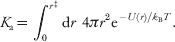
Therefore, the association rate constant is

This result is identical to what Debye (Reference Debye1942) found by imposing an absorbing boundary condition at r=a (see subsubsection 4.3.1). In the above derivation, there is no absorbing boundary condition at r=a; rather, a deep well is there. Therefore, the absorbing boundary condition used in modeling the diffusion-controlled regime corresponds to a deep and narrow energy well in front of a reflecting wall. This is the first main result of this subsection.
Note that the location of the transient complex does not appear in the expression for k a. To make connection with the overall association rate constant given by Eq. (4.4), we write Eq. (4.8) as

The numerator of the first term can be identified with the inverse of the rate constant k + of unimolecular transition to the native complex from the transient complex. The transient complex here is confined to the narrow region between r‡ and r‡+Δ (>R), with the latter serving as a reflecting boundary for the transient complex. The denominator of the first term can be identified with the association constant,  , for the transient complex [cf. Eq. (4.7)]. The second term can be recognized as the diffusion-controlled rate constant, obtained by imposing an absorbing boundary condition at r=R:

Thus,
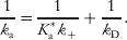
This shows that k a given by Eq. (4.8) can be written in the form of Eq. (4.4). Had we started with Eq. (4.4) and calculated the diffusion-controlled rate constant k D and the activation-controlled rate constant k A, we would have ended up with Eq. (4.8) as the final result for k a, which, as noted above, is independent of the location of the transient complex. This demonstrates that, in a complete theory, the choice for the location of the transient complex does not affect the overall association rate constant.
Equation (4.10a) for k a can be further written in a form obtained by imposing the radiation boundary condition of Collins & Kimball (Reference Collins and Kimball1949) at r=R (Shoup & Szabo, Reference Shoup and Szabo1982):

Compared with the Collins–Kimball result [Eq. (4.18)], we find that the reactivity κ in the radiation boundary condition [Eq. (4.15a)] can be identified with k +Δ. Hence, κ is a way to implicitly model the transition from the transient complex to the native complex. This is the third main result of this subsection.
Finally, we apply the time-integral expression, Eq. (3.30), to find an alternative formula for the dissociation rate constant. In the present case, the ratio of the equilibrium occupation probabilities is
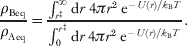
Note that the integral in the numerator essentially is the volume V of the container and is effectively infinite relative to the integral of the denominator. Hence ρAeq→0 and ρBeq→1. Equation (3.30) specialized to the present case is thus

where ρN(r, t | r0) is the conditional probability density satisfying natural boundary conditions. Combined with the equilibrium constant of Eq. (4.7), we arrive at the following expression for the association rate constant:

Using the conditional probability density to evaluate the above expression, we derive Eq. (4.8) as a good approximation for k a when the inner well features a deep minimum. This expression of the rate constant is the last main result of this subsection, which will be further analyzed and extended below.
4.2 Activation-controlled regime: transition-state theory
While our focus is on the diffusion-controlled regime, for the sake of completeness, we mention the association rate constant predicted by the transition-state theory of Eyring (Reference Eyring1935). Corresponding to Eq. (3.31) for the rate constant of a unimolecular reaction, the rate constant for a bimolecular reaction is

where q P and q L are the partition functions of the protein and the ligand, respectively;  is a partition function calculated for a protein–ligand pair without including the reaction coordinate (as signified by the prime), which is fixed at the value defining the transition state; U‡ is the protein–ligand interaction energy in the transition state; and V is the volume of the container.
To illustrate, consider the centrosymmetric model. We calculate the partition functions according to classical statistical mechanics. The protein molecule has only three degrees of freedom, for overall translation. Hence, q P=h −3V(2πk BTm P)3/2, where m P is the mass of the protein. Similarly, q L=h −3V(2πk BTm L)3/2.  involves five degrees of freedom: three for overall translation and two for relative translation orthogonal to r; the masses corresponding to these two types of motions are the total mass, m P+m L, and reduced mass, m Pm L/(m P+m L), respectively. Hence,

The activation-controlled rate constant is finally given by

As to be expected from a classical treatment, Planck's constant disappears from the final result.
4.3 Diffusion-controlled regime
We now explicitly model the overall translational and rotation diffusion of the reactant molecules and implicitly model the barrier crossing into the inner energy well. We show that the overall association rate constant can be written in the form of Eq. (4.4); thereafter, we focus on the diffusion-controlled rate constant k D.
4.3.1 Centrosymmetric model
In the Smoluchowski (Reference Smoluchowski1917) approach to modeling diffusion-influenced bimolecular reactions, one works with the pair distribution function, P(r, t). It satisfies the Smoluchowski equation, Eq. (4.5), with a radiation boundary condition (Collins & Kimball, Reference Collins and Kimball1949)

and a value

The initial value of P(r, t) is

corresponding to an equilibrium distribution. A time-dependent rate coefficient is defined as the total inward flux at r=R:

It can be shown that, if a protein binds irreversibly [as modeled by the radiation boundary condition of Eq. (4.15a)] with a ligand that is in excess, the decay of the protein concentration is governed by (Solc & Stockmayer, Reference Solc and Stockmayer1971; Szabo, Reference Szabo1989)
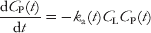
or
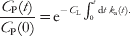
Note that C p(t)/Cp(0) is equivalent to the survival probability of a single protein molecule surrounded by ligand molecules at concentration C L.
The long-time limit, k a(∞), of the rate coefficient introduced here corresponds to the association rate constant of subsection 4.1. We will continue to denote k a(∞) simply as k a. Solving for P(r,∞), one obtains

where k D is the Debye result given by Eq. (4.9). This result for the overall association rate constant, as well as similar results later in this subsection, conforms to Eq. (4.4). As we explained above, the reactivity κ models the transition from the transient complex to the native complex. (When κ=0, the boundary becomes reflecting.) The limit κ→∞ corresponds to the situation where a reactant pair once reaching the transient complex is instantaneously transformed into the native complex. The rate of association is then limited by the relative translational diffusion to reach the transient complex; that is why the rate constant in this limit, k D, is referred to as diffusion controlled. In this limit, the radiation boundary condition reduces to the absorbing boundary condition:

In short, the diffusion-controlled rate constant k D is obtained by setting an absorbing condition at the transient complex. In the opposite limit κ→0, diffusion is able to replenish the reactant pairs lost by forming the native complex, so the initial equilibrium distribution is maintained. Then the steady-state value, k a(∞), is the same as the initial value, k a(0); i.e., the rate constant approaches

which is the activation-controlled limit.
When the interaction potential U(r) is absent, the Debye result [Eq. (4.9)] reduces to the well-known Smoluchowski formula

Throughout this section, we use a superscript ‘0’ to signify a rate constant calculated in the absence of an interaction potential; k D0 is the limit of the rate constant set by random diffusion and is referred to as the basal rate constant. An attractive potential is expected to increase k D. To illustrate, consider a Coulomb interaction potential, U(r)=−Q/r. Evaluating the Debye formula, we find
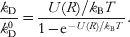
When the value of the potential at contact, U(R), is 9k BT, the electrostatic attraction results in a modest increase of 9-fold in the association rate constant. This result will be contrasted below with much more significant electrostatic rate enhancement predicted from a more realistic model of protein–protein association.
The probability, S(t|r0), that a protein–ligand pair, started at an initial separation r0, has not formed the native complex at time t is known as the survival probability. It is related to the pair distribution function via

and hence satisfies the equation
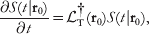
with the boundary conditions


At t=∞, the left-hand side of Eq. (4.24) becomes 0, and the survival probability is called the escape probability. When the boundary at r=R is absorbing, the escape probability is very similar in form to the splitting probability of subsubsection 3.6.2. For the present model one has

which can be compared with the splitting probability given by Eq. (3.105). However, the behaviors of the splitting probability there and the escape probability here are very different. The energy function modeling the unimolecular transition between two states features a barrier, where the splitting probability undergoes a rapid transition from 0 to 1. In contrast, the energy function modeling intermolecular interaction has a longer range and is relatively monotonic; hence, the transition of the escape probability from 0 to 1 is more gradual. When no interaction potential is present, the escape probability is 1−R/r 0.
As we clarified in subsection 4.1, an absorbing boundary is equivalent to a narrow deep energy well in front of a reflecting wall. If the absorbing boundary for calculating k D is replaced by such an energy well, then the time-integral formula, Eq. (4.12), for the association rate constant can be used to calculate k D. We thus have

where Δ, the width of the energy well, approaches zero, and the conditional probability density ρR(r, t|r0) satisfies a reflecting boundary condition at r=R.Footnote 2 From this formula for k D, one can also derive the Debye result [Eq. (4.9)].
4.3.2 Anisotropic reactivity on protein molecule
As we emphasized, protein–ligand native complexes are stereospecific. The ligand binds to a specific site on the protein surface rather than the whole surface; hence, the reactant pair must satisfy constraints in both separation and relative orientation before the native complex can be formed. One then needs to model both relative translational diffusion and rotational diffusion of the reactant molecules. Here we treat the case where the ligand is point-like so that its orientation does not come into play; the case where rotational diffusion of the ligand is also modeled is deferred to the next subsubsection. For simplicity, we assume that the protein molecule is axially symmetric; we denote the axis of symmetric by the unit vector nP. The pair distribution function now depends both on r and on nP, and is denoted as P(r, nP, t). On account of rotational diffusion, the governing equation for P(r, nP, t) is

where P(nP) is a rotational diffusion operator given by

with D P denoting the rotational diffusion constant of the protein molecule. The stereospecific binding site can be modeled by modifying the radiation boundary condition to one that is of the radiation type if the ligand falls inside the site and becomes reflecting otherwise (Solc & Stockmayer, Reference Solc and Stockmayer1971). That is, at r=R,

where  is the unit vector along r, and θ* (, nP) has value 1 if the angle between and nP is within the angle span, δP, of the ‘reactive patch’ and value 0 otherwise.
The boundary condition of Eq. (4.29) is a mixed type (i.e., involving the pair distribution in one part of the boundary and its flux in another), which poses a mathematical challenge. To get around this problem, Shoup et al. (Reference Shoup, Lipari and Szabo1981) introduced an approximation. They assume that the flux is a constant over the reactive patch, and this constant is determined by requiring that Eq. (4.29a) is satisfied only on averaging over the reactive patch, not at every point over it. With this constant-flux approximation, the boundary condition at r=R now becomes

where J (which depends on time for the time-dependent problem) is fixed by requiring

with 〈· · ·〉* denoting an average over the reactive patch. In the absence of an interaction potential, the association rate constant is given by
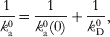
where


In the last two equations, F P=(1−cosδP)/2 is the surface fraction covered by the reactive patch, μl=[l(l+1)D P/D]1/2R, Pl(x) are Legendre polynomials, and (π/2x)1/2Kl +1/2(x) are modified Bessel functions of the third kind. The above result for k a0 was essentially guessed by Solc & Stockmayer (Reference Solc and Stockmayer1973). Berg (Reference Berg1985) found that ΛP/F P can be approximated by

where νP=[(1+D PR 2/D)/2]1/2. When D P→0, Eq. (4.31c) reduces to
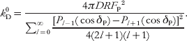
The case of small reactive patches, corresponding to stereospecific binding, is of particular interest. A patch with angle span δP→0 on a spherical surface is equivalent to a disk with radius a=RδP on an infinite reflecting plane. Applying the constant-flux approximation to the latter problem, Shoup et al. found that k D0=(3π2/8)Da (assuming D P=0). This is to be compared with the exact solution of the problem, k D0=4Da (Hill, Reference Hill1975). These results show that the constant-flux approximation underestimates the diffusion-controlled rate constant by ~7% when δP→0. Note that, when δP→0, k D0∝δP, not δP2, as suggested by the surface fraction of the reactive patch. The weaker δp-dependence (and hence higher value) of k D0 comes about due to the diffusive nature of the ligand molecule's motion. When a ligand molecule first reaches the reflecting part of the protein surface, it can come back and try again to reach the reactive patch.
Zhou (Reference Zhou1993) applied the constant-flux approximation to find the rate constant when a Coulomb potential U(r)=−Q/r is present. The result is given by
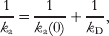
where

When the rotation diffusion constant D P=0, the diffusion-controlled rate constant is

where Q 1=U(R)/2k BT and (π/2x)1/2Il +1/2(x) are modified Bessel functions of the first kind. It was observed that, as δP→0, terms with larger and larger l become dominating in the sum over l; for those terms, the Q 1-dependent factors become less and less important. Therefore, the whole denominator becomes nearly independent of Q 1, and consequently

where k D0 is the basal rate constant of Eq. (4.31e). The generality of Eq. (4.33) for small reactive patches (i.e., stereospecific binding) was recognized. In fact, this approximate formula was first suggested by results obtained by Brownian dynamics simulations, and the above deduction served to confirm the simulation results. Below we further elaborate on the generality of Eq. (4.33) and its use in modeling the effect of long-range electrostatic attraction on stereospecific protein–ligand binding.
4.3.3 Anisotropic reactivity on both protein and ligand molecules: free diffusion
Before we further consider the effect of the interaction potential, we present the more general binding model in which the protein molecule and the ligand molecule each bear a reactive patch, which for now is assumed to be axially symmetric. The pair distribution function, P(r, nP, nL, t), is now governed by

where L(nL) is the diffusion operator for ligand rotation [see Eq. (4.28b)]. The boundary condition at r=R becomes (Solc & Stockmayer, Reference Solc and Stockmayer1971)

where θ* (, nP, nL) has value 1 if the angles between and nP and between and nL are within the angle spans, δP and δL, of the respective reactive patches, and value 0 otherwise.
The rate constant for the one-patch model in the absence of an interaction potential is given by Eqs. (4.31a–c). To derive k a0 for the present two-patch model, Solc & Stockmayer (Reference Solc and Stockmayer1973) first devised a reaction scheme for the one-patch model. The scheme involves two intermediates, in which the ligand is in contact with the reflecting part of the protein and with the reactive patch, respectively. The overall rate constant of this scheme was compared to Eqs. (4.31a–c) to identify the individual rate constants in the scheme. They then extended this scheme to the two-patch model, now involving four intermediates. The expression for k a0 via this ‘quasi-chemical’ scheme for the two-patch model can again be written in the form of Eq. (4.31a), but now

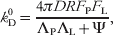
where

with ΛP defined by Eq. (4.31c) and ΛL defined analogously. For small patches, using Eq. (4.31d) for ΛP and a similar approximation for ΛL and keeping the lowest orders, one finds (Berg, Reference Berg1985)

This result shows that, when δP and δL→0, k D0∝δP2δL~δPδL2, not δP2δL2, as suggested by the surface fractions of the reactive patches. Again, k D0 is higher than expected from surface fractions because the diffusive nature of its motion allows the reactant pair to make repeated attempts to reach the absorbing boundary.
By applying the constant-flux approximation, Zhou (Reference Zhou1993) solved the diffusion equation for the two-patch model to find the time-dependent rate coefficient k a0 (t). The result, in Laplace transform, is given by
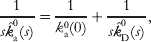
where k a0 (0) is given by Eq. (4.36a). Note that the long-time limit of k a0 (t) is given by the s→0 limit of s  a0 (s) and similarly for k D0. The basal rate coefficient is

where  and
 is expressed in terms of Wigner's 3-j symbols:

The one-patch model is a special case with δL=π. In that case the only term in the summation over l 2 is l 2=0; it can be verified that the s→0 limit of Eq. (4.37b) reduces to Eq. (4.31c) of the one-patch model. Numerically, the results for the basal rate constant by the quasi-chemical scheme and by the constant-flux approximation are very close.
A third solution for the basal rate constant was obtained by Temkin & Yakobson (Reference Temkin and Yakobson1984), using a formula obtained by Doi (Reference Doi1975a, Reference Doib). Inspired by the closure approximation of Wilemski & Fixman (Reference Wilemski and Fixman1973), Doi derived a variational formula for the basal rate constant. With the simplest trial function, the basal rate constant for the present case takes the form

where, for notational simplicity, we have written (r, nP, nL) collectively as x, and ρR0 (x, t|x0) is the conditional probability for free diffusion subject to a reflecting boundary condition at r=R. It can be recognized that Eq. (4.38) is a generalization of the time-integral formula of Eq. (4.27). Temkin and Yakobson's solution entailed finding the conditional probability and evaluating the integrals. The final result is identical to the s→0 limit of Eq. (4.37b), suggesting that the time-integral formula and the constant-flux approximation are equivalent. This equivalence was proven by Zhou & Szabo (Reference Zhou and Szabo1996a); see subsubsection 4.3.5.
The two-patch model was taken to its limit when the restriction on axial symmetry of the reactive patches was removed (Schlosshauer & Baker, Reference Schlosshauer and Baker2002). Now, for each reactant molecule, one additional rotational degree of freedom, i.e., rotation angle χP or χL around the unit vector nP or nL, needs to be accounted for. Using the constant-flux approximation, Schlosshauer and Baker were able to obtain the basal rate constant.
4.3.4 Anisotropic reactivity on both protein and ligand molecules: effect of interaction potential
Zhou (Reference Zhou1993) treated the two-patch model when a centrosymmetric interaction potential, U(r), is present. Applying the constant-flux approximation, he found
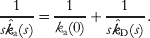
The initial rate coefficient is

The diffusion-controlled rate coefficient is

where a prime signifies a derivative with respect to r, and f l(r; μ) is a function that satisfies

and decays to zero as r→∞. When U(r)=0, Eq. (4.39c) reduces to Eq. (4.37b).
While no solution of Eq. (4.39d) could be found for an arbitrary U(r), Zhou (Reference Zhou1997) was able to solve Eq. (4.39d) for two potential functions: a square-well potential and U(r)=−2k BT ln[1+(exp(−U(R)/2k BT)−1)R/r]. A main aim for finding explicit results of k D for these potentials is to demonstrate the accuracy of the simple formula given by Eq. (4.33) for small patches. For example, at δP=δL=5°, the prediction of Eq. (4.33) overestimates the result given by Eq. (4.39c) for the logarithmic potential by merely 5% when U(R)=−9k BT. The rate enhancement,  , by this potential is ~8000. This dramatic rate enhancement is to be contrasted with the modest result of subsubsection 4.3.1 for the case where the reactant molecules have isotropic reactivity.
4.3.5 Generalization of Eq. (4.33)
Equation (4.33) presents an enormous simplification for accounting for the effect of interaction potentials on association rate constant. The individual results summarized above suggest that it is quite general for stereospecific binding. A general form of Eq. (4.33) was established through a pair of papers in 1996.
In the first paper, Zhou & Szabo (Reference Zhou and Szabo1996a) considered a general binding model in which the relative translational and overall rotational degrees of freedom of the reactant pair are collectively denoted as x. The transition from the transient complex to the native complex was modeled not by a radiation or absorbing boundary condition. Rather, the transient complex was assumed to be confined to a ‘reactive region’ in x space, specified by the function θ*(x) with value 1 in the reactive region and value 0 elsewhere. From the reactive region, the reactant pair forms the native complex with a rate constant k +. The governing equation for the pair distribution function is

where (x) is an operator modeling the diffusional motion of the reactant pair. This model is similar in spirit to the Agmon–Hopfield model [see Eq. (3.89)]; it can also be viewed as a microscopic implementation of reaction scheme (4.1). Because the transition from the transient complex to the native complex is accounted for by the reaction term in Eq. (4.40), the inner boundary is reflecting. The rate coefficient is given by

When the reactive region spans a patch on the inner boundary and a thickness Δ→0 in the normal direction, then the sink term in Eq. (4.40) is equivalent to a radiation boundary condition on the reactive patch, with κ given by k +Δ (which uncoincidentally is consistent with the discussion of subsection 4.1). The constant-flux approximation is derived when the pair distribution is assumed to follow the equilibrium distribution, P eq(x)∝exp[−U(x)/k BT], but with a time-dependent magnitude. Then it was shown that the rate coefficient can again be written as Eq. (4.39a), with


where 〈· · ·〉* denotes an average over the reactive region [the last step of Eq. (4.42a) applies to a small reactive region], and ρR (x, t | x0) is the conditional probability satisfying

subject to a reflecting condition on the inner boundary. Equation (4.42b) reduces to the time-integral formulas for rate constants presented above in this subsection under different situations, including Eq. (4.38) for the two-patch model.
In a subsequent paper (Zhou, Reference Zhou1996), it was noted that, when the interaction potential U(x) is long ranged so that it is almost constant in the reactive region and its vicinity, then ρR (x, t | x0) is almost independent of the potential, i.e., ρR (x, t | x0)≈ρR0 (x, t | x0), for x and x0 both inside the reactive region. Consequently,
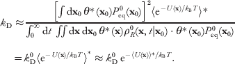
This is finally the general result that provides a powerful method for modeling the effect of long-range electrostatic attraction on stereospecific protein–ligand binding.
That a small reactive region is necessary for the validity of Eq. (4.44) can be demonstrated by the Debye result for the centrosymmetric model, in which the native complex has no requirement on relative orientation. In particular, Eq. (4.22), the Debye result for a Coulombic potential, shows a very different dependence on the potential than Eq. (4.44). As noted above, the rate enhancement given by Eq. (4.22) is much more modest than would be predicted by Eq. (4.44).
To complete the connection with reaction scheme (4.1), we note that the association constant for the transient complex is
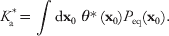
Combined with k D given by Eq. (4.42b), we find that the rate constant for dissociating the transient complex by diffusion is

The last result could also be derived from a time-integral formula, Eq. (3.88), of section 3. The right-hand side can be recognized as the mean residence time in the reactive region, which measures how long it takes for ligand molecules to move out of the reactive region via diffusion (while the pathway to form the native complex is turned off). The above derivation of Eq. (4.44) is the same as proving that the mean residence time is nearly independent of the long-range interaction potential. As observed by Zhou et al. (Reference Zhou, Wong and Vijayakumar1997), the smaller the reactive region, the faster the ligand population in it will decay, and hence the shorter the mean residence time. If the mean residence time is really short, then the ligand molecules that have diffused out will not move very far away. Now if the interaction potential does not vary significantly in the reactive region and its vicinity, then the ligand molecules would have moved in an essentially uniform potential. Consequently, k −D would be nearly the same as if the potential is absent.Footnote 3
4.3.6 Atomistic models: transient-complex theory
The derivation of Eq. (4.44) makes it clear that its validity is subject to the condition that the reactive region is small while the interaction potential is long ranged. This condition is exactly met (fortuitously) for stereospecific protein–ligand binding under the influence of electrostatic attraction. The accuracy of Eq. (4.44) for atomistic protein–ligand models has been demonstrated by comparison against Brownian dynamics simulations (Zhou et al. Reference Zhou, Briggs and Mccammon1996, Reference Zhou, Wong and Vijayakumar1997, Reference Zhou, Briggs, Tara and Mccammon1998a).
The dependence of the diffusion-controlled rate constant on interaction potential given by Eq. (4.44) has an Arrhenius appearance. Such a dependence is expected for the activation-controlled rate constant k A [see, e.g., Eq. (4.42a)], but totally unexpected for k D [see, e.g., Eq. (4.22)]. Despite the Arrhenius appearance, k D does not model an activation process.Footnote 4 The average interaction energy of the transient complex, 〈U〉*, which superficially resembles the activation energy in Eyring's and Kramers' theories, is typically negative (leading to rate enhancement) instead of being positive. Unlike the processes studied by Eyring and Kramers, where an energy barrier is what hinders the rate, the diffusion-controlled rate of protein–ligand binding is hindered by the translational and rotational constraints of the transient complex.
To calculate k D, the transient complex has to be specified. Rather than being guided by any theoretical considerations, for many years the location of the transient complex (or, its equivalence in the form of an absorbing boundary) was proposed in an ad hoc way and often adjusted for best agreement with experiment (Altobelli & Subramaniam, Reference Altobelli and Subramaniam2000; Elcock et al. Reference Elcock, Gabdoulline, Wade and Mccammon1999; Gabdoulline & Wade, Reference Gabdoulline and Wade1997, Reference Gabdoulline and Wade2001; Gabdoulline et al. Reference Gabdoulline, Kummer, Olsen and Wade2003; Miyashita et al. Reference Miyashita, Onuchic and Okamura2004; Northrup & Erickson, Reference Northrup and Erickson1992; Northrup et al. Reference Northrup, Reynolds, Miller, Forrest and Boles1986; Spaar et al. Reference Spaar, Dammer, Gabdoulline, Wade and Helms2006; Vijayakumar et al. Reference Vijayakumar, Wong, Schreiber, Fersht, Szabo and Zhou1998; Zhou, Reference Zhou1993; Zhou et al. Reference Zhou, Briggs and Mccammon1996, Reference Zhou, Wong and Vijayakumar1997, Reference Zhou, Briggs, Tara and Mccammon1998a). In order to predict association rate constants from theory alone, the transient complex has to be specified without reference to experiment. The problem is especially challenging for protein–protein association, given the severity of orientational constraints on both reactant molecules. A solution was proposed by Alsallaq and Zhou (Alsallaq & Zhou, Reference Alsallaq and Zhou2007a), based on analyzing the interaction energy landscape of associating proteins.
As discussed in subsection 4.1, in a complete theory, the overall association rate constant k a should not be sensitive to where the transient complex is placed. If it is placed far away from the native complex, then k D will be large but k + will be small. Conversely, if it is placed very close to the native complex, then k D will be reduced but k + will become very large. Either way, Eq. (4.4) is expected to give nearly the same result for k a. However, given the considerable difficulty and uncertainty in the calculation of k +, it is highly desirable to use k D as a close approximation for k a. Then there is an optimal location for placing the transient complex (Zhou, Reference Zhou2001a). If it is placed too far from the native complex, then the resulting k D would not be a useful approximation for k a. On the other hand, placing the transient complex too close to the native complex would mean that short-range interactions and conformational rearrangement have to be dealt with in calculating k D. The native complex sits in a deep well in the interaction energy landscape. The optimal placement for the transient-complex ensemble is at the outer boundary of the native-complex energy well (Alsallaq & Zhou, Reference Alsallaq and Zhou2007a; Zhou, Reference Zhou2001a) (Fig. 4b).
The algorithm for identifying the transient complex was based on the following observation: inside the native-complex energy well, translation and rotation are restricted, but, once outside, the proteins gain significant translational and rotational freedom (Zhou, Reference Zhou2001a) (Fig. 5a). Thus, the outer boundary of the native-complex energy well coincides with the onset of translational and rotational freedom. To simplify the calculations required for determining the transient complex, the short-range interaction energy stabilizing the native complex was modeled by the number of contacts, N c, formed between the protein partners. Translational and rotational freedom was measured by σχ(N c), the standard deviation of the rotation angle χ in configurations with a given contact level N c. A sharp increase in σχ with decreasing N c marks the onset of translational and rotational freedom and hence the location of the transition complex (Fig. 5b).
Specification of the transient complex for the barnase–barstar protein pair (Alsallaq & Zhou, Reference Alsallaq and Zhou2008). (a) Scatter plot of allowed (i.e., clash-free) configurations. Each scatter point represents a cluster of allowed configurations with the indicated contact number (N c) and angle (χ) of relative rotation. The N c level defining the transient complex is shown in dark color. (b) Transition of the standard deviation of χ, σχ, from the native complex (with high contact numbers) to the unbound state (with low contact numbers). The start of the sharp increase in σχ, as indicated by an arrow, marks the transient complex.

Since k D is used as the prediction for k a, Eq. (4.44) can be rewritten as an equation for k a:

where k a0 now denotes the basal rate constant, i.e., the rate constant for reaching the transient complex by translational and rotational diffusion in the absence of any biasing force, and the interaction potential is denoted with a subscript ‘el’ to signify that only electrostatic interactions are to be included. The neglect of short-ranged non-electrostatic effects from the Boltzmann factor is based on two considerations. First, transient-complex configurations are separated by at least one layer of solvent (Alsallaq & Zhou, Reference Alsallaq and Zhou2007b, Reference Alsallaq and Zhou2008); therefore, short-ranged forces such as hydrophobic and van der Waals interactions are relatively weak in the diffusion process, leading to the transient complex. Second, short-range interactions, even when present within the transient complex, contribute much less to rate enhancement (i.e., k a/k a0) compared to long-range interactions (see next subsubsection). However, short-range interactions are essential for determining the location and size of the transient-complex ensemble in configurational space, which in turn affect the magnitude of k a0. A transient-complex ensemble that is less restricted in translation and rotation will lead to a higher k a0.
The algorithm for identifying the transient-complex ensemble presented above along with Eq. (4.46) constitutes the transient-complex theory. The theory provides an interesting dissection on the wide spectrum of observed rate constants of protein–protein association (Alsallaq & Zhou, Reference Alsallaq and Zhou2008). Brownian dynamics simulations have found that basal rate constants, set by unbiased diffusion, are in the range of 104–106 M−1 s−1 (Alsallaq & Zhou, Reference Alsallaq and Zhou2008; Qin & Zhou, Reference Qin and Zhou2009). This is the range of rate constants observed on antibody–antigen binding (Foote & Eisen, Reference Foote and Eisen1995; Hoffman et al. Reference Hoffman, Labranche, Zhang, Canziani, Robinson, Chaiken, Hoxie and Doms1999; Wassaf et al. Reference Wassaf, Kuang, Kopacz, Wu, Nguyen, Toews, Cosic, Jacques, Wiltshire, Lambert, Pazmany, Hogan, Ladner, Nixon and Sexton2006); presumably, antibodies are not specifically optimized for fast binding, and antibody–antigen binding processes are described well as unbiased diffusion. However, many proteins are observed to associate faster than the basal rate constant (Baerga-Ortiz et al. Reference Baerga-Ortiz, Rezaie and Komives2000; Candia et al. Reference Candia, Garcia and Latorre1992; Darling et al. Reference Darling, Kuchibhotla, Glaesner, Micanovic, Witcher and Beals2002; Escobar et al. Reference Escobar, Root and Mackinnon1993; Gianni et al. Reference Gianni, Engstrom, Larsson, Calosci, Malatesta, Eklund, Ngang, Travaglini-Allocatelli and Jemth2005; Goldstein & Miller, Reference Goldstein and Miller1993; Hemsath et al. Reference Hemsath, Dvorsky, Fiegen, Carlier and Ahmadian2005; Johnson et al. Reference Johnson, Mccoy, Bingman, Phillips and Raines2007; Korennykh et al. Reference Korennykh, Piccirilli and Correll2006; Miller, Reference Miller1990; Murrell-Lagnado & Aldrich, Reference Murrell-Lagnado and Aldrich1993; Park & Raines, Reference Park and Raines2001; Radic et al. Reference Radic, Kirchhoff, Quinn, Mccammon and Taylor1997; Schreiber & Fersht, Reference Schreiber and Fersht1996; Shapiro et al. Reference Shapiro, Ruiz-Gutierrez and Chen2000; Shen et al. Reference Shen, Hage and Sebald1996; Stewart & Van Bruggen, Reference Stewart and Van Bruggen2004; Terlau et al. Reference Terlau, Shon, Grilley, Stocker, Stuhmer and Baldomero1996; Uter et al. Reference Uter, Gruic-Sovulj and Perona2005; Walker et al. Reference Walker, Moore, James and Kleanthous2003; Wallis et al. Reference Wallis, Moore, James and Kleanthous1995; Wendt et al. Reference Wendt, Leder, Harma, Jelesarov, Baici and Bosshard1997). These association rate constants must have been enhanced by a biasing force. The electrostatic surfaces of the reactant partners in these systems indeed show complementarity (Alsallaq & Zhou, Reference Alsallaq and Zhou2008; Schreiber et al. Reference Schreiber, Haran and Zhou2009), indicating that electrostatic attraction provides the rate enhancement. The transient-complex theory suggests that the narrow range of 104–106 M−1 s−1 serves as a demarcation: lower rate constants implicate activation control, whereas rate constants in this range and higher implicate diffusion control, with the higher rate constants further implicating electrostatic attraction.
As recognized previously (Zhou, Reference Zhou2001a, Reference Zhou2003a), the transient-complex theory provides a nice explanation for a widely observed phenomenon regarding the effects of ionic strength on protein association kinetics. For many protein complexes that apparently are under diffusion control, the association and dissociation rate constants show disparate dependences on ionic strength: k a decreases significantly with increasing ionic strength, whereas k d is only modestly affected by ionic strength (Baerga-Ortiz et al. Reference Baerga-Ortiz, Rezaie and Komives2000; Candia et al. Reference Candia, Garcia and Latorre1992; Darling et al. Reference Darling, Kuchibhotla, Glaesner, Micanovic, Witcher and Beals2002; Escobar et al. Reference Escobar, Root and Mackinnon1993; Gianni et al. Reference Gianni, Engstrom, Larsson, Calosci, Malatesta, Eklund, Ngang, Travaglini-Allocatelli and Jemth2005; Goldstein & Miller, Reference Goldstein and Miller1993; Hemsath et al. Reference Hemsath, Dvorsky, Fiegen, Carlier and Ahmadian2005; Miller, Reference Miller1990; Murrell-Lagnado & Aldrich, Reference Murrell-Lagnado and Aldrich1993; Radic et al. Reference Radic, Kirchhoff, Quinn, Mccammon and Taylor1997; Schreiber & Fersht, Reference Schreiber and Fersht1993; Shen et al. Reference Shen, Hage and Sebald1996; Stewart & Van Bruggen, Reference Stewart and Van Bruggen2004; Walker et al. Reference Walker, Moore, James and Kleanthous2003; Wallis et al. Reference Wallis, Moore, James and Kleanthous1995; Wendt et al. Reference Wendt, Leder, Harma, Jelesarov, Baici and Bosshard1997). Ionic strength serves to modulate the magnitude of the electrostatic attraction between two proteins; the attraction is weakened when ionic strength is increased, leading to significant decrease in k a. Under diffusion control, k d≈(k −/k +)k −D [Eq. (4.2b)]; neither k −D nor k −/k + has much dependence on ionic strength. The former is because k −D does not depend much at all on the electrostatic attraction (see preceding subsubsection). The latter comes about because of the close proximity of the transient and the native complexes; then ionic strength modulates electrostatic interactions in them to similar extents and consequently has little effect on their equilibrium constant k −/k +.
Quantitative test against experimental data on many protein–protein and protein–RNA complexes (Law et al. Reference Law, Linde, Chambers, Oubridge, Katsamba, Nilsson, Haworth and Laird-Offringa2006; Radic et al. Reference Radic, Kirchhoff, Quinn, Mccammon and Taylor1997; Schreiber & Fersht, Reference Schreiber and Fersht1993, Reference Schreiber and Fersht1996; Shen et al. Reference Shen, Hage and Sebald1996; Wallis et al. Reference Wallis, Moore, James and Kleanthous1995) has clearly demonstrated the predictive power of the transient-complex theory (Alsallaq & Zhou, Reference Alsallaq and Zhou2007b, Reference Alsallaq and Zhou2008; Qin & Zhou, Reference Qin and Zhou2008). In a recent study, the theory was used to dissect a record-setting rate constant, at >1010 M−1 s−1 (Korennykh et al. Reference Korennykh, Piccirilli and Correll2006), of a ribotoxin binding to a biologically essential RNA loop on the ribosome (Qin & Zhou, Reference Qin and Zhou2009). Electrostatic attraction provides a 5×10⁶-fold rate enhancement. In comparison, the binding rate constant to the isolated RNA loop is electrostatically enhanced by 5×10²-fold, in line with the results found in other protein–protein and protein–RNA complexes (Alsallaq & Zhou, Reference Alsallaq and Zhou2007b, Reference Alsallaq and Zhou2008; Qin & Zhou, Reference Qin and Zhou2008). There are two contributions to the additional 104-fold rate enhancement. First, the rest of the ribosome provides extra electrostatic attraction to the ribotoxin. Second, neighboring ribosomal proteins reshape the binding interface to position the transient complex into a region in configurational space where the electrostatic attraction between the ribotoxin and the RNA loop is particularly strong.
4.3.7 Facilitation by non-specific binding
A biological problem of great interest is the search by DNA-binding proteins for specific sites on genomic DNA. This potentially is a slow process, akin to finding a needle (i.e., a specific site) in a haystack (i.e., genomic DNA). That it is completed in short times routinely in cells prompted Adam & Delbruck (Reference Adam, Delbruck and Davidson1968) to look for an explanation. Their key observation is that, by non-specifically binding to the DNA surface, a protein searches for a specific site in a one-dimensional space rather than three-dimensional spaces. The search time, as their calculations of first mean passage time show, in the lower dimensionality is significantly shorter. This reduction of dimensionality idea has been further developed (Berg et al. Reference Berg, Winter and Von Hippel1981; Berg & Ehrenberg, Reference Berg and Ehrenberg1982; Halford & Marko, Reference Halford and Marko2004; Richter & Eigen, Reference Richter and Eigen1974; Riggs et al. Reference Riggs, Bourgeois and Cohn1970; Schranner & Richter, Reference Schranner and Richter1978). In particular, Berg et al. (Reference Berg, Winter and Von Hippel1981) phenomenologically described four modes of non-specific binding-facilitated translocation along the DNA: sliding, hopping, jumping, and intersegment transfer. Berg & Ehrenberg (Reference Berg and Ehrenberg1982) empirically incorporated diffusion on the DNA surface, or surface diffusion, into the Smoluchowski approach to diffusion-influenced reactions.
Zhou & Szabo (Reference Zhou and Szabo2004) introduced a more fundamental and realistic treatment, in which non-specific binding is accounted for by a short-range attractive potential around the DNA surface. The first three modes described by Berg et al. (Reference Berg, Winter and Von Hippel1981) are all encompassed in this treatment and there is no need (and rigorously it is impossible) to distinguish them. (The fourth mode, intersegment transfer, applies to bivalent proteins and is not dealt with in this work.) Zhou and Szabo modeled the protein as an isotropically reactive sphere, the DNA as an infinite cylinder (with contact distance R), and the specific binding site as a reactive strip (with height 2η); the short-range attractive potential, U(r), was assumed to be axially symmetric (r here denotes distance to the cylinder axis). Applying the constant-flux approximation, the rate coefficient again can be written in the form of Eq. (4.39a). The diffusion-controlled rate coefficient is

where μ=(λ2+s/D)1/2R, and f(r; μ) satisfies

and decays to zero as r→∞.
For a square-well potential with width Δ and depth −U*, solution of Eq. (4.47b) leads to

where

with μ1=μ(1+Δ/R). For a model with R=30 Å and η=3 Å, at U*=−9k BT, Eqs. (4.47) predict rate enhancements of 18- and 38-fold, respectively, for Δ=1 and 5 Å. These enhancements are much more modest than if k D scales with exp(−U*/k BT) [Eq. (4.44)], due to the short-range nature of such an interaction potential. On the other hand, the non-specifically bound complex is probably also stabilized by non-electrostatic interactions, so the magnitude of the contact potential is much greater than the value from electrostatic attraction alone.
The above treatment was extended to account for the fact that the diffusion constant for one-dimensional diffusion along the DNA is much smaller than that for three-dimensional diffusion in the bulk solution (Blainey et al. Reference Blainey, Van Oijen, Banerjee, Verdine and Xie2006; Laurence et al. Reference Laurence, Kwon, Johnson, Hollars, O'Donnell, Camarero and Barsky2008; Wang et al. Reference Wang, Austin and Cox2006), and to the case of finite DNA lengths (Zhou, Reference Zhou2005b). We note that similar modeling has been used to study the role of non-specific binding in the search for membrane-bound receptors (Adam & Delbruck, Reference Adam, Delbruck and Davidson1968; Berg, Reference Berg1985; Richter & Eigen, Reference Richter and Eigen1974; Zhou & Szabo, Reference Zhou and Szabo2004).
4.3.8 Comment on misuse of Smoluchowski's result
The Smoluchowski result, Eq. (4.21), which predicts a basal rate constant in the range of 109–1010 M−1 s−1, is often cited in the literature as providing an upper bound to protein–ligand binding rate constants. However, this result was derived for reactant molecules with isotropic reactivity and is thus totally unrealistic for stereospecific protein–ligand binding. As stated above, with atomistic models, the basal rate constants are found in the range of 104–106 M−1 s−1 for protein–protein and protein–RNA complexes (Alsallaq & Zhou, Reference Alsallaq and Zhou2008; Qin & Zhou, Reference Qin and Zhou2008; Schlosshauer & Baker, Reference Schlosshauer and Baker2004). The five orders of magnitude reduction in basal rate constant is due to severe orientational constraints that two reactant molecules must satisfy before forming the native complex.
Sometimes, the Smoluchowski result is corrected to account for the orientational constraints, in the form k D0=4πDR , with the correction factor estimated from surface fractions (e.g., Korennykh et al. Reference Korennykh, Correll and Piccirilli2007). An estimate based on surface fraction overlooks the ability of the reactant molecules to make repeated attempts to reach the transient complex, afforded by the diffusive nature of their motions. Another type of correction involves an activation energy, E‡, with the association rate constant given by k a=4πDR exp(−E‡/k BT) (e.g., Pape et al. Reference Pape, Wintermeyer and Rodnina1998). There is no theoretical basis for such a combination of a diffusion-controlled rate constant (i.e., 4πDR ) with an activation energy. As we stressed, the diffusion-controlled rate constant is not governed by an activation process. However, the diffusion- and the activation-controlled rate constants can be combined via Eq. (4.4) to yield the overall association rate constant.
4.4 Influence of conformational fluctuations
So far, we have assumed that the reactant molecules are frozen in their native conformations. How do conformational fluctuations affect the association rate constant? Szabo et al. (Reference Szabo, Shoup, Northrup and Mccammon1982) addressed this question by introducing a simple form of conformational fluctuations into the single-patch model discussed above. They assumed that the ligand molecule can alternate between two conformations: an ‘active’ conformation for which binding can proceed just as have been modeled through a radiation boundary condition on a reactive patch and an ‘inactive’ conformation for which the reactive patch is reflecting. The two conformations switch via rate processes:
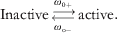
The conformational switch, referred to as gating, is assumed to be uncoupled to the translational and rotational diffusion of the reactant molecules. Again using the constant-flux approximation, Szabo et al. were able to express the ‘gated’ association rate constant, k G, to the Laplace transform of the ‘ungated’ rate coefficient:
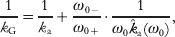
where ω0=ω0++ω0−. This result has been extended to the time-dependent rate coefficient k G(t) (in Laplace space) and to the case where both reactant molecules are gated (Zhou & Szabo, Reference Zhou and Szabo1996a).
When the gating is slow (i.e., ω0+ and ω0−→0), ω0a(ω0)→k a; Eq. (4.49) becomes
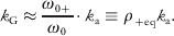
In this limit, a ligand molecule can contribute to the inward flux on the inner boundary only if it is initially in the active conformation, which it adopts with the equilibrium probability ρ+eq. Hence, the total rate constant is this equilibrium probability times the rate constant for a ligand molecule that stays in the active form. In the opposite limit (i.e., ω0+ and ω0−→∞), ω0a(ω0)→k a(0); therefore,
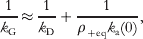
where we have expressed k a in terms of k D and k a(0) [see Eq. (4.32a)]. This is the rate constant for ungated binding with effective reactivity ρ+eqκ; that effective reactivity is just what is expected when the conformational switch is fast. If the binding of the active form is diffusion controlled, i.e., κ→∞, Eq. (4.50b) reduces to k G≈k D. That is, the diffusion-controlled rate constant is unhindered when the conformational switch is fast. This result is very significant. It means that diffusion-controlled rate constants calculated under the assumption that the reactant molecules are frozen in their native conformations, as is the case for the transient-complex theory, are valid as long as the conformational fluctuations of the reactant molecules are fast.
The calculation of k G(t), based on a single protein–ligand pair, is the same whether the protein or ligand is gated. However, the solution to the many-body problem of a protein molecule surrounded by an excess of ligand molecules does depend on which reactant is gated (Zhou & Szabo, Reference Zhou and Szabo1996b). When the ligand molecules are gated, effectively they independently bind with the protein molecule, and Eq. (4.17b) still holds for the survival probability of the protein, except that the rate coefficient is now replaced by k G(t):
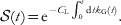
However, when the protein molecule is gated, the dynamics of the ligand molecules around it become coupled: when the protein undergoes an active to inactive switch, all the surrounding ligand molecules simultaneously sense a change in the boundary condition from radiation to reflection. Zhou & Szabo (Reference Zhou and Szabo1996b) proposed the following rate equations:

for the probabilities,  c(t), that the protein survives at time t while in conformation c, c=‘a’ for active and ‘i’ for inactive, respectively; (t)=a(t)+i(t). The solution of these rate equations is in good agreement with computer simulations. Under fast gating, Eq. (4.51b) reduces to Eq. (4.51a).
Some enzymes have buried active sites, with narrow tunnels leading to the exterior; conformational fluctuations of bottlenecks, or gates, along the tunnels must occur to allow for substrate access and product release (Zhou & McCammon, Reference Zhou and Mccammon2010). When a gate along the tunnel to the active site switched between closed and open states according to scheme (4.48), an approximate result for the gated binding rate constant similar to Eq. (4.49) was found (Zhou, Reference Zhou1998):
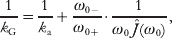
where k a again is the ungated rate constant and J(t) is the total flux across the gate at time t when the substrate was started from an equilibrium distribution confined to the outside of the gate. Ĵ(s) has the following limiting values:


where A g is the area of the gate and 〈· · ·〉g denotes an average over the cross-section of the gate. Using these results, we can find the gated rate constant in the slow gating limit:

and in the fast gating limit:

The last result states that, under fast gating, the gated rate constant approaches the ungated rate constant, even if binding when the gate is open is not limited by diffusion.
Zhou et al. (Reference Zhou, Wlodek and Mccammon1998b) used Eq. (4.52) to study the substrate binding rate constant to acetylcholinesterase, an enzyme with a buried active site but still affording one of the highest k cat/K M values, at ~109 M−1 s−1 (Nolte et al. Reference Nolte, Rosenberry and Neumann1980; Ordentlich et al. Reference Ordentlich, Barak, Kronman, Flashner, Leitner, Segall, Ariel, Cohen, Velan and Shafferman1993; Pryor et al. Reference Pryor, Selwood, Leu, Andracki, Lee, Rao, Rosenberry, Doctor, Silman and Quinn1992; Vellom et al. Reference Vellom, Radic, Li, Pickering, Camp and Taylor1993). Analysis of the gating dynamics obtained from molecular dynamics simulations showed that, for the intended substrate, acetylcholine, it is close to the fast-gating regime, and the gated rate constant is lower than the ungated rate constant by just 2-fold, even though ρ+eq is only 2%. Combined with the ungated rate constant previously calculated from Brownian dynamics simulations (Zhou et al. Reference Zhou, Briggs and Mccammon1996), the gated rate constant is found to be in the range of measured k cat/K M values. However, for a somewhat larger substrate, modeling butyrylcholine, the gated rate constant is three orders of magnitude lower (ρ+eq decreases to 8×10⁻⁵), in line with similar decreases in k cat/K M observed for that substrate (Ordentlich et al. Reference Ordentlich, Barak, Kronman, Flashner, Leitner, Segall, Ariel, Cohen, Velan and Shafferman1993; Pryor et al. Reference Pryor, Selwood, Leu, Andracki, Lee, Rao, Rosenberry, Doctor, Silman and Quinn1992; Vellom et al. Reference Vellom, Radic, Li, Pickering, Camp and Taylor1993). Conformational gating thus affords the enzyme exquisite substrate selectivity. That gating is essential in the selectivity is supported by the observation that when bulky side chains constituting the gate are mutated into smaller ones, presumably bringing the gating dynamics for butyrylcholine toward the fast-gating regime through an increase in ρ+eq, k cat/K M for butyrylcholine is significantly increased (Ordentlich et al. Reference Ordentlich, Barak, Kronman, Flashner, Leitner, Segall, Ariel, Cohen, Velan and Shafferman1993; Pryor et al. Reference Pryor, Selwood, Leu, Andracki, Lee, Rao, Rosenberry, Doctor, Silman and Quinn1992; Vellom et al. Reference Vellom, Radic, Li, Pickering, Camp and Taylor1993).
4.5 Intermolecular versus intramolecular binding
When the protein and ligand are covalently linked, their binding becomes intramolecular. Under an approximate treatment of the linker, a simple relation between the equilibrium constants of the inter- and intramolecular binding processes has been derived (Zhou, Reference Zhou2001b; Zhou & Gilson, Reference Zhou and Gilson2009). The linker is assumed to be flexible and to have negligible interactions with the protein and the ligand; the end-to-end distance at which the probability density, ρL(r), of the end-to-end vector r is maximal is assumed to be much greater other relevant lengths, such as the size of the native-complex energy well, and the range of a long-range potential if present. Then

Throughout this subsection we use a superscript L to denote quantities for the intramolecular process; a denotes the end-to-end vector in the native complex. What are the corresponding relations between the rate constants of the inter- and intramolecular binding processes?
When the binding is activation controlled, it is easy to see that


When the binding is diffusion controlled, these relations for the rate constants still hold if K aL=K aρL(a)≪1 and the linker does not affect the relative diffusion constant of the protein and ligand. The justification is the same as the one leading to Eq. (4.46), which captures the effect of long-range electrostatic attraction on k a (Zhou, Reference Zhou2002, Reference Zhou2001c). A check of Eq. (4.56a) is provided by the rate constant for the diffusion-controlled end-to-end contact formation of a polymer chain obeying Gaussian statistics, obtained by Szabo et al. (Reference Szabo, Schulten and Schulten1980) by calculating the mean first passage time. Let the contact distance be a and the mean square of the end-to-end distance be 〈r 2〉. The probability density for the end-to-end vector is (3/2π〈r 2〉)3/2exp(−3r 2/2〈r 2〉). When a≪〈r 2〉1/2, which is equivalent to K aL≪1, Szabo et al.'s result is

The first factor, 4πDa, can be recognized as the diffusion-controlled rate constant for intermolecular contact formation; the second factor, (3/2π〈r 2〉)3/2, can be recognized as the probability density of the end-to-end vector at r=a [when a≪〈r 2〉1/2, exp(−3a 2/2〈r 2〉)→1]. Hence, Szabo et al.'s result conforms to Eq. (4.56a).
Equation (4.55) has been used to derive the association constant for a bivalent ligand, which features two fragments connected by a linker; the framents bind to two separate sites (named 1 and 2) on the protein (Zhou, Reference Zhou2001b). After binding the first fragment, the binding of the second fragment becomes intramolecular. The overall association constant of the bivalent ligand is thus

Here we use a superscript B to denote quantities for the bivalent ligand; K a1 and K a2 are the association constant for the first fragment when the second is absent and vice versa; and a again denotes the end-to-end vector of the linker in the native complex.
The native complex can be formed by first occupying site 1 and then site 2 or by proceeding in the reverse order:
Making a steady-state approximation for each singly bound species, the overall rate constant for binding the bivalent ligand is
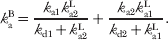
Applying the approximation of Eq. (4.56a) to k a1L and k a2L and expressing k d1 and k d2 as k a1/K a1 and k a2/K a2, respectively, we find (Zhou, Reference Zhou2003b)

However, validity of Eq. (4.56a) requires that K a1ρ(a) and K a2ρ(a)≪1; hence,

4.6 Reversibility
Up to now we have treated the protein–ligand binding process as though it is irreversible. The kinetics of reversible diffusion-influenced binding has long attracted the attention of theorists (Agmon, Reference Agmon1984; Gopich & Doktorov, Reference Gopich and Doktorov1996; Gopich & Szabo, Reference Gopich and Szabo2002; Lee & Karplus, Reference Lee and Karplus1987; Lukzen et al. Reference Lukzen, Doktorov and Burshtein1986; Naumann, Reference Naumann1994; Szabo, Reference Szabo1991; Yang et al. Reference Yang, Lee and Shin1998). For simplicity we only consider the pseudo-first-order limit, where effectively a single protein molecule is surrounded by excess ligand molecules. Upon binding with one ligand molecule, the protein surface becomes reflecting for all the other diffusing ligand molecules. The fact that the binding of a single ligand molecule instantaneously changes the boundary condition for the diffusion of all the other ligand molecules renders the problem many-body in nature. In general the kinetics is quite complicated, but under two limiting situations it is simplified. The first is when diffusion is infinitely fast (and the binding is thus activation controlled). Then a newly released ligand molecule will immediately equilibrate with the other ligand molecules to reach the equilibrium distribution, and consequently the ordinary rate equation, Eq. (2.15), applies. The relaxation function Y(t)=[C P(t)−C Peq]/[C P(0)−C Peq] is then given by Eq. (2.16), with the association rate constant k a replaced by the activation-controlled limit k A. In Laplace space, the relaxation function is
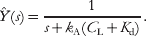
The second limiting situation is when binding and unbinding are under the influence of diffusion but occur infrequently. Then a newly released ligand molecule will have sufficient time, before the next binding event, to equilibrate with the other ligand molecules and reach the steady-state distribution of irreversible binding. Again, the ordinary rate equation applies for the relaxation of the protein concentration at times longer than that for reaching the steady-state distribution of irreversible binding, but now the association rate constant is the k a calculated in the preceding subsections under the assumption of irreversible binding.
When binding and unbinding are under the influence of diffusion and not infrequent, a newly released ligand molecule and the other ligand molecules do not have sufficient time to relax to the steady-state distribution of irreversible binding; the concentration of ligand molecules around the protein will thus be somewhat higher than expected from that distribution, and hence the effective binding rate constant will be higher than the k a for irreversible binding.
Gopich & Szabo (Reference Gopich and Szabo2002) devised a self-consistent relaxation time approximation for the kinetics of reversible diffusion-influenced binding. In Laplace space, their relaxation function is given by
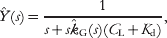
where

has a structure similar to a gated rate coefficient for irreversible binding [see Eq. (4.49)]. The ‘gating’ rate k 0 is determined self-consistently by requiring that the area under the relaxation function, i.e., Ŷ(0), is the inverse of k 0. When diffusion is infinitely fast, s a(s) and s G(s)→k A and Eq. (4.60a) reduces to Eq. (4.59). The connection to a gated rate coefficient for irreversible binding comes from the fact that the unbound protein allows the surrounding ligand molecules to bind but the bound protein is reflecting to them. Notice, however, that Eq. (4.60b) differs from Eq. (4.49) by the appearance of ρbeq on the left-hand side. As a result, here s G(s)>s a(s), an outcome already anticipated in the preceding paragraph. In contrast, gating transition from an active form to an inactive from always reduces the rate coefficient for irreversible binding.
5. Macromolecular crowding
In applying rate theories to model cellular functions, one must account for the effects of the crowded environments inside cells. Macromolecular crowding is expected to significantly affect kinetic properties of proteins and nucleic acids (Zhou et al. Reference Zhou, Rivas and Minton2008). In general, macromolecular crowding can be treated implicitly by accounting for its effects on the energy functions and dynamics of the reactant molecules (Minton, Reference Minton, Srere, Jones and Mathews1989; Zhou, Reference Zhou2004).
In a 1991 paper (Zhou & Szabo, Reference Zhou and Szabo1991), the implicit treatment of macromolecular crowding was directly tested against molecular dynamics simulations. [These simulations (Dong et al. Reference Dong, Baros and Andre1989; Zhou & Szabo, Reference Zhou and Szabo1991) are probably the earliest on protein–protein association under crowded conditions; interest in such simulations has been revived (Kim & Yethiraj, Reference Kim and Yethiraj2009; Wieczorek & Zielenkiewicz, Reference Wieczorek and Zielenkiewicz2008).] The total simulation system consisted of a box of 500 hard spheres, occupying a total volume fraction of 41%. The hard spheres underwent ballistic motion and elastic collision. One of the hard spheres was labeled as protein P, different numbers of other hard spheres were labeled as protein L, and the remaining hard spheres as crowders. Whenever an L sphere collided with the P sphere, a complex was considered to be formed instantaneously. From the simulation trajectories, the survival probability of protein P at different times was obtained. The survival probability agreed well with the prediction of Eq. (4.17b), when the rate coefficient was calculated according to the centrosymmetric model of subsubsection 4.3.1 with a radiation boundary condition. The relative diffusion constant and the effective interaction potential of the associating proteins implicitly accounted for the effects of the crowders. This study demonstrates that rate theories can work under crowded conditions after the energetic and dynamic determinants of the rate constant are corrected for crowding effects. It is now possible to simulate the Brownian motions of concentrated protein molecules represented at a realistic level (McGuffee & Elcock, Reference Mcguffee and Elcock2006); such simulations will provide a new test ground for rate theories.
Below we present some theoretical results on how macromolecular crowding affects the dynamics and energetics of reactant molecules.
5.1 Effects on diffusion constants
It seems that not much attention has been paid by theorists to how internal dynamics of macromolecules is affected by crowding, although the problem has been studied by molecular dynamics simulations (Cheung et al. Reference Cheung, Klimov and Thirumalai2005; Minh et al. Reference Minh, Chang, Trylska, Tozzini and Mccammon2006; Mittal & Best, Reference Mittal and Best2010; Qin et al. Reference Qin, Minh, Mccammon and Zhou2010). On the other hand, the problem of how the translational diffusion constant of a macromolecule is affected by crowding is a classical problem. The theory of Tokuyama & Oppenheim (Reference Tokuyama and Oppenheim1994, Reference Tokuyama and Oppenheim1995), for a tracer hard sphere crowded by other identical hard spheres, is one of the most rigorous. Each particle undergoes Brownian motion, with diffusion constant D, were it not for hydrodynamic interactions and collisions with other particles. The effective diffusion constant of the tracer particle, as a function of the crowder volume fraction Φ, is given by
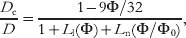
where

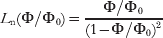
with b 1=(9Φ/8)1/2, b 2=11Φ/6, and Φ0≈0·5718. The numerator of the right-hand side of Eq. (5.1a) accounts for collisions, the L l(Φ) term accounts for local hydrodynamic interactions (arising from a static distribution of neighboring particles), and the L n(Φ) term accounts for non-local hydrodynamic interactions (arising from a relaxed distribution of neighboring particles). For a mixture of different-sized ‘soft’ crowders, Tokuyama (Reference Tokuyama2009a, Reference Tokuyamab) suggests fitting experimental data according to the following formula:

with η and Φ0 as adjustable parameters.
At Φ=0·3, which approximates the level of intracellular crowding (Zimmerman & Trach, Reference Zimmerman and Trach1991), Eq. (5.1a) predicts a 5-fold reduction in diffusion constant. This is generally consistent with the extent of crowding-induced reduction in translational diffusion constant measured on proteins in cytoplasm and concentrated solutions (Kuttner et al. Reference Kuttner, Kozer, Segal, Schreiber and Haran2005; Li et al. Reference Li, Wang and Pielak2009; Swaminathan et al. Reference Swaminathan, Hoang and Verkman1997). These experiments also show that rotational diffusion constants are reduced to a lesser extent, as to be expected. Similarly, one expects the effect of crowding on the effective friction coefficient or diffusion constant for internal dynamics to be relatively modest.
5.2 Effects on free energies of transition states and transient complexes
Crowding also affects the energy functions of macromolecules. A universal and significant aspect of the crowding effect, known as excluded-volume interactions, arises from the fact that molecules cannot occupy the same region in space. Excluded-volume interactions increase the free energy of a macromolecule, but the increase depends on its conformation. Compared to a more open conformation, a compact conformation is more easily accommodated into a distribution of crowders, and hence the crowding-induced increase in free energy, ΔG c, is less. Effectively, crowding changes the relative stability between these two conformations in favor of the latter. According to scaled particle theory (Lebowitz et al. Reference Lebowitz, Helfand and Praestgaard1965), ΔG c for a spherical test particle (with radius R p) crowded by other spherical crowders (with radius R c and occupying a volume fraction Φ) is
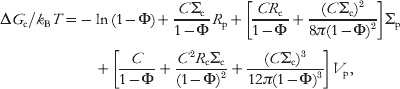
where C is the number density of the crowders, Σc and Σp are the surface areas of the crowders and the test particle, respectively, and V p is the volume of the test particle. As to be expected, ΔG c increases with increasing R p. A recent development extends Eq. (5.3) to atomistic proteins, with the geometric parameters R p, Σp, and V p calculated from protein conformations (Qin and Zhou, Reference Qin and Zhou2010).
When a protein undergoes a folding transition, the transition state is more compact than the unfolded state. Excluded-volume interactions with crowders are thus expected to stabilize the folding transition state. If it is assumed that the effective diffusion constant along the folding reaction coordinate is not affected (see preceding subsection), then crowding would increase the folding rate.
Similarly, crowding is expected to stabilize the transient complex of a protein–protein pair relative to the unbound state. Crowding thus produces two opposing contributions to the diffusion-controlled association rate constant: a decrease due to the reduction in translational (and to a less extent rotational) diffusion constant and an increase due to the stabilization of the transient complex. The two opposing contributions lead to a rather modest net effect by crowding. Assuming that the crowding-induced change in free energy, ΔΔG c, with the unbound state as a reference, is long ranged, one may adapt Eq. (4.46) to obtain the following result for the association rate constant under crowding (Zhou, Reference Zhou2004):

where k a is the rate constant in a dilute solution and <ΔΔG c>* is the average of ΔΔG c in the transient complex. [An additional factor, arising from the disparate effects of crowding on translational and rotational diffusion constants, may also be introduced; see Eq. (4.36d).] Calculations suggest that ΔΔG c, like electrostatic attraction between two proteins, is indeed long ranged (Qin, Lu, and Zhou, to be published).
6. Illustrative applications
We now present several examples to illustrate how rate theories can be used to yield insight at the microscopic level on proteins and DNA undergoing transitions.
6.1 Unfolding/unzipping under force
The unfolding of proteins, unzipping of nucleic acids, and dissociation of protein–ligand complexes have been studied in many single-molecule ‘pulling’ experiments (Cao et al. Reference Cao, Kuske and Li2008; Carrion-Vazquez et al. Reference Carrion-Vazquez, Oberhauser, Fowler, Marszalek, Broedel, Clarke and Fernandez1999; Chen et al. Reference Chen, Wen and Tinoco2007; Greenleaf et al. Reference Greenleaf, Frieda, Foster, Woodside and Block2008; Kellermayer et al. Reference Kellermayer, Smith, Granzier and Bustamante1997; Liphardt et al. Reference Liphardt, Onoa, Smith, Tinoco and Bustamante2001; Marshall et al. Reference Marshall, Sarangapani, Lou, Mcever and Zhu2005; Mathé et al. Reference Mathé, Visram, Viasnoff, Rabin and Meller2004; Merkel et al. Reference Merkel, Nassoy, Leung, Ritchie and Evans1999; Rief et al. Reference Rief, Gautel, Oesterhelt, Fernandez and Gaub1997, Reference Rief, Clausen-Schaumann and Gaub1999; Schlierf & Rief, Reference Schlierf and Rief2006; Yang et al. Reference Yang, Cecconi, Baase, Vetter, Breyer, Haack, Matthews, Dahlquist and Bustamante2000). As the pulling force is increased monotonically with time, at some point the system undergoes an unfolding/unzipping (or dissociation) transition. The pulling force at that point is referred to as the rupture force. The transition can be modeled as a rate process, with the rate coefficient k u affected by the time-dependent pulling force F(t). The survival probability of the intact system is then governed by (Evans & Ritchie, Reference Evans and Ritchie1997)

which has the solution

For a stiff system pulled at a constant speed v by a spring with spring constant κs, one has F=κsvt and  =κsv. The probability density of the rupture force, ρ(F), is related to the survival probability via

Hence,
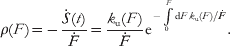
If k u(F) is calculated from a theory (see below), Eq. (6.2b) can be used to predict the distribution of the rupture force.
Experimentalists face the reverse problem: they measure the distribution of the rupture force and want to extract k u(F) from their data.Footnote 5 To that end, one rearranges Eq. (6.1a) to express k u(F) in terms of S(t) and its time derivative and then uses Eq. (6.2a) to express the latter two quantities in terms of ρ(F). The result is
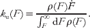
As observed by Dudko et al. (Reference Dudko, Hummer and Szabo2006, Reference Dudko, Hummer and Szabo2008), data collected at different pulling speeds and analyzed according to Eq. (6.3) should all collapse to the same curve.
Now we consider the calculation of k u(F). The unfolding/unzipping transition can be modeled as an escape from a potential well along the pulling direction. The pulling force modifies the potential function from U 0(x) to U 0(x)−Fx, where x is the coordinate along the pulling direction. Assuming that the motion along x is diffusive, Kramers' formula [Eq. (3.44)] predicts the force-dependent rate coefficient as (Evans & Ritchie, Reference Evans and Ritchie1997; Shapiro & Qian, Reference Shapiro and Qian1997)

where k u0 is the rate coefficient in the absence of force, and well and barrier mean that the integrations are restricted to these regions. Dudko et al. (Reference Dudko, Hummer and Szabo2006) evaluated these integrals approximately for a quadratic-cusp form and a linear-cubic form of U 0(x). The results in both cases can be written as

where ν=1/2 and 2/3 for the two forms of potentials, respectively; ΔU‡ is the activation energy of U 0(x); and Δx‡ is the displacement between the bottom of the well and the top of the barrier. When ν=1, Eq. (6.5) reduces to Bell's formula (Bell, Reference Bell1978).
Dudko et al. (Reference Dudko, Hummer and Szabo2008) analyzed data from two single-molecule experiments. One studied the unfolding of a protein by atomic force microscopy (Schlierf & Rief, Reference Schlierf and Rief2006); the other studied the voltage-induced unzipping of a DNA pair in a nanopore (Mathé et al. Reference Mathé, Visram, Viasnoff, Rabin and Meller2004). The data from each experiment, collected at different pulling or voltage-ramp speeds, when processed according to Eq. (6.3), collapsed to a single curve, yielding k u(F). They then fitted these k u(F) to Eq. (6.5) to generate values for the microscopic parameters k u0, ΔU‡, and Δx‡.
6.2 Kinetics of fluctuating enzymes
Single-molecule experiments have revealed that a single enzyme can produce a wide range of turnover rates, presumably due to conformational fluctuations (Antikainen et al. Reference Antikainen, Smiley, Benkovic and Hammes2005; English et al. Reference English, Min, Van Oijen, Lee, Luo, Sun, Cherayil, Kou and Xie2006; Flomenbom et al. Reference Flomenbom, Velonia, Loos, Masuo, Cotlet, Engelborghs, Hofkens, Rowan, Nolte, Van Der Auweraer, De Schryver and Klafter2005; Lu et al. Reference Lu, Xun and Xie1998; Shi et al. Reference Shi, Dertouzos, Gafni, Steel and Palfey2006; van Oijen et al. Reference Van't Hoff2003; Zhang et al. Reference Zhang, Rajagopalan, Selzer, Benkovic and Hammes2004). In particular, English et al. (Reference English, Min, Van Oijen, Lee, Luo, Sun, Cherayil, Kou and Xie2006) followed events of turning over a fluorogenic substrate by β-galactosidase. The turnover rates at each substrate concentration fluctuate widely, but the dependence of the average rate, as measured by the inverse of the average waiting time, 〈τ〉, between turnover events, on substrate concentration conforms to the Michaelis–Menten relation. This apparent Michaelis–Menten behavior initially was explained by invoking the assumption that conformational exchanges in the enzyme–substrate complex are extremely slow (i.e., in the quasi-static limit) (Kou et al. Reference Kou, Cherayil, Min, English and Xie2005). A later reexamination suggested that the Michaelis–Menten behavior was the result of a very small k cat (i.e., satisfying the quasi-equilibrium condition) (Min et al. Reference Min, Gopich, English, Kou, Xie and Szabo2006; see also Qian, Reference Qian2008).
The sequence of waiting times contains rich information. Besides the average, the distribution function φ(τ) and the correlation function ci=〈(τi−〈τ〉)(τ0−〈τ〉)〉, where τi is the ith waiting time, are useful. Min & Xie (Reference Min and Xie2006) showed that the correlation function measured on β-galactosidase (English et al. Reference English, Min, Van Oijen, Lee, Luo, Sun, Cherayil, Kou and Xie2006) is mimicked by the correlation between events of crossing a tiny (0·1 k BT) energy barrier in a double-well potential, when the dynamics is governed by the generalized Langevin equation with a power-law memory kernel. That memory kernel itself was motivated by the observed dynamic behavior of the distance between the electron donor and acceptor in a protein (Min et al. Reference Min, Luo, Cherayil, Kou and Xie2005). The fluctuations of the distance were modeled well as a particle moving in a harmonic well according to the generalized Langevin equation with a power-law memory kernel.
6.3 Protein folding and association under crowding
Ai et al. (Reference Ai, Zhou, Bai and Choy2006) measured the folding and unfolding rate constants of a four-helix bundle protein under crowding. In the presence of 85 g l−1 of a crowding agent, PEG 20 K, the folding rate constant is increased by 2-fold but the unfolding rate constant is essentially unchanged. Qualitatively, these observations are consistent with crowding effects dominated by excluded-volume interactions. To carry out a quantitative test, the transition-state ensemble of this protein was generated from molecular dynamics simulations (Tjong & Zhou, Reference Tjong and Zhou2010). It consists of highly compact conformations with residual secondary structures. Calculations of crowding effects on the transition-state ensemble yield changes in folding and unfolding rate constants that are in agreement with experimental results.
Yuan et al. (Reference Yuan, Chyan, Zhou, Chung, Peng, Ping and Yang2008) studied the effects of crowding on the pulling force required to unfold ubiquitin. Compared to the result in a dilute solution (unfolding force at 210 pN), the unfolding force increases by 24 pN when the concentration of a crowding agent, dextran 40 K, is increased to 300 g l−1. The increase in pulling force was interpreted as the reflection of a decrease in the unfolding rate constant. The latter in turn was attributed to the destabilization of the transition state, relative to the more compact folded state, by dextran crowding. By representing the transition state as a sphere somewhat enlarged from the folded state and using Eq. (5.3) to calculate the change in activation energy by crowding, the experimental results could be explained.
Kuttner et al. (Reference Kuttner, Kozer, Segal, Schreiber and Haran2005) studied how PEG 8 K affects the association rate constant of two proteins. To dissect the contributions of crowding, they also measured the effects of the crowding agent on translational and rotational diffusion constants of proteins. As already noted in subsection 5.1, crowding affects the two types of diffusion constants to different extents. After correcting for the reductions in diffusion constants, Kuttner et al. found that the association constant is higher than expected, implicating a crowding-induced stabilization of the transient complex; the stabilization is ~0·8 k BT, in line with calculations (Qin, Lu, and Zhou, to be published).
7. Conclusion and outlook
We have summarized some of the rate theories that are most useful for modeling biological processes. Highlighted are strengths and limitations of different theories and their interconnections, in particular between those for unimolecular reactions and those for bimolecular reactions. Examples are presented to demonstrate that rate theories can help generate insight at the microscopic level into biomolecular behaviors.
In general, rate constants depend on both the energetics and the dynamics of reaction coordinates. In developing rate theories, a minimum requirement is that the ratio of the forward and reverse rate constants is the same as the equilibrium constant, which only depends on energetics. If a theory, such as the transition-state theory, is based on classical statistical mechanics, then the final result for the rate constant should not include Planck's constant, which is a signature of quantum effects.
The Smoluchowski model of diffusion-controlled non-specific binding between spherical particles is inappropriate for stereospecific protein–ligand binding. Rather, because of the orientational constraints arising from the stereospecificity, the limit of the rate constant set by random diffusion is several orders of magnitude lower than the Smoluchowski result. Two mechanisms have been proven to provide rate enhancement: long-range attraction provided by protein–ligand electrostatic interactions and reduction of dimensionality provided by non-specific binding.
Active developments can be anticipated in several areas:
1. Implementation of rate theories through computer simulations. While in principle it is possible to simulate the motions of reactant molecules as a whole and observe rare transitions between states, it is far more practical and perhaps more insightful to focus on a small number of coordinates that are intimately related to these transitions. The problem then becomes one of calculating potentials of mean force and effective friction coefficients or diffusion constants for these coordinates. The prospect of combining these modeling efforts with experimental probes is particularly exciting.
2. Application of rate theories to complex biological processes involving multiple steps. Examples of such processes include chaperonin-assisted protein folding and translation of mRNA into protein (Martin et al. Reference Martin, Mayhew, Langer and Hartl1993; Rodnina et al. Reference Rodnina, Gromadski, Kothe and Wieden2005). Mechanistic models of such processes often assume an ordered sequence of steps. In reality, side reactions (such as binding of non-cognate aminoacyl-tRNAs to the decoding center) occur alongside on-pathway reactions. In the same way that reaction coordinates capture the essence of inter-state transitions, it can be anticipated that dominant pathways emerge in the midst of all possible side reactions, thus providing a theoretical basis for an ordered-sequence description.
3. Application of rate-theory techniques to the modeling of other biological problems. In particular, the transport of ions across transmembrane protein channels (Berezhkovskii & Bezrukov, Reference Berezhkovskii and Bezrukov2004; Berneche & Roux, Reference Berneche and Roux2003; Goychuk & Hanggi, Reference Goychuk and Hanggi2002; Lear, Reference Lear2003; Lauger et al. Reference Lauger, Stephan and Frehland1980; Levitt, Reference Levitt1986; Roux et al. Reference Roux, Allen, Berneche and Im2004; Yi et al. Reference Yi, Cross and Zhou2009) and the generation of directed movement or rotation by motor proteins (Astumian, Reference Astumian1997; Bier, Reference Bier2003; Bustamante et al. Reference Bustamante, Keller and Oster2001; Gao et al. Reference Gao, Yang and Karplus2005; Junge, Reference Junge1999; Kinosita et al. Reference Kinosita, Adachi and Itoh2004; Kolomeisky & Fisher, Reference Kolomeisky and Fisher2007; Okada & Hirokawa, Reference Okada and Hirokawa2000; Qian, Reference Qian1997, Reference Qian2000; Wu et al. Reference Wu, Gao and Karplus2007; Xing et al. Reference Xing, Wang, Dimroth, Von Balmoos and Oster2004; Yildiz et al. Reference Yildiz, Tomishige, Vale and Selvin2004; Zhou & Chen, Reference Zhou and Chen1996) are amenable to mathematical models similar to those for chemical reactions (Zhou, Reference Zhou2005a). Cross-fertilization among different areas will accelerate theoretical development in each area and perhaps lead to a unifying theoretical framework.
4. More realistic modeling of crowding effects in calculations of rate constants. An atomistic model of crowders and inclusion of interactions in addition to the excluded-volume type will greatly increase the realism in representing intracellular environments. With such increased realism, theories will be able to produce rate constants that can be used in systems biology studies.
8. Acknowledgements
This paper was supported in part by Grant GM58187 from the National Institutes of Health. I thank J. Andrew McCammon, Olga Dudko, Hong Qian, and Cai Lu for reading the manuscript and Attila Szabo and Alexander Berezhkovskii for discussion.