Small fish–big issues: the effect of trade policy on the global shrimp market

PETER DEBAERE

doi:10.1017/S147474561000011X

Small fish–big issues: the effect of trade policy on the global shrimp market

Published online by Cambridge University Press: 08 April 2010

PETER DEBAERE

Show author details

PETER DEBAERE*: Affiliation:
Darden Business School, University of Virginia, CEPR
*: *Email: DebaereP@darden.virginia.edu

Article contents

Abstract
The shrimp market
Model
Data description
Specification and results
Conclusion
Footnotes
References

Rights & Permissions

Abstract

It is a well-established theoretical result that the trade policy of a large country can directly affect its own and other countries' welfares by affecting international goods' prices. However, there exist very few empirical studies that analyze the effect of trade policy on international prices. With detailed data on unit values and tariffs, I show how policy actions in Europe disrupted the global shrimp market in a non-negligible way and set the stage for the anti-dumping case in the United States. The loss of Thailand's preferential trade status in Europe and the international differences in food-safety standards during the antibiotics crisis shifted especially Thai, Vietnamese, and Chinese shrimp exports away from Europe toward the United States in the late 1990s and early 2000s. I document how those shifting markets have decreased US prices for shrimp significantly compared to those in Europe.

Information

Type: Review Article
Information: World Trade Review , Volume 9 , Issue 2 , April 2010 , pp. 353 - 374

DOI: https://doi.org/10.1017/S147474561000011X [Opens in a new window]
Copyright: Copyright © Peter Debaere 2010

In 1997, the European Union retracted the preferential trade status of Thailand, the world's premier shrimp exporter. In 2001, antibiotics were found in shrimp residue, and the European Union (EU) declared a zero-tolerance policy that restricted exports especially from Vietnam and China. The EU also imposed 100% testing on shrimp from Thailand. Both events directly affected exporters' allocation decisions, away from Europe toward the United States. I use these two events to trace out the demand for shrimp in the United States versus Europe and to assess the impact of Europe's tariff and non-tariff policies on the price of shrimp in the United States versus Europe. My finding that the price of shrimp primarily responded to exogenous changes overseas is directly relevant for how one assesses the shrimp anti-dumping case in the US. At the same time, the analysis drives home a basic point that has so far found little empirical support: large countries through their trade policies can directly affect international prices. Finally, I show the non-negligible trade-diverting effects of international differences in food-safety standards, issues that will only become more important as talks about liberalizing agriculture proceed.Footnote ¹^, Footnote ²

In the fall of 2002, the Southern Shrimp Alliance from the US, a coalition of shrimp fishers, was formed to fight ‘unfair’ competition from developing countries. The Alliance called for punitive tariffs against Thailand, Vietnam, India, Brazil, Ecuador, and China. It charged US shrimpers were driven out of business by artificially low prices. Subsequently, the International Trade Commission ruled that the exporters injured the industry and the US Department of Commerce imposed high tariffs for Vietnam and China, and markedly lower ones for the others countries. The shrimp anti-dumping case emerged in an international shrimp market that had changed dramatically over the years. Increasingly, the global shrimp trade had become a one-way flow from developing-country producers to consumers in Europe, the United States, and Japan. To a large extent, aquaculture was responsible for the surge of shrimp production in developing countries. The shrimp that developed countries imported increasingly had been raised on farms in Asia and Latin America. This surge of imports in itself already posed a challenge for US shrimpers, who saw their US market share slip from 43% in 1980 to 12% in 2001 (Haby et al., Reference Haby, Miget, Falconer and Graham2002). Thailand's loss of its preferential tariff in Europe and the antibiotics crisis, however, increased this challenge even more and laid the groundwork for the anti-dumping case. As a matter of fact, my finding that tariff policy and antibiotics crisis increased the drop in the shrimp price reinforces the perception that anti-dumping policies are in many instances a modern form of protection to improve the competitive position of US shrimpers.

My findings also make a broader, more positive point. I use the events in the shrimp market as a natural experiment to investigate how large countries can affect international prices through their trade policies, a question that is difficult to analyze at the more aggregate level without getting caught in endogeneity issues.Footnote ³ The existing empirical literature on that subject, except for CGE models, is therefore limited and the small-country assumption that takes prices as given is mostly maintained. Exceptions are Romalis (Reference Romalis2005) and Chang and Winters (Reference Chang and Winters2002) in the context of preferential trade agreements.Footnote ⁴ Romalis (Reference Romalis2005) studies the impact of NAFTA on trade volumes and prices with disaggregate data. His results, like those of Chang and Winters (Reference Chang and Winters2002) for MERCOSUR, emphasize that especially price effects matter for countries' welfare, in spite of the substantial volume effects in trade liberalization studies.

My analysis strikes a balance between the view of, on the one hand, an integrated international market with only one world price and, on the other hand, that of partially localized markets. Romalis' (Reference Romalis2005) perfect competition setting is in the tradition of the first, whereas Chang and Winters (Reference Chang and Winters2002) relate better to the second approach with segmented markets.Footnote ⁵ Chang and Winters extend Feenstra (Reference Feenstra1989) who studies how tariffs are reflected in import prices. They introduce strategic interaction between exporters to one and the same foreign market. They find a significant effect of MERCOSUR on the pricing decisions of rivaling suppliers to Brazil. Like Chang and Winters (Reference Chang and Winters2002) and Feenstra (Reference Feenstra1989), I let exporters charge different prices in different markets, a fact well-documented by the pass-through literature that underscores that markets of internationally traded goods are localized.Footnote ⁶ However, I let prices in one market (United States) depend on the conditions in the other market (Europe) and vice versa. In particular, my exporter is constrained in his decision to allocate exports to various markets by a given amount of output − the shrimp harvest/catch.Footnote ⁷ This creates an explicit link between the localized market in the United States and in Europe. What the exporter sends to one market will not go to another. In this way, relocating exports from one country to another can change the relative prices in both markets and new policies in one market will affect the other.Footnote ⁸

I study shrimp exports for five of the countries subject to the anti-dumping case (Thailand, Vietnam, China, India, and Ecuador) plus Indonesia. These exporters had a significant and continuous presence in both the United States and European Union market between 1996 and 2004 and monthly data are available for that period.Footnote ⁹ Before discussing the model, data, and specification, I first sketch the context of the shrimp market.

1. The shrimp market

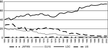
Estimates by the UN Food and Agriculture Organization [FAO] show a worldwide expansion of shrimp production from 0.31 million to 3.8 million metric tons between 1950 and 2002. A marked shift materialized in this period with a growing dichotomy between shrimp-consuming developed countries and shrimp-producing developing countries. As Figure 1 shows, the share of shrimp production by developing countries increased consistently and that of the main consumers – Japan, the United States, and Europe – steadily decreased. According to Haby et al. (Reference Haby, Miget, Falconer and Graham2002), Japan, Europe, and the United States currently consume some 60% of world production. International trade data tell a similar story. The FAO estimates consumption at 0.3 million metric tons of exports in 1976 and 1.7 million tons in 2002. The European Union, United States, and Japan together consistently absorb some 80% of these worldwide exports.

Figure 1.

Shares of world production (percentage)

Note: EU15 includes Austria, Belgium, Germany, Denmark, Spain, Finland, France, United Kingdom, Greece, Ireland, Italy, Luxembourg, Netherlands, Portugal, and Sweden; LDC comprises of Argentina, Brazil, Mainland China, Ecuador, Indonesia, India, Mexico, Malaysia, Philippines, Thailand, and Vietnam. All shares are relative to world shrimp production. The data cover some 70% to 90% of world shrimp production.Source: Calculations are based on FAO FishStat+. Total Production 1950–2002 database.

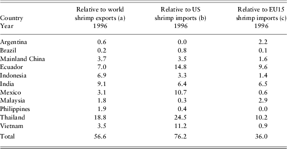
Table 1 lists the ten largest shrimp exporters into Europe and the United States for 1996, the beginning of our sample.Footnote ¹⁰ The list contains the six countries that we study: Thailand, China, Vietnam, Ecuador, Indonesia, and India. Throughout, as a fraction of total worldwide exports, Thailand is the most important exporter, and it plays a central role in our analysis. Together, the six countries account for about 70% of US imports in 1996. An important factor behind the sustained growth of shrimp supply is aquaculture. According to Haby et al. (Reference Haby, Miget, Falconer and Graham2002), it increases especially in the 1980s, starting from 5% of world production in 1980 to an impressive 30% at the end of the decade.Footnote ¹¹ In the 1990s, growth tapered off and aquaculture's share stabilized around 35%. Developing and emerging economies in general, and the countries that I study in particular, play a prominent role in shrimp farming. Shrimp farming requires waterfront property that in many developed countries has higher value in other uses. In addition, developing countries have a low-wage workforce, and they are also less restricted by environmental laws. Water pollution and the destruction of mangrove areas are sometimes linked to shrimp culture. Note finally that a country's shrimp output fluctuates significantly over time. Shrimp farming is risky. The crop is largely determined by weather and ecological conditions on the one hand. On the other hand, shrimp culture is also quite vulnerable to diseases that can severely reduce crops, as for China in 1993, Thailand in 1996 and 1997, and Ecuador in 1999.Footnote ¹²

Table 1.

Export quantity shares of some major shrimp producers in 1996 (percentage)

Sources:

(a) based on FAO FishStat+, Commodities production and trade 1976–2002 databases.

(b) Based on the NBER-managed trade database, Harmonized System Imports Commodity by Country, 1989–2001.

Traditionally, the United States had been a very open market for shrimp. Two events, however, disturbed this position:

Thailand's changing GSP status in the European Union

Until recently, the United States had no tariffs on shrimp imports. In Europe, however, the MFN tariff for frozen shrimp was 12% and that for cooked and canned shrimp 20%.Footnote ¹³ Since 1971, the European Union granted developing countries unilateral tariff reductions under the Generalized System of Preferences (GSP) to support industrialization.Footnote ¹⁴ In 1996 it was decided, to Thailand's surprise, to cut Thailand's GSP benefits for shrimp in half from January 1997 on and to abolish them by 1999. Under the European Union's GSP, raw and cooked shrimp were subject to respectively up to 4.5% and 6% tariff. From 1999 on, Thai shrimp faced an MFN tariff of 12% and 20%, while other exporters maintained their GSP status.

AntibioticsFootnote ¹⁵

In the summer and fall of 2001, reports surfaced in Europe about high levels of chloramphenicol and nitrofurans in shrimp shipments from East Asia. These antibiotics were banned in the European Union. While suspicion of widespread use of antibiotics in Asian shrimp farming gathered, there remained a significant difference between how the United States and the European Union addressed the antibiotics problem that contributed to the shift in the global shrimp market:

• The European Union had a zero-tolerance policy for chloramphenicol based on the minimum detectable limit. This limit declined with new technology and is between 0.1 parts and 0.3 parts per billion (ppb), much stricter than in the United States (initially 5 ppb).Footnote ¹⁶ The FDA gradually lowered its permissible limit to 1 ppb in May 2002 and to 0.3 ppb by the end of July 2003. Only when the crisis was virtually over in the fall of 2004 did the United States announce a testing method for nitrofurans and regular testing in 2005. The European Union limits nitrofurans to 1 ppbs.
• Enforcement also differed by destination. The European Union used temporary bans against Vietnam or China and subjected up to a 100% of Thai shipments to testing at the height of the crisis in 2002 and 2003, which caused costly delays of up to four weeks. Before the crisis, the European Union tested about 10% of Thai shrimp. Comparable measures for the United States are not available, but only in 2003 did the United States hire more inspectors to increase testing.
• To prevent contamination of the food chain, the European Union initially destroyed the affected imports. Only in September 2004, as the European Union was revising its zero-tolerance policy, did it consider the possibility of re-exporting or sending back to the exporter shrimp with lower ppbs.

The antibiotics crisis involved many shrimp exporters. Most seriously affected, however, were China, Vietnam, and Thailand. The crisis created according to seafoodbusiness.net quite some uncertainty for exporters. The European market for Asian shrimp, it states, had become a ‘crapshoot’ during this period. To ease the crisis, shrimp exporters explicitly banned the use of antibiotics. They imported measure kits to test goods before exporting and certified them. Transshipments (and re-labeling) of contaminated shrimps from other countries was restricted.Footnote ¹⁷ As with Thailand's loss of GSP status, food-safety concerns provided an unanticipated surge of shrimp exports to the United States, paving the way for the anti-dumping petition in December 2003.

2. Model

In this section, I present a simple model to guide the empirics. The model motivates the controls that are needed in order to assess the impact of tariff and non-tariff barriers on the price of shrimp. I focus on the decision of individual exporters to allocate exports between the European and US market. In a first step, I assume there are multiple exporters from different countries. While an exporter may in reality strategically reallocate some of his exports in response to what happens to other competitors, I assume that the exporter primarily responds to the restrictions in his own export market.

I assume that the demand for shrimp varieties and their substitutes, c, is determined at each moment in time by a CES utility function in the two destination markets, j, Europe and the United States. I suppress the time subscripts.

(1)

$U_{j} \equals \lsqb \rmSigma _{i} \lpar \gamma _{ij} c_{ij} ^{\lpar \sigma \minus \setnum{1}\rpar \sol \sigma } \rpar \rsqb ^{\sigma \sol \lpar \sigma \minus \setnum{1}\rpar } \quad \quad j \equals 1\comma 2$

where σ is the elasticity of substitution and typically larger than 1.

Optimization yields the familiar demand for good i in country j, c _ij.

(2)

$c_{ij} \equals \gamma _{ij} p_{ij} ^{ \minus \sigma } Y_{j}^{S}\sol P_{j}^{S\lpar\setnum{1} \minus \sigma\rpar } \quad \quad j \equals 1\comma 2$

P _j^S is a reference price index for shrimp varieties or more generally for other substitutes. It equals [Σ_i γ_ip _i^1−σ]^1/1−σ; p _ij is the actual price that consumers in country j pay for product i inclusive of tariffs; Y _j^s is the budget that country j spends on shrimp and comparable products.

I consider shrimp a product that is differentiated by country of origin and assume that there is complete international specialization in production. Therefore, c _ij coincides with j's total import demand for shrimp from country i. Since I am primarily interested in explaining shrimp prices and how these prices evolve over time, I rewrite equation (2) as follows:

(3)

$p_{ij} \equals \gamma _{ij} ^{\setnum{1}\sol \sigma } c_{ij} ^{ \minus \setnum{1}\sol \sigma } Y_{j}^{S\lpar\setnum{1}\sol \sigma \rpar } \sol P_{j}^{S\lpar \setnum{1} \minus \sigma \rpar \sol \sigma } \quad \quad j \equals 1\comma 2$

Equation (3) is an inverse demand function that states how much consumers are willing to pay for shrimp in country j. (I assume that p _i has a negligible impact on the aggregate price index.) Since I later argue that tariff changes only imply supply shifts, it is important to emphasize that the willingness to pay is expressed in terms of the actual price consumers pay. Therefore, there is no shift in demand (willingness to pay) when a tariff is imposed, as long as Y _j^s and P _j^S are not affected, which I assume. Note that prices are expressed in local currency since these are the relevant ones for consumers – consumers are no international arbitrageurs. To express euro prices in dollars, one simply multiplies the left and right side with the euro–dollar exchange rate.

I am especially interested in how the price of shrimp compares in the United States versus Europe. Equation (4) gives the equation that is the basis for my estimates and that is derived from equation (3). Following Chang and Winters (Reference Chang and Winters2002), I focus on real prices. Note that comparing shrimp prices in local currency as in equation (4) is identical to comparing their dollar prices – the exchange rate that is needed to convert euro prices into dollars on the left side will cancel since it is also needed to convert the right side into dollars.Footnote ¹⁸

(4)

$\ {{p_{i\setnum{1}} \sol P_{\setnum{1}} ^{S} } \over {p_{i\setnum{2}} \sol P_{\setnum{2}} ^{S} }}\ \equals \lpar \gamma _{i\setnum{1}} \sol \gamma _{i\setnum{2}} \rpar ^{\setnum{1}\sol \sigma } \lpar c_{i\setnum{1}} \sol c_{i\setnum{2}} \rpar ^{\minus \setnum{1}\sol \sigma } \ \left( {{{Y_{\setnum{1}} ^{S} \sol P_{\setnum{1}} ^{S} } \over {Y_{\setnum{2}} ^{S} \sol P_{\setnum{2}} ^{S} }}} \right)^{\setnum{1}\sol \sigma } \quad \quad j \equals 1\comma 2$

Equation (4) states that the relative consumption of the United States and Europe matters in these localized markets for how the relative shrimp price changes between those markets. Common movements underlying shrimp prices for countries 1 and 2 are differenced out. Moreover, as the analysis of relative supply x _i1/x _i2 that in equilibrium equals relative consumption c _i1/c _i2 will make clear, the localized prices are explicitly linked through the exporter's allocation decision, so that changes in one market affect the price in the other market. Let's now specify the supply side of the model.

In agricultural economics inverse demand systems that take the quantity as given are fairly common, especially in studies of local fish markets with high frequency data. An oft-cited study is Barten and Bettendorf (Reference Barten and Bettendorf1989). The motivation for this assumption is straightforward. Fish landings are fairly unpredictable because they are, to a large extent, determined by ecological circumstances and the weather. Moreover, since fish is perishable food, it has to be sold, so the amount that is caught determines the price.Footnote ¹⁹ While this logic is widely accepted, in an international context, there is an additional level of complexity. Even when the total harvest is in the short run exogenous, foreign suppliers still have to decide how much of their catch or harvest they send to one particular market. Consequently, how much shrimp exporters decide to export to the US versus the EU market does not only depend on the total harvest, it also depends on conditions in both markets.

Since the interconnectedness of international markets is key to the analysis and since I work with high-frequency data, I explicitly consider an exporter's short-term decision to allocate a given shrimp catch or harvest between two markets, which will be the United States and Europe.Footnote ²⁰ I assume that in order to maximize profits the exporter varies the export quantity between markets. In doing so, she can affect the price in different export markets. The exporter takes as given the tariffs and considers the price net of tariffs, the exchange rate, the marginal costs, and the conditions in the export markets. The exporter i maximizes the following profit function. I suppress the i subscripts for the different exporters.Footnote ²¹

(5)

$\eqalign{\tab \mathop {Max}\limits_{x_\setnum{1}\comma x_\setnum{2}} \ E_{\setnum{1}} \, \tilde{p}_{\setnum{1}} \lpar x_{\setnum{1}} \comma \bullet\! \rpar x_{\setnum{1}} \plus E_{\setnum{2}} \, \tilde{p}_{\setnum{2}} \, \lpar x_{\setnum{2}} \comma \bullet\! \rpar x_{\setnum{2}} \minus \alpha _{\setnum{1}} x_{\setnum{1}} \minus \alpha _{\setnum{2}} x_{\setnum{2}} \cr \tab {\rm s.t.}\quad X \equals x_{\setnum{1}} \plus x_{\setnum{2}} \comma \cr}$

where E _j refers to the exchange rate between country 1 or 2 and the exporter's home currency; x _j, refers to the quantity of the good exported to country j; $\tilde{p}_{j}$ is derived from equation (3) and is the price that the exporter receives, that is the price net of tariffs that is a function of e.a., x _j; α_j captures the marginal cost of exporting to market j, which among other things will be a function of bilateral distance.

I assume that the exporter maximizes profits in her domestic currency. She translates the foreign goods prices $\tilde{p}_{ij}$ into her own currency with the dollar and euro exchange rate. I assume that markets are localized, that is producers can charge a different price in different markets. I allow for different marginal costs α of delivering shrimp to one market versus to another. Needless to say that different α's could capture differences in transportation costs.Footnote ²² I assume that the exporter knows the conditions in her export markets, that is she knows relationships (3). She thus understands how quantities affect prices in both export markets and takes this into consideration as she decides on how much to send where. Moreover, the exporter's maximization is subject to the constraint that the exports to the United States and Europe add up to the exogenous quantity of the catch or harvest, X. Consequently, any amount that the exporter sends to the United States does not go to Europe and the reverse. In this way, in spite of the exporter's ability to charge a different price in different markets, the prices in Europe and the United States are closely linked. The exporter depresses the price in one localized market the more she exports to it, she props up the price in the other market where she exports less. The exporter's decision on how much to export to either market is a function of the characteristics of both markets, the exchange rates, and the marginal delivery costs. In this way, changes in the conditions of one market will affect the export supply to the other market.

(6)

$x_{ij} \equals f_{j} \lsqb \tau _{i\setnum{1}} \comma \tau _{i\setnum{2}} \comma Y_{\setnum{1}}^{S} \comma Y_{\setnum{2}}^{S} \comma P_{\setnum{1}}^{S} \comma P_{\setnum{2}}^{S} \comma E_{i\setnum{1}} \comma E_{i\setnum{2}} \comma X_{i} \comma \alpha _{i\setnum{1}} \comma \alpha _{i\setnum{2}} \rsqb \comma \quad \quad j \equals 1\comma 2$

where τ_i1 and τ_i2 refer to the tariffs in markets 1 and 2.

There is an important difference between my setup and that of Chang and Winters (Reference Chang and Winters2002), and Feenstra (Reference Feenstra1989) who consider a pricing decision (with market-specific marginal costs) that isolates markets from each other. I also allow for different prices across countries, yet I explicitly connect the different markets through the exporter's allocation decision (of a given harvest). Because of this decision, circumstances in Europe, such as the antibiotics crisis will affect the amount of shrimp sent to the United States. The central empirical question is then: to what extent does the exporter affect the relative price of shrimp as she shifts markets. Note that there are different ways to rationalize the antibiotics crisis in my setup. One possibility is to consider it a change in Europe's α; another option, since for China and Vietnam the crisis involves restrictions on the volume of exports, is to consider it really a constraint on how much x can go to Europe.Footnote ²³ In the latter case, if x were binding, the exporter would be unable to allocate his optimal choice of x to Europe and would be forced to export more to the United States than he wanted. There are also various ways in which my setup could be modified or generalized. One could wonder what would happen if instead of the exporter considered here, there were a multitude of small exporters from each country with no individual impact on the price in either market. If individual exporters took the behavior of other exporters as given, their allocation decision in response to tariff changes or an antibiotics crisis would ignore the joint impact of their reallocation away from Europe to the United States on the prices. They, therefore, might relocate more than in the case considered here, triggering more of a relative price adjustment. Note that such modifications of the setup would not alter the basic insight: the exporter's allocation decision links geographically separate markets, and it gives way to the question as to how relative prices move as she relocates exports in response to changing circumstances.

3. Data description

To estimate the model, I use monthly data between January 1996 and July 2004. My analysis hinges on a comparison of the United States and the European market. I therefore only include countries that have an uninterrupted time series of shrimp data in either market. I use public information on the volume and the value of shrimp imports (which does not include tariff, freight, insurance fees, and other surcharges) as well as on tariffs.

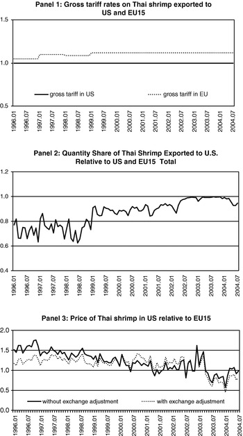
I retrieve tariff data for the US from the HTS archives of the USITC Web site and the TARIC database of the European Community. I focus on the HTS category 030613. This category excludes all the more-processed shrimp and prawn products, which is to say those that have been canned, frozen, and put into airtight containers or prepared with other fish or meat. These last products are categorized under the HTS category 160520. The six countries that we study faced a zero tariff in the US throughout the period. Note that the preliminary tariffs imposed by the US Commerce Department in the context of the anti-dumping case were announced only at the very end of the period that I study. For Europe, the specific tariff rates indicate that Vietnam, China, India, and Indonesia faced a tariff between 4.2% and 4.5% tariff for HTS 030613 before 1999. After 1999, the tariff was 4.2%. The only country with a consistently lower tariff is Ecuador with 3.6%, except for 1996 when it was 4.5%. In the wake of European Union's revision of its GPS tariff system, Thailand saw its initial 4.5% tariff increase. From 1997 onward, it faced a tariff of up to 9%. By 1999, Thailand had graduated from the GSP system and has faced the regular MFN tariff of 12% since then. In the analysis, I will focus on the tariff change in Thailand, since this is the only significant tariff variation there is in the data. The first panel of Figure 1 plots the gross tariff rate for Thai shrimp, 1+the ad valorem tariff rate in Europe. One clearly sees a stepwise increase in the tariff from 4.5% before the revision of Thailand's GSP status in 1997 to 9% and finally to 12% for frozen shrimp at the beginning of 1999 when Thailand gained full MFN status.

To compute the price of shrimp (unit value), I divide the value by the quantity. Shrimp imports for the United States are retrieved from the International Trade Commission's Web site, which provides US import from all the countries in the world. The imports are classified by Harmonized Tariff Schedule number and available at the ten-digit level. The values are reported in dollars, while the quantities are measured in pounds. Shrimp imports for Europe are provided by Europe's statistical agency, EUROSTAT. In our definition, Europe comprises 15 countries: Austria, Belgium, Germany, Denmark, Spain, Finland, France, United Kingdom, Greece, Ireland, Italy, Luxembourg, Netherlands, Portugal, and Sweden. The European import data are available at the eight-digit HTS level. The values are reported in euros, while the quantities are measured in kilogram. Only data on shrimp imports from the major exporters are available. I aggregate the data up to the six-digit HTS number to get a sizable group of countries that export both to the United States and Europe and to obtain exports that are comparable between the United States and Europe.Footnote ²⁴ Thailand, Vietnam, China, Ecuador, India, and Indonesia all have continuous time series in both Europe and the United States during the entire period.Footnote ²⁵

The second panel of Figure 2 plots data for Thai shrimp exports to the United States as a fraction of total exports to the United States and Europe and is very suggestive in illustrating how the Thai export market shifts away from Europe toward the United States. From initially 72% in 1996, the United States share increased to 89% in 1999 after the tariff hikes. Finally, the share rose even more with the antibiotics crisis in late 2001. By early 2004, it had reached 97%. The lowest panel of Figure 2 also shows a drop in the price of shrimp in the US vs Europe. Note that one observes similar shifts away from Europe to the United States for China and Vietnam around the antibiotics crisis, and corresponding movements in relative prices. The import shares and relative prices for the remaining countries that we study, however, did not change systematically around that time.Footnote ²⁶

Figure 2.

The shrimp market, prices, and export shares, 1996–2004

Source: USITC, EUROSTAT.

To proxy for aggregate prices, I retrieve the CPI and the food price index for the United States and Europe from the Main Economic Indicators database of the OECD's on-line library. As an imperfect proxy for real income, I retrieve the monthly (not cyclically adjusted) industrial production index from the Federal Reserve for the United States and from EUROSTAT for the same 15 countries of the European Union considered before. All of these indices have 2000 as the base year. The euro–dollar exchange rate is also taken from EUROSTAT. The exchange rate is a monthly average. To construct the aggregate shrimp price indices for Europe's and the US's main exporters, I use the unit values from the aggregate exports to the United States and European Union from their 11 most important exporters, respectively for HTS 030613 and 160520 combined (‘ShrimpII’) and HTS 030613 (‘ShrimpI’).Footnote ²⁷

The antibiotics crisis started in the summer of 2001 when high levels of antibiotics were discovered in shrimp residue. I take this as the starting point for a dummy that should capture the effect of the antibiotics crisis. While a dummy measure is a crude proxy, there is, however, no other measure available to capture the intensity of the crisis. By the fall of 2004, at the end of the data set, the crisis is largely over. Testing intensities have been reduced, and the restrictions reduced and abolished for most countries. I therefore let the end of the data set, July 2004, coincide with the end of the crisis. Especially China, Vietnam, and Thailand were especially affected by the antibiotics crisis. When I estimate a regression with multiple countries, I will allow for a separate antibiotics effect for Ecuador, India, Indonesia, and the three countries mentioned before.

4. Specification and results

The question of interest is to determine how the price of shrimp is affected by the changing conditions in the export markets and especially whether those relate to changes in trade policy. The main focus is on Thailand, the world's premier exporter of shrimp, and on China and Vietnam. I include Indonesia, India, and Ecuador, to make sure that my findings for Thailand, China, or Vietnam are not reflective of the shrimp market as such.

Using the relative demand equation (4), it is fairly straightforward to obtain regression (7) for the real relative shrimp price in the United States versus Europe, with three dummies for the four seasons as additional controls (spring is the benchmark).

(7)

$\ln {{{{{{{{p_{ust} }/{P_{ust}^{S} }}}} \over {{{{p_{eut} }/ {P_{eut}^{S} }}}}} \equals \alpha \plus \beta _{\setnum{1}} \ln {{c_{ust} }\over {c_{eut} }} \plus \beta _{\setnum{2}} \ln {{{{{{Y_{ust} }\sol {P_{ust} }}}} \over {{{{Y_{eut} }}/{{{{P_{eut} }}}}}}} \plus \beta _{\setnum{3} \!\minus\! \setnum{5}}\, seasons \,1\comma\! 3\comma\! 4 \plus u_{t}$

I compare the dollar price of shrimp in the United States to the euro price in Europe. (The difference in units is absorbed in the constant.) Consumers are no arbitrageurs and base their consumption decision on the local price.Footnote ²⁸

Note that the regressors in (7) include the United States and Europe's relative real income, Y/P, rather than their relative real spending on shrimp and substitutes, Y ^s/P ^s, that the theory suggests. Since I do not have monthly spending data (that would be endogenous anyway), I assume that Y ^s/P ^s is a positive function of real income: Y ^s/P ^s=f(Y/P), with f′(•) >0. The sustained increase in the consumption of shrimp (and the suggestion in the literature that shrimp demand is fairly sensitive to upturns and downturns) makes one expect a coefficient of more than one.Footnote ²⁹

Of particular interest is the coefficient β₁. We expect a negative β₁, so that US consumers only consume increasing amounts of, say, Thai shrimp relative to European consumers if indeed their price decreases relative to the price in Europe. To prevent any feedback effect from prices on quantities, I instrument for relative consumption in the United States versus Europe c _us/c _eu. As motivated by the model setup, the relative demand c _us/c _eu is equal to relative supply x _us/x _eu in equilibrium. Relative supply x _us/x _eu is determined by the exporters' decision. According to equation (6), the decision is a function of all the other right-hand-side variables of regression (7). In addition, however, the exporter's decision is based on other factors that do not affect the consumer willingness to pay. These factors – the antibiotics crisis and the retraction of Thailand's preferential tariff – are then potential instruments to help trace out demand as they shift the supply curve while demand stays put.

Note that the exporter, not the consumer, is the one who compares multiple markets to decide on where to send his output. Any change in the relative cost factors may make him shift his export markets. From the specifics of the shrimp market, we know that the antibiotics crisis and the loss of the GSP status were significant factors in the decision of exporters to send their goods to either the United States or to Europe. In the case of Thailand, for example, the zero-tolerance policy in Europe at the height of the crisis meant that its shrimp shipment would be tested, which would cost delays of a few weeks. It also gave way to uncertainty as to whether antibiotics would be found in the shipment, which raised the possibility that the shrimp would be destroyed. (Developing countries do not have the very sensitive machines that Europe uses to enforce its testing policy. Only by the end of the crisis will they import test kits mainly from the Netherlands.) The antibiotics crisis is a good instrument, since it primarily affects the producer who will reduce the exports to Europe and increase those to the United States.Footnote ³⁰ In the empirical implementation, I use a dummy for the period of the antibiotics crisis. It runs from August 2001 till the end of the sample in July 2004. In addition to the antibiotics crisis, I also choose the tariff as an instrument for relative consumption in regression (7). As argued before, a change in a tariff does not shift the demand equation (expressed in the actual prices that the consumer pays), yet it does have an impact on the allocation decision of exporters.Footnote ³¹ I then estimate regression (7) by two stage least squares.

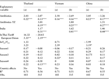
Table 2 presents the estimates of regression (7) for Vietnam, China, and Thailand. I correct the error in all cases for AR (1) autorcorrelation since the Durbin Watson is about 1 or smaller, suggesting positive autocorrelation. I report the instrumental variable (IV) estimates that are very similar to the non-IV estimates. As indicated by the theory P ^S is a reference aggregate price index for shrimp or substitutes – I use P ^S to deflate the nominal shrimp prices. One can argue about how broadly this price index should be defined. I therefore estimate regression (7) with four different price indexes: the Consumer Price Index (CPI), the Food Price Index (Food), the unit value of shrimp (prepared and less prepared, HTS 160520 and 030613) for all major trading partners (‘Shrimp I’), and the unit value of only the less prepared shrimp (HTS 030613) for these countries (‘Shrimp II’). Table 2 reports the reports with the CPI – they are similar with the other measures. Footnote ³²

Table 2.

Second-stage estimates for Vietnam, China and Thailand

$\eqalign{\tab \ln {{{{p_{{us}_{t}} /{P_{ust}^{S} }}}} \over {{{p_{{eu}_{_{t}}}/ {P_{eut}^{S}}}}}} \equals \alpha \plus \beta _{\setnum{1}} \ln {{c_{ust} } \over {c_{eut}}} \plus \beta_{\setnum{2}} \ln {{{ {{{{Y_{ust} }/ {P_{ust} }}}} \over {{{{Y_{eut} }}/ {P_{eut} }}}} \plus \beta _{\setnum{3}\! \minus\! \setnum{5}} seasons1\comma\! 3\comma\! 4 \plus u_{t}}}\cr\tab u_{t} \equals \rho u_{t \minus \setnum{1}} \plus \epsiv _{t} \cr}$

Notes:

*** Significant at 99%.

** Significant at 95%.

* Significant at 90%.

Standard errors underneath coefficient estimates.

The coefficient on relative consumption is significant at the 99% level. The estimated coefficient has the expected sign: a higher willingness to consume in one market versus another requires a lower relative price. The coefficient on relative consumption is similar across countries. The coefficient on relative income is positive for all countries, yet not significant for China.Footnote ³³ As one can see, there is a significant amount of autocorrelation with the rho coefficient between 0.5 and 0.7 and the R² varies between 0.2 and 0.1. For China, Thailand, and Vietnam, I estimate a coefficient on relative consumption that is relatively small in size, on average respectively in the order of −0.11, −0.115, or −0.085. In other words, relatively large shifts in consumption between the United States and Europe are needed to affect relative prices in a tangible way. Holding all else constant, an increase in relative consumption of about 9% or 11% is needed to decrease the shrimp price by 1%. The demand for shrimp seems to be fairly elastic (σ is on average between 9 and 11).

We are, of course, interested in whether these estimates have anything to say about the impact of the antibiotics crisis on the relative prices. Since antibiotics change export volumes that in turn are assumed to affect prices, we can get a sense of the magnitude of the impact of antibiotics on the prices by combining the impact of antibiotics on export volumes with the impact of volumes on prices. We therefore look first at the magnitude of the coefficient on the antibiotics dummy in the first-stage regression that relates the exported quantities to the tariffs and to the other variables in the model. The first-stage regression approximates the exporter's decision and thus shows how exporters redirect their exports away from Europe toward the United States in response to Europe's high food-safety standards. (I report the first-stage regression that STATA uses in order to obtain two-stage estimates in Table A1 in the Appendix.) The coefficient of the Antibiotics dummy in columns (a) has the expected positive sign. The coefficient is significant at the 99% level. To gauge the impact of the antibiotics crisis on prices, I multiply the average coefficient of relative consumption by 2.58, 2.03, and 3.05, respectively the coefficient on antibiotics for Vietnam, Thailand, and China. The antibiotics crisis may thus, on average, have had a negative impact in the order of 0.29% on the real relative prices for Vietnam and 0.23 and 0.26% for Thailand and China. All in all, in light of the fairly drastic shifts in trade patterns, this is a fairly small number. The fairly crude way in which we measure the antibiotics crisis can be partly responsible for this small effect. Note that it is not surprising that Thailand's response to the antibiotics crises is the least strong as its exports had already shrunk as it lost its preferential status and traded under a regular MFN tariff.

Now consider, on the other hand, the relatively strong impact of the tariff reduction for Thailand. The coefficient on the tariff in the first-stage regression is statistically significant at 95% and indicates that higher tariffs in Europe increase the exports to the US relative to those going to Europe. The coefficient shows a strong response in terms of the export volume leaving Europe for the United States. Multiplied by the average consumption coefficient, the impact of a 1% tariff is in the order of a 1.85% drop in the relative price. As Europe retracted Thailand's preferential tariff, Thailand's gross tariff increased from 1.045 to 1.12, an increase of 7%. Holding all else equal, a similar tariff hike would cause a drop in the US price relative to that of Europe of 12.85%.Footnote ³⁴ This represents a more than proportional reaction of the relative price of shrimp to the tariff increase in Europe, so that the relative price of shrimp in the US vs. Europe reduces by more than the actual increase in the European tariff. One should keep in mind that Thai shrimp dominate shrimp imports in the US and that we observe a strong shift of shrimp exports away from the EU to the US after the tariff increase. Moreover, shrimp exports take place through decentralized export decisions that react to worsening export conditions in Europe (the loss of the Thai preference). While it should be straightforward for shrimp exports to determine what their optimal export strategy is for a given price of shrimp in Europe and the US, it should be harder to anticipate the total effect on the price of shrimp in Europe and the US of the shifting volumes of shrimp from all exporters combined should be, which could be one explanation for the strong drop in the relative price.

One concern about running a regression such as (7) for only one country is that it may capture a change in the relative price that is common to shrimp markets for many exporting countries.Footnote ³⁵ To address this issue, I compare in the panel regression (8) the ratio of either the Thai, Vietnamese, or Chinese relative price (denoted by capital X) and the relative price for the other five countries in our sample (denoted by i). Each time, I subtract equation (4) for either Thailand, Vietnam, or China from the equations of the other five remaining countries. Needless to say, P ^S for Europe and the United States drop out in this case, and so does the relative income term.

(8)

$\ln {{{p_{usit} }/ {p_{euit} } \over {pX_{ust} /{pX_{eut}}}} }} \equals \alpha _{i} \plus \beta _{\setnum{1}} \ln {{c_{usit}/ {c_{euit}} \over {{cX_{ust} /{cX_{eut}}}}}} \plus \beta _{\setnum{2}\! \minus\! \setnum{4}} season1\comma\! 3\comma\! 4 \plus u_{it} \comma$

where X stands for either Thailand, Vietnam, or China. I allow for country effects and seasonal dummies. As the one-country regressions showed varying degrees of autocorrelation, I estimate the panel regression with generalized least squares and allow the autocorrelation coefficient to vary by panel. To instrument for the relative quantities consumed, I use the dummies for the antibiotics crisis, and a dummy for India in 1998 to capture the temporary ban on its exports to Europe. Since there is a marked difference between how Thailand, China, and Vietnam were affected by the antibiotics crisis and the rest of the sample, I include an additional antibiotics dummy AntibioticsYZ in the first stage regression. If we evaluate shrimp prices relative to Thailand, Thailand=X and AntibioticsYZ is an additional dummy for Vietnam and China. Similarly, in case we evaluate relative to China, China=X and AntibioticsYZ stands for Vietnam and Thailand, etc. Since only the European tariff for Thailand changes, I only include the Thai European tariff in the first-stage regression as an instrument – all other tariff terms will be part of the constant of the regression.

The estimation results for regression (8) in Table 3 confirm the earlier results of the single-country regressions. In all cases, the coefficient on relative consumption is negative and significant at the 99% level. Combining these estimates with the first-stage estimates of Table A1, we again find for Thailand a very strong response of relative prices to the retraction of Thailand's GSP status that is of the same order of magnitude as the one-country estimates. The retraction of the Thai preferential tariff in Europe floods the US market with Thai shrimp and increases the relative prices of other countries' shrimp exports relative to those in Thailand. The impact of the antibiotics crisis is again relatively small. Again, there is a marked difference in how China and Vietnam are impacted by the antibiotics crisis (relative to Thailand) versus the other countries. Ecuador, India, and Indonesia see their relative price increase relative to Thailand in the wake of the antibiotics crisis, whereas Vietnam and China's decreases. The results for China and Vietnam are also in line with the one-country regressions and confirm the earlier findings.

Table 3.

Second-stage estimates relative to Vietnam, relative to Thailand, and Relative to China

$\eqalign{\tab \ln {{p_{usit} }/ {p_{euit} } \over {pX_{ust} /{pX_{eut}}}} \equals \alpha _{i} \plus \beta _{\setnum{1}} \ln {{c_{usit}/ {c_{euit}} \over {{cX_{ust} /{cX_{eut}}}}} \plus \beta _{\setnum{2} \!\minus\! \setnum{4}} seasons1\comma\! 3\comma\! 4 \plus u_{it} }\cr \tab u_{it} \equals \rho _{i} u_{it \minus \setnum{1}} \plus \epsiv_{it} \cr}$

X=either Vietnam, Thailand, or China.

Notes:

*** Significant at 99%.

** Significant at 95%.

* Significant at 90%.

Standard errors underneath coefficient estimates.

5. Conclusion

In a recent article, Anderson and Van Wincoop (Reference Anderson and van Wincoop2003) argue that it is essential to consider multilateral frictions of all trading partners to better understand what determines trade flows between two countries. In other words, not only do bilateral tariffs and restrictions matter, but also changing tariffs or conditions with third countries can affect countries' bilateral trade. In arguing this way, Anderson and Van Wincoop address, in more general terms, the path-breaking question about trade creation/diversion that Viner (Reference Viner1950) had posed as the European Community emerged. My findings for the shrimp market follow this important line of research. I show specifically how the retraction of Thailand's preferential tariffs in Europe affects the bilateral trade between Thailand and the United States, even though the US tariffs do not change. Similarly, non-tariff frictions in Europe, i.e. more stringent food and safety standards, do not only directly affect bilateral trade between developing countries and Europe. They also have a non-negligible effect on the bilateral trade between the United States and these countries. Neither phenomenon, eroding preferences for developing countries and issues of international food and safety standards, is about to disappear in current and future trade liberalizations, especially when it comes to liberalizing agricultural products.

Moreover, my findings add an important dimension to the existing results by investigating the price effects that such reallocations of exports may have. I use the specific events in the shrimp market as a natural experiment to investigate the impact of tariff and non-tariff changes on international prices. I show how Europe's changing tariff policy with respect to the world's premier exporter, Thailand, did put downward pressure on the relative price in the United States versus Europe. The same is true for how the higher food-safety standards that Europe imposed affected the relative EU–US price for China, Vietnam, and Thailand. With my analysis of the shrimp market, I thus provide evidence that supports the well-established, but rarely investigated hypothesis that large countries through their trade policy can affect world prices. Moreover, as I study the impact of large countries on international goods prices, I offer a framework that strikes a balance between the more traditional notions of an integrated market with one world price and the more recent emphasis on segmented markets. Prices of internationally traded goods can be localized, yet they still will depend on policy changes in other (large) countries as exporters compare market conditions globally when they decide where to export to.

As argued, the trade policy changes overseas and their impact in the United States set the stage for the anti-dumping case against six developing countries in the United States – the largest anti-dumping case since the steel tariffs. More generally, the shrimp case casts a light on North–South relations. It illustrates the leverage that developed countries have as the main consumers of (many of) the exports from developing countries on the price that these countries receive.

Appendix

Table A1.

First-stage regressions for (a) regressions (7) for Thailand, Vietnam, China, and for (b) Regression (8) relative to Thailand, Vietnam, and China

Notes:

*** Significant at 99%.

** Significant at 95%.

* Significant at 90%.

Standard errors underneath coefficient estimates.

Footnotes

Notes:

*** Significant at 99%.

** Significant at 95%.

* Significant at 90%.

Standard errors underneath coefficient estimates.

¹ Maskus and Wilson (2001) and Baldwin (Reference Baldwin, Collins and Rodrik2000) analyze technical regulations as instruments of commercial policy in a unilateral, regional, and global trade context.

² For more information on the US shrimp industry: www.fao.org; www.shrimpnews.com; www.enaca.org (Shrimp Media Monitor); www.seafood.com; and www.globefish.org. Haby et al. (Reference Haby, Miget, Falconer and Graham2002) is a terrific survey of the industry.

³ The ability of countries to affect international prices and hence their terms of trade is at the core of the theoretical analyses of preferential trading agreements and the GATT by Bagwell and Staiger (Reference Bagwell and Staiger1999). Mclaren (Reference Mclaren, Collins and Rodrik2000) emphasizes the potential impact of standards on international prices. Mundell (Reference Mundell1964) studies the terms of trade in the context of a preferential trade agreement. Corden (Reference Corden1997) extensively discusses the ‘optimal tariff argument’ for large countries and provides many references.

⁴ Kreinin (Reference Kreinin1961) is a descriptive study of the effect of tariff changes on import prices and volumes.

⁵ For Goldberg and Knetter (Reference Goldberg and Knetter1997), product markets are segmented if the buyer and seller locations affect the terms of the transaction by more than the marginal cost of moving goods from one location to the other.

⁶ The ‘pass-through’ literature studies how exchange rate shocks affect prices of imported goods abroad. See Goldberg and Knetter (Reference Goldberg and Knetter1997) for an excellent survey.

⁷ The motivation to take the size of the shrimp harvest or catch in high-frequency studies as given derives from the significant meteorological and environmental uncertainty of shrimp farming; see Barten and Bettendorf (Reference Barten and Bettendorf1989), a much-cited reference in the agricultural economics literature.

⁸ Goldberg and Knetter (Reference Goldberg and Knetter1999) warn that the pass-through literature should not overlook the importance of trade restrictions. Directly relevant for my case, they indicate that with binding quantitative constraints in foreign markets, the local currency price that clears the market abroad can be invariant with respect to exchange rate changes. Consider for example an exporter who (with a given harvest) is forced out of the European market because of the antibiotics crisis. In this case, the law of one price will fail primarily because of the exclusionary policy (assuming it held before).

⁹ Most US production is warm-water shrimp from the Gulf of Mexico and the South Atlantic Region. Shrimp from the northwest and northeast coasts is cold-water shrimp.

¹⁰ Aggregate data are not available after 2002.

¹¹ The predominance of shrimp farming in these countries is one of the reasons why I do not investigate the impact of turtle protection devices and the impact that they had on shrimp trade. In addition, for the Western Hemisphere, the issue was resolved in 1996 before the period that I study.

¹² See Josupeti (Reference Josupeti2004).

¹³ There were no tariff changes in Japan over the period that is studied (Josupeti, Reference Josupeti2004).

¹⁴ According to Cuypers (Reference Cuypers1998), ASEAN countries have benefited most from the European Union's GSP.

¹⁵ For a chronology of the antibiotics crisis, see www.shrimpnews.com/Mitch.html.

¹⁶ See http://www.seafood.com.

¹⁷ This reportedly was the case for Indonesia and Ecuador, Shrimp Media Monitor, July 2004.

¹⁸ Obviously, if consumption and real income were expressed in dollars, which is often the case in international studies (not ours), only dollar prices would be appropriate.

¹⁹ Shrimp harvests in aquaculture (like trawling) are very dependent on ecological and meteorological circumstances. Note also that in the context of developing countries, storage technology, resources, and information to adjust production in response to prices tend to be less prevalent.

²⁰ Considering multiple markets is consistent with the pricing to market literature, see Goldberg and Knetter (Reference Goldberg and Knetter1997). Different, of course, is the given X, the focus on inverse demand curves and trade restrictions.

²¹ In the appendix of the CEPR working paper version, I specify the maximization. I provide the closed-form solution for when α_ij are the same. When α_ij are different, no such solution can be obtained (Working Paper 5254).

²² It takes seven to ten days to deliver Thai shrimp to Japan according to Seafood.com, and 20 to 30 days to deliver to the United States. Shipping Thai shrimp to Europe takes between 30 and 45 days.

²³ Note that new standards can also affect the production process and the long-term survival of firms. Relevant for us here are only those effects that in the short term directly affect the allocation decision.

²⁴ At the most disaggregate HTS level category definitions vary.

²⁵ Like the FAO, I do not rescale the quantities to shell-on headless form, since it is not clear for the various categories which weight one should apply. Haby et al. (Reference Haby, Miget, Falconer and Graham2002) recommends some weights.

²⁶ See more plots in the working version of the paper, CEPR Working Paper 5254.

²⁷ To obtain the aggregate prices, I divide the aggregate value of shrimp exports by the aggregate quantities. The 11 countries mentioned include our six countries, plus Argentina, Mexico, Brazil, the Philippines, and Malaysia. Shrimp I and Shrimp II are averages.

²⁸ To explicitly compare dollar prices in Europe and the United States, one simply multiplies through the left-hand side with the dollar–euro exchange rate and also includes it on the right-hand side of the regression. Needless to say, the outcome is the same. I need dollar–euro prices, because of how I measure quantities, prices, and real income. All of these are not expressed in dollars for Europe. Consumption is in kilogram; real income is proxied by the index of manufacturing production and the aggregate price index tracks euro prices.

²⁹ The National Marine Fisheries Service estimates that per-capita shrimp consumption increased in 1996 to 2001 by 48%. See http://www.st.nmfs.gov. Real per-capita income increased according to BLS by 10%.

³⁰ The antibiotics crisis barely registers in the media in Europe and the United States, where it could affect consumer behavior. The actual anti-dumping case will attract much more attention.

³¹ In theory, the dollar–euro exchange rate is a candidate instrument. However, as an aggregate variable, it affects income and thus demand, whereas my instruments are specific to the shrimp market and identified with a shifting supply.

³² The 11 countries include our six countries, plus Argentina, Mexico, Brazil, the Philippines, and Malaysia. The working paper version shows estimates with the other price indices.

³³ The significant Chinese seasonal dummies for fall (3) and winter (4) are responsible for the insignificant effect of relative income in the Chinese case.

³⁴ Note that the relative price on the left-hand side is inclusive of tariffs. To make sure Thailand's changing tariff with which we adjust the price index on the left-hand side is not driving the result, I have estimated the relative price regressions exclusive of the tariff. The results are very similar in all four cases.

³⁵ Using different measures for P^S already, in part, addresses this concern.

References

Anderson, Jim and van Wincoop, Eric (2003), ‘Gravity with Gravitas: A Solution to the Border Puzzle’, American Economic Review, 93: 170–192.CrossRef Google Scholar

Bagwell, Kyle and Staiger, Robert (1999), ‘An Economic Theory of GATT’, American Economic Review, 89: 215–248.CrossRef Google Scholar

Baldwin, Richard (2000), ‘Regulatory Protectionism, Developing Nations, and a Two-Tier World Trade System’, in Collins, Susan and Rodrik, Dani (eds.), Trade Forum, Washington, DC: The Brookings Institution, pp. 237–293.Google Scholar

Barten, Anton and Bettendorf, Leon (1989), ‘Price Formation of Fish – An Application of an Inverse Demand System’, European Economic Review, 33: 1509–1525.CrossRef Google Scholar

Brown, D. (1987), ‘Tariffs, the Terms of Trade and National Product Differentiation’, Journal of Policy Modeling, 3: 503–526.CrossRef Google Scholar

Chang, Won and Winters, Alan (2002), ‘How Regional Blocs Affect Excluded Countries: The Price Effects of MERCOSUR’, American Economic Review, 92: 889–904.CrossRef Google Scholar

Corden, Max (1997), Trade Policy and Economic Welfare, Oxford: Oxford University Press.CrossRef Google Scholar

Cuypers, H. (1998), ‘The Generalised System of Preferences of the European Union, with Special Reference to Asean and Thailand’, CAS Discussion Paper 18, March.Google Scholar

Debaere, Peter (2005), ‘Small Fish-Big Issues: The Effect of Trade Policy on the Global Shrimp Market’, CEPR Working Paper 5254.Google Scholar

EC Prep Monthly Report on Trade Issues in Asia Pacific (various issues).Google Scholar

EUROSTAT (2005), http://epp.eurostat.cec.eu.int.Google Scholar

Feenstra, Robert (1989), ‘Symmetric Pass-Through of Tariffs and Exchange Rates under Imperfect Competition: An Empirical Test’, Journal of International Economics, 27: 25–45.CrossRef Google Scholar

Goldberg, Pinelopi and Knetter, Michael (1997), ‘Goods Prices and Exchange Rates: What Have We Learned?’, Journal of Economic Literature, 35: 1243–1272.Google Scholar

Goldberg, Pinelopi and Knetter, Michael (1999), ‘Measuring the Intensity of Competition in Export Markets’, Journal of International Economics, 47: 27–60.CrossRef Google Scholar

Haby, Michael, Miget, Russell, Falconer, Lawrence, and Graham, Gary (2002), ‘A Review of Current Conditions in the Texas Shrimp Industry: An Examination of Contributing Factors, and Suggestions for Remaining Competitive in the Global Shrimp Market’, Working Paper, Texas A&M University.Google Scholar

Josupeti, Helga (2004), ‘Shrimp Market Access, Tariffs and Regulations’, Conference Presentation, FAO, World Shrimp Markets, October 2004, Madrid.Google Scholar

Kreinin, Mordechai (1961), ‘Effect of Tariff Changes on the Prices and Volume of Imports’, American Economic Review, 51: 310–324.Google Scholar

Maskus, Keith and Wilson, John (eds.)(2001), Quantifying the Impact of Technical Barriers to Trade: Can't it be Done? Ann Arbor: University of Michigan Press.CrossRef Google Scholar

Maskus, Keith and Wilson, John (eds.)(2001), Quantifying the Impact of Technical Barriers to Trade: Can It Be Done? Univeristy of Michigan Press.CrossRef Google Scholar

Mclaren, John (2000), ‘Comments and Discussion’, in Collins, Susan and Rodrik, Dani (eds.), Trade Forum, Washington, DC: The Brookings Institution, pp. 281–285.Google Scholar

Mundell, Robert (1964), ‘Tariff Preferences and the Terms of Trade’, Manchester School Economic Social Studies, 32: 1–13.CrossRef Google Scholar

Shrimp Media Monitoring (various issues), http://www.enaca.org.Google Scholar

OECD (2005), On-line library, http://new.sourceOECD.org.Google Scholar

Romalis, John (2005), ‘NAFTA's and CUFSTA's impact on International Trade’, NBER WP 11059.CrossRef Google Scholar

TARIC database (2005), http://europa.eu.int/comm.Google Scholar

United States International Trade Commission (2005), http://dataweb.usitc.gov.Google Scholar

Viner, J. (1950), The Customs Union Issue, New York: Carnegie Endowment.Google Scholar

Wall Street Journal (2004), ‘Catch of the Day: Battle over Shrimp’, June.Google Scholar

Figure 1. Shares of world production (percentage)

Table 1. Export quantity shares of some major shrimp producers in 1996 (percentage)

Figure 2. The shrimp market, prices, and export shares, 1996–2004

Source: USITC, EUROSTAT.

Table 2. Second-stage estimates for Vietnam, China and Thailand\eqalign{\tab \ln {{{{p_{{us}_{t}} /{P_{ust}^{S} }}}} \over {{{p_{{eu}_{_{t}}}/ {P_{eut}^{S}}}}}} \equals \alpha \plus \beta _{\setnum{1}} \ln {{c_{ust} } \over {c_{eut}}} \plus \beta_{\setnum{2}} \ln {{{ {{{{Y_{ust} }/ {P_{ust} }}}} \over {{{{Y_{eut} }}/ {P_{eut} }}}} \plus \beta _{\setnum{3}\! \minus\! \setnum{5}} seasons1\comma\! 3\comma\! 4 \plus u_{t}}}\cr\tab u_{t} \equals \rho u_{t \minus \setnum{1}} \plus \epsiv _{t} \cr}

Table 3. Second-stage estimates relative to Vietnam, relative to Thailand, and Relative to China\eqalign{\tab \ln {{p_{usit} }/ {p_{euit} } \over {pX_{ust} /{pX_{eut}}}} \equals \alpha _{i} \plus \beta _{\setnum{1}} \ln {{c_{usit}/ {c_{euit}} \over {{cX_{ust} /{cX_{eut}}}}} \plus \beta _{\setnum{2} \!\minus\! \setnum{4}} seasons1\comma\! 3\comma\! 4 \plus u_{it} }\cr \tab u_{it} \equals \rho _{i} u_{it \minus \setnum{1}} \plus \epsiv_{it} \cr} X=either Vietnam, Thailand, or China.

Table A1. First-stage regressions for (a) regressions (7) for Thailand, Vietnam, China, and for (b) Regression (8) relative to Thailand, Vietnam, and China

Article contents

Small fish–big issues: the effect of trade policy on the global shrimp market

Abstract

Information

1. The shrimp market

Thailand's changing GSP status in the European Union

AntibioticsFootnote 15

2. Model

3. Data description

4. Specification and results

5. Conclusion

Appendix

Footnotes

References

Save article to Kindle

Save article to Dropbox

Save article to Google Drive

Reply to: Submit a response

Your details

You have entered the maximum number of contributors

Conflicting interests

AntibioticsFootnote ¹⁵