1 Introduction
Turbulent fountains, formed by the continuous supply of dense fluid vertically upwards into a relatively light environment, are of considerable practical interest in the geophysical sciences and in engineering. Magma chambers replenish cyclically through the intrusion of pulses of dense magma that give rise to fountain-like flows inside the chamber (Campbell & Turner Reference Campbell and Turner1989). In low-energy building ventilation, fountains produced mechanically by the upward projection of cool air from underfloor diffusers into a warm region of a room play a key role in determining the thermal stratification, thereby influencing the comfort of occupants (Lin & Linden Reference Lin and Linden2005). Other occurrences of and practical applications for fountains that have been discussed in the literature are reviewed by Hunt & Burridge (Reference Hunt and Burridge2015).
Driven upwards by the source momentum flux, a fountain entrains ambient fluid as it first rises. The opposing buoyancy force acts to reduce the local momentum flux, and thus the fountain attains an initial maximum height
 $z=z_{in}$
above the source at
 $z=0$
before reversing direction; the upflow is then shrouded by a descending counterflow. The interaction, in the form of turbulent exchanges of momentum, between the upflow and counterflow reduces the height of the fountain which subsequently fluctuates about a mean height
 $z=z_{ss}$
. In his seminal study of saline fountains ejected vertically upwards into fresh water, Turner (Reference Turner1966) measured the initial rise height and the mean rise height and showed that they scale on the (source) momentum jet length
 $$\begin{eqnarray}L_{M}=\unicode[STIX]{x03C0}^{1/4}b_{0}Fr_{0},\end{eqnarray}$$
where
 $Fr_{0}=w_{0}/\sqrt{b_{0}g_{0}^{\prime }}$
is the source Froude number and
 $b_{0}$
,
 $w_{0}$
and
 $g_{0}^{\prime }$
are the radius, vertical velocity and buoyancy at the source, respectively. More than 40 years on, measurements by Burridge & Hunt (Reference Burridge and Hunt2013), again on aqueous-saline fountains, confirmed Turner’s (high-
 $Fr_{0}$
) result that
 $z_{in}/z_{ss}=1.43$
and revealed that the ratio of rise heights
 $z_{in}/z_{ss}$
is not invariant for lower
 $Fr_{0}$
. They also confirmed that the self-regulating double structure, comprised of an upflow and counterflow, is unique to fountains that are sufficiently ‘forced’ at their source
 $(Fr_{0}\gtrsim 3.0)$
. Rise height scalings derived theoretically by Kaye & Hunt (Reference Kaye and Hunt2006), measurements of rise height ratio (Burridge & Hunt Reference Burridge and Hunt2012) and of fountain-top fluctuations (Burridge & Hunt Reference Burridge and Hunt2013) substantiate the threshold
 $Fr_{0}\gtrsim 3.0$
. An additional class of ‘highly forced’ fountains was also identified by Burridge & Hunt (Reference Burridge and Hunt2012) for
 $Fr_{0}>5.5$
, though their established behaviour was indistinguishable from forced fountains. Notably, the current classification relies on external characteristics and is thus unable to inform us about any state of balance reached internally between the different regions of flow within a fountain. Herein, we theoretically investigate the governing dynamics in the high-
 $Fr_{0}$
limit with a view to enhancing the current understanding of when a fountain may be regarded as a forced fountain, paying particular attention to the notion of self-preservation within a fountain.
A model of the upflow prior to the formation of a counterflow developed by Morton (Reference Morton1959) has paved the way for a classification of fountains (Kaye & Hunt Reference Kaye and Hunt2006), analytical solutions for fountains in linearly stratified environments (Mehaddi, Vauquelin & Candelier Reference Mehaddi, Vauquelin and Candelier2012) and more complex models for steady forced fountains that account for interactions once the counterflow has formed (McDougall Reference Mcdougall1981; Bloomfield & Kerr Reference Bloomfield and Kerr2000). Owing to the scarcity of experimental data on the complex turbulent exchanges between the upflow and counterflow, these interactions are not fully understood. As a consequence, the ideas of Morton (Reference Morton1962) on entrainment between two turbulent flows are central to the parameterisation of the fluxes exchanged between the upflow and counterflow. Alternative formulations seek to account for the counterflow implicitly by calibrating shape parameters to experimental measurements (Carazzo, Kaminski & Tait Reference Carazzo, Kaminski and Tait2010) or to numerical simulations (Mehaddi et al. Reference Mehaddi, Vaux, Candelier and Vauquelin2015).
Surprisingly, nearly all modellers have ignored the region of flow reversal at the top of the fountain, where the action of the buoyancy effects a change in the sign of the local momentum flux. Instead, a requirement underlying previous models is that the flow reverses instantaneously at the height where the vertical (upward) velocity has reduced to zero. Such immediate reversal must be questioned as somewhat artificial. Omitting to assign a finite vertical extent to the flow-reversal region, whilst physically unrealistic, also leads to unboundedness: as the velocity reduces to zero close to the fountain top, conservation of mass flux dictates that the radius tends to infinity. Thus, as a consequence of neglecting to model the fountain top appropriately, systematic discrepancies are observed between model predictions and measurements close to the top. Although McDougall (Reference Mcdougall1981) offers a (non-entraining) model for this region, which he apportions into two zones, of which one is modelled as a cylinder, questions regarding its appropriateness remain open. For example, experimental observations indicate that the radius of the upflow varies rapidly with height near the top. Moreover, the McDougall model requires an ad hoc assumption of the cylinder’s vertical extent, which in turn influences directly the predictions of rise height. Pertinently, all current models neglect fountain-top entrainment, while experimental and numerical results suggest that entrainment plays an instrumental role in the dilution of buoyant fluid as it reverses direction (Lin & Linden Reference Lin and Linden2005; Devenish, Rooney & Thomson Reference Devenish, Rooney and Thomson2010). Furthermore, as the fluxes leaving the flow reversal region prescribe the ‘starting’ conditions for the counterflow, and may therefore modulate the exchanges between counterflow and upflow (cf. Morton Reference Morton1962), it is imperative that this region is well modelled and its effects better quantified.
Fuelled by the aim of providing a more complete theoretical description of high-Froude number fountains, in § 2 we present a model for a time-averaged turbulent axisymmetric forced fountain characterised by an upflow, a counterflow, and an entraining fountain top where the flow reverses direction. This new approach, which bounds the flow both vertically and radially, enables the prediction of the fountain envelope over its whole extent. The conservation equations are expressed in terms of Froude numbers for the upflow and counterflow
 $(Fr_{u},Fr_{c})$
so that their solutions provide direct insight into the local fountain behaviour at all heights. In § 3, we illustrate the close agreement of our solutions with existing experimental data. The robustness of the three-region model is assessed in § 4, where we implement an alternative formulation for the body forces acting on the fountain and compare the predictions for both formulations. Drawing on the key results from our model, we conclude in § 5 by suggesting when a continuous negatively buoyant release of fluid may be regarded as giving rise to a forced fountain.
2 Theoretical model
We restrict our attention to turbulent fountains formed by a continuous and steady supply of dense fluid forced vertically upwards from a circular source into a relatively light quiescent uniform environment. Based on the findings of Williamson et al. (Reference Williamson, Srinarayana, Armfield, Mcbain and Lin2008) and Burridge, Mistry & Hunt (Reference Burridge, Mistry and Hunt2015), we anticipate that this requires the source Reynolds number
 $Re_{0}=w_{0}b_{0}/\unicode[STIX]{x1D708}>2000$
, where
 $\unicode[STIX]{x1D708}$
designates the kinematic velocity of the source fluid. Denoting the densities of the source fluid as
 $\unicode[STIX]{x1D70C}_{0}$
and the environment as
 $\unicode[STIX]{x1D70C}_{a}<\unicode[STIX]{x1D70C}_{0}$
, the source fluid experiences a buoyancy
 $$\begin{eqnarray}g_{0}^{\prime }=g\left(\frac{\unicode[STIX]{x1D70C}_{0}-\unicode[STIX]{x1D70C}_{a}}{\unicode[STIX]{x1D70C}_{a}}\right),\end{eqnarray}$$
where
 $g$
is the acceleration due to gravity. Our focus lies on Boussinesq releases, for which
 $\unicode[STIX]{x1D70C}_{0}-\unicode[STIX]{x1D70C}_{a}\ll \unicode[STIX]{x1D70C}_{a}$
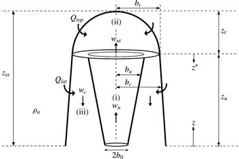
. In our time-averaged conceptualisation, we model the quasi-steady axisymmetric fountain by considering three flow regions that characterise its behaviour, as depicted in figure 1: (i) a negatively buoyant upflowing jet-like core of density
 $\unicode[STIX]{x1D70C}_{u}>\unicode[STIX]{x1D70C}_{a}$
, (ii) a fountain top where the flow reverses direction and (iii) an annular negatively buoyant counterflowing plume-like flow of density
 $\unicode[STIX]{x1D70C}_{c}>\unicode[STIX]{x1D70C}_{a}$
(the subscripts ‘
 $u$
’ and ‘
 $c$
’ read ‘upflow’ and ‘counterflow’, respectively).
For simplicity, we do not attempt to model the complex variations in cross-stream profiles evident from measurements (e.g. Mizushina et al.
Reference Mizushina, Ogino, Takeuchi and Ikawa1982) and model the upflow and the counterflow as being described by a single density at each height so that
 $\unicode[STIX]{x1D70C}_{u}=\unicode[STIX]{x1D70C}_{u}(z)$
and
 $\unicode[STIX]{x1D70C}_{c}=\unicode[STIX]{x1D70C}_{c}(z)$
. As a consequence, we choose top-hat profiles within the upflow and the counterflow for the time-averaged horizontal variation of vertical velocities,
 $w_{u}$
and
 $w_{c}$
(defined to be positive in the direction of mean flow, i.e. upwards in the upflow and downwards in the counterflow, figure 1), and for the buoyancies
 $$\begin{eqnarray}g_{u}^{\prime }=g\left(\frac{\unicode[STIX]{x1D70C}_{u}-\unicode[STIX]{x1D70C}_{a}}{\unicode[STIX]{x1D70C}_{a}}\right),\quad g_{c}^{\prime }=g\left(\frac{\unicode[STIX]{x1D70C}_{c}-\unicode[STIX]{x1D70C}_{a}}{\unicode[STIX]{x1D70C}_{a}}\right).\end{eqnarray}$$
Herein (§ 3), we show that good agreement between our predictions and measurements (specifically of rise height, upflow and counterflow radii and velocities) is obtained on adopting top-hat profiles. Whilst we make no explicit claim regarding the self-similarity of cross-stream profiles, our simplification is consistent with this notion. The assumption of self-similar profiles of vertical velocity and buoyancy across each horizontal section of the flow has been questioned in light of experimental results (Mizushina et al. Reference Mizushina, Ogino, Takeuchi and Ikawa1982). Nevertheless, models developed under the assumption of self-similarity have been successful in capturing the bulk behaviour of flows that are not fully self-similar, such as the near source flow of forced plumes, lazy plumes and indeed fountains.
Schematic and notation for the time-averaged turbulent fountain. The fountain source, of radius
 $b_{0}$
, is located at
 $z=0$
. The fountain is characterised by three regions: (i) upflow, (ii) fountain top with entrainment
 $Q_{top}$
(
 $\text{m}^{3}~\text{s}^{-1}$
) and (iii) counterflow with entrainment
 $Q_{lat}$
(
 $\text{m}^{3}~\text{s}^{-1}$
).

Guided by the observations of Turner (Reference Turner1966) and the detailed measurements of Mizushina et al. (Reference Mizushina, Ogino, Takeuchi and Ikawa1982), we further assume that the total fountain radius,
 $b_{c}$
, remains constant with height. As we will see in § 2.3, this considerably simplifies the analysis of the counterflow without significantly affecting our predictions (cf. appendix A).
Turbulent entrainment at the lateral perimeter between the fountain and the ambient gives rise to the lateral entrainment flux
 $Q_{lat}$
of ambient fluid into the counterflow (figure 1). Turbulent entrainment also maintains a continuous exchange of fluxes between the two counterflowing streams. The lack of detailed measurements on this complex exchange compounds the challenge of quantifying the interactions between the upflow and the counterflow. Thus, in the absence of data to support a more complex entrainment model, we parameterise the entrainment into the upflow and into the counterflow using the classic entrainment hypothesis of Morton, Taylor & Turner (Reference Morton, Taylor and Turner1956), i.e. by assuming that, at a given height, the horizontal entrainment velocity into the upflow is proportional to the upward velocity
 $w_{u}$
, and the horizontal entrainment velocity into the counterflow is proportional to the downward velocity
 $w_{c}$
. This formulation provides an insight into the dominant direction of entrainment, i.e. whether fluid is transported primarily from the counterflow into the upflow or vice versa. As the upflow exhibits jet-like behaviour over a significant fraction of its rise height
 $z_{u}$
, the largest vertical velocities are primarily associated with the upflow, that is
 $w_{u}\gg w_{c}$
. Indeed, the Bloomfield & Kerr (Reference Bloomfield and Kerr2000) model indicates that over a jet length
 $L_{M}$
(1.1) the velocity ratio
 $w_{u}/w_{c}\gg 5$
. Therefore, anticipating that transport of fluid into the upflow is dominant, we neglect entrainment from the upflow into the counterflow. Consistent with this approximation, Bloomfield & Kerr found that entrainment from the upflow into the counterflow has a relatively minor influence on the dynamics.
2.1 Upflowing jet core
Assuming an incompressible flow, conservation of volume for the upflow requires
 $$\begin{eqnarray}\frac{\text{d}Q_{u}}{\text{d}z}=2\unicode[STIX]{x03C0}b_{u}(\unicode[STIX]{x1D6FC}_{u}w_{u}),\end{eqnarray}$$
where
 $\unicode[STIX]{x1D6FC}_{u}=u_{eu}/w_{u}$
is the top-hat entrainment coefficient for the upflow and
 $u_{eu}$
denotes the horizontal entrainment velocity into the upflow. Notably, whilst several studies report estimates of
 $\unicode[STIX]{x1D6FC}_{u}$
for the initial upflow, there is no general consensus on an appropriate value for
 $\unicode[STIX]{x1D6FC}_{u}$
once the counterflow has formed. By treating the upflow as a momentum-driven jet, Burridge & Hunt (Reference Burridge and Hunt2013) used their measurements of the rise height of the upflow and its radius near the top to estimate a value of
 $\unicode[STIX]{x1D6FC}_{u}=0.0425$
based on the spreading rate. This is lower than the value of
 $\unicode[STIX]{x1D6FC}_{u}=0.075$
reported by Williamson, Armfield & Lin (Reference Williamson, Armfield and Lin2011) from their numerical simulations of forced fountains. Herein, we take
 $\unicode[STIX]{x1D6FC}_{u}=0.06$
, corresponding approximately to the mid-value of the range of these two studies.
To this day relatively little is known about the internal dynamics of a fountain. In particular, lacking knowledge of the interaction between the upflow and the counterflow makes it daunting to specify the exchange of momentum between the two flows. In this section, we opt for a simple yet powerful formulation that follows naturally from the ideas of Morton (Reference Morton1962). We will return to the formulation of body forces acting on the fountain in § 4.
We consider a control volume of height
 $\text{d}z$
around the upflow. Assuming that the pressure is hydrostatic throughout the fountain and given that the fluxes of momentum
 $(\propto \unicode[STIX]{x1D70C}_{u}b_{u}^{2}w_{u}^{2})$
entering and exiting this control volume at heights
 $z$
and
 $z+\text{d}z$
, respectively, are positive in the positive
 $z$
-direction (figure 1), conservation of vertical momentum requires
 $$\begin{eqnarray}[\unicode[STIX]{x03C0}\unicode[STIX]{x1D70C}_{u}b_{u}^{2}w_{u}^{2}]_{z+\text{d}z}-[\unicode[STIX]{x03C0}\unicode[STIX]{x1D70C}_{u}b_{u}^{2}w_{u}^{2}]_{z}+2\unicode[STIX]{x03C0}\unicode[STIX]{x1D70C}_{c}b_{u}u_{eu}w_{c}\,\text{d}z=-\unicode[STIX]{x03C0}\unicode[STIX]{x1D70C}_{a}b_{u}^{2}g_{u}^{\prime }\,\text{d}z,\end{eqnarray}$$
where the third term represents the flux of downward momentum entrained into the upflow from the counterflow. The right-hand side of (2.4) represents the buoyancy force acting downward on the upflow. Similarly, given that the fluxes of buoyancy
 $(\propto b_{u}^{2}w_{u}g_{u}^{\prime })$
entering and exiting the control volume at heights
 $z$
and
 $z+\text{d}z$
are negative in the positive
 $z$
-direction, conservation of buoyancy requires
 $$\begin{eqnarray}-[\unicode[STIX]{x03C0}b_{u}^{2}w_{u}g_{u}^{\prime }]_{z}-2\unicode[STIX]{x03C0}b_{u}u_{eu}g_{c}^{\prime }\,\text{d}z=-[\unicode[STIX]{x03C0}b_{u}^{2}w_{u}g_{u}^{\prime }]_{z+dz},\end{eqnarray}$$
where the second term is the negative buoyancy flux entrained from the counterflow into the upflow. Thus, from (2.4) and (2.5), the vertical rate of change of the specific momentum flux
 $M_{u}=\unicode[STIX]{x03C0}b_{u}^{2}w_{u}^{2}$
and specific buoyancy flux
 $B_{u}=\unicode[STIX]{x03C0}b_{u}^{2}w_{u}g_{u}^{\prime }$
for the upflow are
 $$\begin{eqnarray}\frac{\text{d}M_{u}}{\text{d}z}=-\unicode[STIX]{x03C0}b_{u}^{2}g_{u}^{\prime }-2\unicode[STIX]{x03C0}b_{u}w_{c}(\unicode[STIX]{x1D6FC}_{u}w_{u}),\quad \frac{\text{d}B_{u}}{\text{d}z}=2\unicode[STIX]{x03C0}b_{u}g_{c}^{\prime }(\unicode[STIX]{x1D6FC}_{u}w_{u}),\end{eqnarray}$$
for Boussinesq flows.
Scaling quantities of interest on their values at the fountain source
 $(z=0)$
, for the upflow we introduce the dimensionless radius
 $\unicode[STIX]{x1D6FD}_{u}$
, dimensionless vertical velocity
 $\unicode[STIX]{x1D714}_{u}$
and Froude number
 $Fr_{u}$
 $$\begin{eqnarray}\unicode[STIX]{x1D6FD}_{u}=\frac{b_{u}}{b_{0}},\quad \unicode[STIX]{x1D714}_{u}=\frac{w_{u}}{w_{0}},\quad Fr_{u}=\frac{w_{u}}{\sqrt{b_{u}g_{u}^{\prime }}},\quad \unicode[STIX]{x1D709}=\frac{6\unicode[STIX]{x1D6FC}_{u}}{5}\frac{z}{b_{0}},\end{eqnarray}$$
where
 $\unicode[STIX]{x1D709}$
is the dimensionless vertical coordinate. The scaling for
 $z$
is chosen so that in the absence of a counterflow, we recover the non-dimensional conservation equations of Kaye & Hunt (Reference Kaye and Hunt2006) describing the initial rise of the upflow. For the counterflow, the dimensionless radius
 $\unicode[STIX]{x1D6FD}_{c}$
, dimensionless vertical velocity
 $\unicode[STIX]{x1D714}_{c}$
and Froude number
 $Fr_{c}$
are
 $$\begin{eqnarray}\unicode[STIX]{x1D6FD}_{c}=\frac{b_{c}}{b_{0}},\quad \unicode[STIX]{x1D714}_{c}=\frac{w_{c}}{w_{0}},\quad Fr_{c}=\frac{w_{c}}{\sqrt{(b_{c}^{2}-b_{u}^{2})^{1/2}g_{c}^{\prime }}}.\end{eqnarray}$$
Defining the non-dimensional fluxes of volume
 $q_{u}$
, momentum
 $m_{u}$
and buoyancy
 $f_{u}$
as
 $$\begin{eqnarray}q_{u}=\unicode[STIX]{x1D6FD}_{u}^{2}\unicode[STIX]{x1D714}_{u},\quad m_{u}=\unicode[STIX]{x1D6FD}_{u}^{2}\unicode[STIX]{x1D714}_{u}^{2},\quad f_{u}=Fr_{0}^{2}\unicode[STIX]{x1D714}_{u}^{3}\unicode[STIX]{x1D6FD}_{u}/Fr_{u}^{2},\end{eqnarray}$$
the conservation equations (2.3) and (2.6) become
 $$\begin{eqnarray}\displaystyle \frac{\text{d}q_{u}}{\text{d}\unicode[STIX]{x1D709}}=\frac{5}{3}\unicode[STIX]{x1D6FD}_{u}\unicode[STIX]{x1D714}_{u},\quad \frac{\text{d}m_{u}}{\text{d}\unicode[STIX]{x1D709}}=-\frac{5}{6\unicode[STIX]{x1D6FC}_{u}}\frac{\unicode[STIX]{x1D6FD}_{u}\unicode[STIX]{x1D714}_{u}^{2}}{Fr_{u}^{2}}-\frac{5}{3}\unicode[STIX]{x1D6FD}_{u}\unicode[STIX]{x1D714}_{u}\unicode[STIX]{x1D714}_{c},\quad \frac{\text{d}f_{u}}{\text{d}\unicode[STIX]{x1D709}}=\frac{5}{3}\frac{Fr_{0}^{2}}{Fr_{c}^{2}}\frac{\unicode[STIX]{x1D6FD}_{u}\unicode[STIX]{x1D714}_{u}\unicode[STIX]{x1D714}_{c}^{2}}{\sqrt{(\unicode[STIX]{x1D6FD}_{c}^{2}-\unicode[STIX]{x1D6FD}_{u}^{2})}}. & & \displaystyle \nonumber\\ \displaystyle & & \displaystyle\end{eqnarray}$$
We seek the vertical variation of upflow radius, velocity and Froude number. Differentiating
 $\unicode[STIX]{x1D6FD}_{u}=q_{u}/m_{u}^{1/2}$
,
 $\unicode[STIX]{x1D714}_{u}=m_{u}/q_{u}$
and
 $Fr_{u}=Fr_{0}m_{u}^{5/4}/(q_{u}f_{u}^{1/2})$
with respect to height gives
 $$\begin{eqnarray}\frac{\text{d}\unicode[STIX]{x1D6FD}_{u}}{\text{d}\unicode[STIX]{x1D709}}=\frac{1}{\unicode[STIX]{x1D6FD}_{u}\unicode[STIX]{x1D714}_{u}}\frac{\text{d}q_{u}}{\text{d}\unicode[STIX]{x1D709}}-\frac{1}{2}\frac{1}{\unicode[STIX]{x1D6FD}_{u}\unicode[STIX]{x1D714}_{u}^{2}}\frac{\text{d}m_{u}}{\text{d}\unicode[STIX]{x1D709}},\quad \frac{\text{d}\unicode[STIX]{x1D714}_{u}}{\text{d}\unicode[STIX]{x1D709}}=\frac{1}{\unicode[STIX]{x1D6FD}_{u}^{2}\unicode[STIX]{x1D714}_{u}}\frac{\text{d}m_{u}}{\text{d}\unicode[STIX]{x1D709}}-\frac{1}{\unicode[STIX]{x1D6FD}_{u}^{2}}\frac{\text{d}q_{u}}{\text{d}\unicode[STIX]{x1D709}},\end{eqnarray}$$
 $$\begin{eqnarray}\frac{\text{d}Fr_{u}}{\text{d}\unicode[STIX]{x1D709}}=\frac{5}{4}\frac{Fr_{u}}{\unicode[STIX]{x1D6FD}_{u}^{2}\unicode[STIX]{x1D714}_{u}^{2}}\frac{\text{d}m_{u}}{\text{d}\unicode[STIX]{x1D709}}-\frac{Fr_{u}}{\unicode[STIX]{x1D6FD}_{u}^{2}\unicode[STIX]{x1D714}_{u}}\frac{\text{d}q_{u}}{\text{d}\unicode[STIX]{x1D709}}-\frac{1}{2}\frac{Fr_{u}^{3}}{Fr_{0}^{2}}\frac{1}{\unicode[STIX]{x1D6FD}_{u}\unicode[STIX]{x1D714}_{u}^{3}}\frac{\text{d}f_{u}}{\text{d}\unicode[STIX]{x1D709}}.\end{eqnarray}$$
Finally, substituting (2.10) into (2.11) and (2.12) yields our governing system of equations
 $$\begin{eqnarray}\frac{\text{d}\unicode[STIX]{x1D6FD}_{u}}{\text{d}\unicode[STIX]{x1D709}}=\frac{5}{3}\left(1+\frac{1}{4\unicode[STIX]{x1D6FC}_{u}}\frac{1}{Fr_{u}^{2}}\right)+I_{1},\quad \frac{\text{d}\unicode[STIX]{x1D714}_{u}}{\text{d}\unicode[STIX]{x1D709}}=-\frac{5}{3}\frac{\unicode[STIX]{x1D714}_{u}}{\unicode[STIX]{x1D6FD}_{u}}\left(1+\frac{1}{2\unicode[STIX]{x1D6FC}_{u}}\frac{1}{Fr_{u}^{2}}\right)+I_{2}\end{eqnarray}$$
and
 $$\begin{eqnarray}\frac{\text{d}Fr_{u}}{\text{d}\unicode[STIX]{x1D709}}=-\frac{5}{3}\frac{Fr_{u}}{\unicode[STIX]{x1D6FD}_{u}}\left(1+\frac{5}{8\unicode[STIX]{x1D6FC}_{u}}\frac{1}{Fr_{u}^{2}}\right)+I_{3},\end{eqnarray}$$
where the ‘interaction’ terms that account for the entrainment of fluid from the counterflow into the upflow are
 $$\begin{eqnarray}I_{1}=\frac{5}{6}\frac{\unicode[STIX]{x1D714}_{c}}{\unicode[STIX]{x1D714}_{u}},\quad I_{2}=-\frac{5}{3}\frac{\unicode[STIX]{x1D714}_{c}}{\unicode[STIX]{x1D6FD}_{u}},\quad I_{3}=-\frac{5}{3}\frac{Fr_{u}}{\unicode[STIX]{x1D6FD}_{u}}\frac{\unicode[STIX]{x1D714}_{c}}{\unicode[STIX]{x1D714}_{u}}\left(\frac{5}{4}+\frac{1}{2}\frac{\unicode[STIX]{x1D714}_{c}\unicode[STIX]{x1D6FD}_{u}Fr_{u}^{2}}{\unicode[STIX]{x1D714}_{u}\unicode[STIX]{x1D6FD}_{a}Fr_{c}^{2}}\right),\end{eqnarray}$$
and
 $\unicode[STIX]{x1D6FD}_{a}=(\unicode[STIX]{x1D6FD}_{c}^{2}-\unicode[STIX]{x1D6FD}_{u}^{2})^{1/2}$
. In the absence of a counterflow
 $I_{1}=I_{2}=I_{3}=0$
and (2.13)–(2.14) reduce to the classic plume equations, albeit with negative buoyancy (cf. appendix B). The source conditions for the fountain upflow are those of the fountain source, namely
 $$\begin{eqnarray}\unicode[STIX]{x1D6FD}_{u}(\unicode[STIX]{x1D709}=0)=1,\quad \unicode[STIX]{x1D714}_{u}(\unicode[STIX]{x1D709}=0)=1,\quad Fr_{u}(\unicode[STIX]{x1D709}=0)=Fr_{0}.\end{eqnarray}$$
Recasting the conservation equations (2.10) into a form that expresses the vertical variation of the upflow Froude number
 $Fr_{u}$
(2.13)–(2.14) allows us to capture the fountain behaviour at all heights through a single dimensionless parameter (namely
 $Fr_{u}$
for the upflow and
 $Fr_{c}$
for the counterflow). This is akin to the approach developed by Hunt & Kaye (Reference Hunt and Kaye2005) for lazy plumes, where the variation of the plume with height was expressed in terms of a local Richardson number
 $\unicode[STIX]{x1D6E4}\propto Fr_{u}^{-2}$
. Based on the value of
 $Fr_{u}$
at a given height, following Kaye & Hunt (Reference Kaye and Hunt2006) the fountain can be locally classified into either (i) a ‘forced regime’ in which the flow is momentum-driven, (ii) a ‘weak regime’ in which the flow is dominated by its buoyancy or (iii) an ‘intermediate regime’ which captures the transition between the forced and weak behaviours. From the experimental measurements of saline fountains reported by Burridge & Hunt (Reference Burridge and Hunt2012), we expect these regimes to correspond to regions where (i)
 $Fr_{u}\gtrsim 2.8$
, (ii)
 $Fr_{u}\lesssim 1.4$
and (iii)
 $1.4\lesssim Fr_{u}\lesssim 2.8$
, respectively.
2.2 Flow reversal region – fountain top
The buoyancy-dominated region of flow reversal is characterised by a domed cap – the fountain top. A similar dome-like flow dominated by its buoyancy results from a weakly energetic impingement of a turbulent jet on a density interface (Shy Reference Shy1995; Cotel et al.
Reference Cotel, Gjestvang, Ramkhelawan and Breidenthal1997). Notably, external fluid is entrained into both the fountain top and the interfacial dome. For the latter, Shrinivas & Hunt (Reference Shrinivas and Hunt2014) proposed a model whereby ambient fluid is drawn into the dome in a quasi-steady manner by sustained baroclinic eddies. By combining conservation equations with a mechanistic model of entrainment into the dome, they showed that the dome is hemispherical when the Froude number at the interface
 $Fr_{i}$
, indicative of the balance between inertial and gravitational forces within the dome, takes a value of
 $Fr_{i}=1.4$
.
Although the entraining mechanism is arguably different in the fountain top, where we expect the fluctuations to play a dominant role in engulfing ambient fluid, in Debugne & Hunt (Reference Debugne and Hunt2016) we show that the Shrinivas & Hunt (Reference Shrinivas and Hunt2014) model provides a suitable description of the time-averaged entrainment into the cap. Hence, herein we model the fountain top as a hemispherical dome (figure 1), forming at height
 $z=z_{u}$
where the upflow Froude number takes a local value of
 $Fr_{u}=Fr_{ut}=1.4$
(the subscript ‘
 $t$
’ signifying the fountain top). The threshold choice of
 $Fr_{ut}=1.4$
, which stems from the analysis of Shrinivas & Hunt, finds immediate physical justification in the context of forced fountains. Indeed,
 $Fr_{ut}=1.4$
represents a tipping point where the (downward) velocity induced by gravity starts to exceed the (upward) velocity of the fountain core,
 $w_{u}$
. On physical grounds, it too seems reasonable that this value should mark the onset of flow reversal.
For the fountain top of radius
 $b_{t}$
and height
 $z_{t}=b_{t}$
, conservation of volume and vertical momentum requires
 $$\begin{eqnarray}\unicode[STIX]{x03C0}b_{ut}^{2}w_{ut}+Q_{top}=\unicode[STIX]{x03C0}(b_{t}^{2}-b_{ut}^{2})w_{t},\quad \unicode[STIX]{x03C0}\unicode[STIX]{x1D70C}_{ut}b_{ut}^{2}w_{ut}^{2}+\unicode[STIX]{x03C0}\unicode[STIX]{x1D70C}_{t}(b_{t}^{2}-b_{ut}^{2})w_{t}^{2}=\frac{2\unicode[STIX]{x03C0}}{3}\unicode[STIX]{x1D70C}_{ut}g_{ut}^{\prime }b_{t}^{3}.\end{eqnarray}$$
Here,
 $b_{ut}$
,
 $w_{ut}$
,
 $\unicode[STIX]{x1D70C}_{ut}$
and
 $g_{ut}^{\prime }$
designate the radius, vertical velocity, density and buoyancy of the upflow at
 $z=z_{u}$
, respectively, and
 $Q_{top}$
denotes the volume flux entrained through the fountain cap; finally,
 $\unicode[STIX]{x1D70C}_{t}$
and
 $w_{t}$
are the density and (magnitude of the) velocity of the outflow from the fountain top. In (2.17a
), the volume flux supplied by the upflow to the fountain top and the volume flux
 $Q_{top}$
entrained into the fountain top are balanced by the flux of volume leaving the fountain top. Similarly, in (2.17b
), the fluxes of momentum into (first term) and out of (second term) the fountain top are balanced by the opposing buoyancy force (right-hand side) acting on the dense fluid within the fountain top. Substituting for
 $w_{t}^{2}$
from (2.17a
) into (2.17b
) and making the Boussinesq approximation yields a polynomial in the dimensionless fountain-top radius
 $\unicode[STIX]{x1D6FD}_{t}=b_{t}/b_{0}$
:
 $$\begin{eqnarray}\frac{2\unicode[STIX]{x1D6FD}_{t}^{5}}{Fr_{ut}^{2}\unicode[STIX]{x1D6FD}_{ut}^{5}}-\frac{2\unicode[STIX]{x1D6FD}_{t}^{3}}{Fr_{ut}^{2}\unicode[STIX]{x1D6FD}_{ut}^{3}}-\frac{3\unicode[STIX]{x1D6FD}_{t}^{2}}{\unicode[STIX]{x1D6FD}_{ut}^{2}}-3E_{top}(E_{top}+2)=0,\quad E_{top}=\frac{Q_{top}}{\unicode[STIX]{x03C0}b_{ut}^{2}w_{ut}},\end{eqnarray}$$
where
 $\unicode[STIX]{x1D6FD}_{ut}=b_{ut}/b_{0}$
. Note that the variables with a subscript ‘
 $t$
’ (figure 1, (2.17)–(2.18)) are also those pertinent to the top of the counterflow, i.e.
 $b_{t}\equiv b_{ct}$
,
 $w_{t}\equiv w_{ct}$
,
 $\unicode[STIX]{x1D70C}_{t}\equiv \unicode[STIX]{x1D70C}_{ct}$
, so that the solution of (2.18) gives the radius of the counterflow at its top. As discussed at length in Debugne & Hunt (Reference Debugne and Hunt2016), we follow Shrinivas & Hunt (Reference Shrinivas and Hunt2014) in taking
 $E_{top}=0.525$
for
 $Fr_{ut}=1.4$
. This is within the range
 $0.5<E_{top}<0.8$
reported by Lin & Linden (Reference Lin and Linden2005). As will be shown in § 3, lateral entrainment into the counterflow is dominant in forced fountains, so that the choice of
 $E_{top}$
within this range has a relatively minor influence on our predictions. Equally, our solutions are relatively insensitive to
 $Fr_{ut}$
. For example, decreasing
 $Fr_{ut}=1.4$
to
 $Fr_{ut}=1$
increases the fountain’s rise height by 2 % (note that
 $E_{top}=0.25$
for
 $Fr_{ut}=1$
, Shrinivas & Hunt Reference Shrinivas and Hunt2014).
Conservation of buoyancy for the fountain top requires
 $$\begin{eqnarray}\unicode[STIX]{x03C0}(b_{t}^{2}-b_{ut}^{2})w_{t}g_{t}^{\prime }=\unicode[STIX]{x03C0}b_{ut}^{2}w_{ut}g_{ut}^{\prime },\quad g_{t}^{\prime }=g(\unicode[STIX]{x1D70C}_{t}-\unicode[STIX]{x1D70C}_{a})/\unicode[STIX]{x1D70C}_{a}.\end{eqnarray}$$
Non-dimensionalising (2.17a
) and (2.19) gives the dimensionless vertical velocity
 $\unicode[STIX]{x1D714}_{t}=w_{t}/w_{0}$
and Froude number
 $Fr_{t}$
of the downflow from the fountain top as
 $$\begin{eqnarray}\unicode[STIX]{x1D714}_{t}=\frac{\unicode[STIX]{x1D6FD}_{ut}^{2}\unicode[STIX]{x1D714}_{ut}(1+E_{top})}{\unicode[STIX]{x1D6FD}_{t}^{2}-\unicode[STIX]{x1D6FD}_{ut}^{2}},\quad Fr_{t}=\frac{w_{t}}{\sqrt{(b_{t}^{2}-b_{ut}^{2})^{1/2}g_{t}^{\prime }}}=Fr_{ut}\left\{\frac{\unicode[STIX]{x1D714}_{t}^{3}\sqrt{\unicode[STIX]{x1D6FD}_{t}^{2}-\unicode[STIX]{x1D6FD}_{ut}^{2}}}{\unicode[STIX]{x1D714}_{ut}^{3}\unicode[STIX]{x1D6FD}_{ut}}\right\}^{1/2}.\end{eqnarray}$$
Together with
 $\unicode[STIX]{x1D6FD}_{t}$
from (2.18),
 $\unicode[STIX]{x1D714}_{t}$
and
 $Fr_{t}$
from (2.20) describe the initial condition for the counterflow in terms of radius, velocity and Froude number at the exit of the fountain top.
2.3 Counterflow
To complete our three-region model, it is necessary to describe the counterflow. For convenience, we define a vertical downward coordinate
 $z^{\ast }$
with origin at the base of the fountain top (figure 1). Noting that the vertical velocity of the counterflow and the buoyancy fluxes of the upflow and counterflow are positive in the positive
 $z^{\ast }$
-direction, conservation of volume flux
 $Q_{c}=\unicode[STIX]{x03C0}(b_{c}^{2}-b_{u}^{2})w_{c}$
and buoyancy flux
 $B_{c}=g_{c}^{\prime }Q_{c}$
for the counterflow requires
 $$\begin{eqnarray}\frac{\text{d}Q_{c}}{\text{d}z^{\ast }}=2\unicode[STIX]{x03C0}b_{c}(\unicode[STIX]{x1D6FC}_{c}w_{c})-2\unicode[STIX]{x03C0}b_{u}(\unicode[STIX]{x1D6FC}_{u}w_{u}),\quad \frac{\text{d}B_{c}}{\text{d}z^{\ast }}=-2\unicode[STIX]{x03C0}b_{u}g_{c}^{\prime }(\unicode[STIX]{x1D6FC}_{u}w_{u}),\end{eqnarray}$$
where
 $\unicode[STIX]{x1D6FC}_{c}$
denotes the entrainment coefficient for the counterflow. Numerical simulations performed by Williamson et al. (Reference Williamson, Armfield and Lin2011) suggest
 $0.1<\unicode[STIX]{x1D6FC}_{c}<0.2$
and herein we take
 $\unicode[STIX]{x1D6FC}_{c}=0.15$
, the mid-value of their range. This is close to the value in line plumes reported by Kotsovinos & List (Reference Kotsovinos and List1977) (
 $\unicode[STIX]{x1D6FC}_{lp}=0.147\pm 0.014$
) and, indeed, identical to the model value of Bloomfield & Kerr (Reference Bloomfield and Kerr2000). We invoke the assumption that the total fountain diameter
 $2b_{c}$
is constant with height and non-dimensionalise (2.21a
) to obtain
 $$\begin{eqnarray}\frac{\text{d}\unicode[STIX]{x1D714}_{c}}{\text{d}\unicode[STIX]{x1D709}^{\ast }}=\frac{5}{3\unicode[STIX]{x1D6FD}_{a}^{2}}\left\{\frac{\unicode[STIX]{x1D6FC}_{c}}{\unicode[STIX]{x1D6FC}_{u}}\unicode[STIX]{x1D6FD}_{c}\unicode[STIX]{x1D714}_{c}-\unicode[STIX]{x1D6FD}_{u}\unicode[STIX]{x1D714}_{u}+\frac{6}{5}\unicode[STIX]{x1D6FD}_{u}\unicode[STIX]{x1D714}_{c}\frac{\text{d}\unicode[STIX]{x1D6FD}_{u}}{\text{d}\unicode[STIX]{x1D709}^{\ast }}\right\},\quad \unicode[STIX]{x1D6FD}_{c}(\unicode[STIX]{x1D709}^{\ast })=\unicode[STIX]{x1D6FD}_{c}(\unicode[STIX]{x1D709}^{\ast }=0)=\unicode[STIX]{x1D6FD}_{t},\end{eqnarray}$$
where
 $\unicode[STIX]{x1D709}^{\ast }=(6\unicode[STIX]{x1D6FC}_{u}/5)z^{\ast }/b_{0}$
. The starting condition for (2.22) is
 $\unicode[STIX]{x1D714}_{c}(\unicode[STIX]{x1D709}^{\ast }=0)=\unicode[STIX]{x1D714}_{t}$
, with
 $\unicode[STIX]{x1D714}_{t}$
given by (2.20). Equating (2.21b
) and (2.6b
) and substituting
 $z^{\ast }=z_{u}-z$
confirms that the buoyancy flux across a horizontal section through the fountain is conserved, i.e.
 $\text{d}/\text{d}z(B_{u}-B_{c})=0$
, and we may write
 $$\begin{eqnarray}\unicode[STIX]{x03C0}(b_{c}^{2}-b_{u}^{2})w_{c}g_{c}^{\prime }=\unicode[STIX]{x03C0}b_{u}^{2}w_{u}g_{u}^{\prime },\quad \text{i.e. }Fr_{c}=Fr_{u}\left\{\frac{\unicode[STIX]{x1D714}_{c}^{3}\sqrt{\unicode[STIX]{x1D6FD}_{t}^{2}-\unicode[STIX]{x1D6FD}_{u}^{2}}}{\unicode[STIX]{x1D714}_{u}^{3}\unicode[STIX]{x1D6FD}_{u}}\right\}^{1/2}.\end{eqnarray}$$
Alternatively, one may derive the complete set of three governing equations in the counterflow without imposing a constant fountain diameter
 $2b_{c}$
a priori. This is pursued in appendix A; the outcome upholds the pertinence of taking
 $b_{c}=\text{const.}$
, so that hereinafter we proceed with the simplified account of the counterflow.
2.4 Solution procedure
Solutions were obtained iteratively. First, in the absence of a counterflow (
 $I_{1}=I_{2}=I_{3}=0$
), the upflow equations, (2.13) and (2.14), were solved using a fourth-order Runge–Kutta finite-difference scheme. This gave
 $\unicode[STIX]{x1D6FD}_{ut}$
and
 $\unicode[STIX]{x1D714}_{ut}$
at a height
 $\unicode[STIX]{x1D709}=\unicode[STIX]{x1D709}_{u}$
, corresponding to a local Froude number of
 $Fr_{u}=1.4$
.
The starting radius
 $\unicode[STIX]{x1D6FD}_{c}(\unicode[STIX]{x1D709}=\unicode[STIX]{x1D709}_{u})=\unicode[STIX]{x1D6FD}_{t}$
(2.18) and starting velocity
 $\unicode[STIX]{x1D714}_{c}(\unicode[STIX]{x1D709}=\unicode[STIX]{x1D709}_{u})=\unicode[STIX]{x1D714}_{t}$
(2.20) of the counterflow were then calculated. Next, the counterflow equations, (2.22) and (2.23), were solved to obtain
 $\unicode[STIX]{x1D714}_{c}(\unicode[STIX]{x1D709}^{\ast })$
and
 $Fr_{c}(\unicode[STIX]{x1D709}^{\ast })$
. These values were used in the next numerical integration of the upflow equations. This procedure was repeated until the local variables at all heights converged to fixed values (within a relative error of
 $10^{-3}$
). Several key dimensionless quantities were calculated including: (i) the total rise height
 $z_{ss}/b_{0}$
, given by the sum of the upflow height
 $(z_{u}/b_{0})$
and the hemispherical fountain-top height
 $(z_{t}/b_{0}=b_{t}/b_{0})$
 $$\begin{eqnarray}\frac{z_{ss}}{b_{0}}=\frac{5}{6\unicode[STIX]{x1D6FC}_{u}}\unicode[STIX]{x1D709}_{u}+\unicode[STIX]{x1D6FD}_{t},\end{eqnarray}$$
and (ii) the total volume flux of ambient fluid entrained into the fountain
 $Q_{e}/Q_{0}$
, given by the sum of the fountain-top
 $(Q_{top}/Q_{0})$
and lateral
 $(Q_{lat}/Q_{0})$
entrainment fluxes:
 $$\begin{eqnarray}\frac{Q_{top}}{Q_{0}}=E_{top}\unicode[STIX]{x1D6FD}_{ut}^{2}\unicode[STIX]{x1D714}_{ut},\quad \frac{Q_{lat}}{Q_{0}}=\frac{5}{3}\frac{\unicode[STIX]{x1D6FC}_{c}}{\unicode[STIX]{x1D6FC}_{u}}\unicode[STIX]{x1D6FD}_{c}\int _{0}^{\unicode[STIX]{x1D709}_{u}}\unicode[STIX]{x1D714}_{c}\,\text{d}\unicode[STIX]{x1D709}^{\ast }.\end{eqnarray}$$
At the first iteration, (2.24) gives the initial rise height
 $z_{in}/b_{0}$
.
3 Analysis of model predictions
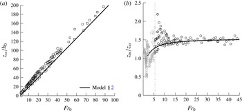
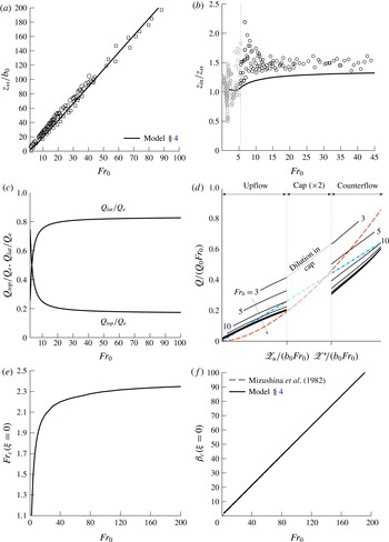
Figure 2(a) plots our theoretical solution for the steady rise height
 $z_{ss}/b_{0}$
against source Froude number
 $Fr_{0}$
. Also plotted are the measurements of Mizushina et al. (Reference Mizushina, Ogino, Takeuchi and Ikawa1982) and Burridge & Hunt (Reference Burridge and Hunt2012). Evidently, our prediction shows very good agreement with the data. Our solution reveals that
 $z_{ss}/b_{0}$
scales linearly on
 $Fr_{0}$
, following
 $z_{ss}/b_{0}=2.16Fr_{0}$
. We expect that the marginal underprediction of approximately
 $12\,\%$
compared with the previously reported
 $z_{ss}/b_{0}=2.46Fr_{0}$
(Turner Reference Turner1966; Burridge & Hunt Reference Burridge and Hunt2012) is mainly due to our simple parameterisation of the complex turbulent exchanges between the upflow and counterflow. We assumed that: (i) the entrainment coefficient
 $\unicode[STIX]{x1D6FC}_{u}$
is constant and (ii) entrainment from the upflow into the counterflow is negligible. No attempt has been made to tailor the entrainment coefficients
 $\unicode[STIX]{x1D6FC}_{u}$
and
 $\unicode[STIX]{x1D6FC}_{c}$
so as to improve agreement. Such fine-tuning, albeit useful for practical applications, is subject to somewhat arbitrary criteria and does not improve our understanding of these flows. Key statistics, such as rise height and dilution, are summarised in appendix A for different values of
 $\unicode[STIX]{x1D6FC}_{u}$
. Crucially, we show in § 4 that quantitative predictions may be improved by accounting for the confining influence that the counterflow exerts on the upflow without tailoring the entrainment coefficients.
(a) Rise height
 $z_{ss}/b_{0}$
and (b) rise height ratio
 $z_{in}/z_{ss}$
as a function of source Froude number
 $Fr_{0}$
. Our solutions (solid line) are shown with experimental data from Mizushina et al. (Reference Mizushina, Ogino, Takeuchi and Ikawa1982) (▫) and Burridge & Hunt (Reference Burridge and Hunt2012) (○). In (a), a linear best fit to the model prediction gives
 $z_{ss}/b_{0}=2.16Fr_{0}$
. In (b), the vertical line at
 $Fr_{0}=5.5$
separates highly forced releases (black) from weaker releases (grey).

Figure 2(b) plots the predicted rise height ratio
 $z_{in}/z_{ss}$
against
 $Fr_{0}$
. Our forced-fountain predictions capture well the general trend of the data from Burridge & Hunt (Reference Burridge and Hunt2012). Whilst Turner (Reference Turner1966) reported a constant rise height ratio
 $z_{in}/z_{ss}=1.43$
, Burridge & Hunt (Reference Burridge and Hunt2012) showed that this is not the case in the weak and intermediate fountain regimes
 $(Fr_{0}<3)$
. Our solution indicates that
 $z_{in}/z_{ss}$
varies rapidly with
 $Fr_{0}$
, even for forced fountains
 $(Fr_{0}>3)$
, before asymptoting to a constant value of
 $z_{in}/z_{ss}=1.52$
in the high-
 $Fr_{0}$
limit.
For
 $5<Fr_{0}<260$
, Mizushina et al. (Reference Mizushina, Ogino, Takeuchi and Ikawa1982) present measurements of the radius
 $b_{u}$
and vertical velocity
 $w_{u}$
of the upflow at different heights above a virtual point source, located a distance
 $z_{v}$
below their actual source. Consistent with their method, we determined
 $z_{v}$
by extrapolating
 $b_{u}$
to the point at which
 $b_{u}=0$
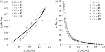
. Figures 3(a) and 3(b), respectively, plot our solutions for the radius and vertical velocity of the upflow against the vertical distance
 $\mathscr{Z}/(b_{0}Fr_{0})$
from the virtual source, where
 $\mathscr{Z}=z+z_{v}$
. By also plotting the data from Mizushina et al. (Reference Mizushina, Ogino, Takeuchi and Ikawa1982), figure 3 illustrates the good agreement between our predictions and their data. Bloomfield & Kerr (Reference Bloomfield and Kerr2000) noted that as they do not model the flow reversal region, their own predictions of
 $w_{u}$
for
 $\mathscr{Z}/(b_{0}Fr_{0})>1$
markedly diverge from the measurements of Mizushina et al. (Reference Mizushina, Ogino, Takeuchi and Ikawa1982). In contrast, our predictions of
 $w_{u}$
closely agree with the data for
 $\mathscr{Z}/(b_{0}Fr_{0})>1$
(figure 3
b), indicating that our fountain-top model is effective in capturing the bulk dynamics close to the flow reversal region.
Examining our solutions (figure 3), we find that
 $b_{u}\propto \mathscr{Z}$
and
 $w_{u}\propto 1/\mathscr{Z}$
for
 $\mathscr{Z}/(b_{0}Fr_{0})<1.5$
, i.e. the radius and vertical velocity of the upflow follow the scalings for a pure jet. This affirms our premise (§ 2) that the upflow is jet-like over the majority of its rise height (cf. Fischer et al.
Reference Fischer, List, Koh, Imberger and Brooks1979).
Upflow: (a) radius
 $b_{u}/(b_{0}Fr_{0})$
and (b) vertical velocity
 $w_{u}Fr_{0}/w_{0}$
plotted against the vertical coordinate
 $\mathscr{Z}/(b_{0}Fr_{0})$
from the virtual source. Solid lines are our predictions for the values of
 $Fr_{0}$
shown and symbols are the measurements of Mizushina et al. (Reference Mizushina, Ogino, Takeuchi and Ikawa1982).

3.1 Dynamical variability with height
The upflow Froude number
 $Fr_{u}$
at a given height provides an indication of the local fountain behaviour. Following the classification proposed by Burridge & Hunt (Reference Burridge and Hunt2012), we classify the upflow at a given height into either the highly forced
 $(Fr_{u}>5.5)$
, forced
 $(2.8<Fr_{u}\leqslant 5.5)$
, intermediate
 $(1.4<Fr_{u}\leqslant 2.8)$
or weak
 $(Fr_{u}\leqslant 1.4)$
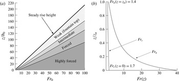
regimes. Figure 4(a) shows the regime variation with height
 $z/b_{0}$
above the source as a function of
 $Fr_{0}$
. Additionally, figure 4(b) plots the variation with height of
 $Fr_{u}$
and
 $Fr_{c}$
for
 $Fr_{0}=40$
and is illustrative of trends valid across all (sufficiently) forced fountains. It is clear from figures 4(a) and 4(b) that the upflow remains ‘forced’ (
 ${\gtrsim}3.0$
based on the existing classification) over a significant fraction of its rise height and, on rising, transitions from momentum-driven jet-like behaviour (forced regime) to buoyancy-dominated flow reversal (weak regime) over the relatively short vertical extent
 ${\sim}0.15z_{ss}$
of the intermediate regime. During this transition, the influence of the opposing buoyancy on entrainment into the upflow is strengthened. As a consequence, in practice we would anticipate strong vertical variations in
 $\unicode[STIX]{x1D6FC}_{u}$
within the intermediate regime. Contrary to the upflow, little dynamical variation is observed in the counterflow, where
 $Fr_{c}$
increases only marginally (figure 4
b). For
 $Fr_{0}>20$
, the vertical extents of each regime and the heights of the upflow
 $z_{u}$
and fountain top
 $z_{t}$
are constant fractions of the total rise height
 $z_{ss}$
:
 $$\begin{eqnarray}\frac{z_{u}}{z_{ss}}=0.76,\quad \frac{z_{t}}{z_{ss}}=0.24,\end{eqnarray}$$
or, equivalently, a rise-height to radius ratio of 4.17 (approximately).
Dynamical variability with height. (a) Local fountain behaviour versus dimensionless height. Shaded areas indicate highly forced
 $(Fr_{u}>5.5)$
, forced
 $(2.8<Fr_{u}\leqslant 5.5)$
, intermediate
 $(1.4<Fr_{u}\leqslant 2.8)$
and weak
 $(Fr_{u}\leqslant 1.4)$
regimes. (b) Variation with height of
 $Fr_{u}$
and
 $Fr_{c}$
in a high-
 $Fr_{0}$
fountain for
 $Fr_{0}=40$
. When suitably scaled, near-identical curves of
 $Fr_{u}$
and
 $Fr_{c}$
are obtained for
 $Fr_{0}>40$
, so that the trends in (b) are representative of all sufficiently forced releases.

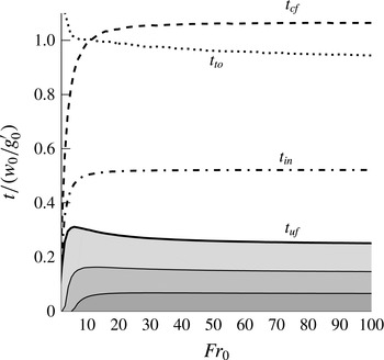
Consistent with the invariance of the vertical extents of each region (3.1) (and with the vertical velocities, figure 3) is the invariance of travelling times through a suitably forced fountain. The time taken for a fluid parcel to rise through the upflow,
 $t_{uf}$
, and to fall through the counterflow,
 $t_{cf}$
, can be calculated as
 $$\begin{eqnarray}t_{uf}=\int _{0}^{z_{u}}\frac{1}{w_{u}}\,\text{d}z,\quad t_{cf}=\int _{0}^{z_{u}^{\ast }}\frac{1}{w_{c}}\,\text{d}z^{\ast }.\end{eqnarray}$$
Figure 5 plots
 $t_{uf}$
and
 $t_{cf}$
, normalised by the buoyancy time-scale
 $w_{0}/g_{0}^{\prime }$
, against the source Froude number. The shaded regions beneath the curve showing
 $t=t_{uf}$
indicate the time taken to travel through each regime (cf. figure 4
a). Also plotted are the times to attain the initial rise height
 $t_{in}$
, calculated from (3.2a
) at the first iteration, and the estimated turnover time in the cap region
 $t_{to}$
(see § 3.3). The local maximum in
 $t_{uf}$
reached for
 $Fr_{0}\approx 6$
disappears shortly after the formation of the highly forced section of the flow. For high
 $Fr_{0}$
, the travel time through each regime constitutes a constant proportion of the total travel time, as can be clearly seen in the plot. For the upflow, despite being of a relatively limited vertical extent, it is the rise through the intermediate regime that takes the longest. Based on our predictions, the ratio
 $t_{uf}/t_{cf}$
asymptotes to:
 $$\begin{eqnarray}\frac{t_{uf}}{t_{cf}}=0.24,\end{eqnarray}$$
in other words the time taken to rise through the upflow is roughly a factor of four less than the time to descend in the counterflow. For chemically reacting flows, knowledge of the residence time of a volume of fluid is crucial in order to determine evolving contaminant concentrations. Although we do not include any chemistry in our model, and as such the ratio (3.3) is only strictly valid for an inert contaminant, we anticipate similar findings to hold in reacting fountains. Thus, figure 5 highlights the necessity to accurately model every section of a fountain.
Variation with
 $Fr_{0}$
of travelling times through the body of the fountain normalised by the buoyancy time-scale
 $w_{0}/g_{0}^{\prime }$
. Shaded areas under each (solid) curve indicate the contribution to rise time in the upflow from the different regimes (cf. figure 4
a). Reading top-to-bottom the curves show: the time for fluid to descend in the counterflow
 $t_{cf}$
, the turnover time in the fountain top
 $t_{to}$
, the time taken to reach the initial rise height
 $t_{in}$
and the time fluid spends rising through the upflow
 $t_{uf}$
.

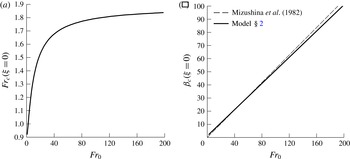
The counterflow Froude number
 $Fr_{c}(\unicode[STIX]{x1D709}=0)$
at the level of the source
 $\unicode[STIX]{x1D709}=0$
describes the relative magnitudes of the fluxes of volume, momentum and buoyancy within the outflow from the fountain. By analogy with a plume, we note that the outflow becomes increasingly forced as
 $Fr_{0}$
increases and in accord with the scalings deduced by Burridge & Hunt (Reference Burridge and Hunt2014), we find that
 $Fr_{c}(\unicode[STIX]{x1D709}=0)$
asymptotes to a constant value in the high-
 $Fr_{0}$
limit, as indicated in figure 6(a). Thus, in this limit, the counterflow evolves towards an asymptotic balance between inertial and gravitational forces at the level of the outflow, irrespective of the source conditions. Finally, in line with the experiments of Mizushina et al. (Reference Mizushina, Ogino, Takeuchi and Ikawa1982) and scaling arguments of Burridge & Hunt (Reference Burridge and Hunt2014), we predict that the outflow radius
 $\unicode[STIX]{x1D6FD}_{c}(\unicode[STIX]{x1D709}=0)$
scales linearly on
 $Fr_{0}$
(figure 6
b).
Outflow: (a) Froude number
 $Fr_{c}(\unicode[STIX]{x1D709}=0)$
against
 $Fr_{0}$
and (b) radius
 $\unicode[STIX]{x1D6FD}_{c}(\unicode[STIX]{x1D709}=0)$
(solid line) with best fit by Mizushina et al. (Reference Mizushina, Ogino, Takeuchi and Ikawa1982) (dashed line).

3.2 Dilution rates in fountains
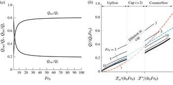
The result (3.3) is complemented by the result that at high
 $Fr_{0}$
the fountain-top
 $(Q_{top})$
and lateral
 $(Q_{lat})$
entrainment fluxes asymptote to constant fractions of the total volume flux
 $Q_{e}$
 $(=Q_{lat}+Q_{top})$
of ambient fluid entrained into the fountain (figure 7
a):
 $$\begin{eqnarray}\frac{Q_{lat}}{Q_{e}}=0.81,\quad \frac{Q_{top}}{Q_{e}}=0.19.\end{eqnarray}$$
Rates of dilution in a fountain,
 $Q(\mathscr{Z})/Q_{0}$
, are a quantity of practical interest to environmentalists, owing, for example, to concerns regarding waste water discharges into the oceans (Koh & Brooks Reference Koh and Brooks1975). These dilution rates are plotted in figure 7(b). Also plotted are the dilution rates for a turbulent pure jet and a turbulent pure plume as inferred from Fischer et al. (Reference Fischer, List, Koh, Imberger and Brooks1979, pages 328 and 332), namely
 $$\begin{eqnarray}\frac{Q}{Q_{0}Fr_{0}}=0.143\frac{\mathscr{Z}}{b_{0}Fr_{0}},\quad \frac{Q}{Q_{0}Fr_{0}}=0.070\left(\frac{\mathscr{Z}}{b_{0}Fr_{0}}\right)^{5/3},\end{eqnarray}$$
where we recall that
 $\mathscr{Z}=z+z_{v}$
. To enable direct comparison between fountains, jets and plumes, the abscissa in figure 7(b) represents the total distance from the source in the direction of flow. Dilution within the cap region is not shown, given that we have made no claim regarding the time-averaged velocity profile within it. The separation between the two vertical lines shown is twice the vertical extent of the fountain cap (
 $2z_{t}$
); the value of dilution at the top of the upflow is that coincident with the first vertical line and dilution at the top of the counterflow is that coincident with the second. The vertical step at the breaks in each line of dilution corresponds to the dilution that occurs in the cap itself. Note that it is not possible to add scales to the horizontal axis on figure 7(b) (and likewise for figure 9), because in the upflow, the scale is shifted by a different amount (
 $z_{v}$
) for each
 $Fr_{0}$
; the curves have only one point in common, which is marked by
 $\mathscr{Z}_{u}$
, i.e. the location at which the flow starts to reverse.
(a) Entrainment flux ratios
 $Q_{top}/Q_{e}$
and
 $Q_{lat}/Q_{e}$
as a function of
 $Fr_{0}$
, where the total entrainment flux
 $Q_{e}=Q_{lat}+Q_{top}$
. (b) Local dilution ratio in a fountain
 $Q/(Q_{0}Fr_{0})$
for
 $Fr_{0}=\{3,5,10,20,40,60,80,100\}$
(solid lines) against normalised distance from source in the direction of flow, together with dilution rates for a pure plume (red dashed line) and for a pure jet (blue dash-dotted line). The vertical axis of the fountain has been ‘unfolded’ to combine upflow, flow reversal and counterflow onto one axis. The arrow points in the direction of increasing
 $Fr_{0}$
.

It is immediately apparent that neglecting entrainment through the cap leads to a gross underestimation of the total counterflowing volume flux (and thus of dilution) in moderate-
 $Fr_{0}$
fountains. For high-
 $Fr_{0}$
fountains, the diluting behaviour closely follows that of a jet,
 $Q\propto \mathscr{Z}$
. Perhaps surprisingly, this is also the case for the counterflow, where we might have expected a closer similarity with dilution in a plume. Overall, the dilution rates with the ambient are less than for a jet that develops over a similar distance. Our solutions predict that at the level of the outflow
 $Q_{out}=0.48Q_{0}Fr_{0}$
, somewhat lower than
 $Q_{out}=0.71Q_{0}Fr_{0}$
measured by Burridge & Hunt (Reference Burridge and Hunt2016). The mismatch in outflow volume fluxes can in part be explained by the lower predicted rise height: by rising 12 % less high, our model for a forced fountain entrains less ambient fluid laterally. In § 4, we show that a closer estimate of dilution may be recovered without tailoring entrainment coefficients.
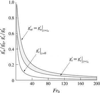
Finally, we inspect the buoyancies attained at the peak of a fountain and at the level of its outflow. An estimate of the reduced gravity within the fountain top
 $g_{top}^{\prime }$
can be gained from figure 8, where we plot the reduced gravities of fluid entering (
 $g_{u}^{\prime }(z=z_{u})=g_{ut}^{\prime }$
) and leaving (
 $g_{c}^{\prime }(z=z_{u})=g_{t}^{\prime }$
) the fountain top against
 $Fr_{0}$
. Evidently,
 $g_{t}^{\prime }\leqslant g_{top}^{\prime }\leqslant g_{ut}^{\prime }$
, thus
 $g_{top}^{\prime }$
must lie within the shaded region in figure 8. Also plotted are our predictions for reduced gravity at the level of the outflow,
 $g_{c}^{\prime }(z=0)$
. For high-
 $Fr_{0}$
, the reduced gravities approach
 $$\begin{eqnarray}\frac{g_{ut}^{\prime }}{g_{0}^{\prime }Fr_{0}}=9.06,\quad \frac{g_{t}^{\prime }}{g_{0}^{\prime }Fr_{0}}=5.94,\quad \frac{g_{c}^{\prime }(z=0)}{g_{0}^{\prime }Fr_{0}}=2.05.\end{eqnarray}$$
Whilst
 $g_{c}^{\prime }(z=0)$
asymptotes rapidly,
 $g_{ut}^{\prime }$
and
 $g_{t}^{\prime }$
keep evolving (albeit weakly) past
 $Fr_{0}=200$
, hence we do not count them amongst the invariants (§ 3.4). Note that
 $g_{ut}^{\prime }$
and
 $g_{t}^{\prime }$
differ by 34 % for
 $E_{top}=0.525$
, emphasising again the necessity to account for fountain-top entrainment.
Reduced gravities of fluid entering the fountain top from the upflow (
 $g_{ut}^{\prime }$
), of fluid leaving the fountain top as the counterflow (
 $g_{t}^{\prime }$
) and of fluid at the outflow level (
 $g_{c}^{\prime }(z=0)$
) plotted against
 $Fr_{0}$
. For a given
 $Fr_{0}$
, the shaded region provides an estimate of the reduced gravity in the region of flow reversal
 $g_{top}^{\prime }$
. In the high-
 $Fr_{0}$
limit, the reduced gravities approach
 $g_{ut}^{\prime }/g_{0}^{\prime }=9.06/Fr_{0}$
,
 $g_{t}^{\prime }/g_{0}^{\prime }=5.94/Fr_{0}$
and
 $g_{c}^{\prime }(z=0)/g_{0}^{\prime }=2.05/Fr_{0}$
.

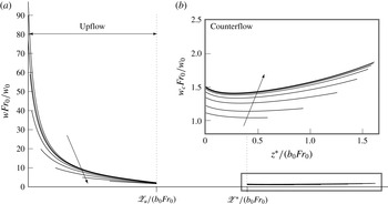
(a) Evolution of the vertical velocity in the upflow and counterflow for
 $Fr_{0}=\{3,5,10,20,40,60,80,100\}$
, with the abscissa as in figure 7(b). The inset (b) shows a zoomed view of the counterflow region outlined. The arrows point in the direction of increasing
 $Fr_{0}$
.

3.3 Turnover time in the cap
In its instantaneous nature, the fountain top consists of periodic lobes or eddies that form and subsequently spill onto the sides of the fountain. In forced fountains, Burridge & Hunt (Reference Burridge and Hunt2013) have suggested that the dominant fluctuations are caused by eddies cyclically building up at the largest scale (
 ${\sim}b_{ut}$
) and collapsing. They measured a near constant period of oscillation of
 $T_{p}/(w_{0}/g_{0}^{\prime })=2$
, consistent with the observations of Pantzlaff & Lueptow (Reference Pantzlaff and Lueptow1999) who report
 $T_{p}/(w_{0}/g_{0}^{\prime })=1{-}2$
.
By definition, our time-averaged model of the cap cannot capture the details of the highly unsteady fluctuations at the fountain top (see Debugne & Hunt (Reference Debugne and Hunt2016) for an extended discussion on the merits and drawbacks of applying a time-averaged formulation to the fountain top). Nevertheless, the model should be able to inform us about the mean turnover time,
 $t_{to}$
(the subscript ‘to’ indicating ‘turnover’), i.e. the time taken by the flow to reverse at the fountain top. In turn,
 $t_{to}$
must be related to the dominant fluctuations studied by Burridge & Hunt (Reference Burridge and Hunt2013). Therefore, we expect
 $t_{to}\sim w_{0}/g_{0}^{\prime }$
.
Without the evolution of the time-averaged velocity in the cap,
 $t_{to}$
cannot be calculated directly. However, we can gain some insight regarding the magnitude of
 $t_{to}$
by conducting a volume balance throughout the fountain. Over some time interval
 $\unicode[STIX]{x0394}T$
, the total volume of fluid in the fountain,
 $V=\unicode[STIX]{x03C0}b_{t}^{2}z_{u}+2\unicode[STIX]{x03C0}b_{t}^{3}/3$
, is comprised of fluid dispensed at the source,
 $Q_{0}\unicode[STIX]{x0394}T$
, and of fluid entrained from the ambient,
 $Q_{e}\unicode[STIX]{x0394}T$
. Taking
 $\unicode[STIX]{x0394}T$
as the total travel time of a fluid particle through the fountain,
 $\unicode[STIX]{x0394}T=t_{uf}+t_{to}+t_{cf}$
, enables us to separate the contributions to
 $Q_{e}$
from entrainment through the top and entrainment through the sides. The volume balance can be expressed as
 $$\begin{eqnarray}V=\unicode[STIX]{x0394}T(Q_{0}+Q_{e})=(t_{uf}+t_{to}+t_{cf})Q_{0}+t_{to}Q_{top}+t_{cf}Q_{lat},\end{eqnarray}$$
giving the following estimate for the turnover time
 $$\begin{eqnarray}t_{to}=\frac{(V/Q_{0})-t_{uf}-t_{cf}(1+Q_{lat}/Q_{0})}{1+Q_{top}/Q_{0}}.\end{eqnarray}$$
The turnover time
 $t_{to}$
calculated from (3.8) is plotted on figure 5 as a dotted line. It is evident that for high Froude numbers,
 $t_{to}$
is indeed of the order of
 $w_{0}/g_{0}^{\prime }$
. We therefore conclude that the present modelling approach is successful in capturing the bulk dynamics of the fountain top.
3.4 Asymptotic structure of forced fountains
Our previous findings, specifically the constant apportionment of the upflow (figure 4
a) and the invariance of the ratios (3.1), (3.3) and (3.4), reveal that, suitably scaled, the bulk structure of a fountain is unchanging for sufficiently forced releases. In other words, in the limit of high-
 $Fr_{0}$
there is a self-preserving development of the bulk characteristics and organisation of a fountain. While there is a strong dynamical variability with height (notably the local Froude numbers are not invariant, figure 4
b) and as such even in a high-
 $Fr_{0}$
limit the fountain cannot be truly self-similar, we may regard the bulk flow as globally self-similar. Global similarity must be contrasted with local similarity, the latter referring to the invariance of the radial profiles of local flow variables. There is no general consensus regarding the level of (local) self-similarity, if any, that is reached in fountains; we return to this issue in light of our solutions in § 5.
Clearly, the radial variation of vertical velocity, as measured by experimentalists, may not be extracted from our simulations, where, in the top-hat formalism used,
 $w_{u}$
and
 $w_{c}$
represent cross-stream-averaged vertical velocities. Nevertheless, top-hat variables are indicative of the magnitude of these profiles and are useful for informing us about the relevant scalings. Thus, to shed further light on the internal structure of a forced fountain, in figure 9 we plot the evolution of the velocities
 $w_{u}$
and
 $w_{c}$
against downstream distance from the (virtual) source.
In the upflow, following a near-field jet-like development phase (whose extent depends on the forcing provided at the source), the velocities approximately collapse as they approach the level of the fountain top. As the influence of the source momentum flux of the release decreases farther away from the source, it is primarily the local competition between inertia and buoyancy, encompassed in
 $Fr_{u}$
, which determines the subsequent development of the flow. The dependence on
 $Fr_{u}(z)$
, rather than
 $Fr_{0}$
, thus motivates the approximate collapse in figure 9(a). Likewise, in the counterflow, where
 $Fr_{c}$
varies weakly (figure 4
b), there is close similitude between the velocity curves. The initial dip in
 $w_{c}$
, occurring around
 $z^{\ast }/(b_{0}Fr_{0})=0.25$
(equivalent to
 $\mathscr{Z}/(b_{0}Fr_{0})=1.5$
in the upflow coordinates), coincides with the rapid radial growth of the upflow (figure 3): as the upflow radius
 $b_{u}$
decreases with increasing
 $z^{\ast }$
, the counterflow area
 $\unicode[STIX]{x03C0}(b_{c}^{2}-b_{u}^{2})$
expands, prompting the counterflow to decelerate to satisfy continuity. This effect, which is likely a consequence of posing
 $b_{c}=\text{const.}$
, can be mitigated by allowing for greater entrainment into the counterflow. In the absence of detailed measurements of
 $w_{c}$
(or, indeed,
 $\unicode[STIX]{x1D6FC}_{c}$
) however, such fine-tuning finds no clear justification.
4 An alternative body force formulation
The discussion on different body force formulations was purposefully delayed until now so as to not distract the reader by having to compare several modelling assumptions at once. As it stands, the current model provides insights into the local and bulk properties of a forced fountain. However, since the precise interaction between the upflow and the counterflow is in debate, it is opportune to explore alternative formulations of that interaction. In this section, we recast the equations for the conservation of momentum under different assumptions and highlight the main differences between the resulting predictions for both body-force formulations considered. In doing so, we show that the three-region model is robust, complying well with modifications to its governing equations.
In his paper, McDougall (Reference Mcdougall1981) proposed two different formulations for the body forces acting on a fountain (see also Bloomfield & Kerr Reference Bloomfield and Kerr2000). Hereinafter, we refer to the two formulations as F1 and F2.
In the first formulation, F1, it is assumed that the pressure is hydrostatic everywhere across the fountain. F1 leads to (2.13)–(2.14) and (2.22)–(2.23) upon invoking that the outflow radius is constant with height. In fact, F1 directly follows from the traditional theory of coaxial plumes after Morton (Reference Morton1962).
For the second formulation, F2, McDougall (Reference Mcdougall1981) argued that, in the established fountain, the shrouding counterflow effectively confines the upflow and acts as the ‘ambient’ or external environment to the fountain core. In this picture, the upflow experiences a buoyant acceleration relative to that of the counterflow, which modifies the governing equations. The derivation, omitted here for concision, is presented in detail in appendix C.

Figure 10 reproduces some of the previous results and allows comparison between both body force formulations. Overall, the agreement with the experimental data improves from F1 to F2, with the fountain outline being particularly well estimated (figures 10
a and 10
f). Under F2 the fountain rises higher in the steady state to reach
 $z_{ss}/b_{0}=2.36Fr_{0}$
, close to the accepted rise height of
 $2.46Fr_{0}$
(as reviewed in Hunt & Burridge (Reference Hunt and Burridge2015)). It is of note that this increase in rise height stems principally from the narrowing of the upflow. This is apparent on comparing the rates of spread
 $\text{d}\unicode[STIX]{x1D6FD}_{u}/\text{d}\unicode[STIX]{x1D709}$
under F1, (2.13a
), and under F2, (C 5); since the gravitational acceleration in the counterflow (first term in
 $R_{1}$
) exceeds the relative acceleration of the frame of reference (second term in
 $R_{1}$
, see (C 7)), we find that
 $R_{1}<0$
at all heights so that
 $(\text{d}\unicode[STIX]{x1D6FD}_{u}/\text{d}\unicode[STIX]{x1D709})_{F2}<(\text{d}\unicode[STIX]{x1D6FD}_{u}/\text{d}\unicode[STIX]{x1D709})_{F1}$
. Thus the relative acceleration framework restricts the growth of the upflow, manifesting the confining influence of the counterflow.
In the high-
 $Fr_{0}$
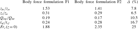
limit, all herein reported ratios again preserve their invariance but asymptote to slightly different values, as summarised in table 1. Notably, dilution rates in the counterflow increase to
 $Q_{out}=0.60Q_{0}Fr_{0}$
(compare figures 7
b and 10
d) and markedly exceed those of a jet (figure 10
d). This increase in dilution with F2, leading to lower values of
 $g_{c}^{\prime }$
, also gives rise to increased forcing in the outflow, signified by
 $Fr_{c}(z=0)=2.35$
at the level of the source.
Asymptotic values of key ratios and their percentage difference for high-
 $Fr_{0}$
‘forced’ fountains for body force formulations F1 and F2.

Deciding which of the two body force formulations provides a more lifelike description of a forced fountain can have far-reaching consequences in industrial applications, given, for instance, that the dilution at the level of the outflow varies as much as 25 % between formulations. Experimental evidence would suggest that McDougall’s second approach is possibly more accurate. Both formulations generally lie in close quantitative and qualitative agreement and a definite verdict lies beyond the scope of this paper. Reassuringly, it has been shown that the utility of the three-region model is not restricted to a specific set of governing equations, but that it can successfully accommodate new modelling hypotheses.
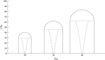
Envelopes for a turbulent forced fountain formed at source Froude numbers
 $Fr_{0}=\{20,30,40\}$
predicted by our three-region model (§ 2). The radial scale (not shown) is identical to the vertical scale. The external envelope (solid line) and internal envelopes (dashed lines) highlight the three regions.

5 Conclusions
We have presented a three-region theoretical model describing the upflow, counterflow and fountain top of a quasi-steady turbulent axisymmetric forced fountain. In assigning the fountain a finite region at its top where the flow is allowed to reverse and to entrain ambient fluid, we not only replicate a phenomenon that is observed in practice, but we also eliminate the deviations near the fountain top that burden previous models. Crucially, the three-region model enables one to predict the physical outline of a fully turbulent forced fountain, as is illustrated in figure 11. Predictions of the rise height, upflow radius and upflow vertical velocity are in close agreement with existing experimental data. Moreover, solutions for the fluxes within the fountain are in accord with the scalings deduced by Burridge & Hunt (Reference Burridge and Hunt2014), thus further supporting the appropriateness of our model. Significantly, at large source Froude numbers
 $(Fr_{0})$
, we predict that five key ratios approach constant values, namely the ratios of:
-
(1) initial and steady-state rise heights,
 $z_{in}/z_{ss}=1.53\;(1.41)$
;
-
(2) vertical extents of the fountain top and upflow,
$z_{t}/z_{u}=0.31\;(0.29)$
; -
(3) fluxes entrained into the fountain top and laterally into the counterflow,
$Q_{top}/Q_{lat}=0.19\;(0.17)$
; -
(4) travelling times through the upflow and through the counterflow,
$t_{uf}/t_{cf}=0.24\;(0.28)$
; and -
(5) forces of inertia and buoyancy acting on the counterflow at the level of the source,
$Fr_{c}(z=0)=1.88\;(2.35)$
.





(In parentheses are the values of these ratios for the body force formulation F2.) These ratios, whose invariance is attributed to large-
 $Fr_{0}$
flows, describe intrinsic features of fountains: specifically, the finite vertical extent of the flow, entrainment of ambient fluid and the competition between inertial and buoyancy forces. We therefore suggest that a continuous negatively buoyant localised release gives rise to a ‘forced’ fountain when the five key ratios (1)–(5) are invariant. In this high-
 $Fr_{0}$
limit, the forced fountain may then be regarded as exhibiting ‘globally’ self-preserving behaviour with respect to
 $Fr_{0}$
. In light of the findings reported herein, this limit seems to be attained for
 $Fr_{0}\gtrsim 20$
. Although this is significantly higher than the threshold of
 $Fr_{0}\gtrsim 5.5$
previously suggested by Burridge & Hunt (Reference Burridge and Hunt2012), their limit is based on the occurrence of vortex pinch-off during the fountain start-up and does not inform us about the state of self-preservation within the established fountain. Our classification not only indicates the source conditions required to produce a forced fountain, it also provides a means for experimentalists to discern between the upflowing core and fountain top. Future insights into the turbulent exchanges between upflow and counterflow can readily be implemented in our model by modifying the interaction terms (2.15).
One thorny question that remains open is the degree to which inner flow variables can be considered, if at all, self-similar. Neither the measurements of Mizushina et al. (Reference Mizushina, Ogino, Takeuchi and Ikawa1982) nor those of Cresswell & Szczepura (Reference Cresswell and Szczepura1993) provide conclusive evidence. In their direct simulation of a forced fountain at
 $Fr_{0}=7$
, Williamson et al. (Reference Williamson, Armfield and Lin2011) noted that the flow variables in the counterflow reached some degree of self-preservation just beneath the cap. They argued that the relative disconnectedness between turbulent structures in the counterflow and in the upflow allowed the counterflow to develop approximately as a self-similar annular plume. It is not clear why the same line of reasoning should not apply to the upflow. In Williamson et al.’s simulation, the relatively limited extent of the upflow (the potential core merges only
 $4b_{0}{-}5b_{0}$
before the onset of flow reversal) indeed precludes the possibility of developing self-preserving behaviour.
In the absence of detailed measurements of the internal variables for high-
 $Fr_{0}$
fountains, questions regarding the nature of turbulent exchanges or the self-similarity of the flow cannot be alleviated. It therefore seems inevitable that any major improvement in the understanding and in the modelling of forced fountains should stem from a dedicated experimental campaign (or, indeed, from numerical advances).
Acknowledgements
G.R.H. and A.L.R.D. wish to thank Dr A. B. Shrinivas for his contribution to an early draft of this manuscript. The authors also gratefully acknowledge funding from the Qualcomm European Research Studentships in Technology and from the UK Engineering and Physical Sciences Research Council (EPSRC grant number EP/L504920/1).
Appendix A. Sensitivity to modelling assumptions
A.1 Constant entrainment coefficients
When presenting a model for forced fountains, it has almost become paradigm to vary the entrainment coefficients
 $\unicode[STIX]{x1D6FC}_{u}$
and
 $\unicode[STIX]{x1D6FC}_{c}$
until a given statistic (typically, the quasi-steady rise height) matches the values reported in experiments. Often, this statistic is arbitrarily defined and alone cannot be a measure of the prowess of the model.
There is overwhelming evidence that the entrainment coefficient should not be treated as a constant in jets and plumes (e.g. Ezzamel, Salizzoni & Hunt Reference Ezzamel, Salizzoni and Hunt2015; van Reeuwijk & Craske Reference van Reeuwijk and Craske2015), though its exact dependence on the local conditions is unknown. To date, there has not been a study dedicated to the variation of
 $\unicode[STIX]{x1D6FC}$
in fountains, where the flow transitions from forced, to pure, to lazy. Given that our primary aim was to develop a robust model for forced fountains, in light of these uncertainties there seemed to be limited scientific value in recommending one single figure above another for the entrainment coefficient in fountains.
For practical applications however, it might be useful to provide one globally representative value for entrainment in fountains. Some key variables were calculated for different
 $\unicode[STIX]{x1D6FC}_{u}$
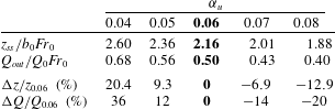
in table 2 (keeping all other parameters fixed). As expected, a decrease in
 $\unicode[STIX]{x1D6FC}_{u}$
(implying that less momentum is lost to mixing with the counterflow) leads to a (nonlinear) increase in predicted rise heights. The effects of varying
 $\unicode[STIX]{x1D6FC}_{u}$
on
 $Q_{out}$
are exacerbated because they are twofold: for lower
 $\unicode[STIX]{x1D6FC}_{u}$
, (i) travelling a greater vertical distance allows the counterflow to dilute further, and (ii) less counterflow fluid is re-entrained into the upflow. Thus, to the engineer interested solely in estimating rise heights or dilutions, table 2 suggests that a fixed coefficient between
 $\unicode[STIX]{x1D6FC}_{u}\approx 0.4{-}0.5$
would provide a better fit to experimental data.
Predictions for the normalised steady-state rise height
 $z_{ss}/b_{0}Fr_{0}$
and dilution at the outflow level
 $Q_{out}/Q_{0}Fr_{0}$
for different values of
 $\unicode[STIX]{x1D6FC}_{u}$
with their percentage difference from the base case (§ 2), highlighted in bold.

A.2 Counterflow conservation equations for
$b_{c}\neq \text{const.}$

As demonstrated in § 2.3, the assumption of constant counterflow radius
 $b_{c}=\text{const.}$
considerably simplifies the numerical implementation of the counterflow by reducing it to a single differential equation (2.22). However, this simplification is not a requirement of the three-region model, and we may readily derive the equations for the full formulation of the counterflow without assuming
 $b_{c}=\text{const.}$
Starting from the non-dimensional equations for conservation of the fluxes of volume, momentum and buoyancy in the counterflow,
 $$\begin{eqnarray}\frac{\text{d}q_{c}}{\text{d}\unicode[STIX]{x1D709}^{\ast }}=\frac{5}{3}\frac{\unicode[STIX]{x1D6FC}_{c}}{\unicode[STIX]{x1D6FC}_{u}}\unicode[STIX]{x1D6FD}_{c}\unicode[STIX]{x1D714}_{c}-\frac{5}{3}\unicode[STIX]{x1D6FD}_{u}\unicode[STIX]{x1D714}_{u},\quad \frac{\text{d}m_{c}}{\text{d}\unicode[STIX]{x1D709}^{\ast }}=\frac{5}{6}(\unicode[STIX]{x1D6FD}_{c}^{2}-\unicode[STIX]{x1D6FD}_{u}^{2})^{1/2}\frac{\unicode[STIX]{x1D714}_{c}^{2}}{\unicode[STIX]{x1D6FC}_{u}Fr_{c}^{2}}-\frac{5}{3}\unicode[STIX]{x1D6FD}_{c}\unicode[STIX]{x1D714}_{u}\unicode[STIX]{x1D714}_{c}\end{eqnarray}$$
and
 $$\begin{eqnarray}\frac{\text{d}f_{c}}{\text{d}\unicode[STIX]{x1D709}^{\ast }}=-\frac{5}{3}\frac{\unicode[STIX]{x1D6FD}_{u}\unicode[STIX]{x1D714}_{u}\unicode[STIX]{x1D714}_{c}^{2}}{(\unicode[STIX]{x1D6FD}_{c}^{2}-\unicode[STIX]{x1D6FD}_{u}^{2})^{1/2}Fr_{c}^{2}},\end{eqnarray}$$
respectively, we rearrange (A 1)–(A 2) in terms of local variables. After some manipulation, this yields
 $$\begin{eqnarray}\displaystyle & \displaystyle \frac{\text{d}\unicode[STIX]{x1D6FD}_{c}}{\text{d}\unicode[STIX]{x1D709}^{\ast }}=\frac{5}{3}\left(\frac{\unicode[STIX]{x1D6FC}_{c}}{\unicode[STIX]{x1D6FC}_{u}}-\frac{\unicode[STIX]{x1D6FD}_{u}}{\unicode[STIX]{x1D6FD}_{c}}\right)-\frac{5}{6}\frac{\unicode[STIX]{x1D6FD}_{u}}{\unicode[STIX]{x1D6FD}_{c}}\left(\frac{\unicode[STIX]{x1D714}_{u}}{\unicode[STIX]{x1D714}_{c}}+\frac{\unicode[STIX]{x1D714}_{c}}{\unicode[STIX]{x1D714}_{u}}\right)-\frac{5}{12\unicode[STIX]{x1D6FC}_{u}}\frac{1}{\unicode[STIX]{x1D6FD}_{c}}\left(\frac{\unicode[STIX]{x1D6FD}_{a}}{Fr_{c}^{2}}+\frac{\unicode[STIX]{x1D6FD}_{u}}{Fr_{u}^{2}}\right), & \displaystyle\end{eqnarray}$$
 $$\begin{eqnarray}\displaystyle & \displaystyle \frac{\text{d}\unicode[STIX]{x1D714}_{c}}{\text{d}\unicode[STIX]{x1D709}^{\ast }}=\frac{5}{3}\frac{\unicode[STIX]{x1D714}_{c}}{\unicode[STIX]{x1D6FD}_{a}}\left(\frac{1}{2\unicode[STIX]{x1D6FC}_{u}}\frac{1}{Fr_{c}^{2}}-\frac{\unicode[STIX]{x1D6FC}_{c}}{\unicode[STIX]{x1D6FC}_{u}}\frac{\unicode[STIX]{x1D6FD}_{c}}{\unicode[STIX]{x1D6FD}_{a}}\right) & \displaystyle\end{eqnarray}$$
and
 $$\begin{eqnarray}\frac{\text{d}Fr_{c}}{\text{d}\unicode[STIX]{x1D709}^{\ast }}=\frac{5}{3}\frac{Fr_{c}}{\unicode[STIX]{x1D6FD}_{a}}\left(\frac{1}{4}\frac{\unicode[STIX]{x1D6FD}_{u}}{\unicode[STIX]{x1D6FD}_{a}}\frac{\unicode[STIX]{x1D714}_{u}}{\unicode[STIX]{x1D714}_{c}}+\frac{5}{8\unicode[STIX]{x1D6FC}_{u}}\frac{1}{Fr_{c}^{2}}-\frac{\unicode[STIX]{x1D6FC}_{c}}{\unicode[STIX]{x1D6FC}_{u}}\frac{\unicode[STIX]{x1D6FD}_{c}}{\unicode[STIX]{x1D6FD}_{a}}\right),\end{eqnarray}$$
with
 $\unicode[STIX]{x1D6FD}_{a}=(\unicode[STIX]{x1D6FD}_{c}^{2}-\unicode[STIX]{x1D6FD}_{u}^{2})^{1/2}$
and initial conditions given by (2.18) and (2.20). The solution procedure (§ 2.4) remains unchanged.
For the same entrainment values as used in § 2, under this formulation we predict a steady-state rise height of
 $z_{ss}=2.02b_{0}Fr_{0}$
, i.e. approximately a 6 % decrease from our previous estimate (figure 2
a). Consistent with the approximation adopted in § 2, we observe that the counterflow radius
 $\unicode[STIX]{x1D6FD}_{c}$
exhibits little variation over the rise height (figure 12); specifically,
 $\unicode[STIX]{x1D6FD}_{c}$
is found to range from
 $\unicode[STIX]{x1D6FD}_{c}(\mathscr{Z}^{\ast }=0)=0.51Fr_{0}$
at the fountain top to
 $\unicode[STIX]{x1D6FD}_{c}(\mathscr{Z}^{\ast }=\mathscr{Z}_{u}^{\ast })=0.49Fr_{0}$
at the level of the outflow, with a weak minimum around mid-height (i.e. at
 $\mathscr{Z}^{\ast }\approx 2\mathscr{Z}_{u}^{\ast }/3$
). It is presumably the narrowing of the counterflow that is responsible for the decrease in predicted rise height. Such a narrowing of the fountain envelope has not been reported before and appears unphysical. Importantly, overall the predicted values of
 $\unicode[STIX]{x1D6FD}_{c}(\mathscr{Z})$
lie close to the constant counterflow radius
 $\unicode[STIX]{x1D6FD}_{c}=0.50Fr_{0}$
predicted by our simplified model and therefore support its use.
Variation in height of the non-dimensional counterflow radius
 $\unicode[STIX]{x1D6FD}_{c}$
under the formulation (A 3)–(A 5) for
 $Fr_{0}=\{5,10,20,40,60,80,100\}$
(continuous lines) together with our prediction (§ 2, figure 6
b) under the simplification
 $\unicode[STIX]{x1D6FD}_{c}=\text{const.}$
(dashed line). The arrow indicates the direction of increasing
 $Fr_{0}$
. Despite some slight variation,
 $\unicode[STIX]{x1D6FD}_{c}(\mathscr{Z}^{\ast })$
remains close to the constant radius
 $\unicode[STIX]{x1D6FD}_{c}=0.50Fr_{0}$
predicted by our simplified model.

Appendix B. Plume conservation equations
For a plume rising through a quiescent and uniform environment, conservation of the fluxes of volume, vertical momentum and buoyancy requires, respectively
 $$\begin{eqnarray}\frac{\text{d}Q}{\text{d}z}=2\unicode[STIX]{x03C0}b(\unicode[STIX]{x1D6FC}w),\quad \frac{\text{d}M}{\text{d}z}=\unicode[STIX]{x03C0}b^{2}g^{\prime },\quad \frac{\text{d}B}{\text{d}z}=0\end{eqnarray}$$
(e.g. Hunt & Kaye Reference Hunt and Kaye2005). By comparison with the conservation equations in fountains given by (2.3) and (2.6), we notice that in a plume: (i) buoyancy accelerates the flow, and (ii) in the absence of a counterflow, there is no redistribution of momentum or buoyancy across the flow. In terms of the dimensionless quantities introduced in (2.7) and (2.9), (B 1) can be rewritten as
 $$\begin{eqnarray}\frac{\text{d}q}{\text{d}\unicode[STIX]{x1D709}}=\frac{5}{3}\unicode[STIX]{x1D6FD}\unicode[STIX]{x1D714},\quad \frac{\text{d}m}{\text{d}\unicode[STIX]{x1D709}}=\frac{5}{6\unicode[STIX]{x1D6FC}}\frac{\unicode[STIX]{x1D6FD}\unicode[STIX]{x1D714}^{2}}{Fr^{2}},\quad \frac{\text{d}f}{\text{d}\unicode[STIX]{x1D709}}=0\end{eqnarray}$$
(cf. the corresponding relations for a fountain in (2.10)). Substituting (2.11) and (2.12), which remain unchanged for the plume, into (B 2) leads to
 $$\begin{eqnarray}\frac{\text{d}\unicode[STIX]{x1D6FD}}{\text{d}\unicode[STIX]{x1D709}}=\frac{5}{3}\left(1-\frac{1}{4\unicode[STIX]{x1D6FC}}\frac{1}{Fr^{2}}\right),\quad \frac{\text{d}\unicode[STIX]{x1D714}}{\text{d}\unicode[STIX]{x1D709}}=-\frac{5}{3}\frac{\unicode[STIX]{x1D714}}{\unicode[STIX]{x1D6FD}}\left(1-\frac{1}{2\unicode[STIX]{x1D6FC}}\frac{1}{Fr^{2}}\right),\end{eqnarray}$$
and
 $$\begin{eqnarray}\frac{\text{d}Fr}{\text{d}\unicode[STIX]{x1D709}}=-\frac{5}{3}\frac{Fr}{\unicode[STIX]{x1D6FD}}\left(1-\frac{5}{8\unicode[STIX]{x1D6FC}}\frac{1}{Fr^{2}}\right).\end{eqnarray}$$
On reversing the direction of the buoyant acceleration, (B 3) and (B 4) are in one-to-one correspondence with (2.13) and (2.14) with their interaction terms set to zero,
 $I_{1}=I_{2}=I_{3}=0$
.
Appendix C. Governing equations under F2
In a quiescent environment, the upflow and the counterflow experience a buoyant acceleration
 $g_{u}^{\prime }$
and
 $g_{c}^{\prime }$
, respectively. These are, of course, accelerations that are relative to the (quiescent) ambient. In F1, where the upflow is decelerated by a buoyant force proportional to the difference in density between the upflow and the ambient,
 $(\unicode[STIX]{x1D70C}_{u}-\unicode[STIX]{x1D70C}_{a})/\unicode[STIX]{x1D70C}_{a}$
, only the buoyant acceleration
 $g_{u}^{\prime }$
intervenes in the expression of momentum conservation (2.6a
).
In F2 however, where the upflow regards the surrounding counterflow as a new ‘ambient’, we need to switch to a frame of reference moving with the counterflow. This new frame of reference is not inertial – locally, elements in the counterflow accelerate at a rate
 $w_{c}\,\text{d}w_{c}/\text{d}z$
past elements in the upflow – which obliges us to introduce a fictitious force acting on the upflow. Thus, the reduced gravity acting on the upflow now takes the form
 $$\begin{eqnarray}g\frac{\unicode[STIX]{x1D70C}_{u}-\unicode[STIX]{x1D70C}_{c}}{\unicode[STIX]{x1D70C}_{a}}=g_{u}^{\prime }-g_{c}^{\prime }.\end{eqnarray}$$
Taking into account the acceleration of the new frame of reference, the equation for conservation of momentum in the upflow becomes
 $$\begin{eqnarray}\frac{\text{d}M_{u}}{\text{d}z}=-\unicode[STIX]{x03C0}b_{u}^{2}\left(g_{u}^{\prime }-g_{c}^{\prime }+w_{c}\frac{\text{d}w_{c}}{\text{d}z^{\ast }}\right)-2\unicode[STIX]{x03C0}b_{u}w_{c}(\unicode[STIX]{x1D6FC}_{u}w_{u}),\end{eqnarray}$$
where we have made use of the fact that
 $\text{d}/\text{d}z=-\text{d}/\text{d}z^{\ast }$
. Next, it is reasonable to assume that the total balance of momentum across the fountain should not vary from one formulation to another. From F1, this balance is
 $$\begin{eqnarray}\frac{\text{d}M_{u}}{\text{d}z}+\frac{\text{d}M_{c}}{\text{d}z}=-\unicode[STIX]{x03C0}b_{u}^{2}g_{u}^{\prime }-\unicode[STIX]{x03C0}(b_{c}^{2}-b_{u}^{2})g_{c}^{\prime }.\end{eqnarray}$$
The corresponding rate of change of the (downward) momentum flux in the counterflow can be deduced by subtracting (C 2) from (C 3). This yields
 $$\begin{eqnarray}\frac{\text{d}M_{c}}{\text{d}z^{\ast }}=\unicode[STIX]{x03C0}(b_{c}^{2}-b_{u}^{2})g_{c}^{\prime }+\unicode[STIX]{x03C0}b_{u}^{2}\left(g_{c}^{\prime }-w_{c}\frac{\text{d}w_{c}}{\text{d}z^{\ast }}\right)-2\unicode[STIX]{x03C0}b_{u}w_{c}(\unicode[STIX]{x1D6FC}_{u}w_{u}).\end{eqnarray}$$
The equations for conservation of volume and buoyancy remain unchanged. Seeking to derive the rates of change of the local variables in the upflow, as previously, we non-dimensionalise the conservation equations (given by (2.3), (C 3) and (2.6a
) for conservation of volume, momentum and buoyancy, respectively) and substitute
 $\text{d}m_{u}/\text{d}\unicode[STIX]{x1D709}$
into (2.11) and (2.12). This leads to the modified system of governing equations
 $$\begin{eqnarray}\frac{\text{d}\unicode[STIX]{x1D6FD}_{u}}{\text{d}\unicode[STIX]{x1D709}}=\frac{5}{3}\left(1+\frac{1}{4\unicode[STIX]{x1D6FC}_{u}}\frac{1}{Fr_{u}^{2}}\right)+I_{1}+R_{1},\quad \frac{\text{d}\unicode[STIX]{x1D714}_{u}}{\text{d}\unicode[STIX]{x1D709}}=-\frac{5}{3}\frac{\unicode[STIX]{x1D714}_{u}}{\unicode[STIX]{x1D6FD}_{u}}\left(1+\frac{1}{2\unicode[STIX]{x1D6FC}_{u}}\frac{1}{Fr_{u}^{2}}\right)+I_{2}+R_{2}\end{eqnarray}$$
and
 $$\begin{eqnarray}\frac{\text{d}Fr_{u}}{\text{d}\unicode[STIX]{x1D709}}=-\frac{5}{3}\frac{Fr_{u}}{\unicode[STIX]{x1D6FD}_{u}}\left(1+\frac{5}{8\unicode[STIX]{x1D6FC}_{u}}\frac{1}{Fr_{u}^{2}}\right)+I_{3}+R_{3},\end{eqnarray}$$
where
 $$\begin{eqnarray}R_{1}=-\frac{5}{12\unicode[STIX]{x1D6FC}_{u}}\frac{\unicode[STIX]{x1D6FD}_{u}}{\unicode[STIX]{x1D6FD}_{a}}\frac{\unicode[STIX]{x1D714}_{c}^{2}}{\unicode[STIX]{x1D714}_{u}^{2}}\frac{1}{Fr_{c}^{2}}+\frac{1}{2}\frac{\unicode[STIX]{x1D6FD}_{u}\unicode[STIX]{x1D714}_{c}}{\unicode[STIX]{x1D714}_{u}^{2}}\frac{\text{d}\unicode[STIX]{x1D714}_{c}}{\text{d}\unicode[STIX]{x1D709}^{\ast }},\quad R_{2}=\frac{5}{6\unicode[STIX]{x1D6FC}_{u}}\frac{\unicode[STIX]{x1D714}_{c}^{2}}{\unicode[STIX]{x1D714}_{u}}\frac{1}{\unicode[STIX]{x1D6FD}_{a}Fr_{c}^{2}}-\frac{\unicode[STIX]{x1D714}_{c}}{\unicode[STIX]{x1D714}_{u}}\frac{\text{d}\unicode[STIX]{x1D714}_{c}}{\text{d}\unicode[STIX]{x1D709}^{\ast }}\end{eqnarray}$$
and
 $$\begin{eqnarray}R_{3}=\frac{25}{24\unicode[STIX]{x1D6FC}_{u}}\frac{\unicode[STIX]{x1D714}_{c}^{2}}{\unicode[STIX]{x1D714}_{u}^{2}}\frac{Fr_{u}}{\unicode[STIX]{x1D6FD}_{a}Fr_{c}^{2}}-\frac{5}{4}\frac{\unicode[STIX]{x1D714}_{c}}{\unicode[STIX]{x1D714}_{u}^{2}}Fr_{u}\frac{\text{d}\unicode[STIX]{x1D714}_{c}}{\text{d}\unicode[STIX]{x1D709}^{\ast }},\end{eqnarray}$$
where again
 $\unicode[STIX]{x1D6FD}_{a}=(\unicode[STIX]{x1D6FD}_{c}^{2}-\unicode[STIX]{x1D6FD}_{u}^{2})^{1/2}$
. Note that in (C 5)–(C 6), we have used the same definition for the local Froude numbers as in § 2, i.e.
 $Fr_{u}=w_{u}/\sqrt{b_{u}g_{u}^{\prime }}$
and
 $Fr_{c}=w_{c}/\sqrt{b_{a}g_{c}^{\prime }}$
. In comparison with F1, the relative acceleration framework gives rise to the additional terms
 $R_{1}$
,
 $R_{2}$
and
 $R_{3}$
in (C 5)–(C 6). These ‘relative acceleration terms’, which act to restrict the growth of the upflow (see § 4), demonstrate the confining influence that the counterflow exerts on the upflow.
Next, invoking
 $\text{d}\unicode[STIX]{x1D6FD}_{c}/\text{d}\unicode[STIX]{x1D709}=0$
in formulation F2 also, the variables in the counterflow are calculated as in F1 (§ 2). Indeed, under the simplification
 $\unicode[STIX]{x1D6FD}_{c}=\text{const.}$
, (2.22) and (2.23), which prescribe the evolution of
 $\unicode[STIX]{x1D714}_{c}$
and
 $Fr_{c}$
respectively, remain valid in F2: by fixing one variable (
 $\unicode[STIX]{x1D6FD}_{c}$
), only two equations are required to solve for the remaining counterflow variables. These two equations are given by the conservation of volume (2.21a
) and of buoyancy (2.21b
), whose form is unaffected by the change of frame of reference.
Equipped with (C 5)–(C 6), we may now follow the same procedure as in § 2.4 and simulate forced-fountain behaviour for this new set of governing equations. The results, illustrated in figure 10, are outlined in § 4.