1. Introduction
Residential cooking and heating with wood combustion remains a major source of indoor air pollution, particularly in the Global South (Duflo et al., Reference Duflo, Greenstone and Hanna2008; Aguilar-Gomez and Rivera, Reference Aguilar-Gomez and Rivera2025). Wood-burning stoves are a primary emitter of harmful particulate matter (PM), a pollutant linked to a range of health issues and other adverse outcomes (Aguilar-Gomez et al., Reference Aguilar-Gomez, Dwyer, Graff Zivin and Neidell2022; Aguilar-Gomez and Rivera, Reference Aguilar-Gomez and Rivera2025). Although the health risks are well-documented, broader economic impacts for households in developing countries are also significant. In addition to deteriorating air quality, biomass burning contributes to economic burdens, especially in areas where access to cleaner cooking technologies is limited (Jeuland et al., Reference Jeuland, Pattanayak and Bluffstone2015). While both rural and urban areas suffer from these effects, the impact is often more severe in regions where modern fuels are scarce and colder temperatures trap harmful airborne particles, amplifying the problem.
This paper evaluates the effectiveness of a command-and-control policy aimed at restricting wood combustion to reduce airborne pollution. Several studies evaluate policy interventions aimed at enhancing indoor air quality, including initiatives that involve subsidising cleaner fuels (e.g., Brook and Smith, Reference Brook and Smith2000; Zhang et al., Reference Zhang, Jin, Dai, Xie and Zhang2019) or upgrading cooking technologies (Ezzati and Kammen, Reference Ezzati and Kammen2002; Levine et al., Reference Levine, Beltramo, Blalock, Cotterman and Simons2018). While these interventions have demonstrated potential in enhancing air quality, recent scrutiny has been directed towards their cost-effectiveness and long-term adoption (Jeuland and Pattanayak, Reference Jeuland and Pattanayak2012; Bonan et al., Reference Bonan, Pareglio and Tavoni2017; Zhang et al., Reference Zhang, Jin, Dai, Xie and Zhang2019). Factors such as liquidity constraints, information disparities and cultural factors have emerged as potential restrictions to the sustained implementation and acceptance of these strategies. These challenges underscore the significance of adopting a complementary approach in designing policies enhancing air quality, particularly indoor air quality in developing nations. Thus, studying the potential benefits of a command-and-control policy addressing indoor air pollution may offer an answer to this need.
We build on the previous body of work by examining the case of Los Angeles, a city in southern Chile where cultural practices, shaped by resource availability, have led to the widespread use of wood for heating and cooking (Schueftan et al., Reference Schueftan, Sommerhoff and González2016). This widespread reliance on wood combustion has significantly contributed to a decline in air quality (Jorquera et al., Reference Jorquera, Barraza, Heyer, Valdivia, Schiappacasse and Montoya2018), with wood burning accounting for 96 and 86 per cent of emissions of fine particulate matter (PM2.5) and coarse particulate matter (PM10), respectively. As a result, Los Angeles is now one of the most polluted cities in South America.
Since 2018, the Critical Episode Management Program has been tackling air pollution in the city through a range of preventive and mitigative actions, activated when pollution levels surpass critical thresholds. The program employs a three-tiered system – alerts, pre-emergencies and emergencies – to issue air quality warnings (or episodes), which in turn trigger a variety of pollution control measures, including restrictions on wood burning. During air quality pre-emergencies, household wood combustion is banned from 6 p.m. to midnight, while during air quality emergencies, the ban is extended throughout the entire day. No mitigation actions are enforced during air quality alerts. This analysis examines the effectiveness of these air quality warnings (hereafter referred to as environmental episodes, or simply episodes) in reducing hourly concentrations of PM2.5 and PM10 in Los Angeles between 2018 and 2022.
To assess the effects, we employ a difference-in-difference (DID) estimation that uses pre-policy (pre-2018) air pollution data to construct a valid control group for days subject to policy intervention. That is, leveraging the policy structure, we identify pre-policy days in Los Angeles that would have experienced an episode had the policy been in effect. These pseudo-episode days serve as a valid control group, allowing us to compare pollution concentrations on these days with those preceding the episodes, both before and after the policy. We complement this analysis with a regression discontinuity (RD) design that compares pollution concentrations before and after the issuance of an episode. Both empirical approaches utilise hourly variation in PM concentrations from ground monitoring stations across Los Angeles. To further strengthen our findings, we conduct additional robustness checks, including an alternative DID specification that uses data from a nearby city unaffected by the policy.
Our empirical analysis demonstrates that wood-burning bans can yield significant environmental benefits. Specifically, this command-and-control approach leads to a reduction in PM concentrations, but only during the most severe air quality emergencies. Our DID analysis reveals that air quality emergencies reduce hourly PM10 and PM2.5 concentrations by 23 and 18 per cent, respectively – equivalent to a decrease of approximately 52 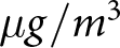 $\mu g/m^3$ and 35
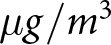 $\mu g/m^3$, relative to the air quality situation 24 hours before the warning. These findings are supported by our RD analysis, although with more optimistic reductions of particulate concentrations. Importantly, both methods reveal no statistically significant effects during air quality pre-emergencies.
When examining heterogeneous effects by time of day, the results indicate that these reductions are most pronounced at night, when temperatures are lower and wood-burning heaters are likely used more frequently. Moreover, improvements in air quality spill over into the following day due to the persistence of these pollutants in the atmosphere. We consider these findings as strong evidence of the effectiveness of the most severe air quality warning. However, while the program proves somewhat effective, it is important to note the persistently high average pollution levels in the city. It seems that prohibitions associated with the milder episodes are insufficient to produce a meaningful impact on pollution concentrations.
Our paper makes a significant contribution to the evaluation of environmental policy programs, particularly command-and-control strategies designed to reduce pollution in the Global South (Blackman et al., Reference Blackman, Li and Liu2018). While several studies have assessed the effectiveness of similar interventions to curb air pollution from stationary (e.g., Mullins and Bharadwaj, Reference Mullins and Bharadwaj2015) and mobile (e.g., Mullins and Bharadwaj, Reference Mullins and Bharadwaj2015; Rivera, Reference Rivera2021) sources, to the best of our knowledge, we are among the first to evaluate a policy aimed at restricting wood-burning practices. This provides valuable insights into the feasibility and potential impact of such interventions. Our study demonstrates the partial effectiveness of a policy mandate that limits the use of residential heating on days with critical air pollution levels, offering a potential solution to mitigate this form of pollution. However, our analysis also highlights the need for complementary approaches to reduce household pollution to health-safe levels, particularly in regions where wood heating and combustion are deeply rooted in local culture.
We also contribute to the growing body of literature evaluating environmental policies aimed at curbing air pollution in Chile (e.g., Troncoso et al., Reference Troncoso, de Grange and Cifuentes2012; Mullins and Bharadwaj, Reference Mullins and Bharadwaj2015; Rivera, Reference Rivera2021), with a particular focus on indoor air pollution (Schueftan and González, Reference Schueftan and González2015; Mardones and Cornejo, Reference Mardones and Cornejo2020b). Our study closely aligns with Mardones and Cornejo Reference Mardones and Cornejo(2020b), which assesses a similar policy in a southern Chilean city. However, a key distinction between our work and prior studies is our exclusive focus on causal identification, alongside an emphasis on the heterogeneity of impacts across different environmental episodes. This methodological approach enables a more nuanced understanding of the effectiveness and broader implications of environmental policy interventions.
The remainder of this document is organised as follows. In section 2, we describe the air quality situation of Los Angeles. We present the data in section 3 and the details of the empirical strategy in section 4. Results are presented in section 5, along with robustness analysis in sections 6 and 7. We offer a discussion of the main results in section 8, and conclude our analysis in section 9.
2. Background
Los Angeles is located approximately 514 km south of Santiago, the capital of Chile. The city’s primary source of air pollution is residential wood burning, which is mainly used for heating and cooking in households. It is estimated that more than 87 per cent of urban households in Los Angeles rely on wood as their main energy source for these activities, contributing to over 80 per cent of the PM pollution in the city.
In 2015, Los Angeles was recognised as one of the most polluted cities in Chile, with daily concentrations of PM2.5 and PM10 exceeding 150 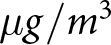 $\mu g/m^3$ and 50
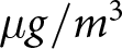 $\mu g/m^3$, respectively. In response, local authorities developed the Atmospheric Decontamination Plan, which aimed to improve environmental quality standards over the following decade Ministerio del Medio Ambiente 2019. The plan included a range of structural measures for pollution control across short-, medium- and long-term periods. Online appendix figure A1 shows the spatial area covered by these measures, along with the locations of the air quality stations used in our analysis.
This study focuses on a key short-term component of the Atmospheric Decontamination Plan, known as the Critical Episodes Management Program (PGEC). The PGEC involves the issuance of 24-hour environmental episodes, or air quality warnings, designed to reduce PM concentrations during periods of severe air pollution, particularly during the winter season (from April 1 to September 30). A comprehensive set of preventive and mitigation measures is triggered when pollution levels for either PM2.5 or PM10 (or both) exceed critical thresholds. In such cases, a three-tier system of environmental warnings is activated – alerts, pre-emergencies and emergencies – each of which prompts a series of restrictions on the use of wood-burning devices. Table 1 shows these thresholds, their corresponding pollution episode triggered in each case and whether these episodes imply wood-burning restrictions.Footnote 1
Environmental episodes and pollution levels

Table 1 Long description
The table has four columns: Air quality conditions, PM10, PM2.5 and Wood-burning restrictions. Row 1: Panel A: No episodes. Row 2: Good, 0–149, 0–50, No. Row 3: Decent, 150–194, 51–79, No. Row 4: Panel B: Episodes. Row 5: Alert, 195–239, 80–109, No. Row 6: Pre-emergency, 240–329, 110–169, Yes. Row 7: Emergency, greater than or equal to 330, greater than or equal to 170, Yes.
Notes: This table illustrates various air quality conditions, each triggering different air quality warnings (or episodes), along with the corresponding pollution concentrations for coarse particulate matter (PM10) and fine particulate matter (PM2.5). Pollution levels are measured in micrograms per cubic meter (µg/m3). The table also indicates whether a specific episode triggers or not wood-burning restrictions. Data sourced from the Ministry of the Environment.
During the mildest episode, alerts, authorities issue recommendations and advocate for responsible and efficient heating practices, yet no prohibitions are in place. When daily pollution concentrations exceed 110 µg/m 3 for PM2.5 or 240 µg/m 3 for PM10, a pre-emergency status is declared. This mandates the prohibition of wood-burning heaters, stoves and boilers emitting more than 30 µg/m3 of PM from 6 p.m. to midnight, along with traditional ovens throughout the entire day. In instances where daily concentrations surpass 170 µg/m 3 for PM2.5 or 330 µg/m 3 for PM10, an emergency is declared and the ban on wood-burning heaters, stoves and boilers is extended to 24 hours a day.
2.1. Enforcement and compliance with the policy
A comprehensive framework, overseen by the Ministry of Health and the Ministry of Environment, coordinates various actions to monitor air quality episodes. These oversight strategies include monitoring the use of open hearth fireplaces, regulating burning activities in wood-burning heaters and stoves, supervising the use of wood-burning heaters in commercial establishments and government buildings and controlling their usage in apartment buildings, among other measures. Since 2021, authorities have monitored approximately 24,956 homes, conducting detailed inspections in 402 of them and initiating investigations in 139 units. Non-compliant households face fines ranging from 63,000 Chilean pesos (approximately US$65D) to 1,200,000 Chilean pesos (approximately US$1,300).
Although we do not have data on the number of inspections since the creation of this program, figures for 2024 show that the regional Health Authority (SEREMI in Spanish) inspected 3,572 households out of a total of approximately 47,500 households in Los Angeles. Of these, only 229 (6.4 per cent) were inspected inside the residence, leading to 9 administrative proceedings. These numbers suggest that enforcement may be lacking in the city. This is likely the reason why concerns have been raised by the highest municipal authority regarding the effectiveness of the plan, highlighting the need for an empirical study on the causal impact of this command-and-control policy.
3. Data
We collect hourly pollution concentrations of PM10 and PM2.5, along with meteorological data (wind speed, temperature and humidity), from two air quality monitoring stations within the MACAM-2 network of the National Air Quality Information System (SINCA) for the period 2018–2022.Footnote 2 Additionally, data on days with wood-burning bans and forecasts for each environmental episode are obtained from the Regional Ministry of the Environment (SEREMI) of the Bío Bío Region. Appendix table A1 summarises the total number of episodes issued each year during the study period, highlighting that pre-emergencies are the most common type of air quality episode.
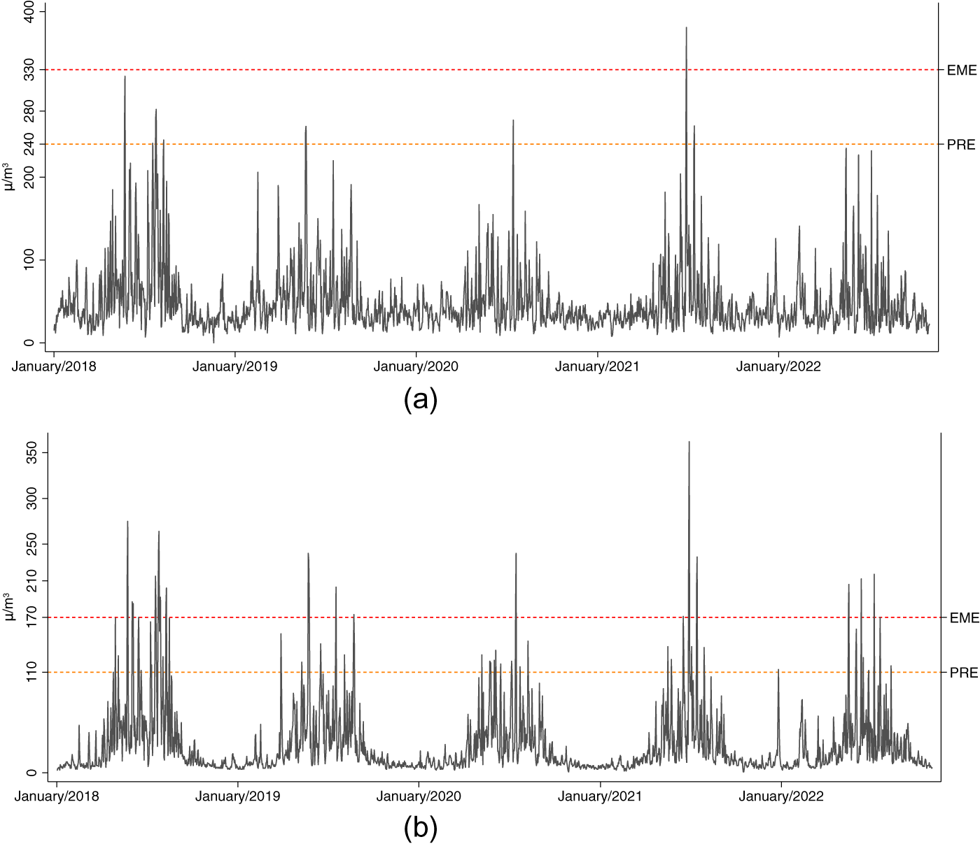
Figure 1 shows daily air pollution concentrations in Los Angeles from 2018 to 2022. Panel (a) displays average PM10 concentrations, while panel (b) exhibits average PM2.5 concentrations. Dashed lines indicate the thresholds for air quality episodes that trigger wood-burning prohibitions. The figure clearly illustrates a seasonal pattern, with higher pollution levels during the fall and winter months (from April to August). This seasonality can be attributed to two main factors. First, meteorological conditions, such as poor ventilation, low temperatures, thermal inversion and high pressure in the fall and winter, hinder the dispersion of pollutants, leading to higher atmospheric concentrations. Second, there is a notable increase in PM emissions in the city, primarily due to the use of wood for heating, which is more prevalent during these colder months.
PM10 and PM2.5 concentrations over time. (a) PM10. (b) PM2.5.

Figure 1 Long description
Panel (a) shows a line graph of PM10 concentrations in Los Angeles from January 2018 to January 2022. The x-axis represents time in years, labeled from January 2018 to January 2022. The y-axis represents PM10 concentration in microgram over meter superscript 3, ranging from 0 to 400. A solid line indicates PM10 data, with dashed lines marking thresholds labeled PRE at 240 and EME at 330. Peaks occur in fall and winter months, exceeding thresholds at times. Panel (b) displays PM2.5 concentrations over the same period. The x-axis is similarly labeled and the y-axis ranges from 0 to 350 microgram over meter superscript 3. A solid line shows PM2.5 data, with dashed lines marking thresholds labeled PRE at 110 and EME at 170. Seasonal peaks are evident, with exceedances during colder months. Both panels illustrate higher pollution levels in fall and winter, highlighting seasonal variations and air quality concerns.
Additionally, figure 1 highlights that, during certain periods, daily PM10 concentrations (panel (a)) not only exceed the World Health Organization recommended limit of 50 µg/m3 for a 24-hour average but also surpass the local standard in Chile of 150 µg/m3 for a 24-hour average. This issue is even more pronounced for PM2.5 concentrations (panel (b)), further emphasising the significant health risks posed by air pollution in this city.
To better understand patterns in air pollution concentrations, appendix figures A2 and A3 show the hourly profiles of both PM10 and PM2.5 concentrations on days with pre-emergencies and emergencies, respectively. In addition to plotting pollution concentrations during the day with declared episodes, that is, when wood-burning restrictions are imposed, we also include the average concentrations from the day before the episode, which corresponds to the day when the announcement is made.
When comparing appendix figures A2 and A3, a few key patterns emerge. First, pollution concentrations are noticeably higher 24 hours before an emergency (figure A3) compared to those before a pre-emergency (figure A2). Second, both figures show a clear hourly cycle, with pollution levels rising during the evening hours, particularly after 6 p.m. and peaking between 8 p.m. and midnight. This pattern coincides with the time when most people are indoors, likely using their heaters. Third, in the case of pre-emergencies (figure A2), pollution concentrations are typically lower on the day preceding the episode than on the episode day itself. In contrast, during emergencies, concentrations tend to be higher on the day before the episode than during it (figure A3), suggesting that air pollution may be more effectively reduced during more severe events.
The descriptive statistics on hourly pollution concentrations, presented in appendix table A2, support this conclusion. Panel A shows the hourly average concentrations for the entire sample period, while panels B through E display 24-hour average concentrations for the days before and during an episode. For example, panels D and E show that pollution levels decrease significantly, from 111 µg/m3 to 72 µg/m3 for PM10 and from 121 µg/m3 to 84 µg/m3 for PM2.5, during the emergency period. These observations suggest that the policy under evaluation may have a more pronounced impact under the strictest wood-burning restrictions, namely during emergencies. Appendix table A3 presents similar descriptive statistics for weather variables, which are also considered in the empirical analysis.
4. Methods
In this work, we evaluate the causal impact of wood-burning restrictions, triggered by air quality warnings (i.e., pre-emergency and emergency episodes), on hourly concentrations of PM in the city of Los Angeles, Chile. To this, we draw insights from two distinct econometric approaches. First, we exploit the pre-policy period (i.e., pre-2018) to define an estimation approach in double differences (DID) that uses days before the policy as the control group. We complement this approach with an RD specification that uses time as the running variable and environmental episodes as thresholds. Further details on these methodologies are provided below.
4.1. Pre-policy period and estimation in double differences
Our first approach builds on the policy’s design and the data availability during a pre-policy period in Los Angeles, which enables us to construct a valid counterfactual for episode days during the policy period. Specifically, we use publicly available hourly pollution data from a single station covering the years 2013 to 2017. Leveraging the policy design, we identify pre-policy days that, due to their high PM concentrations, would have triggered an episode had the policy under analysis been in place. We compare the hourly pollution concentrations between days with episodes and days before an episode (i.e., 1 or 2 days before) before and after the policy implementation.Footnote 3
Let Pit represent average pollution concentrations (logged) in station i during hour t. We specifically estimate variations of the following equation:
 \begin{equation}
P_{it}=\gamma_{0} + \gamma_1 1[Episode]_t + \gamma_{2}1[Post-2018]_i\times 1[Episode]_t + {\bf{X_{it}}} \lambda + \delta_i + \mu_{t} + \eta_{it},
\end{equation}
where  $1[Post-2018]$ is an indicator that takes 1 if pollution record at station i during hour t belongs to the treated (post-2018) period and 0 if belongs to the control (pre-2018) period, and the indicator
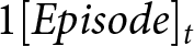 $1[Episode]_t$ indicates whether an episode (i.e., pre-emergency or emergency) was issued (or should have been issued) at hour t (and 0 for days before an episode). Equation (1) also includes the vector
 ${\bf{X_{it}}}$, a set of control variables known to affect air pollution concentrations such as meteorological variables (temperature, wind speed and relative humidity), δi that represents station-fixed effects, µt that represents several time fixed effects (year, month, day of the week and hour of the day – all included simultaneously) and ηit that represents the idiosyncratic error term. We estimate equation (1) using ordinary least squares (OLS), clustering standard errors at the station level.
Our parameter of interest, γ 2, captures the difference in pollution levels between hours of days with episodes and hours of days preceding an episode, before and after the policy implementation. In the absence of the policy intervention, and conditional on our observable controls, we would not expect significant differences in pollution levels across these groups of days before and after the policy implementation. Therefore, any such difference can be attributed to the policy itself. Thus, the parameter γ 2 provides a reasonable approximation of the causal effect of the policy intervention.
The previous argument, however, relies on the common trends assumption for air pollution concentrations in both the treatment and control groups. Appendix figures A4 and A5 assess this assumption for air quality during pre-emergencies and emergencies, respectively, by showing the hourly average PM concentrations in Los Angeles during the pre- and post-policy periods, 48 hours before and after each of these episodes. As shown, the two trends closely follow a similar pattern before pollution levels reach the thresholds that, under the policy design, would trigger an environmental episode.
4.2. Regression discontinuity
We complement the previous specification with a sharp RD design that uses time as the running variable and the issuance of an environmental episode as the thresholds. This treatment takes the value one if an episode was issued on a specific day, and zero otherwise. Our key identifying assumption here is that, in the absence of the treatment (i.e., an environmental episode), pollution concentrations should change smoothly around the threshold (i.e., the issuance date). We estimate variations of the following equation:
 \begin{equation}
P_{it}= \beta_{0}+\beta_{1}1[Episode]_{t}+\beta_{2}f(x)+\beta_{3}1[Episode]_{t}f(x)+ {\bf{X_{it}}}\lambda +\delta_{i}+\mu _{t}+\varepsilon_{it},
\end{equation}
where 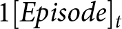 $1[Episode]_t$ is a binary variable that takes the value of 1 if hour t belongs to a day with an episode (i.e., pre-emergencies or emergencies) and 0 otherwise, f(x) a first-order polynomial function and
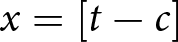 $x = [t-c]$ is the assignment indicating the number of hours before and after an episode, and c represents the cut-off, that is, the first hour of the day with an episode. We normalise the cut-off to 0, so negative and positive values for x represent hours before and after an event. Similar to equation (1), equation (2) also includes a vector of controls
 ${\bf{X_{it}}}$, station-fixed effects (δi), time-fixed effects (µt) and an idiosyncratic error term defined as ɛit.
Our parameter of interest in equation (2) is β 1, which captures the difference in hourly pollution concentrations before and after the issuance of an episode. A negative and statistically significant β 1 would provide evidence of the effectiveness of wood-burning restrictions, triggered by environmental episodes, in reducing hourly pollution concentrations. We estimate equation (2) using OLS, clustering standard errors at the station level. In our robustness analysis, we employ Newey-West standard errors to account for any potential serial correlation in the pollution data.Footnote 4
It is important to note that the choice of the functional form for the adjustment polynomial in the RD specifications is critical. By using an adjustment polynomial, we impose a particular structure on the relationship between the running variable x and the outcome variable Pit. If the true relationship between these variables does not align well with the chosen polynomial’s functional form, the model may fail to accurately capture the underlying dynamics, potentially leading to biased estimates. With this in mind, we explore both a first-order and a quadratic functional form to model f(x), although our preferred specification remains the more conservative linear form.
5. The effectiveness of wood-burning bans
5.1. Pre-policy period and difference-in-difference estimation
Our first approach estimates a DID specification to capture the causal effect of wood-burning bans, which are triggered by environmental episodes, aimed at reducing air pollution on days with critical air quality levels. We conduct this DID analysis using pre-policy (pre-2018) hourly pollution data for Los Angeles. Leveraging the policy design, we identify pre-policy days that, due to elevated PM concentrations, would have triggered an air quality episode had the policy been in effect. As previously defined by equation (1), we use these pre-policy days to later compare air pollution records between days with an episode (or that should have had one) and days preceding an episode, before and after the policy implementation. The results of estimating this equation are presented in table 2 using 24 hours and 48 hours before an episode as two different specifications for the control group.
The impact of pre-emergency and emergency episodes on pollution concentrations: a DID approach

Table 2 Long description
The table has six columns: Using 24 hrs before as controls PM10, Using 24 hrs before as controls PM2.5, Using 48 hrs before as controls PM10, Using 48 hrs before as controls PM2.5, Controls, Time fixed-effects. Row 1: 1[Post-2018] times 1[Pre-emergencies] 0.0133 (0.0406); -0.0357 (0.0434); 0.0350 (0.0292); -0.0133 (0.0310). Row 2: N 3,935; 3,935; 6,972; 6,970. Row 3: 1[Post-2018] times 1[Emergencies] -0.229 (0.0760); -0.180 (0.0787); -0.286 (0.0616); -0.123 (0.0592). Row 4: N 1,128; 1,185; 2,057; 2,046. Row 5: Controls check mark; check mark; check mark; check mark. Row 6: Time fixed-effects check mark; check mark; check mark; check mark. Row 7: Sample Mean Pre-emergencies 195.7; 79.36; 192.8; 68.6. Row 8: Sample Mean Emergencies 226.7; 196.4; 171.2; 147.7.
Notes: This table shows the impact of air quality warnings on (logged) hourly concentrations of PM10 and PM2.5 in Los Angeles using a DID estimator. All regressions include weather controls (temperature, wind speed, humidity), and station and time fixed (year, month, day of the week and hour of the day). Sample means are 24-hour or 48-hour averages before the corresponding episode. Clustered standard errors by station in parentheses.
The results in table 2 indicate that wood-burning restrictions triggered by air quality pre-emergencies appear insufficient to reduce pollution levels on these high-risk days. When using the 24 hours prior to an episode (or pseudo-episode) as the control period, we find that pre-emergencies are associated with a slight increase in PM10 and a decrease in PM2.5 concentrations; however, neither estimate is statistically significant. Similar patterns emerge when the control period is extended to 48 hours before an episode.
In contrast, the findings for air quality emergencies tell a different story. Only this most severe warning appears effective in reducing PM concentrations. Using the day immediately preceding an episode as a control, our results show that wood-burning restrictions triggered by air quality emergencies reduce PM10 and PM2.5 concentrations by 23 and 18 per cent, respectively. These effects translate to reductions of 52 and 35 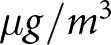 $\mu g/m^3$ relative to average pollution levels observed the day before these episodes. Expanding the control window to two days yields similar results, although the estimated effects are slightly smaller in magnitude in the case of PM2.5.
Thus far, the results presented in table 2 strongly suggest that wood-burning restrictions are effective in reducing both fine and coarse PM concentrations, but only when triggered by air quality emergencies. In contrast, when these restrictions are implemented during milder episodes, such as pre-emergencies, they are insufficient to lower pollution levels in the city. It is important to note that while pre-emergencies trigger biomass burning restrictions only from 6 p.m. to midnight, environmental emergencies, when triggered, impose these prohibitions throughout the entire day, which naturally results in more substantial effects.
Nonetheless, the specific hours of restriction matter. In fact, as shown in appendix figure A3, relative to the day before emergencies, pollution concentrations appear visually lower not only before 5 p.m. but also early in the morning, between 6 and 7 a.m. This pattern suggests that the impact of wood-burning restrictions may extend beyond the designated evening hours, potentially improving air quality throughout the day, including late at night. Moreover, if households primarily burn wood during specific times – such as in the evening for heating or cooking – we would expect the most pronounced effects to occur during those periods. We examine these temporal dynamics in greater detail below, identifying the hours during which pollution reductions are most significant and assessing whether these improvements persist into subsequent days.
5.1.1. Heterogeneous effects by hours of the day
In this section, we investigate whether the results presented in table 2 mask heterogeneous effects across different times of the day. To do so, we re-estimate equation (1), allowing the treatment effects to vary by time blocks. Specifically, we examine pollution reductions in 3-hour intervals, using the 3–6 p.m. window, the period immediately preceding the onset of restrictions during pre-emergencies, as the reference category.
Our findings in table 3 indicate that wood-burning prohibitions are most effective during the evening and late-night hours. In the case of pre-emergencies, air quality appears to improve primarily between 6 p.m. and midnight, the period during which these restrictions are active, although some of these effects are only weakly significant when using a 24-hour comparison window. After midnight, however, air quality seems to deteriorate, and this pattern may persist until around noon the following day. One possible explanation is the persistence of PM in the atmosphere, which may take longer to disperse despite the restrictions in place.
The impact of air quality episodes on hourly pollution concentrations: heterogeneous effects by hour of the day using a DID approach

Table 3 Long description
The table has columns: Hours, Pre-emergency 24 Hours PM10, Pre-emergency 24 Hours PM2.5, Pre-emergency 48 Hours PM10, Pre-emergency 48 Hours PM2.5, Emergency 24 Hours PM10, Emergency 24 Hours PM2.5, Emergency 48 Hours PM10, Emergency 48 Hours PM2.5. There are 7 hour-interval rows plus 4 additional rows for N, Controls, Station fixed-effects and Time fixed-effects. The hour intervals listed are 0:00 4 h < 3:00; 3:00 4 h < 6:00; 6:00 4 h < 9:00; 9:00 4 h < 12:00; 12:00 4 h < 15:00; 18:00 4 h < 21:00; 21:00 4 h 4 23:00. No row is shown for 15:00 4 h < 18:00. Row 1: 0:00 4 h < 3:00. Pre-emergency 24 Hours PM10 0.169 left parenthesis 0.103 right parenthesis; Pre-emergency 24 Hours PM2.5 0.140 left parenthesis 0.110 right parenthesis; Pre-emergency 48 Hours PM10 0.140 left parenthesis 0.0569 right parenthesis; Pre-emergency 48 Hours PM2.5 0.0892 left parenthesis 0.0604 right parenthesis; Emergency 24 Hours PM10 -0.224 left parenthesis 0.168 right parenthesis; Emergency 24 Hours PM2.5 -0.377 left parenthesis 0.148 right parenthesis; Emergency 48 Hours PM10 0.111 left parenthesis 0.135 right parenthesis; Emergency 48 Hours PM2.5 -0.205 left parenthesis 0.110 right parenthesis. Row 2: 3:00 4 h < 6:00. Pre-emergency 24 Hours PM10 0.213 left parenthesis 0.106 right parenthesis; Pre-emergency 24 Hours PM2.5 0.218 left parenthesis 0.114 right parenthesis; Pre-emergency 48 Hours PM10 0.193 left parenthesis 0.0584 right parenthesis; Pre-emergency 48 Hours PM2.5 0.186 left parenthesis 0.0618 right parenthesis; Emergency 24 Hours PM10 -0.143 left parenthesis 0.174 right parenthesis; Emergency 24 Hours PM2.5 -0.262 left parenthesis 0.152 right parenthesis; Emergency 48 Hours PM10 0.193 left parenthesis 0.140 right parenthesis; Emergency 48 Hours PM2.5 -0.126 left parenthesis 0.112 right parenthesis. Row 3: 6:00 4 h < 9:00. Pre-emergency 24 Hours PM10 -0.106 left parenthesis 0.106 right parenthesis; Pre-emergency 24 Hours PM2.5 -0.0822 left parenthesis 0.114 right parenthesis; Pre-emergency 48 Hours PM10 0.112 left parenthesis 0.0587 right parenthesis; Pre-emergency 48 Hours PM2.5 0.0849 left parenthesis 0.0622 right parenthesis; Emergency 24 Hours PM10 -0.315 left parenthesis 0.174 right parenthesis; Emergency 24 Hours PM2.5 -0.147 left parenthesis 0.152 right parenthesis; Emergency 48 Hours PM10 -0.00628 left parenthesis 0.142 right parenthesis; Emergency 48 Hours PM2.5 -0.125 left parenthesis 0.112 right parenthesis. Row 4: 9:00 4 h < 12:00. Pre-emergency 24 Hours PM10 0.0687 left parenthesis 0.106 right parenthesis; Pre-emergency 24 Hours PM2.5 0.0862 left parenthesis 0.114 right parenthesis; Pre-emergency 48 Hours PM10 0.132 left parenthesis 0.0579 right parenthesis; Pre-emergency 48 Hours PM2.5 0.117 left parenthesis 0.0613 right parenthesis; Emergency 24 Hours PM10 -0.0499 left parenthesis 0.174 right parenthesis; Emergency 24 Hours PM2.5 -0.149 left parenthesis 0.153 right parenthesis; Emergency 48 Hours PM10 0.00426 left parenthesis 0.137 right parenthesis; Emergency 48 Hours PM2.5 -0.125 left parenthesis 0.113 right parenthesis. Row 5: 12:00 4 h < 15:00. Pre-emergency 24 Hours PM10 -0.0484 left parenthesis 0.111 right parenthesis; Pre-emergency 24 Hours PM2.5 -0.0147 left parenthesis 0.119 right parenthesis; Pre-emergency 48 Hours PM10 0.0283 left parenthesis 0.0590 right parenthesis; Pre-emergency 48 Hours PM2.5 0.0692 left parenthesis 0.0625 right parenthesis; Emergency 24 Hours PM10 0.0611 left parenthesis 0.183 right parenthesis; Emergency 24 Hours PM2.5 -0.0760 left parenthesis 0.158 right parenthesis; Emergency 48 Hours PM10 0.197 left parenthesis 0.140 right parenthesis; Emergency 48 Hours PM2.5 0.0838 left parenthesis 0.114 right parenthesis. Row 6: 18:00 4 h < 21:00. Pre-emergency 24 Hours PM10 -0.167 left parenthesis 0.111 right parenthesis; Pre-emergency 24 Hours PM2.5 -0.218 left parenthesis 0.119 right parenthesis; Pre-emergency 48 Hours PM10 -0.133 left parenthesis 0.0589 right parenthesis; Pre-emergency 48 Hours PM2.5 -0.175 left parenthesis 0.0624 right parenthesis; Emergency 24 Hours PM10 -0.525 left parenthesis 0.183 right parenthesis; Emergency 24 Hours PM2.5 -0.396 left parenthesis 0.158 right parenthesis; Emergency 48 Hours PM10 -0.512 left parenthesis 0.140 right parenthesis; Emergency 48 Hours PM2.5 -0.402 left parenthesis 0.114 right parenthesis. Row 7: 21:00 4 h 4 23:00. Pre-emergency 24 Hours PM10 -0.326 left parenthesis 0.110 right parenthesis; Pre-emergency 24 Hours PM2.5 -0.388 left parenthesis 0.118 right parenthesis; Pre-emergency 48 Hours PM10 -0.144 left parenthesis 0.0589 right parenthesis; Pre-emergency 48 Hours PM2.5 -0.183 left parenthesis 0.0624 right parenthesis; Emergency 24 Hours PM10 -0.478 left parenthesis 0.183 right parenthesis; Emergency 24 Hours PM2.5 -0.298 left parenthesis 0.157 right parenthesis; Emergency 48 Hours PM10 -0.488 left parenthesis 0.141 right parenthesis; Emergency 48 Hours PM2.5 -0.375 left parenthesis 0.114 right parenthesis. Row 8: N. Pre-emergency 24 Hours PM10 3935; Pre-emergency 24 Hours PM2.5 3935; Pre-emergency 48 Hours PM10 6972; Pre-emergency 48 Hours PM2.5 6970; Emergency 24 Hours PM10 1,128; Emergency 24 Hours PM2.5 1,185; Emergency 48 Hours PM10 2,057; Emergency 48 Hours PM2.5 2,046. Row 9: Controls. Pre-emergency 24 Hours PM10 check mark; Pre-emergency 24 Hours PM2.5 check mark; Pre-emergency 48 Hours PM10 check mark; Pre-emergency 48 Hours PM2.5 check mark; Emergency 24 Hours PM10 check mark; Emergency 24 Hours PM2.5 check mark; Emergency 48 Hours PM10 check mark; Emergency 48 Hours PM2.5 check mark. Row 10: Station fixed-effects. Pre-emergency 24 Hours PM10 check mark; Pre-emergency 24 Hours PM2.5 check mark; Pre-emergency 48 Hours PM10 check mark; Pre-emergency 48 Hours PM2.5 check mark; Emergency 24 Hours PM10 check mark; Emergency 24 Hours PM2.5 check mark; Emergency 48 Hours PM10 check mark; Emergency 48 Hours PM2.5 check mark. Row 11: Time fixed-effects. Pre-emergency 24 Hours PM10 check mark; Pre-emergency 24 Hours PM2.5 check mark; Pre-emergency 48 Hours PM10 check mark; Pre-emergency 48 Hours PM2.5 check mark; Emergency 24 Hours PM10 check mark; Emergency 24 Hours PM2.5 check mark; Emergency 48 Hours PM10 check mark; Emergency 48 Hours PM2.5 check mark. Across the listed hour blocks, the largest positive coefficients shown are 0.218 for Pre-emergency 24 Hours PM2.5 at 3:00 4 h < 6:00 and 0.213 for Pre-emergency 24 Hours PM10 at 3:00 4 h < 6:00 and 0.197 for Emergency 48 Hours PM10 at 12:00 4 h < 15:00. The most negative coefficients shown are -0.525 for Emergency 24 Hours PM10 at 18:00 4 h < 21:00, -0.512 for Emergency 48 Hours PM10 at 18:00 4 h < 21:00 and -0.402 for Emergency 48 Hours PM2.5 at 18:00 4 h < 21:00.
Notes: This table presents heterogeneous hourly effects of the impact of air quality pre-emergencies and emergencies on hourly PM concentrations using a DID estimator. All regressions include weather controls (temperature, wind speed, humidity), and station and time fixed (year, month, day of the week and hour of the day). Clustered standard errors by station in parentheses.
In contrast, emergencies exhibit a clearer pattern of air quality improvement starting at 6 p.m. Across the two pollutants, these more severe episodes are associated with substantial reductions in pollution levels during the evening and late-night hours. Although emergency episodes are officially in effect for 24 hours, the most pronounced and statistically significant declines occur during the times of day when polluting activities are likely to be most intense, particularly in the late evening. Notably, these improvements persist into the early hours of the following day (midnight to 3 a.m.), although reductions observed during this period are modest, and some of them are not statistically significant.
5.1.2. Long-lasting effects
Although modest, the air quality improvements observed during hours with minimal expected biomass burning activity (e.g., midnight to 3 a.m.) suggest some persistence in pollution reduction. This raises the question of whether the policy’s effects extend beyond the immediate hours following an episode. A key characteristic of PM is its ability to remain suspended in the air for extended periods, potentially influencing air quality beyond the initial 24-hour window. This makes it plausible that certain air quality warnings could have long-lasting effects.
With this in mind, appendix table A5 presents the results of our DID baseline equation but using now 24-hour lead pollution concentrations (i.e.,  $P_{it+24}$, pollution levels measured one day after the episode). Once again, we find that only air quality emergencies lead to reductions in pollution concentrations the day after an episode. However, these reductions are somewhat more optimistic, ranging from 21 to 23 per cent. Interestingly, with this approach, we also observe a reduction in pollution concentrations that extends beyond the next day, with effects spilling over into two days (48 hours) after the episode, particularly for PM10. This extended impact suggests a longer-term health benefit for the population, highlighting a substantial decrease in both pollutants over an extended period.
5.2. Regression discontinuity
To corroborate our previous estimates, we adopt an alternative empirical strategy that leverages the structure of the policy and the timing of episode issuance. Specifically, we implement an RD design to capture the local average treatment effects of wood-burning bans, which are triggered by environmental episodes aimed at reducing air pollution on days with critical air quality levels.
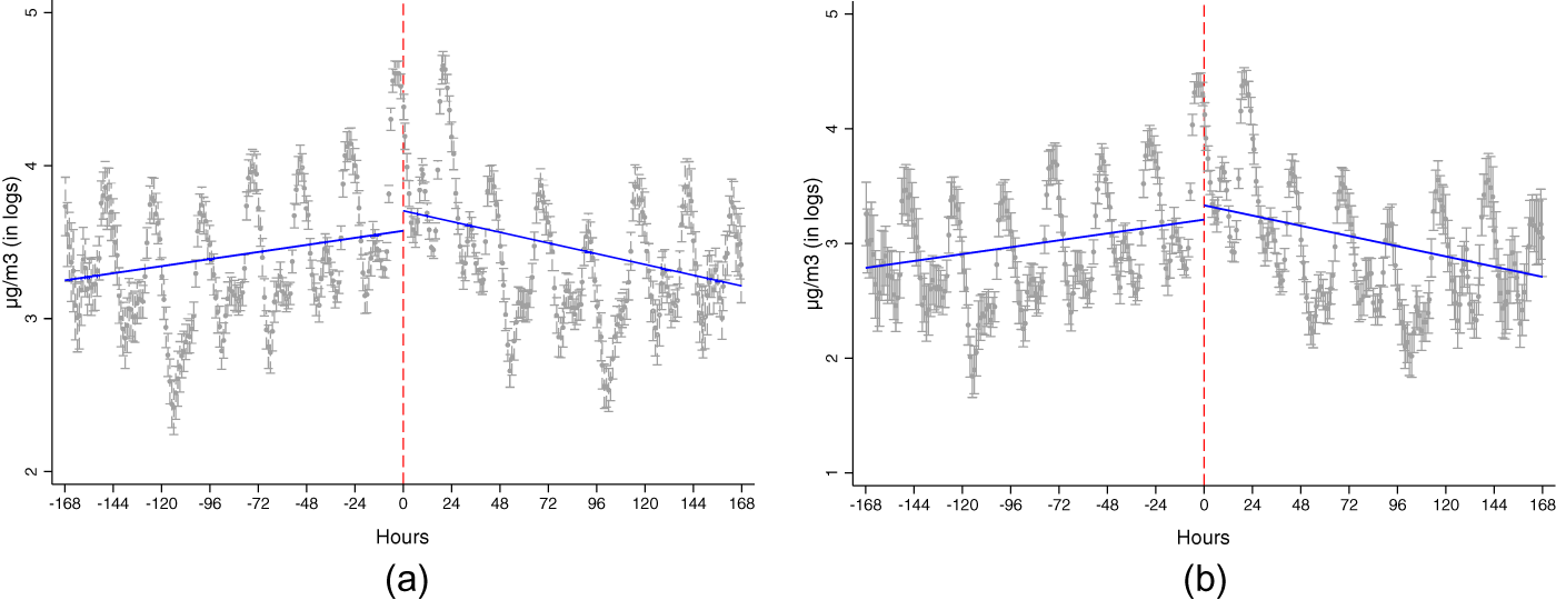
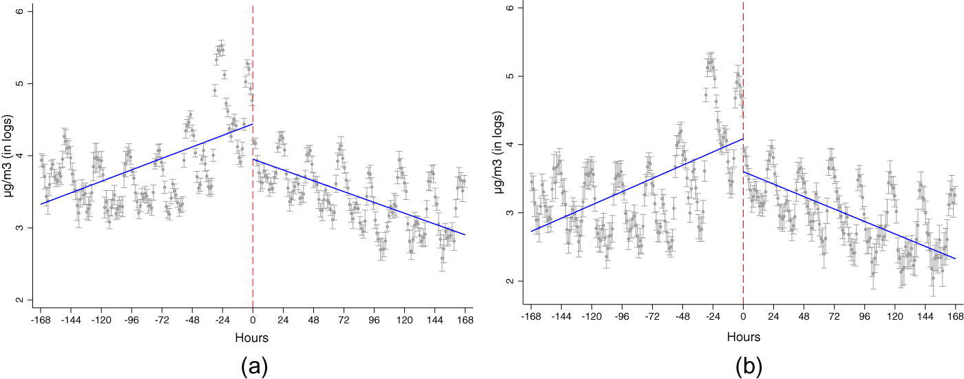
We begin by examining data-driven plots in figures 2 and 3, which display hourly concentrations of PM10 and PM2.5 (in logs) for the seven days before and after air quality pre-emergencies and emergencies, respectively. Both figures include a linear fit on either side of the corresponding threshold. As expected, air pollution concentrations consistently increase just before the issuance of an episode, particularly before an emergency (see figure 3). However, in the case of pre-emergencies, the issuance of the episode does not appear to significantly reduce pollution concentrations. Based on the linear fit, we observe a slight increase in average concentrations after the episode, but this difference is not statistically significant.
The impact of pre-emergency episodes on hourly pollution concentrations: a regression discontinuity approach. (a) PM10. (b) PM2.5.

Figure 2 Long description
The image contains two scatter plots labeled (a) and (b), comparing hourly pollution concentrations before and after episodes. The horizontal axis is labeled Hours, ranging from negative 168 to 168. The vertical axis is labeled microgram per meter superscript 3 in logs, ranging from 2 to 5 in plot (a) and 1 to 5 in plot (b). Both plots feature a segmented fitted line intersecting at Hour 0, with the line rising before Hour 0 and falling after. Error bars indicate variability in the data points. Plot (a) represents PM concentrations, while plot (b) represents PM.pre-emergency concentrations. The fitted line in both plots is blue and the vertical dashed line at Hour 0 marks the episode threshold. Notable peaks occur near Hour 0, with higher concentrations observed between Hour negative 24 and Hour 24. The purpose is to illustrate changes in pollution levels before and after episodes, highlighting the impact of emergencies on air quality.
The impact of emergency episodes on hourly pollution concentrations: a regression discontinuity approach. (a) PM10. (b) PM2.5.

Figure 3 Long description
The image A showing a scatter plot labeled (a). The x-axis is labeled Hours, with tick labels at minus 168, minus 144, minus 120, minus 96, minus 72, minus 48, minus 24, 0, 24, 48, 72, 96, 120, 144, 168. The y-axis is labeled microgram per meter cubed (in logs), with tick labels 2, 3, 4, 5, 6. A vertical dashed line is drawn at 0 hours. Many gray points with vertical error bars are plotted across the full x-axis range. A blue fitted line segment increases from about 3.3 at minus 168 hours to about 4.4 at 0 hours. A second blue fitted line segment decreases from about 4.0 at 0 hours to about 2.9 at 168 hours. The image B showing a scatter plot labeled (b). The x-axis is labeled Hours, with tick labels at minus 168, minus 144, minus 120, minus 96, minus 72, minus 48, minus 24, 0, 24, 48, 72, 96, 120, 144, 168. The y-axis is labeled microgram per meter cubed (in logs), with tick labels 2, 3, 4, 5, 6. A vertical dashed line is drawn at 0 hours. Many gray points with vertical error bars are plotted across the full x-axis range. A blue fitted line segment increases from about 2.8 at minus 168 hours to about 4.0 at 0 hours. A second blue fitted line segment decreases from about 3.6 at 0 hours to about 2.4 at 168 hours.
In contrast, for emergencies, a different pattern emerges. The results in figure 3 suggest that environmental emergencies effectively reduce hourly concentrations of both PM10 and PM2.5 at the threshold. The corresponding formal test for this visual observation is presented in appendix table A6 for the case of pre-emergencies and in table 4 for the case of emergencies. Columns (1) to (3) represent different specifications of the original equation, with both linear and quadratic polynomial fits on either side of the threshold. The results in column (3), using a linear fit, represent our preferred specification throughout the remaining RD analysis.
The impact of emergency episodes on hourly pollution concentrations: a regression discontinuity approach

Table 4 Long description
The table has six columns labeled (1) to (6) under Linear fit and Quadratic fit. Panel A: PM10. Row 1: 1[Emergency] values are -0.577 (0.232), -0.802 (0.310), -0.403 (0.146), -0.563 (0.241), -0.545 (0.209), -0.400 (0.203). Row 2: N is 6,333 for all columns. Panel B: PM2.5. Row 1: 1[Emergency] values are -0.979 (0.550), -0.788 (0.472), -0.265 (0.0761), -0.730 (0.436), -0.507 (0.431), -0.123 (0.117). Row 2: N is 6,333 for all columns. Controls are present in columns (2) to (6). Station fixed-effects are present in columns (3) to (6). Time fixed-effects are present in columns (4) to (6). Statistics Panel A: Mean left (micrograms per cubic meter) is 71.39 for all columns. Mean right (micrograms per cubic meter) is 38.18 for all columns. Bandwidth (hours) values are 24.93, 15.69, 9.025, 50.91, 69.05, 23.82. Statistics Panel B: Mean left (micrograms per cubic meter) is 56.70 for all columns. Mean right (micrograms per cubic meter) is 19.88 for all columns. Bandwidth (hours) values are 16.98, 21.27, 15.28, 57.92, 51.73, 31.00.
Notes: This table presents the impact of air quality emergencies on the (logged) hourly average concentrations of PM. Panel A shows the results for PM10. Panel B shows the results for PM2.5. All regressions include weather controls (temperature, wind speed, humidity), and station and time fixed (year, month, day of the week and hour of the day). Optimal bandwidth using MSE minimisation (Calonico et al., Reference Calonico, Cattaneo and Titiunik2014). Clustered standard errors by station in parentheses.
The results in appendix table A6 align with those shown in figure 2 for air quality pre-emergencies. Wood-burning restrictions triggered by these warnings seem insufficient to reduce pollution levels during these critical days, regardless of the polynomial fit applied. In contrast, the findings in table 4 for emergencies suggest different insights. As shown in figure 3, air quality emergencies are effective in reducing pollution concentrations. In column (1) of panel A, using a linear fit, we observe that triggering an emergency leads to a reduction of PM10 concentrations by more than 50 per cent. After including controls, this effect decreases to 40 per cent in our preferred specification in column (3). Relative to the sample mean, this reduction is approximately 29 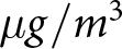 $\mu g/m^3$ of PM10 per hour, based on the pre-episode values. This result holds consistently whether a linear or quadratic polynomial fit is applied on either side of the threshold.
Similar patterns are observed for PM2.5 in panel B. The results in column (3) indicate that air quality emergencies reduce hourly PM2.5 concentrations by 26.5 per cent on days with episodes, which corresponds to a decrease of 15 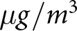 $\mu g/m^3$ per hour. A quadratic fit supports this reduction, though statistical significance is lost in some specifications. In conclusion, the results in tables A6 and 4 align with our previous DID results and suggest that only air quality emergencies have been effective in reducing air pollution concentrations.
As with the DID specification, we also examine heterogeneous effects by hour of the day. Appendix table A7 presents the results of this analysis, where we assess pollution reductions in 3-hour intervals using the 3–6 p.m. block as the reference category. Our findings indicate that wood-burning prohibitions are most effective during the evening and late-night hours. For emergencies, statistically significant reductions in air pollution are observed primarily in the early morning hours (between 3 a.m. and 6 a.m.) and continue through the morning (from 9 a.m. to noon). Although modest reductions are also detected during the evening, these effects tend to dissipate after 9 p.m.
One possible explanation for this pattern is the persistence of PM in the atmosphere, as previously discussed. This persistence may account for the notable reduction in PM10 concentrations observed between midnight and 3 a.m. during emergencies. While most wood-burning activity likely occurs before midnight, the delayed dispersion of pollutants may result in a lagged effect, with measurable improvements in air quality emerging several hours later.
Regarding long-lasting effects, appendix table A8 shows the results for our baseline RD equation using 24-hour lead pollution concentrations (i.e., pollution levels measured one day after the episode). Consistent with the main results, the findings in table A8 show that the effects of air quality emergencies extend slightly beyond 24 hours. Specifically, we observe a reduction of 31–32 per cent in both coarse and fine PM concentrations when using a linear polynomial fit. Table A8 also shows that no lead effects are observed for pre-emergencies, reinforcing the idea that the shorter 6-hour window of biomass burning prohibitions may not be sufficient to produce substantial improvements in air quality.
6. Additional estimations
In this section, we conduct a series of additional estimations to further examine whether the previous findings accurately capture the effectiveness of the policy. First, we investigate whether the observed effects are driven by the sequential issuance of multiple episodes or if they can be attributed to a single one. Second, we analyse the impact of air quality alerts. As noted earlier, these episodes are intended solely to inform the public about air quality conditions but do not trigger any behavioural restrictions. Exploring the potential effects of these alerts serves as a placebo test, helping to validate the robustness of the previous estimates. Next, we test for potential mean reversion in the outcome variable, given the time series nature of the data, to assess whether this might be influencing our RD estimation. Finally, we incorporate the time series characteristic of our main variable, air pollution, into our estimation and, for better inference, we repeat the previous estimations using Newey-Standard errors.
6.1. Isolated episodes
During the study period, certain air quality episodes may occur consecutively, meaning that either pre-emergencies or emergencies can happen on two consecutive days. In such cases, the results from previous analyses might not solely reflect the impact of a single episode but rather an accumulative effect, especially when lead impacts are present, as previously demonstrated. To test this possibility, we repeat our main empirical analysis but focus only on isolated episodes, excluding consecutive ones.
Appendix tables A9 and A10 present the results of this analysis using both the DID and RD approaches, respectively. Both methods reinforce the earlier findings regarding the effectiveness of emergencies in improving air quality. Specifically, table A9 shows that these severe episodes reduce PM10 and PM2.5 concentrations by 26 and 19 per cent, respectively, when using the 24 hours prior to an episode as the control period. Similar reductions are observed when using a 48-hour control window. In contrast, pre-emergencies do not show statistically significant reductions in either PM10 or PM2.5 levels. Overall, the results in table A9 suggest that air quality emergencies are an effective tool for reducing pollution and that the previous results do not obey an accumulation of bans over time. The RD estimates in table A10 yield comparable results, particularly for PM10.
6.2. Air quality alerts
As previously discussed, air quality alerts are the mildest type of environmental episode and, unlike pre-emergencies and emergencies, they do not impose wood-burning bans. Instead, they provide health recommendations and encourage responsible use of household heaters. Given the nature of these alerts, we would not expect them to have a significant impact on air pollution concentrations.Footnote 5
To test this, we estimate equation (2) for the case of hours of days with environmental alerts. The results, presented in appendix table A11, show almost no effect on PM concentrations in the city. Using our preferred estimation in column (3) along with a linear fit, we find that air quality alerts lead to no significant change in pollution levels. These results further validate our previous findings.
6.3. Mean reversion
To ensure that the counterfactual outcomes evolve smoothly over time, we analyse the neighbouring city of Nacimiento, which did not receive the treatment. As shown in figure A1, Los Angeles is located just 30 km northeast of Nacimiento. Despite their proximity, Nacimiento does not implement wood-burning restrictions during periods of critical air pollution, although it likely experiences similar weather conditions and cultural characteristics. This makes it an ideal candidate for testing whether our previous findings are merely a product of data characteristics, such as reversion to the mean.
We leverage the policy design by identifying days in Nacimiento that would have been classified as pre-emergencies or emergencies had the city been subject to the same restrictions as Los Angeles. Once these days are identified, we estimate equation (2) using Nacimiento’s pollution data to evaluate whether any statistically significant reductions in air pollution are observed. Statistically significant negative estimates would suggest that the observed effects in Los Angeles could be attributed to mean reversion rather than the policy itself.Footnote 6
Table A12 summarises the results, showing no significant effects from these “fake” episodes in Nacimiento. These “fake” episodes correspond to air pollution levels in Nacimiento that are comparable to those observed in Los Angeles. Thus, this serves as a valid test for whether any observed reductions in pollution are expected purely from the data structure. In other words, this exercise helps us rule out the possibility that the effects observed in Los Angeles, particularly those from the RD estimation over time, are driven by mean reversion rather than the effectiveness of the policy.
6.4. Newey-West standard errors
It is possible that certain pollutants, particularly PM2.5, may persist in the atmosphere for extended periods, potentially taking more than 24 hours to dissipate. This introduces a temporal structure in the pollution data that must be accounted for when estimating the impact of policies aimed at reducing air pollution. To address this, we adjust equation (2) by applying a Newey-West estimator, which accounts for potential autocorrelation in the error terms.
We present the results of this adjustment for the most significant episode, air quality emergencies, as it has shown statistical significance in our previous estimations. The results for our preferred linear RD specification (e.g., column (3) of table 4) are shown in appendix table A13. Each column represents a different number of lags considered in our outcome variable. As observed, the estimates remain statistically significant at the 1 per cent level across all specifications, regardless of how we model the autocorrelation (i.e., the number of lags). Therefore, our findings are robust to the temporal structure of the data.
7. Sensitivity analyses
7.1. Difference-in-difference estimation
7.1.1. Alternative control group
The similarities between Los Angeles and Nacimiento, coupled with the absence of policy interventions affecting pollution levels in this last city, make it an ideal counterfactual for an alternative DID estimation. Given the comparable sociodemographic and climatic characteristics of the two cities, and the fact that Nacimiento is located upwind of Los Angeles, we can infer causal effects by comparing pollution levels in both cities before and after an environmental episode occurs. Using an approach similar to that outlined in section 6, we identify days in Nacimiento that would have been classified as either pre-emergencies or emergencies based on Los Angeles’ air quality standards. This construction enables us to simulate a counterfactual scenario and estimate the following specification:
 \begin{equation}
P_{it}=\gamma_{0} + \gamma_1 1[Episode]t + \gamma_21[LosAngeles]_i\times 1[Episode]t + \lambda X{it}+\delta_{i}+\mu_{t}+\eta_{it},
\end{equation}
where  $1[\text{LosAngeles}]$ is an indicator variable that takes the value 1 if the pollution record i belongs to Los Angeles, and 0 if it belongs to Nacimiento, δi represents a station fixed effect, µt captures time-fixed effects (including year, month, day of the week and hour of the day) and ηit is the idiosyncratic error term. Our primary parameter of interest is γ 2, which reflects the difference in pollution levels between the two cities before and after an environmental episode. Under the assumption of parallel pollution trends in the absence of treatment (see figures A8 and A9), γ 2 provides an estimate of the causal effect of the policy under analysis.
The results from estimating equation (3) are presented in appendix table A14, using 24-hour (1-day) and 48-hour (2-day) windows before the episode as comparison periods. The findings are consistent with the baseline DID and RD estimations. Specifically, the strongest air quality warning, an emergency, significantly reduces both coarse and fine PM concentrations associated with wood-burning activities in Los Angeles. Using our preferred 24-hour specification, the results indicate a 21 per cent reduction in PM10 concentrations, which is only 2 percentage points (p.p.) smaller than the estimate in table 2. A similar pattern is observed for PM2.5. Appendix table A14 shows that emergencies reduce fine PM concentrations by 15.7 per cent when using pollution days in Nacimiento as the control group. This result is also 2 p.p. smaller than the estimates from table 2. These findings strongly suggest that air quality emergencies are the only episodes that effectively improve air quality in Los Angeles.
7.2. Regression discontinuity approach
7.2.1. Placebo test: the effect of a neighbouring city’s program
For an additional sensitivity test on the validity of the RD design, we propose an alternative placebo analysis using critical episodes from the city of Chillan as the treatment. This test is similar to the one presented in appendix table A4, but instead of using arbitrary fake thresholds, we examine whether critical episodes issued in the neighbouring city of Chillan have any effect on air quality in Los Angeles. If no significant discontinuity is found, this would support the validity of our main results by showing that no spurious effects are influencing the observed patterns in Los Angeles. Conversely, any significant discontinuities would suggest that shared external factors or regional influences might be affecting pollution levels and warrant further investigation. The results of this placebo test, shown in appendix table A15, reveal no significant effect of Chillan’s air quality warnings on PM concentrations in Los Angeles.
8. Discussion
A vast number of studies have explored similar policies under different contexts; thus, it is essential to compare the magnitude of our estimated results with those documented in the literature. For example, Calfucura and Montero Reference Calfucura and Montero2013 conducted an ex-post evaluation of an air quality and pollution reduction program in the Metropolitan Region. Their findings revealed significant improvements at the station with the highest pollution levels, which contrasted with earlier ex-ante assessments that had overestimated the program’s impacts. Similarly, Mullins and Bharadwaj Reference Mullins and Bharadwaj(2015) compared days when air quality warnings were announced with observationally similar days before the policy’s full implementation in Santiago. Their results showed a reduction in air pollution by approximately 20 per cent on the day of implementation, with effects extending into the following day. Rivera Reference Rivera(2021) arrived at similar conclusions in her study of environmental episodes in Santiago.
In a broader context, Mardones and Cornejo Reference Mardones and Cornejo(2020a) evaluated the impact of Environmental Decontamination Plans (PDAs) across several Chilean cities between 2010 and 2017. Their ex-post evaluation showed that PDAs targeting PM10 had no significant effect on monthly PM10 concentrations. However, newer PDAs, which targeted PM2.5 starting in 2015, did result in a reduction of approximately 8 µg/m3 in monthly PM10 concentrations, although no impact on PM2.5 levels was observed.
Moreover, Mardones and Cornejo Reference Mardones and Cornejo(2020a) also analysed the effects of firewood heater usage restrictions during critical episodes in Temuco, another Chilean city. They found significant reductions in hourly PM10 and PM2.5 concentrations: 9.2 and 17.5 per cent during pre-emergency episodes, and 5.9 and 16.3 per cent during emergency episodes. Given that firewood is a major heating source in both Temuco and Los Angeles, their study context is more comparable to the findings in this paper than those from Santiago, where pollution sources and climatic conditions differ significantly.
In contrast, our analysis of air quality policies in Los Angeles, Chile, reveals more substantial reductions in air pollution during environmental emergencies: 23 per cent for PM10 and 18 per cent for PM2.5 using the DID approach. No significant reductions were observed during pre-emergencies. These findings remain consistent when using the RD approach, although higher in magnitude likely due to the local aspect of this methodology. Notably, the reductions are more pronounced during nighttime hours, likely due to colder temperatures and increased use of wood-burning heaters. These results provide strong evidence of the effectiveness of the most stringent air quality warning (emergencies), while also highlighting the limited impact of milder episodes (pre-emergencies). Although the results for Los Angeles suggest greater effectiveness for air quality emergencies compared to previous studies, they also underline the persistent challenge of high average pollution levels, pointing to the need for additional policy enhancements.
9. Conclusion
Despite the extensive body of evidence linking PM exposure to adverse health effects, a considerable portion of the global population, especially in low-income countries, still relies on highly polluting fuels for cooking and heating. This study assesses the short-term impact of wood-burning restrictions, prompted by air quality warnings, on fine and coarse PM levels during winter in Los Angeles, Chile.
We find that prohibitions on wood burning significantly reduce PM concentrations, particularly during the strongest air quality warnings. Specifically, we observe substantial reductions in hourly pollution concentrations during air quality emergencies. Notably, this short-term impact is more pronounced during nighttime, suggesting higher effectiveness when wood-burning heaters are likely to be in use.
While our findings highlight the effectiveness of the strongest air quality warnings in reducing pollution, they also underscore the persistently high pollution levels in the city. The limited impact of milder warnings points to the need for more stringent or complementary measures to achieve meaningful improvements. A clear path forward involves incorporating more cost-effective strategies that can support and gradually replace the existing command-and-control policy.
Our findings underscore the crucial need for implementing targeted and stringent measures to effectively address air pollution, particularly in regions where wood burning plays a significant role in deteriorating air quality, such as southern Chile. Conducting a comprehensive cost-benefit analysis, which takes into account the detrimental impacts of air pollution exposure, would greatly enhance the evaluation of command-and-control policies like the one examined in this study. Even if such policies are not fully cost-effective, they may still play a critical role in achieving immediate reductions in pollution and protecting public health – at least as a transitional solution.
Supplementary material
The supplementary material for this article can be found at https://doi.org/10.1017/S1355770X25100156.
Acknowledgements
This paper is based on Concha’s master’s thesis at the University of Chile. We thank Damian Clark, Ramiro de Elejalde, Andrés Gómez-Lobo and participants of the 14th SOCHER Meetings and the NENRE-EfD 2024 Workshop for their valuable feedback on an earlier version of this work. We are also grateful to the editor and two anonymous referees for their insightful comments. Rivera acknowledges funding from ANID FONDECYT Iniciación Project No. 11250522. All remaining errors are our own.
Competing interests
The authors declare none.