



1 Introduction
In this note, we call a reduced (possibly reducible) curve
 $\mathcal C$
on the complex projective plane
 ${\mathbb {P}}^2:=\mathbb C{\mathbb {P}}^2$
a plane curve, and call the homeomorphism class of the pair
 $({\mathbb {P}}^2,\mathcal C)$
the embedded topology of
 $\mathcal C\subset {\mathbb {P}}^2$
. In the study of the embedded topology of plane curves, one of the main objects is their classification. For this, it is natural to consider the data consisting of the number of irreducible components of a plane curve
 $\mathcal C$
, the degree of each component, and an embedded resolution of its singularities, which is called the combinatorial type (or combinatorics for short) of
 $\mathcal C$
(see [Reference Artal Bartolo, Bannai, Shirane and Tokunaga3, Definition 2.1] or Section 3 for details). It was mentioned in [Reference Artal Bartolo, Cogolludo-Agustín and Tokunaga8] that Fact 1.1 below can be proved by the arguments in [Reference Neumann28, Reference Waldhausen38]. However, there is no proof in the literature. In order to make clear what we obtain from [Reference Neumann28, Reference Waldhausen38], we give a precise proof of Fact 1.1 in this note (Section 3).
Fact 1.1 Let
 $\mathcal C_1, \mathcal C_2\subset {\mathbb {P}}^2$
be two plane curves. The following hold:
-
(i)
 $\mathcal C_1$
and
$\mathcal C_2$
have the same combinatorics if and only if
$\mathcal C_1$
and
$\mathcal C_2$
have the same embedded topology in regular neighborhoods, that is, there is a homeomorphism
$h\colon U(\mathcal C_1)\rightarrow U(\mathcal C_2)$
with
$h(\mathcal C_1)=\mathcal C_2$
for some regular neighborhoods
$U(\mathcal C_i)$
of
$\mathcal C_i$
in
${\mathbb {P}}^2$
.
-
(ii) If
$\mathcal C_1$
and
$\mathcal C_2$
have the same embedded topology in
${\mathbb {P}}^2$
, then they have the same combinatorics.





Zariski [Reference Zariski40] proved that the fundamental group
 $\pi _1({\mathbb {P}}^2\setminus C)$
for a sextic curve
 $C\subset {\mathbb {P}}^2$
with six cusps is isomorphic to the free product
 $(\mathbb Z/2\mathbb Z)\ast (\mathbb Z/3\mathbb Z)$
if there exists a conic passing through the six cusps of C, and to
 $\mathbb Z/6\mathbb Z$
otherwise. This result shows that the converse of Fact 1.1(ii) is false. By Artal Bartolo [Reference Artal Bartolo2], a pair
 $(\mathcal C_1,\mathcal C_2)$
of plane curves
 $\mathcal C_1,\mathcal C_2\subset {\mathbb {P}}^2$
is called a Zariski pair if
 $\mathcal C_1$
and
 $\mathcal C_2$
have the same combinatorics but different embedded topology. The fundamental group
 $\pi _1({\mathbb {P}}^2\setminus \mathcal C)$
for a plane curve
 $\mathcal C\subset {\mathbb {P}}^2$
is an effective invariant, and one of main objects in the study of the embedded topology (cf. [Reference Artal Bartolo, Cogolludo-Agustín and Tokunaga8]). On the other hand, there are examples of Zariski pairs
 $(\mathcal C_1,\mathcal C_2)$
with
 $\pi _1({\mathbb {P}}^2\setminus \mathcal C_1)\cong \pi _1({\mathbb {P}}^2\setminus \mathcal C_2)$
, which are called
 $\pi _1$
-equivalent Zariski pairs (cf. [Reference Amram, Bannai, Shirane, Sinichkin and Tokunaga1, Reference Degtyarev15, Reference Shimada32, Reference Shirane33]). Hence, it is important to introduce invariants different from the fundamental group.
Guerville-Ballé and Meilhan introduced the linking invariant for plane curves in [Reference Guerville-Ballé and Meilhan18], which is derived from the linking number in the link theory. The linking invarinat is a generalization of
 $\mathcal {I}$
-invariant for line arrangements defined by Artal Bartolo et al. [Reference Artal Bartolo, Florens and Guerville-Ballé9]. For line arrangements, these invariants are generalized to more precise invariants, the loop-linking number by Cadegan-Schlieper [Reference Cadegan-Schlieper14] and the homology inclusion by Rodau [Reference Rodau31] via the inclusion of the boundary manifold into the complement of a line arrangement.
From an algebro-geometric viewpoint, Bannai [Reference Bannai12] and the author [Reference Shirane33–Reference Shirane35] introduced several splitting invariants, which is induced from the studies of splitting curves with respect to a double cover by Artal Bartolo and Tokunaga et al. [Reference Artal Bartolo, Carmona Ruber, Cogolludo Agustín and Tokunaga5, Reference Artal Bartolo, Cogolludo Agustín and Tokunaga6, Reference Artal Bartolo and Tokunaga10, Reference Tokunaga37]. For two plane curves
 $\mathcal B,\mathcal C\subset {\mathbb {P}}^2$
with no common component, and a Galois cover
 $\phi \colon X\to {\mathbb {P}}^2$
branched along
 $\mathcal B$
, a splitting invariant of
 $\mathcal C$
with respect to
 $\phi $
is some effective data of the configuration of components of
 $\phi ^{-1}(\mathcal C\setminus \mathcal B)$
. Both of the linking and splitting invariants encode how a plane curve
 $\mathcal C$
is “entangled” with the other curve
 $\mathcal B$
, and they are not determined by the fundamental group (cf. [Reference Guerville-Ballé and Shirane19, Reference Shirane33]). Splitting invariants are effectively used for distinguishing the embedded topology (cf. [Reference Amram, Bannai, Shirane, Sinichkin and Tokunaga1, Reference Artal Bartolo, Bannai, Shirane and Tokunaga3, Reference Artal Bartolo, Bannai, Shirane and Tokunaga4, Reference Bannai, Kawana, Masuya and Tokunaga11]).
Let G be a finite group, and let
 $\phi \colon X\to {\mathbb {P}}^2$
be the G-cover induced by a surjection
 $\theta \colon \pi _1({\mathbb {P}}^2\setminus \mathcal B)\twoheadrightarrow G$
. Since the unbranched cover
 $X\setminus \phi ^{-1}(\mathcal B)\to {\mathbb {P}}^2\setminus \mathcal B$
is uniquely determined by
 $\theta $
topologically, the data of
 $\phi ^{-1}(\mathcal C\setminus \mathcal B)$
coincide with that of
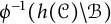 $\phi ^{-1}(h(\mathcal C)\setminus \mathcal B)$
for a homeomorphism
 $h\colon {\mathbb {P}}^2\setminus \mathcal B\to {\mathbb {P}}^2\setminus \mathcal B$
and a plane curve
 $\mathcal C\subset {\mathbb {P}}^2$
. However, it is not sure whether the branched cover
 $\phi $
is uniquely determined by
 $\theta $
. Hence, the splitting invariants do not contain any information of the ramification locus
 $\phi ^{-1}(\mathcal B)$
. The aim of this note is to give a generalization of splitting invariants including information near
 $\phi ^{-1}(\mathcal B)$
, called the G-combinatorial type (or the G-combinatorics for short). The idea is to investigate the boundary of a certain regular neighborhood of a plane curve, called the boundary manifold, based on arguments of graph manifolds [Reference Waldhausen38], plumbing graphs [Reference Neumann28], and modified plumbing graphs [Reference Hironaka20]. An obstruction to do this is that the plumbing graph naturally obtained from a plane curve (which corresponding to its combinatorics) may be non-normal in the sense of [Reference Neumann28]. In order to avoid this obstruction, we first discuss locally boundary manifolds near singularities of plane curves, and secondly consider the boundary manifold globally. As an application of G-combinatorics, we distinguish the embedded topology of quasi-triangular curves, which is a generalization of triangular curves studied in [Reference Artal Bartolo, Cogolludo-Agustín and Morales7] (Section 6). The embedded topology of quasi-triangular curves is not distinguished by splitting invariants.
In this note, we define a regular neighborhood
 $\mathcal {T}(\mathcal C)$
of a plane curve
 $\mathcal C$
as the algebraic neighborhood [Reference Durfee16], and we call its boundary
 $\mathscr {B}(\mathcal C):=\partial \mathcal {T}(\mathcal C)$
the boundary manifold of
 $\mathcal C$
(Section 3.2). We will obtain Theorem 1.2 below to prove the invariance of G-combinatorics in Section 3. Let
 $\mathcal C_1,\mathcal C_2\subset {\mathbb {P}}^2$
be two plane curves, and let
 $\sigma _i\colon Y_i\to {\mathbb {P}}^2$
be the minimal good embedded resolution of
 $\mathcal C_i$
. Put
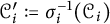 $\mathcal C_{i}':=\sigma _i^{-1}(\mathcal C_i)$
. Note that the combinatorics of
 $\mathcal C_i$
is redefined as the dual graph
 $ \mathrm {Cmb}(\mathcal C_i)$
of
 $\mathcal C_i'$
with marking
 $ \mathrm {Str}_{\mathcal C_i}$
of strict transforms of components of
 $\mathcal C_i$
in [Reference Artal Bartolo, Bannai, Shirane and Tokunaga3] (see Section 3.1 for details). We can define a meridian
 ${\mathfrak {m}_{D}}\in \pi _1({\mathbb {P}}^2\setminus \mathcal C_i)$
of each component
 $ D$
of
 $\mathcal C^{\prime }_{i}$
in
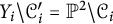 $Y_i\setminus \mathcal C_{i}'={\mathbb {P}}^2\setminus \mathcal C_i$
, which have canonically orientation derived from the complex structure of
 $Y_i$
(cf. [Reference Artal Bartolo, Cogolludo-Agustín and Tokunaga8, Definition 1.2] and [Reference Shirane35, p. 133]). We call
 $\mathfrak {m}_{D}^{-1}$
an anti-meridian of a component
 $ D$
of
 $\mathcal C_{i}'$
, which is a meridian with reversed orientation. It is known that a homeomorphism
 $h\colon U(\mathcal C_1)\rightarrow U(\mathcal C_2)$
induces an isomorphism
 $\Psi _h^\infty \colon \pi _1(\mathscr {B}(\mathcal C_1))\to \pi _1(\mathscr {B}(\mathcal C_2))$
. The following theorem follows from Theorem 3.10.
Theorem 1.2 Assume that there is a homeomorphism
 $h\colon U(\mathcal C_1)\rightarrow U(\mathcal C_2)$
with
 $h(\mathcal C_1)=\mathcal C_2$
for some regular neighborhoods
 $U(\mathcal C_i)$
. Then there exist an equivalence map
 $\varphi \colon \mathrm {Cmb}(\mathcal C_1)\to \mathrm { Cmb}(\mathcal C_2)$
and a homeomorphism
 $\Psi _{\mathscr {B}}\colon \mathscr {B}(\mathcal C_1)\to \mathscr {B}(\mathcal C_2)$
such that
-
(i)
$\Psi _{\mathscr {B}\ast }=\Psi _h^\infty $
; -
(ii) there is
$\alpha \in \{\pm 1\}$
such that
$\Psi _{\mathscr {B}\ast }(\mathfrak {m}_{D})=\mathfrak {m}_{\varphi (D)}^\alpha $
up to conjugate for any irreducible component
$ D$
of
$\mathcal C_1'$
, where
$ D$
is also regarded as a vertex of
$ \mathrm {Cmb}(\mathcal C_i)$
.





Let us state the main result of this note. Let G be a finite group. Assume that there are surjective homomorphisms
 $\theta _i\colon \pi _1({\mathbb {P}}^2\setminus \mathcal C_i)\to G$
. Then
 $\theta _i$
induce G-covers
 $\phi _i\colon X_i\to {\mathbb {P}}^2$
and
 $\tilde \phi _i\colon \widetilde {X}_i\to Y_i$
branched along sub-curves of
 $\mathcal C_i$
and
 $\mathcal C^{\prime }_{i}$
, respectively. Put
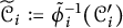 $\widetilde {\mathcal C}_{i}:=\tilde \phi _i^{-1}(\mathcal C^{\prime }_{i})$
. Since each irreducible component of
 $\widetilde {\mathcal C}_{i}$
is unibranched (cf. [Reference Laufer24, Chapter II]), we can define the dual graph
 $\Gamma _{i}^\theta $
of
 $\widetilde {\mathcal {C}}_{i}$
, and we will define a G-combinatorics
 $ \mathrm {Cmb}_G(\mathcal C_i,\theta _i)$
of
 $\mathcal C_i$
with respect to
 $\theta _i$
based on
 $\Gamma _i^\theta $
, which describes the topology of the boundary manifold of
 $\widetilde {\mathcal C}_{i}$
in
 $\widetilde {X}_i$
(Definition 4.2). For an equivalence map
 $\varphi \colon \mathrm {Cmb}(\mathcal C_1)\to \mathrm {Cmb}(\mathcal C_2)$
, we will define a G-equivalence map
 $\varphi _G^\theta \colon \mathrm {Cmb}_G(\mathcal C_1,\theta _1)\to \mathrm { Cmb}_G(\mathcal C_2,\theta _2)$
with respect to
 $\varphi $
(Definition 4.3). The following theorem follows from Theorem 4.4.
Theorem 1.3 Let
 $\mathcal C_i\subset {\mathbb {P}}^2$
be two plane curves with surjections
 $\theta _i\colon \pi _1({\mathbb {P}}^2\setminus \mathcal C_i)\to G$
. Assume that there are a homeomorphism
 $h\colon {\mathbb {P}}^2\to {\mathbb {P}}^2$
with
 $h(\mathcal C_1)=\mathcal C_2$
and an automorphism
 $\tau \colon G\to G$
such that
 $\tau \circ \theta _1=\theta _2\circ h_\ast $
, where
 $h_\ast \colon \pi _1({\mathbb {P}}^2\setminus \mathcal C_1)\to \pi _1({\mathbb {P}}^2\setminus \mathcal C_2)$
is the isomorphism induced by h. Let
 $\varphi \colon \mathrm {Cmb}(\mathcal C_1)\to \mathop {\mathrm {Cmb}}(\mathcal C_2)$
be the equivalence map induced by h. Then there is an equivalence map
 $\varphi _G^\theta \colon \mathrm {Cmb}_G(\mathcal C_1,\theta _1)\to \mathrm { Cmb}_G(\mathcal C_2,\theta _2)$
with respect to
 $\varphi $
.
Remark 1.4 The G-combinatorics
 $ \mathrm {Cmb}_G(\mathcal C_i,\theta _i)$
of
 $\mathcal C_i\subset {\mathbb {P}}^2$
with respect to
 $\theta _i\colon \pi _1({\mathbb {P}}^2\setminus \mathcal C_i)\to G$
can be algebraically constructed from the minimal resolution
 $\tilde {\sigma }^{\prime }_{i}\colon \widetilde {X}^{\prime }_{i}\to \widetilde {X}_i$
of the G-cover
 $\tilde \phi _i\colon \widetilde {X}_i\to Y_i$
and the pull-back
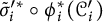 ${\tilde {\sigma }_i^{\prime \ast }}\circ \phi _i^\ast (\mathcal C^{\prime }_{i})$
, and describe the topology of the boundary manifold of
 $\tilde \phi _i^{-1}(\mathcal C^{\prime }_{i})$
in
 $\widetilde {X}_i$
(cf. Remark 4.1). Hence, it may be good to compare some topological invariant (like the linking invariant) and some algebraic data (like splitting invariants) through G-combinatorics. In fact, known splitting invariants can be constructed from G-combinatorics (see Section 5).
This note is organized as follows: In Section 2, we recall the definitions of graph manifolds, plumbing graphs, and modified plumbing graphs, and several results in [Reference Waldhausen38], [Reference Neumann28]. In Section 3, we give proofs of Fact 1.1 and Theorem 1.2 by using arguments of [Reference Neumann28, Reference Waldhausen38]. In Section 4, we define the G-combinatorics based on the results in [Reference Hironaka20] and prove Theorem 1.3. In Section 5, we construct known splitting invariants from the G-combinatorics. In Section 6, we distinguish the embedded topology of quasi-triangular curves by G-combinatorics. In the Appendix, we recall results of [Reference Neumann28, Reference Waldhausen38] and several papers, which we use in this note.
2 Preliminary
We call a manifold of real dimension n an n-manifold. For a compact manifold M and a union F of closed subspaces of M, we choose a (finite) triangulation, in which each component of F is a subcomplex. The closed star of F in the second barycentric subdivision for the triangulation of M is called a regular neighborhood of F in M, denoted by
 $U_M(F)$
. If there is no confusion,
 $U_M(F)$
is simply denoted as
 $U(F)$
. We may assume that a regular neighborhood is sufficiently small. For a subset
 $A\subset M$
, let
 $A^\circ $
denote the interior of A in M.
In this note, a graph
 $\Gamma $
means a collection of vertices
 $\mathcal {V}(\Gamma )$
and oriented edges
 $\mathcal {Y}(\Gamma )$
together with maps
 $$ \begin{align*} o&\colon \mathcal{Y}(\Gamma)\longrightarrow \mathcal{V}(\Gamma), & t&\colon \mathcal{Y}(\Gamma)\longrightarrow \mathcal{V}(\Gamma), & \bar{\ \ }&\colon \mathcal{Y}(\Gamma) \longrightarrow \mathcal{Y}(\Gamma) \quad (y\longmapsto \overline{y}) \end{align*} $$
satisfying
 $o(\overline {y})=t(y)$
,
 $t(\overline {y})=o(y)$
,
 $\overline {y}\ne y,$
and
 $\overline {\overline {y}}=y$
. For each
 $y\in \mathcal {Y}(\Gamma )$
, we call
 $o(y)$
the initial vertex,
 $t(y)$
the terminal vertex, and
 $\overline {y}$
the inverse edge of y. In a figure of a graph
 $\Gamma $
, we depict the set
 $\{y,\overline {y}\}$
as a segment from
 $o(y)$
to
 $t(y)$
for each edge
 $y\in \mathcal {Y}(\Gamma )$
. Let
 $ \boldsymbol {d}\colon \mathcal {V}(\Gamma )\to \mathbb Z_{\geq 0} $
be the degree map, that is,
 $\boldsymbol {d}(v)$
is the number of edges
 $y\in \mathcal {Y}(\Gamma )$
with
 $t(y)=v$
for each
 $v\in \mathcal {V}(\Gamma )$
.
Throughout this note, we put
 $$ \begin{align*} I&:=[0,1]\subset{\mathbb{R}}, & { \mathbb{D}^2}&:=\{z\in\mathbb C\mid |z|\leq 1\}, & S^1&:=\{z\in \mathbb C\mid |z|=1\}. \end{align*} $$
For
 $A=(\begin {smallmatrix} a&b\\c&d \end {smallmatrix}) \in \mathrm {SL}(2,\mathbb Z)$
, A also denotes the diffeomorphism
 $T\to T$
of the torus
 $T:=S^1\times S^1$
given by
 $A(t_1, t_2):=(t_1^at_2^b, t_1^ct_2^d)$
. Throughout this note, we assume that the total space M of an
 $S^1$
-bundle
 $p\colon M\to B$
is orientable (the base space B may be non-orientable).
Let B be a (compact)
 $2$
-manifold of genus g with d boundary components
 $\partial B_1,\dots , \partial B_d\cong S^1$
, with the convention that
 $g<0$
if B is non-orientable. Let
 $p\colon M\to B$
be an
 $S^1$
-bundle. For a boundary component
 $\partial M_i:=p^{-1}(\partial B_i)$
of M, an orientation preserving homeomorphism
 $\tau _i\colon S^1\times S^1\to \partial M_i$
is called a trivialization of
 $\partial M_i$
if
 $p\circ \tau _i$
is a projection to either the first or second component of
 $S^1\times S^1$
. Unless otherwise noted, we assume that
 $p\circ \tau _i$
is the projection to the first component:
 $$\begin{align*}p\circ \tau_i(t_1,t_2)= t_1\in S^1\cong \partial { B_i}. \end{align*}$$
For an
 $S^1$
-bundle
 $p\colon M\to B$
, we fix a trivialization for each boundary component of M. Then the Euler number e of the
 $S^1$
-bundle p is the cross-section obstruction (cf. [Reference Hirzebruch, Neumann and Koh22, p. 59]). In [Reference Waldhausen38], several properties of
 $S^1$
-bundles over
 $2$
-manifolds are proved. In Appendix A, results which we need in this note are stated.
2.1 Graph manifolds
We recall graph manifolds, which are defined and classified (with minor exceptions) by Waldhausen [Reference Waldhausen38]. In particular, we state several facts for graph manifolds with boundary. (In [Reference Waldhausen38], the same facts are proved for graph manifolds without boundary except for several cases.)
Let M be a
 $3$
-manifold, and let
 $\mathbb T:=T_1\cup \dots \cup T_n\subset M^\circ $
(
 $n\geq 0$
) be a disjoint union of tori. Let
 $U(\mathbb T)$
be a regular neighborhood of
 $\mathbb T$
in M. We call
 $\mathbb T$
a graph structure for M if every connected component of
 $M\setminus U(\mathbb T)^\circ $
is homeomorphic to an
 $S^1$
-bundle over
 $2$
-manifolds. A
 $3$
-manifold with a graph structure is called a graph manifold.
A graph structure
 $\mathbb T$
of a
 $3$
-manifold M is said to be reduced if it does not satisfy any of the ten conditions in [Reference Waldhausen38, Definition 6.2]. We omit to state the ten conditions, but that
 $M\setminus U(\mathbb T)^\circ $
has no component homeomorphic to
 $I\times S^1\times S^1$
. A
 $3$
-manifold with a fixed reduced graph structure is called a reduced graph manifold. For reduced graph manifolds with boundary, Waldhausen proved the following theorem.
Theorem 2.1 (cf. [Reference Waldhausen38, Theorem 8.1])
For each
 $i=1,2$
, let
 $M_i$
be a reduced graph manifold with boundary and a graph structure
 $\mathbb T_i$
. If there is a homeomorphism
 $h\colon M_1\to M_2$
, then there is an isotopy
 $\mathfrak {h}_u\colon M_1\to M_2 (0\leq u\leq 1)$
such that
 $\mathfrak {h}_0=h$
and
 $\mathfrak {h}_1(\mathbb T_1)=\mathbb T_2$
.
For a reduced graph manifold M, Waldhausen defined a weighted graph
 $\Gamma _{\mathrm {W}}(M)$
, which is called W-graph in [Reference Neumann28], and proved Theorem 2.2 below. The W-graph
 $\Gamma _{\mathrm {W}}(M)$
consists of the following data:
-
• there is a bijection from
$\mathcal {V}(\Gamma _{\mathrm {W}}(M))$
to the set of connected components of
$M\setminus U(\mathbb T)^\circ $
, and let
$M_v$
be the component corresponding to the vertex v for each
$v\in \mathcal {V}(\Gamma _{\mathrm {W}}(M))$
; -
• if
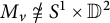
$M_v\not \cong S^1\times { \mathbb {D}^2}$
for
$v\in \mathcal {V}(\Gamma _{\mathrm {W}}(M))$
,
$M_v$
has the unique
$S^1$
-bundle structure
$p_v\colon M_v\to B_v$
up to isotopy by Theorem A.6, and v is assigned a triple of integers
$(g_v,r_v,s_v),$
where
$g_v$
is the genus of
$B_v$
,
$r_v$
is the number of boundary components of M contained in
$M_v$
, and
$s_v$
is the Euler number of
$p_v\colon M_v\to B_v$
if
$r_v=0$
,
$s_v$
vanishes if
$r_v>0$
; -
• each
$v\in \mathcal {V}(\Gamma _{\mathrm {W}}(M))$
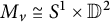
with
$M_v\cong S^1\times {\mathbb {D}^2}$
is left unweighted; -
• there is a bijection from
$\mathcal {Y}(\Gamma _{\mathrm {W}}(M))$
to the set of components of
$\partial U(\mathbb T)$
, write
$y\mapsto T_y\subset \partial U(\mathbb T)$
for each
$y\in \mathcal {Y}(\Gamma _{\mathrm {W}}(M))$
, satisfying-
–
$T_y\subset M_{t(y)}$
for each
$y\in \mathcal {Y}(\Gamma _{\mathrm {W}}(M))$
; -
– for each
$T\subset \mathbb T$
, there is
$y\in \mathcal {Y}(\Gamma _{\mathrm {W}}(M))$
such that
$\partial U(T)=T_y\cup T_{\overline {y}}$
(note that M can be regarded as the manifold given by gluing
$M_{t(y)}$
and
$M_{t(\overline {y})}$
via certain homeomorphisms
$T_y\to T_{\overline {y}}$
for
$y\in \mathcal {Y}(\Gamma _{\mathrm {W}}(M))$
since
$U(T)\cong I\times S^1\times S^1$
for each component
$T\subset \mathbb T$
); -
-
• each
$y\in \mathcal {Y}(\Gamma _{\mathrm {W}}(M))$
is assigned a pair
$(\alpha _y,\beta _y)$
of integers satisfying and
$$ \begin{align*} &\gcd(\alpha_y,\beta_y)=1, \qquad 0\leq\beta_y<\alpha_y, \qquad \alpha_{\overline{y}}=\alpha_{y}, \qquad \beta_{\overline{y}}\beta_y\equiv 1 \pmod{\alpha_y} \end{align*} $$
$\beta _y>0$
if y is adjacent to an unweighted vertex, which is uniquely determined by the pasting of
$M_{o(y)}$
and
$M_{t(y)}$
at
$T_y$
;
-
• each edge
$y\in \mathcal {Y}(\Gamma _{\mathrm {W}}(M))$
is assigned a sign
$\varepsilon _y\in \{\pm 1\}$
, which depends on orientations of fibers of
$M_{o(y)}$
and
$M_{t(y)}$
. Let
$\Gamma _{\mathrm {W}}^\ast (M)$
be the full subgraph of
$\Gamma _{\mathrm {W}}(M)$
given by removing
$v\in \mathcal {V}(\Gamma _{\mathrm {W}}(M))$
with
$g_v<0$
. Then
$\Gamma _{\mathrm {W}}(M)$
is assigned the map
$\varepsilon _M\colon H_1(\Gamma _{\mathrm {W}}^\ast (M))\to \mathbb Z/2\mathbb Z$
defined by
$\varepsilon _M(C)$
equal to the number modulo
$2$
of
$y\in \mathcal {Y}(C)$
with
$\varepsilon _y=-1$
for any cycle C of
$\Gamma _{\mathrm {W}}^\ast (M)$
, which is uniquely determined.







































Moreover, the equivalence of W-graphs is also defined in [Reference Waldhausen38]. Under our notation of graphs, for reduced graph manifolds
 $M_i$
with boundary, W-graphs
 $\Gamma _{\mathrm {W}}(M_1)$
and
 $\Gamma _{\mathrm {W}}(M_2)$
are equivalent if they satisfy one of the following conditions:
-
• there is an isomorphism
$\varphi \colon \Gamma _{\mathrm {W}}(M_1)\to \Gamma _{\mathrm {W}}(M_2)$
of graphs preserving weights
$(g_v,r_v,s_v)$
of
$v\in \mathcal {V}(\Gamma _{\mathrm {W}}(M_1))$
and
$(\alpha _y,\beta _y)$
of
$y\in \mathcal {Y}(\Gamma _{\mathrm {W}}(M_1))$
, and
$\varphi $
is compatible with
$\varepsilon _{M_i}\colon H_1(\Gamma _{\mathrm {W}}^\ast (M_i))\to \mathbb Z/2\mathbb Z$
, that is,
$\varepsilon _{M_1}=\varepsilon _{M_2}\circ \varphi _\ast $
; -
• the pair of
$\Gamma _{\mathrm {W}}(M_1)$
and
$\Gamma _{\mathrm {W}}(M_2)$
is that of the following graphs: (2.1)










We call the isomorphism
 $\varphi \colon \Gamma _{\mathrm {W}}(M_1)\to \Gamma _{\mathrm {W}}(M_2)$
above an equivalence map of W-graphs. The proof of [Reference Waldhausen38, Theorem 9.4] shows the following theorem.
Theorem 2.2 (cf. [Reference Waldhausen38, Theorem 9.4])
Let
 $M_i$
,
 $i=1,2$
, be two oriented reduced graph manifolds with boundary and reduced graph structure
 $\mathbb T_i$
. Then
 $M_1$
and
 $M_2$
are orientation-preserving homeomorphic if and only if the W-graphs
 $\Gamma _{\mathrm {W}}(M_1)$
and
 $\Gamma _{\mathrm {W}}(M_2)$
are equivalent.
Moreover, if
 $h\colon M_1\to M_2$
is an orientation preserving homeomorphism, and the pair of
 $\Gamma _{\mathrm {W}}(M_i)$
is not that of (2.1), then there is an isotopy
 $\mathfrak {h}_u\colon M_1\to M_2 (0\leq u\leq 1)$
such that
 $\mathfrak {h}_0=h$
and
 $\mathfrak {h}_1$
satisfies the following conditions:
-
(i)
$\mathfrak {h}_1(\mathbb T_1)=\mathbb T_2$
; -
(ii)
$\mathfrak {h}_1$
induces an equivalence map
$\varphi \colon \Gamma _{\mathrm {W}}(M_1)\to \Gamma _{\mathrm {W}}(M_2)$
of W-graphs such that
$\mathfrak {h}_1(M_{1,v})=M_{2,\varphi (v)}$
for each
$v\in \mathcal {V}(\Gamma _{\mathrm {W}}(M_1))$
, where
$M_{i,v_i}$
is the component of
$M_i\setminus U(\mathbb T_i)^\circ $
corresponding to
$v_i\in \mathcal {V}(\Gamma _{\mathrm {W}}(M_i))$
; -
(iii)
$\mathfrak {h}_1$
maps every fiber of the
$S^1$
-bundle
$p_{1,v}\colon M_{1,v}\to B_{1,v}$
to that of
$p_{2,\varphi (v)}\colon M_{2,\varphi (v)}\to B_{2,\varphi (v)}$
if
$M_{1,v}\not \cong { \mathbb {D}^2}\times S^1$
for
$v\in \mathcal {V}(\Gamma _{\mathrm {W}}(M_1))$
.














2.2 Plumbing graphs
Neumann [Reference Neumann28] defined plumbed 3-manifolds corresponding to plumbing graphs based on Waldhausen’s work [Reference Waldhausen38]. In the appendix of [Reference Neumann28], he also defined decorated plumbing graphs to describe boundary framed graph manifolds, which are graph manifolds with fixed trivialization of each boundary component. In this note, we associate a decorated plumbing graph with the graph manifold constructed from the induced plumbing graph as mentioned in [Reference Neumann28, p. 339], which is called the plumbed manifold. We recall the (connected) decorated plumbing graph and such a graph manifold.
A decorated plumbing graph
 $\Gamma _{\mathrm {dpg}}=(\Gamma , \boldsymbol {g}, \boldsymbol {e}, \mathrm {sgn}; \overline {\mathcal {A}},\mathcal {A})$
is a finite connected graph
 $\Gamma $
together with a partition
 $\mathcal {V}(\Gamma )=\overline {\mathcal {A}}(\Gamma )\sqcup \mathcal {A}(\Gamma )$
such that
 $\boldsymbol {d}(v)\leq 1$
for each
 $v\in \mathcal {A}(\Gamma )$
, and maps
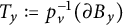
 $$ \begin{align*} \boldsymbol{g} &\colon \overline{\mathcal{A}}(\Gamma) \longrightarrow \mathbb Z, & \boldsymbol{e} &\colon \overline{\mathcal{A}}(\Gamma) \longrightarrow \mathbb Z, & \mathrm{sgn} &\colon \mathcal{Y}(\Gamma) \longrightarrow \{\pm1\} \end{align*} $$
satisfying
 $\mathrm {sgn}(y)=\mathrm {sgn}(\overline {y})$
for any
 $y\in \mathcal {Y}(\Gamma )$
. A vertex in
 $\mathcal {A}(\Gamma )$
is called a boundary vertex, and drawn in the graph as an arrow head
 . An edge
 $y\in \mathcal {Y}(\Gamma )$
is called a
 $(+)$
-edge if
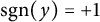 $\mathrm {sgn}(y)=+1$
, and a
 $(-)$
-edge otherwise. In the case where
 $\mathcal {A}(\Gamma )=\emptyset $
,
 $\Gamma _{\mathrm {dpg}}$
is a plumbing graph, and we denote it by
 $\Gamma _{\mathrm {pg}}=(\Gamma ,\boldsymbol {g}, \boldsymbol {e}, \mathrm {sgn})$
.
Let
 $\Gamma _{\mathrm {dpg}}=(\Gamma ,\boldsymbol {g},\boldsymbol {e}, \mathrm {sgn}; \overline {\mathcal {A}}, \mathcal {A})$
be a decorated plumbing graph with
 $\overline {\mathcal {A}}(\Gamma )\ne \emptyset $
. The plumbed manifold
 $\mathscr {P}(\Gamma _{\mathrm {dpg}})$
for
 $\Gamma _{\mathrm {dpg}}$
is the graph manifold constructed as follows:
-
(I) For
$v\in \overline {\mathcal {A}}(\Gamma )$
, let
$B_v$
be a compact
$2$
-manifold of genus
$\boldsymbol {g}(v)$
with
$\boldsymbol {d}(v)$
boundary components
$\partial B_{y}$
, labeled by edges
$y\in \mathcal {Y}(\Gamma )$
with
$t(y)=v$
; and let
$p_v\colon M_v\to B_v$
be an
$S^1$
-bundle, where, for each
$y\in \mathcal {Y}(\Gamma )$
with
$t(y)=v$
, the boundary component
$T_{y}:=p_{v}^{-1}(\partial B_y)$
of
$M_{v}$
has a fixed trivialization
$ \tau _y\colon S^1\times S^1\to T_y $
such that the Euler number of
$p_v$
is
$\boldsymbol {e}(v)$
. -
(II) The plumbed manifold
$\mathscr {P}(\Gamma _{\mathrm {dpg}})$
is constructed by gluing
$M_{t(y)}$
and
$M_{t(\overline {y})}$
at
$T_y\subset M_{t(y)}$
and
$T_{\overline {y}}\subset M_{t(\overline {y})}$
by the homeomorphism (2.2)for each
$$ \begin{align} T_{\overline{y}}\xrightarrow{\ \tau_{\overline{y}\ }^{-1}} S^1\times S^1 \xrightarrow{\mathrm{sgn}(y) J} S^1\times S^1\xrightarrow{\ \tau_y\ } T_y \end{align} $$
$y\in \mathcal {Y}$
with
$o(y),t(y)\in \overline {\mathcal {A}}(\Gamma )$
, where
$J:=(\begin {smallmatrix} 0&1\\1&0 \end {smallmatrix})$
.











For
 $v\in \overline {\mathcal {A}}(\Gamma )$
, we call
 $p_v\colon M_v\to B_v$
(or
 $M_v$
) the
 $S^1$
-bundle of v,
 $B_v$
the base 2-manifold of v, and a fiber of
 $p_v$
a fiber of v. An edge
 $y\in \mathcal {Y}(\Gamma )$
with
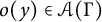 $o(y)\in \mathcal {A}(\Gamma )$
corresponds to a boundary component
 $T_y$
of
 $\mathscr {P}(\Gamma _{\mathrm {dpg}})$
. Since the gluing maps reverse orientation,
 $\mathscr {P}(\Gamma _{\mathrm {dpg}})$
inherits compatible orientations from all pieces
 $M_v$
. The number of boundary components of
 $\mathscr {P}(\Gamma _{\mathrm {dpg}})$
is equal to
 $\#\mathcal {A}(\Gamma )$
. By abuse of notation, let
 $T_y$
denote the resulting torus in
 $\mathscr {P}(\Gamma _{\mathrm {dpg}})$
by gluing
 $T_y\subset M_{t(y)}$
and
 $T_{\overline {y}}\subset M_{t(\overline {y})}$
, hence
 $T_y=T_{\overline {y}}$
in
 $\mathscr {P}(\Gamma _{\mathrm {dpg}})$
.
In this note, we consider
 $\mathscr {P}(\Gamma _{\mathrm {dpg}})$
as a closed submanifold of a graph manifold M. An edge
 $y\in \mathcal {Y}(\Gamma )$
with
 $t(y)\in \mathcal {A}(\Gamma )$
corresponds to the boundary component
 $T_y$
of
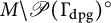 $M\setminus \mathscr {P}(\Gamma _{\mathrm {dpg}})^\circ $
which is identified with
 $T_{\overline {y}}\subset M_{o(t)}\subset \mathscr {P}(\Gamma )$
in M, and
 $t(y)\in \mathcal {A}(\Gamma )$
corresponds to an
 $S^1$
-bundle part
 $M_{t(y)}$
of
 $M\setminus \mathscr {P}(\Gamma )^\circ $
such that
 $T_y\subset M_{t(y)}$
.
Remark 2.3 Here, we do not give the definition of plumbing graph introduced in [Reference Neumann28]. Plumbed manifolds having boundary without trivialization are considered by using the plumbing graphs in [Reference Neumann28]. In [Reference Neumann28, p. 339], it is mentioned that each boundary vertex
 $v\in \mathcal {A}(\Gamma )$
of a decorated plumbing graph
 $\Gamma _{\mathrm {dpg}}$
can be regarded as a vertex v of a plumbing graph with weights
 $\boldsymbol {g}(v)=0$
,
 $\boldsymbol {e}(v)=0$
and
 $r_v=1$
, where
 $r_v$
is the number of “free” boundary components of the
 $S^1$
-bundle
 $M^{\prime }_v$
, that is,
 $v\in \mathcal {A}(\Gamma )$
corresponds to
 $M_v'\cong I\times S^1\times S^1$
one of whose boundary components does not have trivialization. In this note, we can regard such
 $M_v'$
as a submanifold of the above
 $S^1$
-bundle part
 $M_v\subset M\setminus \mathscr {P}(\Gamma )^\circ$
.
Remark 2.4 For the aim of this note, it is enough to consider decorated plumbing graphs with
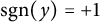 $\mathrm {sgn}(y)=+1$
for any
 $y\in \mathcal {Y}(\Gamma )$
in many cases. If we assume that
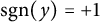 $\mathrm {sgn}(y)=+1$
for each
 $y\in \mathcal {Y}(\Gamma )$
, then, by omitting the map
 $\mathrm {sgn}\colon \mathcal {Y}(\Gamma )\to \{\pm 1\}$
, we write
 $\Gamma _{\mathrm {dpg}}=(\Gamma , \boldsymbol {g}, \boldsymbol {e}; \overline {\mathcal {A}}, \mathcal {A})$
or
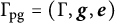 $\Gamma _{\mathrm {pg}}=(\Gamma ,\boldsymbol {g},\boldsymbol {e})$
if
 $\mathcal {A}(\Gamma )=\emptyset $
.
Notation. We follow [Reference Neumann28, Appendix] to describe a decorated plumbing graph. Namely, a vertex
 $v\in \mathcal {V}(\Gamma )$
is written as follows:

We omit the weight of
 $\{y,\overline {y}\}$
if
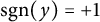 $\mathrm {sgn}(y)=+1$
, and we write
 $-$
if
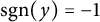 $\mathrm {sgn}(y)=-1$
. If
 $\boldsymbol {g}(v)=0$
, we may omit it. For example, the left decorated plumbing graph is “shorthand” for the right plumbing graph in the following graphs:

A chain of length k in
 $\Gamma _{\mathrm {dpg}}$
is any part
 $\mathfrak {c}$
of
 $\Gamma _{\mathrm {dpg}}$
of the following form with arbitrary edge signs (after relabeling vertices):

say
 $v_i$
the vertex on the above parts with
 $\boldsymbol {e}(v_i)=e_i$
. The chain
 $\mathfrak {c}$
above is said to be incident to a boundary vertex if either
 $v_1$
or
 $v_k$
is adjacent to a boundary vertex. An edge
 $y\in \mathcal {Y}(\Gamma )$
is regarded as a chain of length
 $0$
. A chain is maximal if it can be included in no larger chain.
In [Reference Neumann28, Proposition 2.1], nine operations (R0)–(R8) and their inverses to plumbing graphs are given, which do not change the diffeomorphism type of their plumbed
 $3$
-manifolds (hence also homeomorphism type). In [Reference Neumann28, Appendix], (R0)–(R7) are modified to F-calculus for applying decorated plumbing graphs ((R8) is removed). Moreover, the F-normal forms of decorated plumbing graphs are defined, which any decorated plumbing graph can be reduced to F-normal form using only F-calculus and their inverses.
Remark 2.5 In this article, we use the following five of F-calculus to obtain F-normal forms:

where
 $g\#(-1):=-2g-1$
if
 $g\geq 0$
, and
 $g\#(-1):=g-1$
otherwise. In [Reference Neumann28], the operations (
 $\mathrm {R1}_0^+$
), (
 ${\mathrm {R1}}^+$
), (
 ${\mathrm {R1}}^-$
), and (
 ${\mathrm {R1}}^{++}$
) are called blowing-downs and their reverse are called blowing-ups, and (R2) is called an
 ${\mathbb {R}}{\mathbb {R}}{\mathbb {P}}^2$
-absorption and its reverse is called an
 ${\mathbb {R}}{\mathbb {P}}^2$
-extrusion. Note that the blowing-down (
 $\mathrm {R1}^{++}$
) is different from the blowing-down of the dual graph for an algebraic curve on a complex surface.
Remark 2.6 For a decorated plumbing graph
 $\Gamma _{\mathrm {dpg}}=(\Gamma ,\boldsymbol {g},\boldsymbol {e},\mathrm {sgn};\overline {\mathcal {A}}, \mathcal {A})$
, let
 $\Gamma ^{\ast }$
be the full subgraph of
 $\Gamma $
defined by all vertices
 $v\in \overline {\mathcal {A}}(\Gamma )$
with
 $\boldsymbol {g}(v)\geq 0$
and all boundary vertices in
 $\mathcal {A}(\Gamma )$
. As mentioned in [Reference Neumann28, p. 340], the information contained in the edge weights is completely coded up to the F-calculus corresponding to (R0) in [Reference Neumann28, Proposition 2.1] by a homomorphism
 $\varepsilon _{\Gamma _{\mathrm {dpg}}}\colon H_1(\Gamma ^{\ast },\mathcal {A}(\Gamma ))\to \mathbb Z/2\mathbb Z$
which assigns to any relative cycle C of
 $(\Gamma ^{\ast },\mathcal {A}(\Gamma ))$
the number modulo
 $2$
of
 $(-)$
-edges on C.
Definition 2.7 Let
 $\Gamma _{\mathrm {dpg}}=(\Gamma ,\boldsymbol {g},\boldsymbol {e};\overline {\mathcal {A}}, \mathcal {A})$
be a decorated plumbing graph with
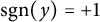 $\mathrm {sgn}(y)=+1$
for each
 $y\in \mathcal {Y}(\Gamma )$
. The intersection form
 $S(\Gamma _{\mathrm {dpg}})$
of
 $\Gamma _{\mathrm {dpg}}$
can be defined as in [Reference Neumann28, Section 8]. Namely, if
 $\overline {\mathcal {A}}(\Gamma )=\{v_1,\dots ,v_r\}$
, then
 $S(\Gamma _{\mathrm {dpg}}):=(a_{ij})_{i,j=1,\dots ,r}$
with
 $$ \begin{align*} a_{ij}:=\left\{\begin{array}{@{}ll} \boldsymbol{e}(v_i) + \#\{y\in\mathcal{Y}(\Gamma)\mid o(y)=t(y)=v_i\} & (i=j), \\[0.3em] \#\{ y\in\mathcal{Y}(\Gamma) \mid o(y)=v_i, t(y)=v_j \} & (i\ne j). \end{array}\right. \end{align*} $$
In Appendix B, we recall properties of plumbing graphs which are used in this note.
2.3 Modified plumbing graphs
Hironaka [Reference Hironaka20] defined modified plumbing graphs to describe normal surface–curve pairs
 $(X,\mathcal C)$
which are pairs of a complex normal surface X and an algebraic curve
 $\mathcal C\subset X$
. We will use modified plumbing graph to define a G-combinatorics for a plane curve. In this section, we recall the definition of the modified plumbing graph without boundary vertices.
Let
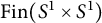 $\mathrm {Fin}(S^1\times S^1)$
be the set of finite unbranched coverings from
 $S^1\times S^1$
to itself. A modified plumbing graph
 $\Gamma _{\mathrm {pg}}^{\mathrm {m}}=(\Gamma , \boldsymbol {g}, \boldsymbol {e}, \boldsymbol {m})$
is a plumbing graph
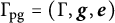 $\Gamma _{\mathrm {pg}}=(\Gamma ,\boldsymbol {g},\boldsymbol {e})$
satisfying
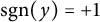 $\mathrm {sgn}(y)=+1$
for each
 $y\in \mathcal {Y}(\Gamma )$
together with a map
 $\boldsymbol {m}\colon \mathcal {Y}(\Gamma ) \to \mathrm {Fin}(S^1\times S^1)$
such that
-
(i) by choosing certain bases of tori
$S^1\times S^1$
, the unbranched coverings
$\boldsymbol {m}(y)\colon S^1\times S^1\to S^1\times S^1$
are represented by matrices in
$M_2(\mathbb Z)$
of the following form: (2.3)where
$$ \begin{align} \boldsymbol{m}(y)=\begin{pmatrix} c(y) & 0 \\ b(y) & a(y) \end{pmatrix}\colon S^1\times S^1\longrightarrow S^1\times S^1, \end{align} $$
$0\leq b(y)<a(y)$
and
$c(y)>0$
;
-
(ii) the induced maps
$\boldsymbol {m}(y)_\ast $
and
$(J\,\boldsymbol {m}(\overline {y}))_\ast $
from
$\pi _1(S^1\times S^1)$
to
$\pi _1(S^1\times S^1)$
have the same image in
$\pi _1(S^1\times S^1)\cong \mathbb Z\oplus \mathbb Z$
.








Remark 2.8 The above definition of
 $\boldsymbol {m}(y)$
is different from
 $m(y)$
in [Reference Hironaka20]. This difference comes from the difference of trivializations for boundary components of
 $S^1$
-bundles as follows: For an
 $S^1$
-bundle
 $p\colon M\to B$
over a
 $2$
-manifold B with boundary, each boundary
 $T_i\subset \partial M$
is trivialized by a homeomorphism
 $\tau _i\colon S^1\times S^1\to T_i$
such that
 $p\circ \tau _i$
is the projection onto the second component in [Reference Hironaka20], but onto the first one in this note according to [Reference Neumann28], that is,
 $\boldsymbol {m}(y)=Jm(y)J$
. Hence,
 $a(y), b(y),$
and
 $c(y)$
in this note play the same role of those in [Reference Hironaka20].
Given a modified plumbing graph
 $\Gamma _{\mathrm {pg}}^{\mathrm {m}}=(\Gamma ,\boldsymbol {g},\boldsymbol {e},\boldsymbol {m})$
, an associated graph manifold
 $\mathscr {P}(\Gamma _{\mathrm {pg}}^{\mathrm {m}})$
is defined as follows: For each
 $v\in \mathcal {V}(\Gamma )$
, let
 $B_v$
be a compact
 $2$
-manifold of genus
 $\boldsymbol {g}(v)$
with boundary components, labeled by
 $y\in \mathcal {Y}(\Gamma )$
with
 $t(y)=v$
, and let
 $p_v\colon M_v\to B_v$
be an
 $S^1$
-bundle, where
 $M_v$
is an oriented
 $3$
-manifold with trivializations at boundary components such that the Euler number of
 $p_v$
is
 $\boldsymbol {e}(v)$
. For each
 $y\in \mathcal {Y}(\Gamma )$
, let
 $T_y\subset M_{t(y)}$
be the boundary component associated with y with trivialization
 $\tau _y\colon S^1\times S^1\to T_y$
, and put
 $R_y:=\boldsymbol {m}(y)^{-1} J \boldsymbol {m}(\overline {y})$
. By condition (ii) of
 $\boldsymbol {m}$
, we have
 $R_y\in \mathrm {GL}(2,\mathbb Z)$
,
 $\det R_y=-1$
, and
 $R_y$
represent homeomorphisms
 $T_{\overline {y}}\to T_y$
:

The manifold
 $\mathscr {P}(\Gamma _{\mathrm {pg}}^{\mathrm {m}})$
is obtained by gluing
 $M_{t(y)}$
and
 $M_{t(\overline {y})}$
by
 $R_y$
.
Remark 2.9 For
 $y\in \mathcal {Y}(\Gamma )$
,
 $\boldsymbol {m}(y)\colon S^1\times S^1\to S^1\times S^1$
coincides with the map induced by the map
 $$\begin{align*}\mathbb C^2\setminus\{u_1v_1\ne0\}\ni (u_1,v_1)\longmapsto(u_1^{c(y)},u_1^{b(y)}v_1^{a(y)})=(u_2,v_2)\in\mathbb C^2\setminus\{u_2v_2\ne0\}\end{align*}$$
by regarding
 $S^1\times S^1$
as
 $\{|u_i|=|v_i|=1\}$
. This map appears in [Reference Laufer24, Chapter 2] to construct a resolution of singularities of two-dimensional analytic spaces. Note that the dual graph of the exceptional divisor on the resolution is a chain, and
 $\mathscr {P}(\Gamma _{\mathrm {pg}}^{\mathrm {m}})$
can be constructed as the plumbed manifold
 $\mathscr {P}(\Gamma _{\mathrm {pg}})$
of
 $\Gamma _{\mathrm {pg}}$
, where
 $\Gamma _{\mathrm {pg}}$
is the plumbing graph constructed by replacing each edge of
 $\Gamma _{\mathrm {pg}}^{\mathrm {m}}$
with the chain of the exceptional divisor. By the resolution in [Reference Laufer24], we can check that the basis of
 $H_1(T_y,\mathbb Z)$
giving the matrix (2.3) corresponding to the basis given by
 $\Gamma _{\mathrm {pg}}$
.
3 Combinatorial type of plane curves
In this section, we prove Fact 1.1 and Theorem 1.2. We first recall the combinatorial type of a plane curve. The combinatorial type is defined in [Reference Artal Bartolo, Cogolludo-Agustín and Tokunaga8] as the data consisting of the number of irreducible components, the degrees and singularities of irreducible components, and configuration of components. In [Reference Artal Bartolo, Bannai, Shirane and Tokunaga3], it is redefined by using the resolution graph of plane curves, which we explain below.
3.1 Combinatorial type
Let
 $\mathcal C\subset {\mathbb {P}}^2$
be a plane curve of degree d, and let
 $\mathrm {Irr}(\mathcal C)$
denote the set of irreducible components of
 $\mathcal C$
. Let
 $\sigma \colon Y\to {\mathbb {P}}^2$
be the minimal good embedded resolution of the singularities
 $ \mathrm {Sing}(\mathcal C)$
of
 $\mathcal C$
, that is, the minimal sequence of blowing-ups which resolves
 $\mathop {\mathrm {Sing}}(\mathcal C)$
and such that
 $\sigma ^{-1}(\mathcal C)$
is a simple normal crossing divisor. Put
 $$\begin{align*}{\mathcal C'}:=\sigma^{-1}(\mathcal C). \end{align*}$$
In [Reference Artal Bartolo, Bannai, Shirane and Tokunaga3], the combinatorial type (or the combinatorics for short)
 $ \mathrm { Cmb}(\mathcal C)$
of the plane curve
 $\mathcal C$
is redefined as the
 $3$
-tuple
 $ \mathrm {Cmb}(\mathcal C):=(\Gamma _{\mathcal C}, \mathrm {Str}_{\mathcal C}, \boldsymbol {e}_{\mathcal C})$
, where
-
•
$\Gamma _{\mathcal C}$
is the dual graph of
$ \mathcal C'$
, -
•
$ \mathrm {Str}_{\mathcal C}\subset \mathcal {V}(\Gamma _{\mathcal C})$
is the set of vertices corresponding to the strict transforms of irreducible components of
$\mathcal C$
, and -
•
$\boldsymbol {e}_{\mathcal C}$
is the map
$\boldsymbol {e}_{\mathcal C}\colon \mathcal {V}(\Gamma _{\mathcal C})\to \mathbb Z$
of self-intersection numbers.






Since
 ${\mathcal C'}$
is simple normal crossing, each edge of
 $\Gamma _{\mathcal C}$
is not a loop. We can identify the sets
 $\mathrm {Irr}({\mathcal C'})$
and
 $\mathrm {Irr}(\mathcal C)$
of irreducible components with
 $\mathcal {V}(\Gamma _{\mathcal C})$
and
 $ \mathrm {Str}_{\mathcal C}$
, respectively,
 $$ \begin{align*} \mathrm{Irr}({\mathcal C'})&=\mathcal{V}(\Gamma_{\mathcal C}), & \mathrm{Irr}(\mathcal C)&= \mathrm{Str}_{\mathcal C}. \end{align*} $$
Each node
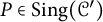 $P\in \mathrm {Sing}({\mathcal C'})$
corresponds to a pair of edges
 $\{y, \overline {y}\}$
for some
 $y\in \mathcal {Y}(\Gamma _{\mathcal C})$
. For each
 $v\in \mathcal {V}(\Gamma _{\mathcal C})$
, let
 $ D^{\prime }_v$
denote the irreducible component of
 ${\mathcal C'}$
corresponding to v. By contracting exceptional components of
 $\sigma $
, we can compute the degrees of irreducible components of
 $\mathcal C$
and the map
 $\boldsymbol {g}_{\mathcal C}\colon \mathcal {V}(\Gamma _{\mathcal C})\to \mathbb Z$
of genera from
 $ \mathrm {Cmb}(\mathcal C)$
. Hence, the combinatorics
 $ \mathrm {Cmb}(\mathcal C)$
can be regarded as the plumbing graph
 $$\begin{align*}\mathrm{Cmb}(\mathcal C)=(\Gamma_{\mathcal C}, \boldsymbol{g}_{\mathcal C},\boldsymbol{e}_{\mathcal C}; \mathrm{ Str}_{\mathcal C}) \end{align*}$$
together with the marking
 $ \mathrm {Str}_{\mathcal C}\subset \mathcal {V}(\Gamma _{\mathcal C})$
. Let
 $\mathscr {P}(\mathcal C)$
denote the plumbed manifold associated with
 $ \mathrm {Cmb}(\mathcal C)$
:
 $$\begin{align*}\mathscr{P}(\mathcal C):=\mathscr{P}(\Gamma_{\mathcal C},\boldsymbol{g}_{\mathcal C},\boldsymbol{e}_{\mathcal C}). \end{align*}$$
For two plane curves
 $\mathcal C_1, \mathcal C_2\subset {\mathbb {P}}^2$
, an equivalence map
 $\varphi \colon \mathrm { Cmb}(\mathcal C_1)\to \mathrm {Cmb}(\mathcal C_2)$
is an isomorphism
 $\varphi \colon \Gamma _{\mathcal C_1}\to \Gamma _{\mathcal C_2}$
of graphs such that
 $\varphi ( \mathrm {Str}_{\mathcal C_1})= \mathrm { Str}_{\mathcal C_2}$
,
 $\boldsymbol {g}_{\mathcal C_1}=\boldsymbol {g}_{\mathcal C_2}\circ \varphi ,$
and
 $\boldsymbol {e}_{\mathcal C_1}=\boldsymbol {e}_{\mathcal C_2}\circ \varphi $
. We say that
 $\mathcal C_1$
and
 $\mathcal C_2$
have the same combinatorics if there is an equivalence map
 $\varphi \colon \mathrm {Cmb}(\mathcal C_1)\to \mathrm {Cmb}(\mathcal C_2)$
.
3.2 The boundary manifold
$\mathscr {B}(\mathcal C)$

According to [Reference Durfee16], we define an algebraic neighborhood
 $\mathcal {T}(\mathcal C)$
of a plane curve
 $\mathcal C\subset {\mathbb {P}}^2$
as follows: Let
 $f\in \mathbb C[x_0,x_1,x_2]$
be a homogeneous polynomial of degree d defining
 $\mathcal C$
. Let
 $\eta _f\colon {\mathbb {P}}^2\to {\mathbb {R}}$
be the map defined by
 $$\begin{align*}\eta_f(x_0,x_1,x_2):= \frac{|f(x_0,x_1,x_2)|^2}{(|x_0|^2+|x_1|^2+|x_2|^2)^d}\in{\mathbb{R}} \end{align*}$$
for
 $(x_0:x_1:x_2)\in {\mathbb {P}}^2$
. Let
 $\mathcal {T}(\mathcal C):=\{(x_0:x_1:x_2)\in {\mathbb {P}}^2\mid \eta _f(x_0,x_1,x_2)\leq \delta \}$
for sufficiently small
 $\delta>0$
, which is called an algebraic neighborhood of
 $\mathcal C$
. By [Reference Łojasiewicz25],
 $\mathcal {T}(\mathcal C)$
is a regular neighborhood of
 $\mathcal C$
. By [Reference Durfee16],
 $\mathcal {T}(\mathcal C)$
is unique up to isotopy as an algebraic neighborhood. However, the author is not sure whether
 $\mathcal {T}(\mathcal C)$
is unique as a regular neighborhood. Let
 $\mathscr {B}(\mathcal C)$
be the boundary of
 $\mathcal {T}(\mathcal C)$
,
 $ \mathscr {B}(\mathcal C):=\partial \mathcal {T}(\mathcal C)$
, called the boundary manifold of
 $\mathcal C$
.
Remark 3.1 For any regular neighborhood
 $U(\mathcal C)$
of
 $\mathcal C$
, we may assume that
 $\mathcal {T}(\mathcal C)\subset U(\mathcal C)$
by taking sufficiently small
 $\delta>0$
.
Let
 $\sigma \colon Y\to {\mathbb {P}}^2$
be the minimal good embedded resolution of
 $\mathcal C$
, and put
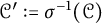 $\mathcal C':=\sigma ^{-1}(\mathcal C)$
. Since
 ${ \eta _f}\circ \sigma \colon Y\to {\mathbb {R}}$
is admissible in the sense of [Reference Mumford27], we can check that
 $\sigma ^{-1}(\mathcal {T}({\mathcal C}))$
is given by plumbing tubular neighborhoods
 $\mathcal {T}({ D'})$
of irreducible components
 ${ D'}$
of
 ${\mathcal C'}$
(cf. [Reference Hirzebruch, Neumann and Koh22, Section 8] and [Reference Mumford27, Section 1]). Note that, for each irreducible component
 ${ D'}\subset {\mathcal C'}$
, the Euler number of the
 $S^1$
-bundle
 $ \overline {p}_D\colon \partial \mathcal {T}(D')\to D'$
is equal to the self-intersection number of
 ${ D'}$
. From this point of view,
 $\mathscr {B}(\mathcal C)$
is constructed from
 $ \mathrm {Cmb}(\mathcal C)$
as follows. For
 $v\in \mathcal {V}(\Gamma _{\mathcal C})$
, put
 $$ \begin{align*} B_v&:=D^{\prime}_v\setminus U( \mathrm{Sing}(\mathcal C'))^\circ, & M_v&:=\overline{p}_{D_v}^{-1}(B_v), & p_v&:=\overline{p}_{D_v}|_{M_v}\colon M_v\longrightarrow B_v. \end{align*} $$
For
 $y\in \mathcal {Y}(\Gamma _{\mathcal C})$
, let
 $\partial B_{y}$
be the connected component of
 $\partial B_{t(y)}$
around the node
 $P_y$
of
 $\mathcal C'$
corresponding to y, and put
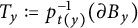 $T_y:=p_{t(y)}^{-1}(\partial B_{y})$
. We may assume that
 $\mathcal C'$
and
 $D^{\prime }_{t(y)}$
are locally defined at
 $P_y$
by
 $z_1z_2=0$
and
 $z_2=0$
, respectively, in
 $\mathbb {D}^2\times \mathbb {D}^2$
with coordinates
 $(z_1,z_2)$
, and that
 $T_y$
is a torus given by
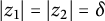 $|z_1|=|z_2|=\delta $
for small
 $\delta>0$
. Let
 $\tau _y\colon S^1\times S^1\to T_y$
be the trivialization given by
 $(z_1,z_2)\mapsto (\delta z_1,\delta z_2)$
. Then
 $\mathscr {B}(\mathcal C)$
is constructed by gluing
 $M_{t(y)}$
and
 $M_{t(\overline {y})}$
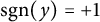
by (2.2) with
 $\mathrm {sgn}(y)=+1$
. Hence,
 $\mathscr {B}(\mathcal C)$
is a graph manifold with graph structure
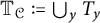 $\mathbb T_{\mathcal C}:=\bigcup _y T_y$
, where
 $T_{\overline {y}}$
is identified with
 $T_y$
in
 $\mathscr {B}(\mathcal C)$
for each
 $y\in \mathcal {Y}(\Gamma _{\mathcal C})$
. We call
 $\mathbb T_{\mathcal C}\subset \mathscr {B}(\mathcal C)$
the graph structure with respect to
 $ \mathrm { Cmb}(\mathcal C)$
. It follows from the definition of
 $\mathscr {P}(\mathcal C)$
that
 $\mathscr {B}(\mathcal C)$
is homeomorphic to
 $\mathscr {P}(\mathcal C)$
. Therefore, if two plane curves
 $\mathcal C_1,\mathcal C_2\subset {\mathbb {P}}^2$
have the same combinatorics, then there is a homeomorphism
 $h\colon \mathcal {T}(\mathcal C_1)\to \mathcal {T}(\mathcal C_2)$
with
 $h(\mathcal C_1)=\mathcal C_2$
.
3.3 Embedded topology in regular neighborhoods
Let
 $\mathcal C_1,\mathcal C_2\subset {\mathbb {P}}^2$
be two plane curves, and let
 $\sigma _i\colon Y_i\to {\mathbb {P}}^2$
be the minimal good embedded resolution of
 $\mathcal C_i$
. We put
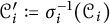 ${\mathcal C}^{\prime }_{i}:=\sigma _i^{-1}(\mathcal C_i)$
, and identify the combinatorics
 $ \mathrm {Cmb}(\mathcal C_i)$
with the corresponding plumbing graph, write
 $$\begin{align*}\mathrm{Cmb}(\mathcal C_i)=(\Gamma_i,\boldsymbol{g}_i,\boldsymbol{e}_i; \mathrm{Str}_i). \end{align*}$$
For
 $v_i\in \mathrm {Str}_i$
(resp.
 $v_i\in \mathcal {V}(\Gamma _i)$
), let
 $ D_{v_i}$
(resp.
 ${D}^{\prime }_{v_i}$
) be the irreducible component of
 $\mathcal C_i$
(resp.
 ${\mathcal C}^{\prime }_i$
) corresponding to
 $v_i$
. For
 $v_i\in \mathcal {V}(\Gamma _i)$
and
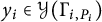
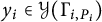
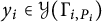
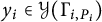
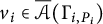
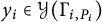
 $y_i\in \mathcal {Y}(\Gamma _i)$
, let
 $M_{v_i}$
,
 $B_{v_i}$
,
 $p_{v_i}$
,
 $T_{y_i}$
, and
 $\tau _{y_i}$
be as in Section 3.2. Let
 $ \mathbb T_i=\bigcup _{y_i} T_{y_i}\subset \mathscr {B}(\mathcal C_i)$
be the graph structure with respect to
 $ \mathrm { Cmb}(\mathcal C_i)$
.
Assume that there is a homeomorphism
 $h\colon U(\mathcal C_1)\to U(\mathcal C_2)$
with
 $h(\mathcal C_1)=\mathcal C_2$
for some regular neighborhoods
 $U(\mathcal C_i)$
of
 $\mathcal C_i$
. As in the proof of [Reference Artal Bartolo, Cogolludo-Agustín and Morales7, Theorem 2.2], h induces an isomorphism
 $$\begin{align*}\Psi_h^\infty\colon \pi_1(\mathscr{B}(\mathcal C_1))\longrightarrow\pi_1(\mathscr{B}(\mathcal C_2)). \end{align*}$$
The isomorphism
 $\Psi _h^\infty $
can be constructed as follows: Let
 $\mathcal {T}(\mathcal C_2)\subset h(U(\mathcal C_1))$
be an algebraic neighborhood of
 $\mathcal C_2$
, and let
 $\mathcal {T}(\mathcal C_1)\subset h^{-1}(\mathcal {T}(\mathcal C_2))$
be an algebraic neighborhood of
 $\mathcal C_1$
. Then there is an algebraic neighborhood
 $\mathcal {T}'(\mathcal C_2)\subset h(\mathcal {T}(\mathcal C_1))$
. Since
 $\mathscr {B}(\mathcal C_i)$
is homotopic to
 $\mathcal {T}(\mathcal C_i)\setminus \mathcal C_i$
, we obtain the homomorphism
 $$\begin{align*}\Psi_h^\infty\colon\pi_1(\mathscr{B}(\mathcal C_1))\cong\pi_1(\mathcal{T}(\mathcal C_1)\setminus\mathcal C_1)\overset{h_\ast}{\longrightarrow}\pi_1(\mathcal{T}(\mathcal C_2)\setminus\mathcal C_2)\cong\pi_1(\mathscr{B}(\mathcal C_2)). \end{align*}$$
Since we can similarly construct the inverse map of
 $\Psi _h^\infty $
, it is an isomorphism.
In [Reference Artal Bartolo, Cogolludo-Agustín and Morales7], it is also proved by using [Reference Waldhausen39, Corollary 6.5] that there exists a homeomorphism
 $\Psi _{\mathscr {B}}\colon \mathscr {B}(\mathcal C_1)\to \mathscr {B}(\mathcal C_2)$
with
 $\Psi _{\mathscr {B}\,\ast }=\Psi _h^\infty $
in several cases. Here, we construct such a homeomorphism
 $\Psi _{\mathscr {B}}\colon \mathscr {B}(\mathcal C_1)\to \mathscr {B}(\mathcal C_2)$
homotopic to
 $h|_{\mathscr {B}(\mathcal C_1)}$
in general case and prove that
 $\Psi _{\mathscr {B}}$
maps meridians of irreducible components of
 ${\mathcal C}^{\prime }_1$
to those of
 ${\mathcal C}^{\prime }_2$
.
Remark 3.2 We can construct a map
 $h'\colon \mathscr {B}(\mathcal C_1)\to \mathscr {B}(\mathcal C_2)$
homotopic to
 $h|_{\mathscr {B}(\mathcal C_1)}$
, which is homeomorphic outside of small regular neighborhoods of singular points, as follows.
By [Reference Brieskorn and Knörrer13, Theorem 21],
 $\mathcal C_1$
and
 $\mathcal C_2$
have the same singularity at each
 $P_1\in \mathcal C_1$
and
 $h(P_1)\in \mathcal C_2$
. By the isotopy theorem for closed tubular neighborhoods [Reference Hirsch21, Theorem 6.5], we may assume that h maps
 $\mathscr {B}(\mathcal C_1)\setminus U_{ \mathrm {Sing},1}$
to
 $\mathscr {B}(\mathcal C_2)\setminus U_{ \mathrm { Sing},2}$
homeomorphically for certain regular neighborhoods
 $U_{ \mathrm {Sing},i}:=U( \mathrm { Sing}(\mathcal C_i))$
. Let
 $\mathcal {T}_i(\mathcal C_2)$
(
 $i=1,2$
) be two algebraic neighborhoods of
 $\mathcal C_2$
such that
 $\mathcal {T}_1(\mathcal C_2)\subset h(\mathscr {B}(\mathcal C_1))\subset \mathcal {T}_2(\mathcal C_2)$
. By a certain deformation retract
 $\mathcal {T}_2(\mathcal C_2)\to \mathcal {T}_1(\mathcal C_2)$
, we obtain the desired map
 $h'\colon \mathscr {B}(\mathcal C_1)\to \mathscr {B}(\mathcal C_2)$
with
 $h'(\mathscr {B}(\mathcal C_1)\cap U_{ \mathrm { Sing},1})=\mathscr {B}(\mathcal C_2)\cap U_{ \mathrm {Sing},2}$
.
In particular, if
 $\mathcal C_1$
is smooth, then
 $\mathcal C_2$
is also smooth, and
 $h'$
is a homeomorphism. This implies
 $\deg \mathcal C_1=\deg \mathcal C_2$
, that is,
 $\mathcal C_1$
and
 $\mathcal C_2$
have the same combinatorics. Hence, we assume that
 $\mathcal C_i$
are singular below.
Assume that
 $\mathcal C_i$
are singular. We locally construct a homeomorphism of boundary manifolds around each singular point homotopic to h. Let
 $P_1$
be a singular point of
 $\mathcal C_1$
, and put
 $P_2:=h(P_1)$
. Let
 $U(P_i)\subset {\mathbb {P}}^2$
be a regular neighborhood of
 $P_i$
for each
 $i=1,2$
. We may assume that
 $$ \begin{align*} \mathscr{B}(\mathcal C_i,P_i):=\mathscr{B}(\mathcal C_i)\cap U(P_i) \subset \mathscr{B}(\mathcal C_i)\setminus\bigcup_{v_i\in \mathrm{Str}_i} { M_{v_i}^\circ} \end{align*} $$
is a connected component of the complement of the union of
 $\{{ M_{v_i}^\circ }\mid v_i\in \mathrm {Str}_i\}$
in
 $\mathscr {B}(\mathcal C_i)$
. We can regard
 $\mathscr {B}(\mathcal C_i,P_i)$
as a boundary framed graph manifold associated with the decorated plumbing graph
 $$\begin{align*}\Gamma_{\mathrm{dpg}}(\mathcal C_i,P_i)=(\Gamma_{i,P_i}, \boldsymbol{g}_{i,P_i}, \boldsymbol{e}_{i,P_i};\overline{\mathcal{A}}, \mathcal{A}) \end{align*}$$
defined as follows: If
 $P_i\in \mathcal C_i$
is not a node at which two distinct components intersect, then we define
 $\Gamma _{\mathrm {dpg}}(\mathcal C_i,P_i)$
by the following steps:
-
(I) let
$\overline {\mathcal {A}}(\Gamma _{i,P_i})$
be the subset of
$\mathcal {V}(\Gamma _i)$
consisting of vertices
$v_i$
with
$\sigma _i({ D^{\prime }_{v_i}})=\{P_i\}$
; -
(II)
$\mathcal {Y}(\Gamma _{i,P_i})$
is the subset of
$\mathcal {Y}(\Gamma _i)$
consisting of edges
$y_i$
with either
$t(y_i)\in \overline {\mathcal {A}}(\Gamma _{i,P_i})$
or
$o(y_i)\in \overline {\mathcal {A}}(\Gamma _{i,P_i})$
; -
(III)
$\mathcal {A}(\Gamma _{i,P_i})$
is in bijection with the set of edges
$y_i\in \mathcal {Y}(\Gamma _{i,P_i})$
with
$t(y_i)\notin \overline {\mathcal {A}}(\Gamma _{i,P_i})$
as edges of
$\Gamma _i$
; let
$v_{i,y_i}$
be the vertex of
$\mathcal {A}(\Gamma _{i,P_i})$
corresponding to
$y_i$
; -
(IV) for each
$y_i\in \mathcal {Y}(\Gamma _{i,P_i})$
, let
$t(y_i)$
be the same terminal vertex
$t(y_i)$
of
$y_i\in \mathcal {Y}(\Gamma _i)$
if
$t(y_i)\in \overline {\mathcal {A}}(\Gamma _{i,P_i})$
as a vertex of
$\Gamma _i$
; and put
$t(y_i):=v_{i,y_i}\in \mathcal {A}(\Gamma _{i,P_i})$
otherwise; -
(V) for each
$y_i\in \mathcal {Y}(\Gamma _{i,P_i})$
, put
$o(y_i):=t(\overline {y}_i)$
as edges of
$\Gamma _{i,P_i}$
; -
(VI)
$\boldsymbol {g}_{i,P_i}, \boldsymbol {e}_{i,P_i}\colon \overline {\mathcal {A}}(\Gamma _{i,P_i})\to \mathbb Z$
are the restrictions of
$\boldsymbol {g}_i$
and
$\boldsymbol {e}_i$
, respectively.








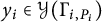













Note that
 $\Gamma _{\mathrm {dpg}}(\mathcal C_i,P_i)$
corresponds to the dual graph of the minimal good embedded resolution of the singularity
 $P_i\in \mathcal C_i$
locally. Hence,
 $\Gamma _{i,P_i}$
has no cycle.
According to [Reference Eisenbud and Neumann17, Chapter V], if
 $P_i\in \mathcal C_i$
is a node at which two distinct components intersect, we take the blowing-up at
 $P_i$
; replace
 $ \mathrm {Cmb}(\mathcal C_i)$
with the plumbing graph
 $\Gamma _{\mathrm {pg}}(\mathcal C_i)$
given by the blowing-up (
 $\mathrm {R1}^+$
) of
 $\mathop {\mathrm {Cmb}}(\mathcal C_i)$
at the edge corresponding to
 $P_i$
; and define
 $\Gamma _{\mathrm {dpg}}(\mathcal C_i,P_i)$
as above. Namely, if
 $P_i$
is a node of
 $\mathcal C_i$
, then
 $\Gamma _{\mathrm {dpg}}(\mathcal C_i,P_i)$
is the following decorated plumbing graph:

We denote the F-normal form of
 $\Gamma _{\mathrm {dpg}}(\mathcal C_i,P_i)$
by
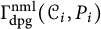
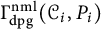
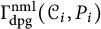
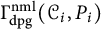
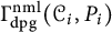 $\Gamma _{\mathrm {dpg}}^{\mathrm {nml}}(\mathcal C_i,P_i)$
. For
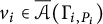 $v_i\in \overline {\mathcal {A}}(\Gamma _{i,P_i})$
and
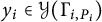 $y_i\in \mathcal {Y}(\Gamma _{i,P_i})$
, we may define
 $ p_{v_i}\colon M_{v_i}\to B_{v_i}$
,
 $ T_{y_i}$
and
 $ \tau _{y_i}\colon S^1\times S^1\to T_{y_i}$
as the same things for
 $\Gamma _{\mathrm {pg}}(\mathcal C_i)$
. Let
 $\mathbb T_{i.P_i}\subset \mathscr {B}(\mathcal C_i,P_i)$
be the graph structure with respect to
 $\Gamma _{\mathrm {dpg}}(\mathcal C_i,P_i)$
.
Note that
 $\mathcal {A}(\Gamma _{i,P_i})$
corresponds to the set of local branches of
 $\mathcal C_i$
at
 $P_i$
. Hence, h induces a bijection
 $$\begin{align*}\xi_{h,P_1}\colon\mathcal{A}(\Gamma_{1,P_1})\longrightarrow\mathcal{A}(\Gamma_{2,P_2}) \end{align*}$$
since
 $h(\mathcal C_1)=\mathcal C_2$
. Let
 $h_{P_1}\colon \mathscr {B}(\mathcal C_1,P_1)\to \mathscr {B}(\mathcal C_2,P_2)$
be the restriction of
 $h'\colon \mathscr {B}(\mathcal C_1)\to \mathscr {B}(\mathcal C_2)$
constructed in Remark 3.2. We have the induced isomorphism
 $$\begin{align*}h_{P_1\ast}\colon \pi_1(\mathscr{B}(\mathcal C_1,P_1))\longrightarrow\pi_1(\mathscr{B}(\mathcal C_2,P_2)) \end{align*}$$
of fundamental groups
 $\pi _1(\mathscr {B}(\mathcal C_i,P_i))$
such that
 $h_{P_1\ast }(i_{y_1\ast }(\pi _1({ T_{y_1}})))=i_{y_2\ast }(\pi _1({ T_{y_2}}))$
for each
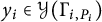 $y_i\in \mathcal {Y}(\Gamma _{i,P_i})$
with
 $t(y_1)\in \mathcal {A}(\Gamma _{1,P_1})$
and
 $t(y_2)=\xi _{h,P_1}(t(y_1))$
, where
 $i_{y_i}\colon { T_{y_i}}\to \mathscr {B}(\mathcal C_i,P_i)$
is the inclusion map. Note that it follows from [Reference Brieskorn and Knörrer13, III, Theorem 21] that there exists an isomorphism
 $$ \begin{align} \varphi_{P_1}\colon\Gamma_{\mathrm{dpg}}(\mathcal C_1,P_1)\longrightarrow \Gamma_{\mathrm{dpg}}(\mathcal C_2,P_2) \end{align} $$
satisfying
 $\varphi _{P_1}|_{\mathcal {A}(\Gamma _{1,P_1})}=\xi _{h,P_1}$
, and hence
 $\mathscr {B}(\mathcal C_i,P_i)$
are homeomorphic.
Remark 3.3 We can prove from
 $\varphi _{P_1}$
for each
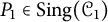 $P_1\in \mathrm {Sing}(\mathcal C_1)$
that
 $\mathcal C_1$
and
 $\mathcal C_2$
have the same combinatorics if they have the same embedded topology in regular neighborhoods. Indeed, if
 $v_i\in \mathrm {Str}_i$
satisfy
 $ h(D_{v_1})=D_{v_2}$
, then we have
 $\boldsymbol {g}_1(v_1)=\boldsymbol {g}_2(v_2)$
, and
 $$\begin{align*}\boldsymbol{g}_i(v_i)=\frac{(d_i-1)(d_i-2)}{2}-{ \sum_{P_i\in \mathrm{Sing}(D_{v_i})}\delta_{D_{v_i},P_i}}, \end{align*}$$
where
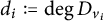 $d_i:=\deg { D_{v_i}}$
, and
 $\delta _{ D_{v_i},P_i}\in \mathbb Z$
is the delta invariant of
 $ D_{v_i}$
at
 $P_i\in \mathrm { Sing}({ D_{v_i}})$
. The existence of
 $\varphi _{P_1}$
implies
 $\sum \delta _{ D_{v_1},P_1}=\sum \delta _{ D_{v_2},P_2}$
. If
 $d_1\leq 2$
, then we obtain
 $d_1=d_2$
by Remark 3.2. If
 $d_1>2$
, then
 $d_1=d_2$
follows from
 $d_i>0$
. Hence, we have
 $\boldsymbol {e}_1(v_1)=\boldsymbol {e}_2(v_2)$
by
 $d_1=d_2$
and the existence of
 $\varphi _{P_1}$
. Therefore, we can construct an equivalence map
 $\varphi \colon \mathrm {Cmb}(\mathcal C_1)\to \mathrm { Cmb}(\mathcal C_2)$
. The arguments in Section 3.2 and this remark prove Fact 1.1.
We here construct a homeomorphism
 $\mathfrak {g}_{P_1}\colon \mathscr {B}(\mathcal C_1,P_1)\to \mathscr {B}(\mathcal C_2,P_2),$
which is homotopic to
 $h_{P_1}$
and satisfies certain properties. Put
 $E:=(\begin {smallmatrix} 1&0\\0&1 \end {smallmatrix})$
, the identity matrix.
Lemma 3.4 Assume that
 $P_1$
is a node of
 $\mathcal C_1$
. Then
 $P_2$
is a node of
 $\mathcal C_2$
, and there exists a homeomorphism
 $\mathfrak {g}_{P_1}\colon \mathscr {B}(\mathcal C_1,P_1)\to \mathscr {B}(\mathcal C_2,P_2)$
such that
-
(i)
$\mathfrak {g}_{P_1}$
is homotopic to
$h_{P_1}$
; -
(ii)
$\mathfrak {g}_{P_1}{ (T_{y_1})=T_{y_2}}$
for
$y_i\in \mathcal {Y}(\Gamma _{i,P_i})$
with
$t(y_i)\in \mathcal {A}(\Gamma _{i,P_i})$
and
$t(y_2)=\xi _{h,P_1}(t(y_1))$
; -
(iii)
$\mathfrak {g}_{P_1}$
preserves trivializations of the boundaries, that is, for
$y_i\in \mathcal {Y}(\Gamma _{i,P_i})$
with
$t(y_i)\in \mathcal {A}(\Gamma _{i,P_i})$
and
$t(y_2)=\xi _{h,P_1}(t(y_1))$
,
${ \tau _{y_2}^{-1}}\circ \mathfrak {g}_{P_1}\circ { \tau _{y_1}}\colon S^1\times S^1\to S^1\times S^1$
is given by a matrix
$\alpha E$
for some
$\alpha =\pm 1$
; -
(iv) for
$v_i\in \overline {\mathcal {A}}(\Gamma _{i,P_i})$
,
$\mathfrak {g}_{P_1}$
preserves fibers of
$v_1$
and
$v_2$
, that is, for any fiber
$F_1$
of
$ p_{v_1}$
,
$\mathfrak {g}_{P_1}(F_1)$
is a fiber of
$ p_{v_2}$
.













Moreover,
 $\alpha =1$
if and only if h maps a meridian of
 $ D_{t(y_1)}$
to a meridian of
 $ D_{t(y_2)}$
for some
 $y_i\in \mathcal {Y}(\Gamma _{i,P_i})$
with
 $t(y_2)=\xi _{h,P_1}(t(y_1))$
, where arrowheads in
 $\mathcal {A}(\Gamma _{i,P_i})$
are regarded as vertices in
 $ \mathrm {Str}_{i}$
.
Proof By [Reference Brieskorn and Knörrer13, III, Theorem 21],
 $P_2$
is also a node of
 $\mathcal C_2$
. We may identify
 $\mathscr {B}(\mathcal C_i,P_i)$
with
 $I\times S^1\times S^1$
so that
 $h_{P_1}(\{j\}\times S^1\times S^1)=\{j\}\times S^1\times S^1$
for each
 $j\in \partial I$
. Let
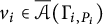 $v_i\in \overline {\mathcal {A}}(\Gamma _{i,P_i})$
be the unique vertex for each
 $i=1,2$
. For
 $i=1,2$
and
 $j\in \partial I$
, let
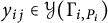 $y_{ij}\in \mathcal {Y}(\Gamma _{i,P_i})$
be the edge satisfying
 $w_{ij}:=t(y_{ij})\in \mathcal {A}(\Gamma _{i,P_i})$
and
 ${ T_{y_{ij}}}=\{j\}\times S^1\times S^1$
. The trivialization
 $\tau _{ij}:={ \tau _{y_{ij}}}$
is determined by a meridian
 $\mathfrak {m}_{ij}$
of
 $ D_{w_{ij}}$
and a fiber
 $\mathfrak {f}_{i}$
of
 $ p_{v_i}\colon M_{v_i}\to B_{v_i}$
. It follows from
 $\boldsymbol {e}_{i,P_i}(v_i)=-1$
that
 $\mathfrak {f}_i=\mathfrak {m}_{i0}\mathfrak {m}_{i1}$
in
 $\pi _1(\mathscr {B}(\mathcal C_i,P_i))$
. By [Reference Artal Bartolo, Bannai, Shirane and Tokunaga3, Proposition 3.4 and Remark 3.5], there is
 $\alpha \in \{\pm 1\}$
such that
 $h_{P_1\ast }(\mathfrak {m}_{1j})=\mathfrak {m}_{2j}^\alpha $
for each
 $j\in \partial I$
. Since
 $\boldsymbol {e}_1(v_1)=\boldsymbol {e}_2(v_2)=-1$
, there is a homeomorphism
 $\mathfrak {g}_{P_1}\colon \mathscr {B}(\mathcal C_1,P_1)\to \mathscr {B}(\mathcal C_2,P_2)$
preserving fibers and
 $\mathfrak {g}_{P_1\ast }(\mathfrak {m}_{1j})=\mathfrak {m}_{2j}^\alpha $
for
 $j\in \partial I$
. Since
 $h_{P_1\ast }=\mathfrak {g}_{P_1\ast }$
, and the universal covering of a torus is not compact,
 $h_{P_1}$
is homotopic to
 $\mathfrak {g}_{P_1}$
by [Reference Olum30, Theorem I].
Note that the homeomorphism
 $\mathfrak {g}_{P_1}$
in Lemma 3.4 is orientation-preserving by condition (iii). We consider the case where
 $P_1$
is not a node of
 $\mathcal C_1$
.
Lemma 3.5 (cf. [Reference Neumann28, Theorem 8.2])
If
 $P_i\in \mathcal C_i$
is a singular point which is not node, then the F-normal form
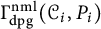 $\Gamma _{\mathrm {dpg}}^{\mathrm {nml}}(\mathcal C_i,P_i)$
is obtained from
 $\Gamma _{\mathrm {dpg}}(\mathcal C_i,P_i)$
by applying the following operations to
 $\Gamma _{\mathrm {dpg}}(\mathcal C_i,P_i)$
wherever possible:

Furthermore,
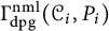 $\Gamma _{\mathrm {dpg}}^{\mathrm {nml}}(\mathcal C_i,P_i)$
satisfies the following:
-
(i) All edges of
$\Gamma _{\mathrm {dpg}}^{\mathrm {nml}}(\mathcal C_i,P_i)$
are
$(+)$
-edges. -
(ii) Any vertex
$v_i$
of
$\Gamma _{\mathrm {dpg}}^{\mathrm {nml}}(\mathcal C_i,P_i)$
satisfies
$\boldsymbol {g}(v_i)\geq -1$
. -
(iii) Any vertex
$v_i$
of
$\Gamma _{\mathrm {dpg}}^{\mathrm {nml}}(\mathcal C_i,P_i)$
with
$\boldsymbol {g}(v_i)=-1$
satisfies
$\boldsymbol {d}(v_i)=1$
,
$\boldsymbol {e}(v_i)\geq 0$
, and if
$\boldsymbol {e}(v_i)=0$
, the maximal chain adjoining
$v_i$
has length
$\geq 1$
. -
(iv)
$\Gamma _{\mathrm {dpg}}(\mathcal C_i,P_i)$
is uniquely determined by
$\Gamma _{\mathrm {dpg}}^{\mathrm {nml}}(\mathcal C_i,P_i)$
.






Proof Since the intersection form of
 $\Gamma _{\mathrm {dpg}}(\mathcal C_i,P_i)$
is negative definite (cf. [Reference Mumford27]), we can apply the argument of [Reference Neumann28, Section 8]. By [Reference Neumann28, Theorem 8.2],
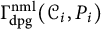 $\Gamma _{\mathrm {dpg}}^{\mathrm {nml}}(\mathcal C_i,P_i)$
is obtained by the operations in the statement since
 $\Gamma _{\mathrm {dpg}}(\mathcal C_i,P_i)$
has boundary vertices. It is clear that (i) holds. Since any vertex of
 $\Gamma _{\mathrm {dpg}}(\mathcal C_i,P_i)$
has nonnegative genus, any vertex
 $v_i$
of
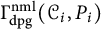 $\Gamma _{\mathrm {dpg}}^{\mathrm {nml}}(\mathcal C_i,P_i)$
with
 $\boldsymbol {g}(v_i)\leq -1$
is given by the operations in the statement. Therefore, we obtain (ii)–(iv).
Remark 3.6 The first operation in Lemma 3.5 can be done by
 $-e-1$
times blowing-ups (
 $\mathrm {R1}^-$
), an
 ${\mathbb {R}}{\mathbb {P}}^2$
-absorption (R2), a blowing-up (
 $\mathrm {R1}^+$
), and
 $-e-2$
times blowing-downs (
 $\mathrm {R1}^+$
) (see Remark 2.5). The second operation in Lemma 3.5 can be done by a blowing-up (
 $\mathrm {R1}^-$
),
 $b-1$
times blowing-downs (
 ${\mathrm {R1}}^+$
), and an
 ${\mathbb {R}}{\mathbb {P}}^2$
-absorption (R2).
Lemma 3.7 Assume that
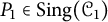 $P_1\in \mathrm {Sing}(\mathcal C_1)$
is not a node. Then there exists a homeomorphism
 $\mathfrak {g}_{P_1}'\colon \mathscr {B}(\mathcal C_1,P_1)\to \mathscr {B}(\mathcal C_2,P_2)$
homotopic to
 $h_{P_1}$
.
Proof Let
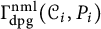 $\Gamma _{\mathrm {dpg}}^{\mathrm {nml}}(\mathcal C_i,P_i)$
be the F-normal form of
 $\Gamma _{\mathrm {dpg}}(\mathcal C_i,P_i)$
. By Lemma 3.5,
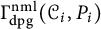 $\Gamma _{\mathrm {dpg}}^{\mathrm {nml}}(\mathcal C_i,P_i)$
is connected. For each
 $i=1,2$
, let
 $\mathcal {S}_i$
be a subset of edges of
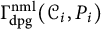 $\Gamma _{\mathrm {dpg}}^{\mathrm {nml}}(\mathcal C_i,P_i)$
such that
 $\mathcal {S}_i$
contains precisely one edge of each maximal chain of
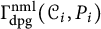 $\Gamma _{\mathrm {dpg}}^{\mathrm {nml}}(\mathcal C_i,P_i)$
which is not incident to a boundary vertex (see [Reference Neumann28, Section 4] or Appendix B.1). By Theorem B.1,
 $ \mathbb T_{\mathcal {S}_i}:=\bigcup _{y_i\in \mathcal {S}_i}T_{y_i}$
is the reduced graph structure of
 $\mathscr {B}(\mathcal C_i,P_i)$
. Hence,
 $\mathscr {B}(\mathcal C_i,P_i)$
can be regarded as a reduced graph manifold. Then
 $\mathscr {B}(\mathcal C_i,P_i)$
is irreducible by [Reference Waldhausen38, Theomre 7.1]. Since
 $\mathscr {B}(\mathcal C_i,P_i)$
is not a solid torus,
 $\mathscr {B}(\mathcal C_i,P_i)$
is boundary-irreducible and sufficiently large by [Reference Waldhausen38, Lemma 7.2]. Hence, it follows from [Reference Waldhausen39, Theorem 6.1] that there is a homeomorphism
 $\mathfrak {g}_{P_1}'\colon \mathscr {B}(\mathcal C_1,P_1)\to \mathscr {B}(\mathcal C_2,P_2)$
such that
 $\mathfrak {g}^{\prime }_{P_1}$
is homotopic to
 $h_{P_1}$
.
We prove that the homeomorphism
 $\mathfrak {g}^{\prime }_{P_1}$
is orientation-preserving.
Lemma 3.8 Assume that
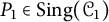 $P_1\in \mathrm {Sing}(\mathcal C_1)$
is not a node of
 $\mathcal C_1$
, and let
 $\mathfrak {g}_{P_1}'$
be the homeomorphism in Lemma 3.7. Then
 $\mathfrak {g}^{\prime }_{P_1}$
is orientation-preserving.
Proof Assume that
 $\mathfrak {g}_{P_1}'$
is orientation-reversing. Let
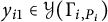 $y_{i1}\in \mathcal {Y}(\Gamma _{i,P_i})$
be edges with
 $t({ y_{i1}})\in \mathcal {A}(\Gamma _{i,P_i})$
and
 $\xi _{h,P_1}(t({ y_{11}}))={ y_{21}}$
. Since the isomorphism
 $\varphi _{P_1}$
satisfies
 $\varphi _{P_1}|_{\mathcal {A}(\mathcal C_{1,P_1})}=\xi _{h,P_1}$
, the maximal chains incident to
 $ y_{i1}$
are the same form:

where
 $-b_j\leq -2$
are the Euler numbers of corresponding vertices, and
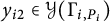 $y_{i2}\in \mathcal {Y}(\Gamma _{i,P_i})$
are edges such that
 $v_{i2}=t(y_{i2})$
and
 $\boldsymbol {d}(v_{i2})\geq 3$
for
 $i=1,2$
. Let
 $v_{i1}\in \mathrm {Str}_i$
be the vertices corresponding to
 $t(y_{i1})\in \mathcal {A}(\Gamma _{i,P_i})$
. Let
 $T_{ij}$
be the boundary component
 $ T_{y_{ij}}$
of
 $M_{v_{ij}}$
corresponding
 $y_{ij}$
for each
 $i,j=1,2$
. By [Reference Neumann28, Lemma 5.3],
 $T_{i1}$
and
 $T_{i2}$
are identified in
 $\mathscr {B}(\mathcal C_i)$
via homeomorphism given by the matrix
 $$\begin{align*}B_k:=\begin{pmatrix} d_k & c_k \\ - d_{k-1} & -c_{k-1} \end{pmatrix}, \end{align*}$$
where
 $c_i, d_i\in \mathbb Z$
are coprime integers such that
 $c_i/d_i$
is equal to the continued fraction
 $[b_1,\dots ,b_i]$
for each
 $i=1,\dots ,k$
(see [Reference Neumann28, Lemma 5.2] for details). Note that
 $c_{-1}=0$
,
 $c_0=1$
,
 $d_{-1}=-1$
,
 $d_0=0$
, and
 $\det B_k=-1$
. By [Reference Artal Bartolo, Bannai, Shirane and Tokunaga3, Proposition 3.4] and [Reference Waldhausen38, Theorem 5.5], we may assume that
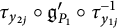 $ \tau _{y_{2j}}\circ \mathfrak {g}^{\prime }_{P_1}\circ \tau _{y_{1j}}^{-1}$
is the homeomorphism of
 $S^1\times S^1$
given by the matrix
 $$\begin{align*}H_j:=\begin{pmatrix} \alpha_j&0\\ \beta_j & -\alpha_j \end{pmatrix} \end{align*}$$
for each
 $j=1,2$
, where
 $\alpha _j\in \{\pm 1\}$
and
 $\beta _j\in \mathbb Z$
. Hence, we have the following commutative diagram:

The
 $(1,2)$
entry of
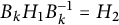 $B_kH_1B_k^{-1}=H_2$
is
 $(2\alpha _1 d_k+\beta _1 c_k)c_k=0$
. Since
 $\gcd (c_k,d_k)=1$
,
 $c_k\geq k+1,$
and
 $d_k\geq k$
by [Reference Neumann28, Lemma 5.2(ii)], we obtain either
 $d_k=0$
or
 $c_k=2$
. If
 $d_k=0$
, then
 $k=0$
,
 $\beta _1=0$
, and
 $H_2=-H_1$
. If
 $c_k=2$
, then we have
 $k=1$
,
 $d_k=1$
,
 $b_1=2$
,
 $\beta _1=-\alpha _1,$
and
 $H_2=-H_1$
. Thus, we can construct
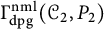 $\Gamma _{\mathrm {dpg}}^{\mathrm {nml}}(\mathcal C_2,P_2)$
from
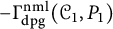 $-\Gamma _{\mathrm {dpg}}^{\mathrm {nml}}(\mathcal C_1,P_1)$
by Theorem B.2.
By the above fact, we can apply the argument of [Reference Neumann28, Section 9] as follows. By Theorem B.2(ii) and Lemma 3.5(iii),
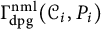 $\Gamma _{\mathrm {dpg}}^{\mathrm {nml}}(\mathcal C_i,P_i)$
for
 $i=1,2$
have no vertex v with
 $\boldsymbol {g}(v)=-1$
. Hence,
 $\Gamma _{\mathrm {dpg}}(\mathcal C_i,P_i)=\Gamma _{\mathrm {dpg}}^{\mathrm {nml}}(\mathcal C_i,P_i)$
for
 $i=1,2$
by Lemma 3.5, and
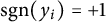 $\mathrm {sgn}(y_i)=+1$
for any
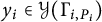 $y_i\in \mathcal {Y}(\Gamma _{i,P_i})$
. Since
 $\Gamma _{i,P_i}$
is the dual graph of embedded resolution of the singularity
 $P_i\in \mathcal C_i$
,
 $\Gamma _{i,P_i}$
has no cycle for each
 $i=1,2$
. Moreover, there is
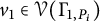 $v_1\in \mathcal {V}(\Gamma _{1,P_i})$
with
 $\boldsymbol {d}(v_1)\geq 3$
since
 $P_1$
is not node. Let
 $$\begin{align*}\Gamma_{\mathrm{dpg}}^{1,v_1}=(\Gamma_{1,P_1}^{v_1},\boldsymbol{g}_{1,P_1}^{v_1},\boldsymbol{e}_{1,P_1}^{v_1};\overline{\mathcal{A}},\mathcal{A})\end{align*}$$
be the full subgraph of
 $\Gamma _{\mathrm {dpg}}(\mathcal C_1,P_1)$
such that
 $\mathcal {V}(\Gamma _{1,P_1}^{v_1})$
consists of
 $v_1$
, all vertices on maximal chains adjoining
 $v_1$
and all boundary vertices adjacent to
 $v_1$
. The decorated plumbing graph
 $\Gamma _{\mathrm {dpg}}^{1,v_1}$
is a star-shaped decorated plumbing graph, and
 $\mathscr {P}(\Gamma _{\mathrm {dpg}}^{1,v_1})$
is a Seifelt manifold. Let
 $\widetilde {\Gamma }_{\mathrm {dpg}}^{1,v_1}$
be the F-normal form of
 $-\Gamma _{\mathrm {dpg}}^{1,v_1}$
. By Theorem B.2,
 $\widetilde {\Gamma }_{\mathrm {dpg}}^{1,v_1}$
is also a star-shaped decorated plumbing graph and is a subgraph of
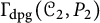 $\Gamma _{\mathrm {dpg}}(\mathcal C_2,P_2)$
. Since the intersection form
 $S(\Gamma _{\mathrm {dpg}}^{1,v_1})$
is negative definite, the Euler number of the Seifelt manifold
 $\mathscr {P}(\Gamma _{\mathrm {dpg}}^{1,v_1})$
is negative by Theorem B.4. Thus, the Euler number of
 $\mathscr {P}(\widetilde {\Gamma }_{\mathrm {dpg}}^{1,v_1})=\mathscr {P}(-\Gamma _{\mathrm {dpg}}^{1,v_1})$
is positive by the equality (B.2), which is contradiction to Theorem B.3 since
 $\widetilde {\Gamma }_{\mathrm {dpg}}^{1,v_1}$
is a subgraph of
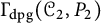 $\Gamma _{\mathrm {dpg}}(\mathcal C_2,P_2)$
, and the intersection form
 $S(\widetilde {\Gamma }_{\mathrm {dpg}}^{1,v_1})$
is negative definite. Therefore,
 $\mathfrak {g}^{\prime }_{P_1}$
is orientation-preserving.
Lemma 3.9 Assume that
 $P_1\in \mathrm {Sing}\mathcal C_1$
is not a node of
 $\mathcal C_1$
. There exists a homeomorphism
 $\mathfrak {g}_{P_1}\colon \mathscr {B}(\mathcal C_1,P_1)\to \mathscr {B}(\mathcal C_2,P_2)$
such that
-
(i)
$\mathfrak {g}_{P_1}$
is homotopic to
$h_{P_1}$
; -
(ii)
$\mathfrak {g}_{P_1}(\mathbb T_{1,P_1})=\mathbb T_{2,P_2}$
; -
(iii)
$\mathfrak {g}_{P_1}({ M_{v_1}})={ M_{\varphi _{P_1}(v_1)}}$
for each
$v_1\in \overline {\mathcal {A}}(\Gamma _{1})$
, where
$\varphi _{P_1}\colon \Gamma _{\mathrm {dpg}}(\mathcal C_1,P_1)\to \Gamma _{\mathrm {dpg}}(\mathcal C_2,P_2)$
is the isomorphism in (3.1); -
(iv) there is
$\alpha \in \{\pm 1\}$
such that
${ \tau _{y_2}\circ \mathfrak {g}_{P_1}\circ \tau _{y_1}}\colon S^1\times S^1\to S^1\times S^1$
is given by
$\alpha E$
for any
$y_1\in \mathcal {Y}(\Gamma _{1,P_1})$
with
$t(y_1)\in \mathcal {A}(\Gamma _{1,P_1})$
and
$y_2:=\varphi _{P_1}(y_1)$
; -
(v) for each
$v_1\in \overline {\mathcal {A}}(\Gamma _{1,P_1})$
,
$\mathfrak {g}_{P_1}$
preserves fibers of
$v_1$
and
$v_2=\varphi _{P_1}(v_1)\in \overline {\mathcal {A}}(\Gamma _{2,P_2})$
.









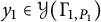

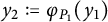
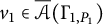



Moreover,
 $\alpha =1$
if and only if h maps a meridian of
 $ D_{t(y_1)}$
to a meridian of
 $ D_{t(y_2)}$
for some
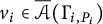 $v_i\in \overline {\mathcal {A}}(\Gamma _{i,P_i})$
with
 $t(y_i)\in \mathcal {A}(\Gamma _{i,P_i})$
and
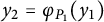 $y_2=\varphi _{P_1}(y_1)$
.
Proof We construct the desired homeomorphism
 $\mathfrak {g}_{P_1}$
by deforming
 $\mathfrak {g}^{\prime }_{P_1}$
in Lemma 3.7. Let
 $\mathcal {S}_i$
be the subset of edges of
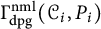 $\Gamma _{\mathrm {dpg}}^{\mathrm {nml}}(\mathcal C_i,P_i)$
as in the proof of Lemma 3.7, and put
 $ \mathbb T_{\mathcal {S}_i}:=\bigcup _{y_i\in \mathcal {S}_i}T_{y_i}$
which is a reduce graph structure of
 $\mathscr {B}(\mathcal C_i,P_i)$
. By [Reference Waldhausen38, Theorem 8.1] and Lemma 3.8, there is an isotopy
 $\mathfrak {h}_{u}\colon \mathscr {B}(\mathcal C_1,P_1)\to \mathscr {B}(\mathcal C_2,P_2)$
(
 ${0\leq u\leq 1}$
), which is constant on
 $\partial \mathscr {B}(\mathcal C_i,P_i)$
and satisfies
 $\mathfrak {h}_{0}=\mathfrak {g}^{\prime }_{P_1}$
and
 $ \mathfrak {h}_1(\mathbb T_{\mathcal {S}_1})=\mathbb T_{\mathcal {S}_2}$
.
Let
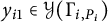 $y_{i1}\in \mathcal {Y}(\Gamma _{i,P_i})$
be edges satisfying
 $t(y_{i1})\in \mathcal {A}(\Gamma _{i,P_i})$
and
 $\varphi _{P_1}(y_{11})=y_{21}$
. For each
 $i=1,2$
, let
 $\mathfrak {c}_i$
be the maximal chain incident to
 $t(y_{i1})$
, and let
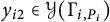 $y_{i2}\in \mathcal {Y}(\Gamma _{i,P_i})$
be the edge on
 $\mathfrak {c}_i$
such that
 $\boldsymbol {d}(t(y_{i2}))>2$
as in (3.2). By the same argument in the proof of Lemma 3.8, we may assume that
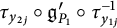 $ \tau _{y_{2j}}\circ \mathfrak {g}^{\prime }_{P_1}\circ \tau _{y_{1j}}^{-1}$
is given by
 $$\begin{align*}H_j:=\begin{pmatrix} \alpha_j&0\\ \beta_j & \alpha_j \end{pmatrix} \end{align*}$$
for each
 $j=1,2$
, where
 $\alpha _j\in \{\pm 1\}$
and
 $\beta _j\in \mathbb Z$
. It follows from the diagram (3.3) that
 $\alpha _1=\alpha _2$
and
 $\beta _j=0$
for
 $j=1,2$
.
For
 $y_i\in \mathcal {S}_i$
(
 $i=1,2$
) with
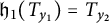 $ \mathfrak {h}_{1}(T_{y_1})=T_{y_2}$
, the maximal chains of
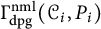 $\Gamma _{\mathrm {dpg}}^{\mathrm {nml}}(\mathcal C_i,P_i)$
containing
 $y_i$
have the same number of edges. Since each maximal chain of
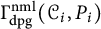 $\Gamma _{\mathrm {dpg}}^{\mathrm {nml}}(\mathcal C_i,P_i)$
corresponds to a part homeomorphic to
 $I\times S^1\times S^1$
in
 $\mathscr {B}(\mathcal C_i,P_i)$
, there is an isotopy
 $\mathfrak {h}_{u}\colon \mathscr {B}(\mathcal C_1,P_1)\to \mathscr {B}(\mathcal C_2,P_2)$
(
 $1\leq u\leq 2$
), which is constant on
 $\partial \mathscr {B}(\mathcal C_i,P_i)$
and satisfies
 $\mathfrak {h}_{2}(\mathbb T_{1,P_1}^{\mathrm {nml}})=\mathbb T_{2,P_2}^{\mathrm {nml}}$
, where
 $\mathbb T_{i,P_i}^{\mathrm {nml}}$
is the graph structure corresponding to
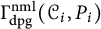 $\Gamma _{\mathrm {dpg}}^{\mathrm {nml}}(\mathcal C_i,P_i)$
. Tori in
 $\mathbb T_{i,P_i}$
exchanged by the operations in Lemma 3.5 are in the
 $S^1$
-bundle over the Möbius band studied in [Reference Waldhausen38, Section 3], and the tori give reduced graph structure of the
 $S^1$
-bundle. Hence, there is an isotopy
 $\mathfrak {h}_{u}\colon \mathscr {B}(\mathcal C_1,P_1)\to \mathscr {B}(\mathcal C_2,P_2)$
(
 $2\leq u\leq 3$
) by Theorem 2.2, which is constant on
 $\partial \mathscr {B}(\mathcal C_i,P_i)$
and satisfies
 $\mathfrak {h}_{3}(\mathbb T_{1,P_1})=\mathbb T_{2,P_2}$
.
If
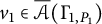 $v_{1}\in \overline {\mathcal {A}}(\Gamma _{1,P_1})$
is not on any chain of
 $\Gamma _{\mathrm {dpg}}(\mathcal C_1,P_1)$
, and
 $v_2:=\varphi _{P_1}(v_1)\in \overline {\mathcal {A}}(\Gamma _{2,P_2})$
, then, for a fiber
 $ F_{v_1}$
of
 $v_1$
, the image
 $ \mathfrak {h}_{3}(F_{v_1})$
is ambient isotopic in
 $ M_{v_2}$
to a fiber
 $ F_{v_2}$
of
 $v_2$
by Theorem A.6. If
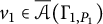 $v_1\in \overline {\mathcal {A}}(\Gamma _{1,P_1})$
is on a chain of
 $\Gamma _{\mathrm {dpg}}(\mathcal C_1,P_1)$
, then the argument of [Reference Neumann28, pp. 322–323] shows that, for a fiber
 $ F_{v_1}$
of
 $v_1$
, the image
 $ \mathfrak {h}_{3}(F_{v_1})$
is homotopic in
 $ M_{v_2}$
to a fiber
 $ F_{v_2}$
of
 $v_2$
(cf. [Reference Laufer24, Chapter II]).
For
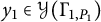 $y_1\in \mathcal {Y}(\Gamma _{1,P_1})$
with
 $t(y_1), t(\overline {y}_1)\notin \mathcal {A}(\Gamma _{1,P_1})$
, we can identify
 $ T_{\overline {y}_1}$
with
 $ T_{y_1}$
in
 $\mathscr {B}(\mathcal C_1,P_1)^\circ $
. Let
 $y_{i,1},\dots ,y_{i,r}\in \mathcal {Y}(\Gamma _{i,P_i})$
be edges such that
 $$ \begin{align*} & t(y_{i,j})\in\overline{\mathcal{A}}(\Gamma_{i,P_i}), && y_{i,j'}\notin\{y_{i,j},\overline{y}_{i,j}\} \quad \text{if } j\ne j', \\ & \varphi_P(y_{1,j})=y_{2,j}, && \mathcal{Y}(\Gamma_{i,P_i})=\{y_{i,j}, \overline{y}_{i,j}\mid j=1,\dots,r\}. \end{align*} $$
By Lemma A.4, there is an isotopy
 $\mathfrak {h}_{u}$
(
 $3\leq u\leq 4$
) from
 $\mathfrak {h}_{3}$
, which is constant on
 $\partial \mathscr {B}(\mathcal C_i,P_i)$
and preserves graph structures
 $\mathbb T_{i,P_i}$
, such that
 $\mathfrak {h}_{4}$
maps every fiber of
 $t(\overline {y}_{1,j})$
in
 $ T_{\overline {y}_{1,j}}$
to a fiber of
 $t(\overline {y}_{2,j})$
in
 $ T_{\overline {y}_{2,j}}$
. Since each fiber
 $F_{i,j}\subset { T_{y_{i,j}}}$
of
 $t(y_{i,j})$
intersects at just one point with each fiber
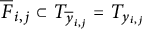 $ \overline {F}_{i,j}\subset T_{\overline {y}_{i,j}}=T_{y_{i,j}}$
of
 $t(\overline {y}_{i,j})$
, there is an isotopy
 $\mathfrak {h}_{u}$
(
 $4\leq u\leq 5$
) from
 $\mathfrak {h}_{4}$
such that
 $$ \begin{align*} & \mathfrak{h}_{u}(\mathbb T_{1,P_1})=\mathbb T_{2,P_2}, && \mathfrak{h}_{u}(\overline{F}_{1,j})=\mathfrak{h}_{4}(\overline{F}_{1,j}) \end{align*} $$
for each fiber
 $\overline {F}_{1,j}\subset { T_{\overline {y}_{1,j}}}$
of
 $t(\overline {y}_{1,j})$
and any
 $4\leq u\leq 5$
, and for each fiber
 $ F_{1,y}\subset T_{y_1}$
of
 $ t(y_1)$
with
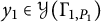 $ y_1\in \mathcal {Y}(\Gamma _{1,P_1})$
,
 $ \mathfrak {h}_5(F_{1,y_1})$
is a fiber of
 $ t(\varphi _{P_1}(y_1))$
. By Lemmas A.5 and A.8, Theorem A.6, and Remark A.7, there is an isotopy
 $\mathfrak {h}_{u}$
(
 $5\leq u\leq 6$
) from
 $\mathfrak {h}_{5}$
such that
 $$ \begin{align*} & \mathfrak{h}_{u}|_{\mathbb T_{1,P_1}}=\mathfrak{h}_{5}|_{\mathbb T_{1,P_1}}, && \mathfrak{h}_{u}|_{\partial\mathscr{B}(\mathcal C_1,P_1)}=\mathfrak{h}_{5}|_{\partial\mathscr{B}(\mathcal C_1,P_1)} \end{align*} $$
for any
 $5\leq u\leq 6$
, and
 $\mathfrak {h}_{6}$
maps every fiber of all
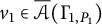 $v_1\in \overline {\mathcal {A}}(\Gamma _{1,P_1})$
to that of
 $\varphi _{P_1}(v_1)$
. Put
 $\mathfrak {g}_{P_1}:=\mathfrak {h}_{6}$
, which satisfies (i)–(iii) and (v). Furthermore, it follows from [Reference Artal Bartolo, Bannai, Shirane and Tokunaga3, Remark 3.5] that
 $\mathfrak {g}_{P_1}$
satisfies (iv).
By identifying
 $ Y_i\setminus \mathcal C_i'$
with
 ${\mathbb {P}}^2\setminus \mathcal C_i$
, let
 $ \mathfrak {m}_{v_i}\in \pi _1({\mathbb {P}}^2\setminus \mathcal C_i)$
be a meridian of
 $ D^{\prime }_{v_i}\subset \mathcal C_i'$
for
 $v_i\in \mathcal {V}(\Gamma _i)$
. Theorem 1.2 follows from the next theorem.
Theorem 3.10 Let
 $\mathcal C_1,\mathcal C_2\subset {\mathbb {P}}^2$
be two plane curves. Assume that there is a homeomorphism
 $h\colon U(\mathcal C_1)\to U(\mathcal C_2)$
with
 $h(\mathcal C_1)=\mathcal C_2$
. Let
 $\varphi \colon \mathrm {Cmb}(\mathcal C_1)\to \mathop {\mathrm {Cmb}}(\mathcal C_2)$
be the equivalence map constructed in Remark 3.3. Then there exists a homeomorphism
 $\Psi _{\mathscr {B}}\colon \mathscr {B}(\mathcal C_1)\to \mathscr {B}(\mathcal C_2)$
such that
-
(i)
$\Psi _{\mathscr {B}}$
is homotopic to the restriction of h in
$U(\mathcal C_2)\setminus \mathcal C_2$
; -
(ii)
$ \Psi _{\mathscr {B}}(T_{y_1})=T_{\varphi (y_1)}$
for each
$y_1\in \mathcal {Y}(\Gamma _1)$
; -
(iii)
$ \Psi _{\mathscr {B}}(M_{v_1})=M_{\varphi (v_1)}$
for each
$v_1\in \mathcal {V}(\Gamma _1)$
; -
(iv) there is
$\alpha \in \{\pm 1\}$
such that
$ \Psi _{\mathscr {B}\ast }(\mathfrak {m}_{v_1})=\mathfrak {m}_{v_2}^\alpha $
up to conjugate for any
$v_i\in \mathcal {V}(\Gamma _i)$
with
$v_2=\varphi (v_1)$
.










In particular,
 $\Psi _{\mathscr {B}\ast }=\Psi _h^\infty $
.
Proof Let
 $h'\colon \mathscr {B}(\mathcal C_1)\to \mathscr {B}(\mathcal C_2)$
be the map constructed in Remark 3.2. For
 $v_1\in \mathrm {Str}_1$
and
 $v_2=\varphi (v_1)$
, since
 $\boldsymbol {e}_1(v_1)=\boldsymbol {e}_2(v_2)$
, we may also assume that
 $h'$
preserves fibers and trivializations of boundary components of
 $ p_{v_i}\colon M_{v_i}\to B_{v_i}$
. By Lemmas 3.4 and 3.9, we obtain a desired homeomorphism
 $\Psi _{\mathscr {B}}\colon \mathscr {B}(\mathcal C_1)\to \mathscr {B}(\mathcal C_2)$
after a certain homotopy near
 $\bigcup _{P_2\in \mathrm {Sing}(\mathcal C_2)}U(P_2)$
.
4 G-combinatorial type of plane curves
In this section, we define G-combinatorial type as a modified plumbing graph together with certain information, which describe the embedded topology of
 ${\phi }^{-1}(\mathcal C)$
in its regular neighborhood for a plane curve
 $\mathcal C\subset {\mathbb {P}}^2$
and the G-cover
 $\phi \colon X\to {\mathbb {P}}^2$
given by a surjection
 $\theta \colon \pi _1({\mathbb {P}}^2\setminus \mathcal C)\to G$
.
Let
 $\mathcal C\subset {\mathbb {P}}^2$
be a plane curve, and let
 $\sigma \colon Y\to {\mathbb {P}}^2$
be the minimal good embedded resolution of
 $\mathcal C$
, and put
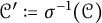 $\mathcal C':=\sigma ^{-1}(\mathcal C)$
. Let
 $ \mathrm {Cmb}(\mathcal C)=(\Gamma _{\mathcal C},\boldsymbol {g}_{\mathcal C},\boldsymbol {e}_{\mathcal C}; \mathrm { Str}_{\mathcal C})$
be the combinatorics of
 $\mathcal C$
, let
 $p_v\colon M_v\to B_v$
and
 $T_y\subset M_{t(y)}$
be the
 $S^1$
-bundle of
 $v\in \mathcal {V}(\Gamma _{\mathcal C})$
and the torus corresponding to
 $y\in \mathcal {Y}(\Gamma _{\mathcal C})$
, respectively, as in the previous section. Let G be a finite group. We assume that there is a surjective homomorphism
 $\theta \colon \pi _1({\mathbb {P}}^2\setminus \mathcal C)\to G$
. Then
 $\theta $
induces the G-covers
 $\phi \colon X\to {\mathbb {P}}^2$
and
 $\tilde {\phi }\colon \widetilde {X}\to Y$
branched along sub-curves of
 $\mathcal C$
and
 $\mathcal C'$
, respectively. The minimal resolution
 $\tilde {\sigma }'\colon \widetilde {X}'\to \widetilde {X}$
is given in the proof of [Reference Laufer24, Proposition 2.2] explicitly. By Stein factorization, there is a morphism
 $\tilde {\sigma }\colon \widetilde {X}\to X$
such that the following diagram is commutative:

Put
 $\widetilde {\mathcal C}:=\tilde {\phi }^{-1}(\mathcal C')\subset \widetilde {X}$
, and
 $\mathscr {B}^\theta (\mathcal C):=\phi ^{-1}(\mathscr {B}(\mathcal C))$
. We call
 $\mathscr {B}^\theta (\mathcal C)$
a boundary manifold of
 $\widetilde {\mathcal C}$
in
 $\widetilde {X}$
. The modified plumbing graph
 $\Gamma _{\mathrm {pg}}^{\mathrm {m}}(\mathcal C,\theta )$
corresponding to
 $\mathscr {B}^\theta (\mathcal C)$
is defined in [Reference Hironaka20], which can be constructed as follows.
It follows from the minimal resolution
 $\tilde {\sigma }'$
that
 $\widetilde {\mathcal C}\subset \widetilde {X}$
consists of just two branches locally at each
 ${P}\in \mathrm {Sing}(\widetilde {\mathcal C})=\tilde {\phi }^{-1}( \mathrm { Sing}(\mathcal C'))$
. Since each irreducible component of
 $\mathcal C'$
is smooth, if
 $D_1\cap D_2\ne \emptyset $
for
 $D_1,D_2\in \mathrm {Irr}(\widetilde {\mathcal C})$
with
 $D_1\ne D_2$
, then
 $\tilde {\phi }(D_1)\ne \tilde {\phi }(D_2)$
. Hence, we can define the dual graph
 $\Gamma _{\mathcal C}^\theta $
of
 $\widetilde {\mathcal C}$
as follows by using an arbitrary total order
 $\prec $
on
 $\mathrm {Irr}(\mathcal C')$
:
-
•
$\mathcal {V}(\Gamma _{\mathcal C}^\theta ):=\left \{v_D \ \middle | \ D\in \mathrm {Irr}\big ( \widetilde {\mathcal C} \big )\right \}$
and
$\mathcal {Y}(\Gamma _{\mathcal C}^\theta ):=\left \{ y_{{P}}, \ \overline {y}_{P} \ \middle | \ {P}\in \mathrm { Sing}(\widetilde {\mathcal C}) \right \}$
, -
• if
${P}\in D_1\cap D_2$
for
$D_1,D_2\in \mathrm {Irr}(\widetilde {\mathcal C})$
with
$ \tilde {\phi }(D_1)\precneqq \tilde {\phi }(D_2)$
, then
$o(y_P):=v_{D_1}$
and
$t(y_P):=v_{D_2}$
.





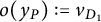

Let
 $i_v\colon M_v\to {\mathbb {P}}^2\setminus \mathcal C$
and
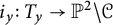 $i_y\colon T_y\to {\mathbb {P}}^2\setminus \mathcal C$
be inclusions for each
 $v\in \mathcal {V}(\Gamma _{\mathcal C})$
and
 $y\in \mathcal {Y}(\Gamma _{\mathcal C})$
, respectively, and put
 $$ \begin{align*} \begin{aligned} G_v&:=\theta\circ {i_v}_\ast\big(\pi_1(M_v)\big), & H_v&:=\theta\circ {i_v}_\ast\Big( \big\langle [F_v] \big\rangle \Big), & G_y&:=\theta\circ {i_y}_\ast\big(\pi_1(T_y)\big) \end{aligned} \end{align*} $$
for each
 $v\in \mathcal {V}(\Gamma _{\mathcal C})$
and
 $y\in \mathcal {Y}(\Gamma _{\mathcal C})$
, where
 $F_v$
is a fiber of
 $p_v$
, and
 $\langle [F_v]\rangle $
is the subgroup of
 $\pi _1(M_v)$
generated by the class
 $[F_v]$
. The subgroups
 $G_v$
,
 $H_v$
, and
 $G_y$
are uniquely determined up to conjugate in G. Since the kernel of
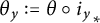 $\theta _y:=\theta \circ {i_y}_\ast $
has a finite index in
 $\pi _1(T_y)\cong \mathbb Z\oplus \mathbb Z$
for each
 $y\in \mathcal {Y}(\Gamma _{\mathcal C})$
, we have
 $\ker \theta _y\cong \mathbb Z\oplus \mathbb Z$
. We take the basis of
 $\pi _1(T_y)$
according to the trivialization
 $\tau _y\colon S^1\times S^1\to T_y$
for each
 $y\in \mathcal {Y}(\Gamma _{\mathcal C})$
. We fix the unique basis of
 $\ker \theta _y\cong \mathbb Z\oplus \mathbb Z$
so that the inclusion
 $\ker \theta _y\to \pi _1(S^1\times S^2)$
induced by
 $\tau _y$
is represent by a matrix
 $$ \begin{align} \boldsymbol{m}_\theta(y):=\begin{pmatrix} c(y) & 0 \\ b(y) & a(y) \end{pmatrix} \end{align} $$
with
 $0\leq b(y)<a(y)$
and
 $c(y)>0$
. We can regard
 $\boldsymbol {m}_\theta $
as a map
 $\boldsymbol {m}_\theta \colon \mathcal {Y}(\Gamma _{\mathcal C})\to \mathrm {Fin}(S^1\times S^1)$
. Since the following diagram is commutative:

 $\boldsymbol {m}_\theta (y)_\ast $
and
 $(J\boldsymbol {m}_\theta (\overline {y}))_\ast $
have the same image in
 $\pi _1(S^1\times S^1)\cong \mathbb Z\oplus \mathbb Z$
. We define
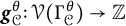 $\boldsymbol {g}_{\mathcal C}^\theta \colon \mathcal {V}(\Gamma _{\mathcal C}^\theta )\to \mathbb Z$
,
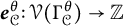 $\boldsymbol {e}_{\mathcal C}^\theta \colon \mathcal {V}(\Gamma _{\mathcal C}^\theta )\to \mathbb Z$
and
 $\boldsymbol {m}_{\mathcal C}^\theta \colon \mathcal {Y}(\Gamma _{\mathcal C}^\theta )\to \mathrm {Fin}(\mathbb Z\times \mathbb Z)$
by
 $$ \begin{align*} \boldsymbol{g}_{\mathcal C}^\theta(w)&:= \frac{1}{2}\left( 2- \frac{\# G_{v}}{\# H_{v}} \Big(2-2\boldsymbol{g}_{\mathcal C}(v)-\boldsymbol{d}(v)\Big) -\sum_{\substack{y\in\mathcal{Y}(\Gamma_{\mathcal C}), \ t(y)=v}} \frac{\# G_{v}}{\# G_y} \right), \\ \boldsymbol{e}_{\mathcal C}^\theta(w)&:=\frac{\# G_v}{(\# H_v)^2} \boldsymbol{e}_{\mathcal C}(v)-\sum_{\substack{y\in\mathcal{Y}(\Gamma_{\mathcal C}), \ t(y)=v}}\frac{b(y)}{a(y)}\frac{ \# G_v}{\#G_y}, \\ \boldsymbol{m}_{\mathcal C}^\theta(z)&:=\boldsymbol{m}_\theta(y) \end{align*} $$
for each
 $w\in \mathcal {V}(\Gamma _{\mathcal C}^\theta )$
and
 $z\in \mathcal {Y}(\Gamma _{\mathcal C}^\theta )$
, where
 $v:=\mathrm {pr}_{\mathcal C}^\theta (w)$
and
 $y:=\mathrm {pr}_{\mathcal C}^\theta (z)$
(see [Reference Hironaka20, Lemmas 8.2 and 9.1]). Since
 $H_v\subset G_v$
for each
 $v\in \mathcal {V}(\Gamma _{\mathcal C})$
, the image of
 $\boldsymbol {g}_{\mathcal C}^\theta $
is in
 $\mathbb Z$
. Note that, for each
 $D\in \mathrm {Irr}(\widetilde {\mathcal C})$
,
 $\boldsymbol {e}_{\mathcal C}^\theta (v_D)$
(resp.
 $\boldsymbol {g}_{\mathcal C}^\theta (v_D)$
) is equal to the self-intersection number (resp. the genus) of the strict transformation
 $D'\subset \widetilde {X}'$
of D. Hence,
 $$\begin{align*}\Gamma^{\mathrm{m}}_{\mathrm{pg}}(\mathcal C,\theta):=(\Gamma_{\mathcal C}^\theta,\boldsymbol{g}_{\mathcal C}^\theta,\boldsymbol{e}_{\mathcal C}^\theta,\boldsymbol{m}_{\mathcal C}^\theta) \end{align*}$$
is a modified plumbing graph. By [Reference Hironaka20, Section 5],
 $\mathscr {B}^\theta (\mathcal C)$
with the graph structure
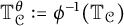 $\mathbb T_{\mathcal C}^\theta :=\phi ^{-1}(\mathbb T_{\mathcal C})$
is the plumbed manifold
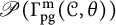 $\mathscr {P}(\Gamma _{\mathrm {pg}}^{\mathrm {m}}(\mathcal C,\theta ))$
.
Remark 4.1
 $\Gamma _{\mathrm {pg}}^{\mathrm {m}}(\mathcal C,\theta )$
can be constructed from the algebraic data of
 $\tilde {\phi }\colon \widetilde {X}\to Y$
and
 $\widetilde {\mathcal C}':=(\tilde {\sigma }')^{-1}(\widetilde {\mathcal C})$
in the minimal resolution
 $\widetilde {X}'$
as follows.
The graph
 $\Gamma _{\mathcal C}^\theta $
is obtained from the dual graph
 $\widetilde {\Gamma }_{\mathcal C}'$
of
 $\widetilde {\mathcal C}'$
by contracting all vertices corresponding to the exceptional divisors of
 $\tilde {\sigma }'$
. The maps
 $\boldsymbol {e}_{\mathcal C}^\theta $
and
 $\boldsymbol {g}_{\mathcal C}^\theta $
are induced by the self-intersection numbers and the genera on
 $\widetilde {\Gamma }_{\mathcal C}'$
as mentioned above.
For
 $y\in \mathcal {Y}(\Gamma _{\mathcal C}^\theta )$
,
 $\boldsymbol {m}_{\mathcal C}^\theta (y)$
is described as follows. For
 $v\in \mathcal {V}(\Gamma _{\mathcal C}^\theta )$
, let
 $\omega _v\in \mathbb Z_{>0}$
be the ramification index of
 $\tilde {\phi }$
at the component of
 $\widetilde {\mathcal C}\subset \widetilde {X}$
corresponding to v. We may assume by [Reference Laufer24] that the contracted part in
 $\widetilde {\Gamma }_{\mathcal C} '$
over y is the following tree:

for
 $k_i\geq 2$
for
 $i=1,\dots ,s$
, where
 $t(y)',o(y)'\in \mathcal {V}(\widetilde {\Gamma }_{\mathcal C}')$
are the vertices corresponding to
 $t(y),o(y)\in \mathcal {V}(\Gamma _{\mathcal C}^\theta )$
, respectively. Let
 $\alpha _y,\beta _y\in \mathbb Z$
be coprime integers satisfying
 $\beta _y\ne 0$
and
 $$\begin{align*}\frac{\alpha_y}{\beta_y}=[k_1,k_2,\dots,k_s], \end{align*}$$
where
 $[k_1,\dots ,k_s]$
is the continuous fraction defined in [Reference Neumann28, p. 318]. Then we can check from the proof of [Reference Laufer24, Proposition 2.2] that
 $\boldsymbol {m}_{\mathcal C}^\theta (y)$
is the matrix in (4.1) with
 $a(y)=\omega _{o(y)}\alpha _y$
,
 $b(y)=\omega _{o(y)}\beta _y$
and
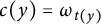 $c(y)=\omega _{t(y)}$
.
The G-cover
 $\tilde {\phi }\colon \widetilde {X}\to Y$
induces the map
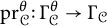 $\mathrm {pr}_{\mathcal C}^\theta \colon \Gamma _{\mathcal C}^\theta \to \Gamma _{\mathcal C}$
defined by
 $$\begin{align*}\mathrm{pr}_{\mathcal C}^\theta(v_D):=v_{\tilde{\phi}(D)} ,\qquad \mathrm{pr}_{\mathcal C}^\theta(y_P):=y_{\tilde{\phi}(P)}, \qquad \mathrm{pr}_{\mathcal C}^\theta(\overline{y_P}):=\overline{y_{\tilde{\phi}(P)}} \end{align*}$$
for each
 $D\in \mathrm {Irr}(\widetilde {\mathcal C})$
and
 $P\in \mathrm {Sing}(\widetilde {\mathcal C})$
, where
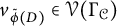 $v_{\tilde {\phi }(D)}\in \mathcal {V}(\Gamma _{\mathcal C})$
and
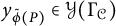 $y_{\tilde {\phi }(P)}\in \mathcal {Y}(\Gamma _{\mathcal C})$
are the vertex and the edge corresponding to
 $\tilde {\phi }(D)\in \mathrm {Irr}(\mathcal C')$
and
 $\tilde {\phi }(P)\in \mathrm { Sing}(\mathcal C')$
, respectively, such that
 $$\begin{align*}o(\mathrm{pr}_{\mathcal C}^\theta(y_P))=\mathrm{pr}_{\mathcal C}^\theta(o(y_P)), \qquad t(\mathrm{pr}_{\mathcal C}^\theta(y_P))=\mathrm{pr}_{\mathcal C}^\theta(t(y_P)). \end{align*}$$
Moreover, the action of G on
 $\widetilde {X}$
induces the action
 $\rho _{\mathcal C}^\theta \colon G\times \Gamma _{\mathcal C}^\theta \to \Gamma _{\mathcal C}^\theta $
defined by
 $$\begin{align*}\rho_{\mathcal C}^\theta(g,v_D):=v_{g{\cdot}D}, \qquad \rho_{\mathcal C}^\theta(g,y_P):=y_{g{\cdot}P}, \qquad \rho_{\mathcal C}^\theta(g,\overline{y_P}):=\overline{y_{g{\cdot}P}} \end{align*}$$
for each
 $g\in G$
,
 $D\in \mathrm {Irr}(\widetilde {\mathcal C}),$
and
 $P\in \mathrm {Sing}(\widetilde {\mathcal C})$
.
Definition 4.2 With the above notation, we define the G-combinatorial type (or the G-combinatorics for short)
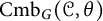 $ \mathrm { Cmb}_G(\mathcal C,\theta )$
of
 $\mathcal C$
with respect to
 $\theta $
as the following
 $6$
-tuple:
 $$ \begin{align} \mathrm{Cmb}_G(\mathcal C,\theta):=(\Gamma_{\mathcal C} ^\theta, \boldsymbol{g}_{\mathcal C}^\theta, \boldsymbol{e}_{\mathcal C}^\theta, \boldsymbol{m}_{\mathcal C}^\theta; \rho_{\mathcal C}^\theta,\mathrm{pr}_{\mathcal C}^\theta). \end{align} $$
For simplicity, let
 $g{\cdot } \bullet $
denote
 $\rho _{\mathcal C}^\theta (g, \bullet )$
for each
 $g\in G$
and
 $\bullet \in \mathcal {V}(\Gamma _{\mathcal C}^\theta )\cup \mathcal {Y}(\Gamma _{\mathcal C}^\theta )$
.
For each
 $w\in \mathcal {V}(\Gamma _{\mathcal C}^\theta )$
, let
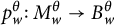 $p_w^\theta \colon M_w^\theta \to B_w^\theta $
denote the
 $S^1$
-bundle of w, where
 $M_w^\theta $
is a closed subset of
 $\mathscr {B}^\theta (\mathcal C)$
. For each
 $z\in \mathcal {Y}(\Gamma _{\mathcal C}^\theta )$
, let
 $T_z^\theta \subset M_{t(z)}^\theta $
be the boundary component of
 $M_{t(z)}^\theta $
corresponding to z. By the definition of
 $\mathrm {pr}_{\mathcal C}^\theta $
and
 $\rho _{\mathcal C}^\theta $
, we have
 $$ \begin{align*} \tilde{\phi}(M_w^\theta)&=M_v\subset\mathscr{B}(\mathcal C), & \tilde{\phi}(T_z^\theta)&=T_y\subset M_{t(y)}, & g{\cdot}M_w^\theta &=M_{g{\cdot}w}^\theta, & g{\cdot}T_z^\theta &=T_{g{\cdot}z}^\theta \end{align*} $$
for each
 $w\in \mathcal {V}(\Gamma _{\mathcal C}^\theta )$
and
 $z\in \mathcal {Y}(\Gamma _{\mathcal C}^\theta )$
, where
 $v:=\mathrm {pr}_{\mathcal C}^\theta (w)$
and
 $y:=\mathrm {pr}_{\mathcal C}^\theta (z)$
.
For two plane curves
 $\mathcal C_i$
with surjections
 $\theta _i\colon \pi _1({\mathbb {P}}^2\setminus \mathcal C_i)\to G$
(
 $i=1,2$
), we describe
 $ \mathrm {Cmb}_G(\mathcal C_i,\theta _i)$
by
 $ \mathrm {Cmb}_G(\mathcal C_i,\theta _i)=(\Gamma _i^{\theta },\boldsymbol {g}_i^{\theta }, \boldsymbol {e}_i^\theta , \boldsymbol {m}_i^\theta; \rho _{i}^\theta , \mathrm {pr}_i^\theta )$
.
Definition 4.3 For two plane curves
 $\mathcal C_i$
with surjections
 $\theta _i\colon \pi _1({\mathbb {P}}^2\setminus \mathcal C_i)\to G$
and an equivalence map
 $\varphi \colon \mathrm {Cmb}(\mathcal C_1)\to \mathrm {Cmb}(\mathcal C_2)$
, a G-equivalence map
 $\varphi _G^\theta \colon \mathop {\mathrm {Cmb}}_G(\mathcal C_1,\theta _1)\to \mathop {\mathrm {Cmb}}_G(\mathcal C_2,\theta _2)$
with respect to
 $\varphi $
is an isomorphism
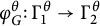 $\varphi _G^\theta \colon \Gamma _{1}^{\theta }\to \Gamma _{2}^{\theta }$
of graphs such that
-
•
$\boldsymbol {g}_{1}^{\theta }=\boldsymbol {g}_{2}^{\theta }\circ \varphi _G^\theta $
,
$\boldsymbol {e}_{1}^{\theta }=\boldsymbol {e}_{2}^{\theta }\circ \varphi _G^\theta $
,
$\boldsymbol {m}_{1}^{\theta }=\boldsymbol {m}_{2}^{\theta }\circ \varphi _G^\theta $
, -
• there is an automorphism
$\tau \colon G\to G$
such that for each
$$\begin{align*}\varphi_G^\theta(g{\cdot}w)=\tau(g){\cdot}\varphi_G^\theta(w), \qquad \varphi_G^\theta(g{\cdot}z)=\tau(g){\cdot}\varphi_G^\theta(z)\end{align*}$$
$w\in \mathcal {V}(\Gamma _{1}^{\theta })$
and
$z\in \mathcal {Y}(\Gamma _{1}^{\theta })$
,
-
•
$\varphi \circ \mathrm {pr}_{1}^{\theta }=\mathrm {pr}_{2}^{\theta }\circ \varphi _G^\theta $
.
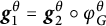
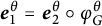
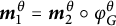




Theorem 4.4 Let
 $\mathcal C_i\subset {\mathbb {P}}^2$
be two plane curves with surjections
 $\theta _i\colon \pi _1({\mathbb {P}}^2\setminus \mathcal C_i)\to G$
. Assume that there are a homeomorphism
 $h\colon {\mathbb {P}}^2\to {\mathbb {P}}^2$
and an automorphism
 $\tau \colon G\to G$
such that
 $h(\mathcal C_1)=\mathcal C_2$
and
 $\tau \circ \theta _1=\theta _2\circ h_\ast $
. Let
 $\varphi \colon \mathrm {Cmb}(\mathcal C_1)\to \mathop {\mathrm {Cmb}}(\mathcal C_2)$
be the equivalence map induced by h. Then there is a G-equivalence map
 $\varphi _G^\theta \colon \mathrm {Cmb}_G(\mathcal C_1,\theta _1)\to \mathrm { Cmb}_G(\mathcal C_2,\theta _2)$
with respect to
 $\varphi $
.

Proof Let
 $\sigma _i\colon Y_i\to {\mathbb {P}}^2$
be the minimal good embedded resolution of
 $\mathcal C_i$
, and put
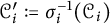 $\mathcal C^{\prime }_{i}:=\sigma _i^{-1}(\mathcal C_i)$
. We identify
 $Y_i\setminus \mathcal C_i'$
with
 ${\mathbb {P}}^2\setminus \mathcal C_i$
via
 $\sigma _i$
. Let
 $\tilde {\phi }_i\colon \widetilde {X}_i\to Y_i$
be the G-covers induced by
 $\theta _i$
for
 $i=1,2$
, and put
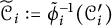 $\widetilde {\mathcal C}_{i}:=\tilde {\phi }_i^{-1}(\mathcal C^{\prime }_{i})$
. Let
 $\iota _i'\colon \mathscr {B}(\mathcal C_i)\to Y_i\setminus \mathcal C^{\prime }_i$
be the inclusion map, and let
 $\Psi _{\mathscr {B}}\colon \mathscr {B}(\mathcal C_1)\to \mathscr {B}(\mathcal C_2)$
be the homeomorphism constructed from h by Theorem 3.10. By (i) in Theorem 3.10, we have
 $\iota ^{\prime }_{2\ast }\circ \Psi _{\mathscr {B}\ast }=h_\ast \circ \iota ^{\prime }_{1\ast }$
.

Hence this commutative diagram induces a homeomorphism
 $\Psi ^\theta _{\mathscr {B}}\colon \mathscr {B}^\theta (\mathcal C_1)\to \mathscr {B}^\theta (\mathcal C_2)$
such that
 $\tilde {\phi }_2\circ \Psi ^\theta _{\mathscr {B}}=\Psi _{\mathscr {B}}\circ \tilde {\phi }_1$
and
 $\Psi _{\mathscr {B}}^\theta (g\cdot P)=\tau (g)\cdot \Psi ^\theta _{\mathscr {B}}(P)$
for any
 $P\in \mathscr {B}^\theta (\mathcal C_1)$
and
 $g\in G$
(cf. [Reference Shirane35, Theorem 3.4]). By (ii) in Theorem 3.10, we have
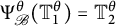 $\Psi _{\mathscr {B}}^\theta (\mathbb T_1^\theta )=\mathbb T_2^\theta $
, where
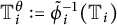 $\mathbb T_i^\theta :=\tilde {\phi }_i^{-1}(\mathbb T_i)$
is the graph structure of
 $\mathscr {B}^\theta (\mathcal C_i)$
with respect to
 $\Gamma _{\mathrm {pg}}^{\mathrm {m}}(\mathcal C_i,\theta _i)$
. Thus,
 $\Psi _{\mathscr {B}}^\theta $
induces an isomorphism
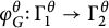 $\varphi ^\theta _G\colon \Gamma _1^\theta \to \Gamma _2^\theta $
such that
-
•
$ \Psi _{\mathscr {B}}^\theta (M_{w_1}^\theta )=M_{w_2}^\theta $
for each
$w_1\in \mathcal {V}(\Gamma _1^\theta )$
and
$w_2:=\varphi _G^\theta (w_1)$
; -
•
$ \Psi _{\mathscr {B}}^\theta (T_{z_1}^\theta )=T^\theta _{z_2}$
for each
$z_1\in \mathcal {Y}(\Gamma _{1}^\theta )$
and
$z_2:=\varphi _G^\theta (z_1)$
; -
•
$\varphi ^\theta _G(g{\cdot }w_1)=\tau (g){\cdot }\varphi _G^\theta (w_1)$
and
$\varphi ^\theta _G(g{\cdot }z_1)=\tau (g){\cdot }\varphi _G^\theta (z_1)$
for each
$g\in G$
,
$w_1\in \mathcal {V}(\Gamma _1^\theta )$
and
$z_1\in \mathcal {Y}(\Gamma _1^\theta )$
; -
•
$\varphi \circ \mathrm {pr}_1^\theta =\mathrm {pr}_2^\theta \circ \varphi _G^\theta $
.


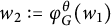
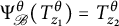

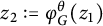





Since the trivialization
 $ \tau _{y_i}$
of
 $ T_{y_i}\subset M_{t(y_i)}$
is determined by meridians
 $ \mathfrak {m}_{t(y_i)}$
and
 $ \mathfrak {m}_{o(y_i)}$
for each
 $y_i\in \mathcal {Y}(\Gamma _i)$
, it follows from (iv) in Theorem 3.10 that
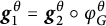 $\boldsymbol {g}^\theta _1=\boldsymbol {g}_2^\theta \circ \varphi _G^\theta $
,
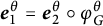 $\boldsymbol {e}_1^\theta =\boldsymbol {e}_2^\theta \circ \varphi _G^\theta $
, and
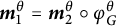 $\boldsymbol {m}_1^\theta =\boldsymbol {m}_2^\theta \circ \varphi _G^\theta $
. Therefore,
 $\varphi _G^\theta $
is a G-equivalence map with respect to
 $\varphi $
.
Remark 4.5 With the same notation in Theorem 4.4, we may assume that the automorphism
 $\tau \colon G\to G$
is the identity map of G by replacing the surjection
 $\theta _2\colon \pi _1({\mathbb {P}}^2\setminus \mathcal C_2)\to G$
with
 $\tau ^{-1}\circ \theta _2$
, which does not change
 $ \mathrm { Cmb}_G(\mathcal C_2,\theta _2)$
except for the action
 $\rho _{2}^\theta $
.
Remark 4.6 Let
 $\mathcal C\subset {\mathbb {P}}^2$
be a plane curve. Let
 $\theta \colon \pi _1({\mathbb {P}}^2\setminus \mathcal C)\to G$
be a surjection, and let
 $\phi \colon X\to {\mathbb {P}}^2$
be the G-cover induced by
 $\theta $
. Let
 $\sigma \colon Y\to {\mathbb {P}}^2$
be the minimal good embedded resolution of
 $\mathcal C$
. If there is a composition of (minimal) blowing-ups
 $\sigma "\colon Y"\to Y$
such that the
 $\mathbb C(X)$
-normalization
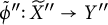 $\tilde {\phi }"\colon \widetilde {X}"\to {Y"}$
is a G-cover with
 $\widetilde {X}"$
smooth, we may define a G-combinatorics
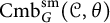 $ \mathrm {Cmb}_G^{\mathrm {sm}}(\mathcal C,\theta )$
as the plumbing graph
 $$\begin{align*}\mathrm{Cmb}_{G}^{\mathrm{sm}}(\mathcal C,\theta)=(\widetilde{\Gamma}_{\mathcal C}^\theta,\tilde{\boldsymbol{e}}_{\mathcal C}^\theta,\tilde{\boldsymbol{g}}_{\mathcal C}^\theta;\tilde{\rho}_{\mathcal C}^\theta, \tilde{\mathrm{pr}}_{\mathcal C}^\theta) \end{align*}$$
together with maps
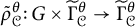 $\tilde {\rho }_{\mathcal C}^\theta \colon G\times \widetilde {\Gamma }_{\mathcal C}^\theta \to \widetilde {\Gamma }_{\mathcal C}^\theta $
and
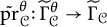 $\tilde {\mathrm {pr}}_{\mathcal C}^\theta \colon \widetilde {\Gamma }_{\mathcal C}^\theta \to \widetilde {\Gamma }_{\mathcal C}$
, where
 $\tilde {\rho }_{\mathcal C}^\theta $
is induced by the action
 $G\curvearrowright \widetilde {X}"$
,
 $\widetilde {\Gamma }_{\mathcal C}$
is the plumbing graph together with the marking
 $\widetilde { \mathrm {Str}}_{\mathcal C}$
of the strict transformations of components of
 $\mathcal C$
, which is constructed from
 $\Gamma _{\mathcal C}$
by blowing-ups (R
 $1^+$
) corresponding to
 $\tilde \sigma "$
, and
 $\tilde {\mathrm {pr}}_{\mathcal C}^\theta $
is the projection induced by
 $\tilde {\phi }$
. By the same argument, we can check that Theorem 4.4 holds for the above G-combinatorics.
If G is a subgroup of the symmetric group of degree
 $3$
, the above assumption is always true by [Reference Horikawa23, Section 2] for
 $\# G=2$
and [Reference Tan36, Theorem 4.1] for
 $\# G=3,6$
.
5 Splitting invariants and G-combinatorics
In this section, we show relation between G-combinatorics and splitting invariants, namely, splitting type [Reference Bannai12], splitting number [Reference Shirane33], connected number [Reference Shirane34], and splitting graph [Reference Shirane35]. For this aim, we define a G-subcombinatorics of a plane curve and its subcurve which has no common component with the branch locus.
Let
 $\mathcal C\subset {\mathbb {P}}^2$
be a plane curve, and let G be a finite group. Assume that there is a surjection
 $\theta \colon \pi _1({\mathbb {P}}^2\setminus \mathcal C)\to G$
. Let
 $\sigma \colon Y\to {\mathbb {P}}^2$
be the minimal good embedded resolution of
 $\mathcal C$
. Let
 $\phi \colon X\to {\mathbb {P}}^2$
and
 $\tilde \phi \colon \widetilde {X}\to Y$
be G-covers induced by
 $\theta $
, and let
 $\Delta _{\phi }\subset {\mathbb {P}}^2$
and
 $\Delta _{\tilde \phi }\subset Y$
be the branch locus of
 $\phi $
and
 $\tilde \phi $
, respectively.
For a subcurve
 $\mathcal C_0\subset \mathcal C$
which has no common component with
 $\Delta _{\phi }$
, let
 $\Gamma _{\mathcal C}(\mathcal C_0)$
be the subgraph of
 $\Gamma _{\mathcal C}$
such that
-
(i)
$\mathcal {V}(\Gamma _{\mathcal C}(\mathcal C_0)):=\left \{ v\in \mathcal {V}(\Gamma _{\mathcal C}) \mid \sigma ({ D_v})\subset \mathcal C_0, \ \sigma ({ D_v})\not \subset \Delta _{\phi } \right \}$
, the set of vertices of
$\Gamma _{\mathcal C}$
corresponding to components of
$\mathcal C_0$
and exceptional divisors over the singularities of
$\mathcal C_0$
outside of
$\Delta _{\phi }$
; -
(ii)
$\mathcal {Y}(\Gamma _{\mathcal C}(\mathcal C_0)):=\left \{ y\in \mathcal {Y}(\Gamma _{\mathcal C}) \mid o(y), t(y)\in \mathcal {V}(\Gamma _{\mathcal C}(\mathcal C_0)) \right \}$
, in other words,
$\Gamma _{\mathcal C}(\mathcal C_0)$
is a full subgraph of
$\Gamma _{\mathcal C}$
.






Put
 $ \mathrm {Str}_{\mathcal C}(\mathcal C_0):=\{v\in \mathrm {Str}_{\mathcal C}\mid { D_v}\subset \mathcal C_0\}$
. Let
 $\Gamma _{\mathcal C}^\theta (\mathcal C_0)$
be the pull-back of
 $\Gamma _{\mathcal C}(\mathcal C_0)$
by
 $\mathrm {pr}_{\mathcal C}^\theta $
,
 $$\begin{align*}\Gamma_{\mathcal C}^\theta(\mathcal C_0) := (\mathrm{pr}_{\mathcal C}^\theta)^{-1}(\Gamma_{\mathcal C}(\mathcal C_0)). \end{align*}$$
Put
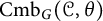 $ \mathrm {Cmb}_G(\mathcal C,\theta )$
as in (4.2). The G-subcombinatorics
 $ \mathrm {Cmb}_G(\mathcal C,\theta ;\mathcal C_0)$
of
 $\mathcal C_0\subset \mathcal C$
is the
 $6$
-tuple
 $$\begin{align*}\mathrm{Cmb}_G(\mathcal C,\theta;\mathcal C_0):=\left(\Gamma_{\mathcal C}^\theta(\mathcal C_0), \boldsymbol{g}_{\mathcal C}^\theta,\boldsymbol{e}_{\mathcal C}^\theta,\boldsymbol{m}_{\mathcal C}^\theta; \rho_{\mathcal C}^\theta, \mathrm{pr}_{\mathcal C}^\theta\right), \end{align*}$$
where, by abuse of notation, the restrictions of
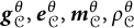 $\boldsymbol {g}_{\mathcal C}^\theta , \boldsymbol {e}_{\mathcal C}^\theta , \boldsymbol {m}_{\mathcal C}^\theta , \rho _{\mathcal C}^\theta $
, and
 $\mathrm {pr}_{\mathcal C}^\theta $
to
 $\Gamma _{\mathcal C}^\theta (\mathcal C_0)$
are denoted by the same symbols. A splitting curve
 ${ D}\subset {\mathbb {P}}^2$
for a G-cover
 $\phi \colon X\to {\mathbb {P}}^2$
is an irreducible curve
 ${ D}\subset {\mathbb {P}}^2$
such that
 ${ D}\not \subset \Delta _{\phi }$
and
 ${\phi }^{-1}(D)$
is not irreducible.
The known invariants can be computed by the G-subcombinatorics as follows:
-
(i) Suppose that
$G=\mathbb Z/2\mathbb Z$
and a subcurve
$\mathcal C_0\subset \mathcal C$
consists of two splitting curves
$ D_1$
and
$ D_2$
with
$ D_1\cap D_2\cap \Delta _{\phi }=\emptyset $
, say
$ {\phi }^\ast D_i=D_i^++D_i^-$
. The splitting type of
$ (D_1,D_2;\Delta _{\phi })$
is the pair of intersection numbers
$ (m_1,m_2)=(D_1^+\cdot D_2^+, D_1^+\cdot D_2^-)$
. Then the splitting type can be computed from
$ \mathrm {Cmb}_G(\mathcal C,\theta; \mathcal C_0)$
by contracting vertices of
$\mathcal {V}(\Gamma _{\mathcal C}^\theta (\mathcal C_0))\setminus {\mathrm {pr}_{\mathcal C}^\theta }^{-1}( \mathrm {Str}_{\mathcal C}(\mathcal C_0))$
. -
(ii) Suppose that
$\mathcal C_0\subset \mathcal C$
is an irreducible component such that
$\mathcal C_0\not \subset \Delta _{\phi }$
. The splitting number
$s_{\phi }(\mathcal C_0)$
is the number of irreducible components of
${\phi }^\ast (\mathcal C_0)$
. Then
$s_{\phi }(\mathcal C)$
is equal to the number of vertices
$w\in \mathcal {V}(\Gamma _{\mathcal C}(\mathcal C_0))$
with
$\mathrm {pr}_{\mathcal C}^\theta (w)\in \mathrm {Str}_{\mathcal C}(\mathcal C_0)$
. -
(iii) Suppose that
$\mathcal C_0=\mathcal C-\Delta _{\phi }$
as reduced divisors on
${\mathbb {P}}^2$
. The connected number
$c_{\phi }(\mathcal C_0)$
is the number of connected components of
${\phi }^{-1}(\mathcal C_0\setminus \Delta _{\phi })$
. Then
$c_{\phi }(\mathcal C_0)$
is equal to the number of connected components of
$\Gamma _{\mathcal C}^\theta (\mathcal C_0)$
. -
(iv) With the same assumption of (iii), the splitting graph of
$\mathcal C_0$
is the bipartite graph
$\mathcal {S}_{\phi ,\mathcal C_0}$
together with action of G whose vertices corresponding to irreducible components of
${\phi }^{-1}(\mathcal C_0)$
and singular points of
${\phi }^{-1}(\mathcal C_0\setminus \Delta _{\phi })$
, and
$\mathcal {S}_{\phi ,\mathcal C_0}$
describes configuration of components of
${\phi }^{-1}(\mathcal C_0\setminus \Delta _{\phi })$
(see [Reference Shirane35] for details). Put
$ \mathrm {Str}_{\mathcal C}^\theta :=(\mathrm {pr}_{\mathcal C}^\theta )^{-1}( \mathrm { Str}_{\mathcal C})$
. To construct the splitting graph from
$\Gamma _{\mathcal C}^\theta (\mathcal C_0)$
, let
$\Gamma _0$
be the full subgraph of
$\Gamma _{\mathcal C}^\theta (\mathcal C_0)$
whose vertex set is
$\mathcal {V}(\Gamma _{\mathcal C}^\theta (\mathcal C_0))\setminus \mathrm {Str}^\theta _{\mathcal C}$
. Let
$\mathcal {Y}^\theta _{\mathcal C_0}$
be the set of edges
$z\in \mathcal {Y}(\Gamma _{\mathcal C}^\theta (\mathcal C_0))$
such that
$o(z),t(z)\in \mathrm {Str}_{\mathcal C}^\theta $
. Note that the disjoint union
$\mathrm {Conn}(\Gamma _0)\sqcup \mathcal {Y}^\theta _{\mathcal C_0}$
corresponds to the set of singularities of
${\phi }^{-1}(\mathcal C_0)$
outside
${\phi }^{-1}(\Delta _{\phi })$
, where
$\mathrm {Conn}(\Gamma _0)$
is the set of connected components of
$\Gamma _0$
. Then
$\mathcal {S}:=\mathcal {S}_{\phi ,\mathcal C_0}$
is obtained from
$\Gamma _{\mathcal C}^\theta (\mathcal C_0)$
as follows:-
(4a) The vertex set
$\mathcal {V}(\mathcal {S})$
consists of the following two parts
$\mathcal {V}_1(\mathcal {S})$
and
$\mathcal {V}_2(\mathcal {S})$
:
$$ \begin{align*} \mathcal{V}_1(\mathcal{S})&:=\mathcal{V}(\Gamma_{\mathcal C}^\theta(\mathcal C_0))\cap \mathrm{ Str}^\theta_{\mathcal C}, & \mathcal{V}_2(\mathcal{S})&:=\{w_k\mid k\in \mathrm{Conn}(\Gamma_0)\sqcup\mathcal{Y}_{\mathcal C_0}^\theta\}; \end{align*} $$
-
(4b) for
$v\in \mathcal {V}_1(\mathcal {S})$
and
$w_k\in \mathcal {V}_2(\mathcal {S})$
with
$k\in \mathrm {Conn}(\Gamma _0)\sqcup \mathcal {Y}_{\mathcal C_0}^\theta $
, there is an edge
$y_{v,w_k}$
with
$o(y_{v,w_k})=v$
and
$t(y_{v,w_k})=w_k$
if and only if there is an edge
$y\in \mathcal {Y}(\Gamma _{\mathcal C}^\theta (\mathcal C_0))$
satisfying one of the following conditions:-
(i)
$k\in \mathcal {Y}_{\mathcal C_0}^\theta $
,
$t(y)=v$
and
$y=k$
; -
(ii)
$k\in \mathrm {Conn}(\mathcal C_0)$
,
$t(y)=v$
and
$o(y)\in k$
;
-
-
(4c) the action of G on
$\mathcal {S}$
is induced from the action
$\rho _{\mathcal C}^\theta $
of G on
$\Gamma _{\mathcal C}^\theta (\mathcal C_0)$
.
-




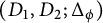














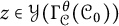

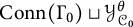




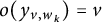

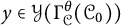





In particular, if two plane curves
 $\mathcal C_i\subset {\mathbb {P}}^2$
(
 $i=1,2$
) with surjections
 $\theta _i\colon \pi _1({\mathbb {P}}^2\setminus \mathcal C_i)\to G$
have different splitting invariants (splitting types, splitting numbers, connected numbers, or splitting graphs), then they have different G-combinatorics with respect to
 $\theta _i$
.
Remark 5.1 For each
 $i=1,2$
, let
 $\mathcal B_i\subset {\mathbb {P}}^2$
be a plane curve of even degree, let
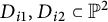 $ D_{i1}, D_{i2}\subset {\mathbb {P}}^2$
be distinct two irreducible curves with
 $ D_{ij}\not \subset \mathcal B_i$
for
 $j=1,2$
and
 $ D_{i1}\cap D_{i2}\cap \mathcal B_i=\emptyset $
, and let
 $\phi _i\colon X_i\to {\mathbb {P}}^2$
be the double cover branched along
 $\mathcal B_i$
. In [Reference Bannai12], it was proved under the assumption
 $C_{i1}\pitchfork C_{i2}$
for
 $i=1,2$
that, if
 $(C_{11},C_{12};\mathcal B_1)$
and
 $(C_{21},C_{22};\mathcal B_2)$
have distinct splitting types, then there is no homeomorphism
 $h\colon {\mathbb {P}}^2\to {\mathbb {P}}^2$
such that
 $h(C_{11}+C_{12})=C_{21}+C_{22}$
and
 $h(\mathcal B_1)=\mathcal B_2$
, where
 $C_{i1}\pitchfork C_{i2}$
means that
 $C_{i1}$
and
 $C_{i2}$
intersect transversally. By [Reference Brieskorn and Knörrer13, III, Theorem 21], this statement holds even if we omit the assumption
 $C_{i1}\pitchfork C_{i2}$
.
6 Quasi-triangular curves
In this section, we consider a generalization of triangular curves studied in [Reference Artal Bartolo, Cogolludo-Agustín and Morales7], which is related with Artal arrangements studied in [Reference Shirane35].
Definition 6.1 Let
 $d>1$
be an integer, and let
 $ D\subset {\mathbb {P}}^2$
be a plane curve of degree
 $2d$
, and let
 $L_1,L_2,L_3\subset {\mathbb {P}}^2$
be three lines.
-
(i) For a partition
$\mathfrak {p}:=(e_1,\dots ,e_n)$
of d, we call a singularity
$P\in { D}$
a multi-cusp of type
$\mathfrak {p}$
if the local topological type of
$ D$
at P is given by
$$\begin{align*}\prod_{i=1}^n\left((x+iy)^{e_i}+y^{e_i+1}\right)=0. \end{align*}$$
-
(ii) For three partitions
$\mathfrak {p}_1,\mathfrak {p}_2,\mathfrak {p}_3$
of d, we call
${ D}+L_1+L_2+L_3$
a quasi-triangular curve of type
$(\mathfrak {p}_1,\mathfrak {p}_2,\mathfrak {p}_3)$
if
$ \mathrm { Sing}(D)$
consists of three multi-cusps
$P_i$
of type
$\mathfrak {p}_i$
(
$i=1,2,3$
) and
$L_i$
passes through
$P_j$
and
$P_k$
for
$\{i,j,k\}=\{1,2,3\}$
.







Remark 6.2 Let
 $\mathfrak {p}_1,\mathfrak {p}_2,\mathfrak {p}_3$
be three partitions of
 $d>1$
, and let
 $\mathcal C={ D}+L_1+L_2+L_3$
be a quasi-triangular curve of type
 $(\mathfrak {p}_1,\mathfrak {p}_2,\mathfrak {p}_3)$
.
-
(i) Since
${ D}\cdot L_i=2d$
,
${ D}\cap L_i$
consists of two singular points
$P_j, P_k$
of
$ D$
, and
$L_i$
is not tangent to
$ D$
at
$P_j$
and
$P_k$
. -
(ii) We obtain an Artal arrangement
$\overline { D}+L_1'+L_2'+L_3'$
of type
$(\mathfrak {p}_1,\mathfrak {p}_2,\mathfrak {p}_3)$
after a quadratic transformation, that is, blowing-up at
$P_1,P_2,P_3$
and blowing-down of the strict transformations of
$L_1,L_2,L_3$
. Since
$\overline { D}$
is smooth and birational to
$ D$
,
$ D$
is irreducible. In particular, the combinatorics of a quasi-triangular curve is determined by its type
$(\mathfrak {p}_1,\mathfrak {p}_2,\mathfrak {p}_3)$
.





We fix three partitions
 $\mathfrak {p}_i=(e_{i,1},\dots ,e_{i,n_i})$
of
 $d>1$
for
 $i=1,2,3$
, and put
 $\mathfrak {P}:=(\mathfrak {p}_1,\mathfrak {p}_2,\mathfrak {p}_3)$
. Let
 $s_i$
be the greatest common divisor
 $\gcd (e_{i,1},\dots ,e_{i,n_i})$
for
 $i=1,2,3$
, and put
 $s:=\gcd (s_1,s_2,s_3)$
. Let
 $\widetilde {\Sigma }_{\mathfrak {P}}$
be the realization space of quasi-triangular curves of type
 $\mathfrak {P}$
.
Lemma 6.3 Let
 $\mathcal C:={ D}+\mathcal {L}$
be a quasi-triangular curve of type
 $\mathfrak {P}=(\mathfrak {p}_1,\mathfrak {p}_2,\mathfrak {p}_3)$
, where
 $\mathcal {L}:=L_1+L_2+L_3$
. Put
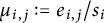 $\mu _{i,j}:=e_{i,j}/s_i$
. Then, after a certain projective transform of
 ${\mathbb {P}}^2$
,
 $\mathcal {L}$
defined by
 $xyz=0$
, and
 $ D$
is defined by
 $\overline {F}_{\mathfrak {P}}(\beta ,\{c_{i,j}\},g_0)=0$
with
 $$ \begin{align*} \overline{F}_{\mathfrak{P}}(\beta,\{c_{i,j}\},g_0) :=\ &x^d\prod_{j=1}^{n_1}(z+c_{1,j}y)^{e_{1,j}}+y^d\prod_{j=1}^{n_2}(x+c_{2,j}z)^{e_{2,j}}+z^d\prod_{j=1}^{n_3}(y+c_{3,j}x)^{e_{3,j}} \\ & \quad-y^dz^d-z^dx^d-x^dy^d+x^2y^2z^2g_0(yz,zx,xy), \notag \end{align*} $$
where
 $\beta $
is an integer with
 $0\leq \beta <s$
,
 $g_0$
is a homogeneous polynomial of degree
 $d-3$
in
 $x,y,z$
, and
 $c_{i,j}$
are complex numbers satisfying the following conditions:
 $$ \begin{align*} \prod_{j=1}^{n_i}c_{i,j}^{\mu_{i,j}}=1 \ \ (i=1,2), & & \prod_{j=1}^{n_3}c_{3,j}^{\mu_{3,j}}=\zeta_d^{\beta\mu_3}, && c_{i,j}\ne c_{i,j'} \ \text{ if } j\ne j', \end{align*} $$
where
 $\mu _i:=d/s_i=\sum _{j=1}^{n_i}\mu _{i,j}$
for
 $i=1,2,3$
.
Proof We may assume that
 $\mathcal {L}$
is defined by
 $xyz=0$
. Then the quadratic transformation given by
 $(x:y:z)\mapsto (yz:zx:xy)$
maps
 $ D$
to a smooth curve
 $\overline { D}$
such that
 $\overline { D}+\mathcal {L}$
is an Artal arrangement of type
 $\mathfrak {P}$
. Hence, the assertion follows from [Reference Shirane35, Lemma 4.4].
For an integer
 $\beta $
with
 $0\leq \beta <s$
, let
 $\widetilde {\Sigma }_{\mathfrak {P}}^\beta \subset \widetilde {\Sigma }_{\mathfrak {P}}$
be the subset consisting of quasi-triangular curves projectively equivalent to a curve defined by an equation of form
 $xyz\overline {F}_{\mathfrak {P}}(\beta ,\{c_{i,j}\},g_0)=0$
. By Lemma 6.3, we have
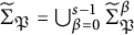 $\widetilde {\Sigma }_{\mathfrak {P}}=\bigcup _{\beta =0}^{s-1}\widetilde {\Sigma }_{\mathfrak {P}}^\beta $
. It follows from [Reference Shirane35, Lemma 4.8] that
 $\widetilde {\Sigma }_{\mathfrak {P}}^\beta $
is connected. For
 $0\leq \beta <\beta '<s$
, if
 $\beta \ne s-\beta '$
, then
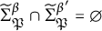 $\widetilde {\Sigma }_{\mathfrak {P}}^\beta \cap \widetilde {\Sigma }_{\mathfrak {P}}^{\beta '}=\emptyset $
by [Reference Shirane35, Theorem 4.3 and Lemma 4.5]. Furthermore, we infer from [Reference Shirane35, Theorem 4.3] and its proof that
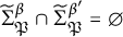 $\widetilde {\Sigma }_{\mathfrak {P}}^\beta \cap \widetilde {\Sigma }_{\mathfrak {P}}^{\beta '}=\emptyset $
for
 $0\leq \beta <\beta '<s$
if
 $\mathfrak {p}_i\ne \mathfrak {p}_j$
for any
 $i\ne j$
; and
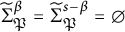 $\widetilde {\Sigma }_{\mathfrak {P}}^\beta =\widetilde {\Sigma }_{\mathfrak {P}}^{s-\beta }=\emptyset $
for
 $0\leq \beta \leq s/2$
otherwise. By using G-combinatorics, we can prove the following theorem.
Theorem 6.4 Let
 $0\leq \beta _1<\beta _2<s$
, and let
 $\mathcal C_i:={ D_i}+\mathcal {L}_i$
be a member of
 $\widetilde {\Sigma }_{\mathfrak {P}}^{\beta _i}$
for
 $i=1,2$
. Then
 $(\mathcal C_1,\mathcal C_2)$
is a Zariski pair if and only if
 $\beta _1\ne s-\beta _2$
.
Proof By [Reference Shirane35, Theorem 4.3(iii)], if
 $\beta _1= s-\beta _2$
, then
 $\mathcal C_1$
and
 $\mathcal C_2$
have the same embedded topology. Suppose that
 $\beta _1\ne s-\beta _2$
. Let
 $\sigma _i\colon Y_i\to {\mathbb {P}}^2$
be the minimal good embedded resolution of
 $\mathcal C_i$
. Note that if the strict transform of
 $\mathcal {L}_i$
is contracted, then we obtain the minimal good embedded resolution of the Artal arrangement
 $\mathcal {A}_i$
given by the quadratic transformation of
 $\mathcal C_i$
. Let
 $\theta _i\colon \pi _1({\mathbb {P}}^2\setminus \mathcal C_i)\to \mathbb Z/d\mathbb Z$
be the surjection given by the composition
 $$\begin{align*}\pi_1({\mathbb{P}}^2\setminus\mathcal C_i)\overset{q_1}{\longrightarrow} \pi_1({\mathbb{P}}^2\setminus { D_i})\overset{q_2}{\longrightarrow} H_1({\mathbb{P}}^2\setminus { D_i};\mathbb Z)\cong\mathbb Z/2d\mathbb Z\overset{q_3}{\longrightarrow}\mathbb Z/d\mathbb Z, \end{align*}$$
where
 $q_1$
is induced the inclusion
 ${\mathbb {P}}^2\setminus \mathcal C_i\to {\mathbb {P}}^2\setminus { D_i}$
,
 $q_2$
is the quotient map by the commutator subgroup, and
 $q_3$
is the natural surjection. Let
 $\phi _i\colon X_i\to {\mathbb {P}}^2$
be the cyclic cover given by
 $\theta _i$
, which is branched along
 $ D_i$
. If there is an equivalence map
 $\varphi _G^\theta \colon \mathrm {Cmb}_G(\mathcal C_1,\theta _1)\to \mathrm { Cmb}(\mathcal C_2,\theta _2)$
, then
 $\varphi _G^\theta $
induces an equivalence map
 $\bar {\varphi }_G^\theta \colon \mathrm { Cmb}_G(\mathcal {A}_1,\theta _1)\to \mathrm {Cmb}_G(\mathcal {A}_2,\theta _2)$
, which is a contradiction to [Reference Shirane35, Theorem 4.3]. Therefore,
 $ \mathrm {Cmb}_G(\mathcal C_i,\theta _i)$
are not G-equivalent, and there is no homeomorphism
 $h\colon {\mathbb {P}}^2\to {\mathbb {P}}^2$
such that
 $ h(D_1)=D_2$
and
 $h(\mathcal {L}_1)=\mathcal {L}_2$
by Theorem 4.4 since
 $\theta _i$
satisfies
 $\theta _i({ \mathfrak {m}_{D_i}})=\pm 1$
for a meridian
 $ \mathfrak {m}_{D_i}$
of
 $ D_i$
. This implies that
 $(\mathcal C_1,\mathcal C_2)$
is a Zariski pair since
 $\deg { D_i}=2d>2$
and
 $ D_i$
is irreducible.
Remark 6.5 For
 $\mathcal C_i$
and
 $\phi _i$
in the proof above, the splitting graphs of
 $\mathcal C_i$
for
 $\phi _i$
are G-equivalent since
 $\phi _i^{-1}(\mathcal {L}_i\setminus { D_i})$
are disjoint union of
 $3d$
components. Namely, it is impossible to prove the difference of their embedded topology by the splitting graphs of
 $\mathcal {L}_i$
for
 $\phi _i$
.
Corollary 6.6 There is a Zariski
 $(\lfloor s/2\rfloor +1)$
-tuple
 $(\mathcal C_0,\dots ,\mathcal C_{\lfloor s/2\rfloor })$
of quasi-triangular curves
 $\mathcal C_i$
of type
 $\mathfrak {P}$
.
Proof Since
 $\widetilde {\Sigma }_{\mathfrak {P}}^\beta \ne \emptyset $
for each
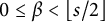 $0\leq \beta <\lfloor s/2\rfloor $
by [Reference Shirane35, Lemma 4.5], the assertion follows from Theorem 6.4.
A
$S^1$
-bundles over
$2$
-manifolds


In this appendix, we recall results on
 $S^1$
-bundles over
 $2$
-manifolds proved in [Reference Waldhausen38]. According to Waldhausen [Reference Waldhausen38], a system of manifolds means a pairwise disjoint finite union of manifolds.
Lemma A.1 [Reference Waldhausen38, Theorem 2.8]
Let
 $p\colon M\to B$
be an
 $S^1$
-bundle over a
 $2$
-manifold B such that B is neither the
 $2$
-sphere
 $S^2$
nor the real projective plane
 ${\mathbb {P}}^2_{\mathbb {R}}$
. Let F be a system of incompressible orientable
 $2$
-manifolds in M such that no component of F with boundary is boundary-parallel. Then there is an isotopy
 $\mathfrak {h}_u\colon M\to M (0\leq u\leq 1)$
such that
 $\mathfrak {h}_0=\mathop {\mathrm {id}}_M$
and
 $\mathfrak {h}_1$
satisfies either
-
(i)
$\mathfrak {h}_1(F)\subset M$
is vertical for p, that is,
$\mathfrak {h}_1(F)=p^{-1}(\ell )$
for some
$\ell \subset B$
. In particular, F is an annulus or a torus; or -
(ii) the restriction of p to
$\mathfrak {h}_1(F)$
is a finite covering.




Remark A.2 With the same assumption of Lemma A.1, if
 $F\cap \partial M$
is vertical, then there is an isotopy
 $\mathfrak {h}_u\colon M\to M$
(
 $0\leq u\leq 1$
) such that
 $\mathfrak {h}_0=\mathop {\mathrm {id}}_M$
,
 $\mathfrak {h}_1(F)\subset M$
is vertical for p, and
 $\mathfrak {h}_u|_{\partial M}=\mathop {\mathrm {id}}_{\partial M}$
for
 $u\in I$
, that is, the isotopy
 $\mathfrak {h}_u$
is constant on the boundary
 $\partial M$
.
By tracing the proof of [Reference Waldhausen38, Theorem 2.8], we can check the above statement. Indeed, the sketch of the proof of [Reference Waldhausen38, Theorem 2.8] with the above assumption is as follows (see [Reference Waldhausen38] for details): Take a system C of vertical annuli such that
 $M\setminus U(C)^\circ $
is an
 $S^1$
-bundle over a disc for a small vertical regular neighborhood
 $U(C)$
of
 $C\subset M$
. We deform M by an isotopy of M constant on
 $\partial M$
so that the number of circles in
 $F\cap C$
is minimal. There is no
 $1$
-manifold with boundary in
 $F\cap C$
since
 $F\cap \partial M$
is vertical. Furthermore, it is proved in [Reference Waldhausen38] that there is no
 $1$
-manifold in
 $F\cap C$
which bounds a disc on F or C. Hence,
 $F\cap C$
consists of only closed
 $1$
-manifolds which are parallel to the boundary of C. There is a deformation of M constant on
 $\partial M$
after which
 $F\cap C$
consists of vertical circles. Let
 $M'$
be the
 $3$
-manifold obtained from M by cutting out along C, that is,
 $M'=M\setminus U(C)^\circ $
. Put
 $F':=F\cap M'$
. Then
 $M'$
is a solid torus, and
 $F'$
consists of boundary-parallel annuli by [Reference Waldhausen38, Theorem 1.9 and Lemma 2.3]. The assertion follows from [Reference Waldhausen38, Lemma 2.4].
Lemma A.3 [Reference Waldhausen38, Lemma 5.1]
Put
 $A:=I\times S^1$
, the annulus. Let
 $p_i\colon A\to I (i=1,2)$
be two
 $S^1$
-bundle projections such that
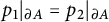 $p_1|_{\partial A}=p_2|_{\partial A}$
. Then there is an isotopy
 $\mathfrak {h}_u\colon A\to A (0\leq u\leq 1)$
such that
 $\mathfrak {h}_0=\mathop {\mathrm {id}}_A$
,
 $p_1=p_2\circ \mathfrak {h}_1$
and
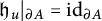 $\mathfrak {h}_u|_{\partial A}=\mathop {\mathrm {id}}_{\partial A}$
for any
 $u\in I$
.
Lemma A.4 [Reference Waldhausen38, Lemma 5.2]
Let T be a torus, and let
 $p_i\colon T\to S^1 (i=1,2)$
be two
 $S^1$
-bundles. If a fiber
 $F_1$
of
 $p_1$
is homotopic to a fiber
 $F_2$
of
 $p_2$
, then there is an isotopy
 $\mathfrak {h}_u\colon T\to T (0\leq u\leq 1)$
such that
 $\mathfrak {h}_0=\mathop {\mathrm {id}}_T$
and
 $p_1=p_2\circ \mathfrak {h}_1$
.
Lemma A.5 [Reference Waldhausen38, Lemma 5.3]
Put
 $V:={\mathbb {D}^2}\times S^1$
, the solid torus. Let
 $p_i\colon V\to { \mathbb {D}^2} (i=1,2)$
be two
 $S^1$
-bundles. If
 $p_1|_{\partial V}=p_2|_{\partial V}$
, then there is an isotopy
 $\mathfrak {h}_u\colon V\to V (0\leq u\leq 1)$
such that
 $\mathfrak {h}_0=\mathop {\mathrm {id}}_V$
,
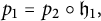 $p_1=p_2\circ \mathfrak {h}_1,$
and
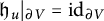 $\mathfrak {h}_u|_{\partial V}=\mathop {\mathrm { id}}_{\partial V}$
.
Theorem A.6 [Reference Waldhausen38, Theorem 5.5]
Let
 $p_i\colon M_i\to B_i (i=1,2)$
be two
 $S^1$
-bundles over
 $2$
-manifolds
 $B_i$
. Assume that
 $B_i$
are not homeomorphic to
 $S^2$
,
 ${\mathbb {P}}^2_{\mathbb {R}}$
,
 $ \mathbb {D}^2$
or
 $I\times S^1\times S^1$
, and that
 $p_i$
has no section if
 $B_i$
is homeomorphic to either the torus or the Klein’s bottle. If
 $h\colon M_1\to M_2$
is a homeomorphism, then there is an isotopy
 $\mathfrak {h}_u\colon M_1\to M_2 (0\leq u\leq 1)$
such that
-
(i)
$\mathfrak {h}_0=h$
, -
(ii) there is a homeomorphism
$h'\colon B_1\to B_2$
such that
$p_2\circ \mathfrak {h}_1=h'\circ p_1$
.



Remark A.7 With the same assumption of Theorem A.6, if
 $\partial M_1\ne \emptyset $
and a homeomorphism
 $h\colon M_1\to M_2$
maps each fiber in
 $\partial M_1$
of
 $p_1$
to that of
 $p_2$
, then there is an isotopy
 $\mathfrak {h}_u\colon M_1\to M_2$
satisfying (i) and (ii) in Theorem A.6 and
-
(iii)
$\mathfrak {h}_u|_{\partial M_1}=h|_{\partial M_1}$
.

Indeed, it can be seen by tracing the proof of [Reference Waldhausen38, Theorem 5.5]. The sketch is as follows (see [Reference Waldhausen38] for details): Let
 $C_1\subset M_1$
be a system of vertical annuli for
 $p_1$
such that
 $M_1\setminus U(C_1)^\circ $
for a small vertical regular neighborhood
 $U(C_1)$
of
 $C_1$
in
 $M_1$
. Then no component of
 $C_1$
is compressible or boundary-parallel. By Remark A.2, there is an isotopy
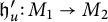 $\mathfrak {h}_u'\colon M_1\to M_2$
(
 $0\leq u\leq 1$
) such that
 $\mathfrak {h}_0'=h$
,
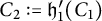 $C_2:=\mathfrak {h}_1'(C_1)$
is vertical for
 $p_2$
and
 $\mathfrak {h}_u'|_{\partial M_1}=h|_{\partial M_1}$
. By Lemma A.3, there is an isotopy
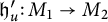 $\mathfrak {h}_u'\colon M_1\to M_2$
(
 $1\leq u\leq 2$
) such that
 $\mathfrak {h}_u'|_{\partial M_1}=h|_{\partial M_1}$
,
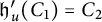 $\mathfrak {h}^{\prime }_u(C_1)=C_2$
for
 $1\leq u\leq 2$
, and
 $\mathfrak {h}^{\prime }_2$
maps each fiber in
 $C_1$
of
 $p_1$
to that in
 $C_2$
of
 $p_2$
. By applying Lemma A.5 to the restriction of
 $\mathfrak {h}^{\prime }_2$
to
 $M_1\setminus U(C_1)^\circ $
, we have an isotopy
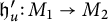 $\mathfrak {h}_u'\colon M_1\to M_2$
(
 $2\leq u\leq 3$
) such that
 $\mathfrak {h}_u'|_{\partial M_1}=h_{\partial M_1}$
for
 $2\leq u\leq 3$
, and
 $\mathfrak {h}^{\prime }_3$
maps every fiber of
 $p_1$
to that of
 $p_2$
. Let
 $\mathfrak {h}_u:=\mathfrak {h}'_{3u}$
(
 $0\leq u\leq 1$
), and let
 $h'\colon B_1\to B_2$
be the homeomorphism induced by
 $\mathfrak{h}_1$
. The isotopy
 $\mathfrak {h}_u$
and the homeomorphism
 $h'\colon B_1\to B_2$
satisfy the assertion.
By the same argument of Remark A.7, we obtain the following lemma.
Lemma A.8 Put
 $M:=I\times S^1\times S^1$
and
 $A:=I\times S^1$
. Let
 $p_i\colon M\to A (i=1,2)$
be two
 $S^1$
-bundles. If a homeomorphism
 $h\colon M\to M$
maps each fiber in
 $\partial M$
of
 $p_1$
to that of
 $p_2$
, then there is an isotopy
 $\mathfrak {h}_u\colon M\to M (0\leq u\leq 1)$
such that
 $\mathfrak {h}_0=h$
,
 $\mathfrak {h}_u|_{\partial M}=h|_{\partial M}$
for
 $0\leq u\leq 1$
, and
 $\mathfrak {h}_1$
maps every fiber of
 $p_1$
to that of
 $p_2$
.
Any
 $S^1$
-bundle
 $p\colon M\to B$
over a
 $2$
-manifold B determines uniquely a disc bundle
 $\overline {p}\colon \overline {M}\to { B}$
up to isotopy such that
 $\partial \overline {M}=M$
and
 $p=\overline {p}|_{M}$
(cf. [Reference Hirzebruch, Neumann and Koh22]).
Let
 $p_i\colon M_i\to B_i$
(
 $i=1,2$
) be two
 $S^1$
-bundles, and let
 $\overline {p}_i\colon \overline {M}_i\to B_i$
be the induced disc bundles. Let
 $\partial B_{i,1},\dots ,\partial B_{i,d_i}$
be the boundary components of
 $B_i$
, and put
 $\overline {\partial M}_{i,j}:=\overline {p}_i^{-1}(\partial B_{i,j})$
. Let
 $$\begin{align*}\overline{\tau}_{i, j}\colon S^1\times { \mathbb{D}^2}\longrightarrow \overline{\partial M}_{i, j}\end{align*}$$
be the trivialization of
 $\overline {\partial M}_{i, j}\subset \overline {M}_i$
with
 $\overline {p}_i\circ \overline {\tau }_{i,j}(t_1,t_2)=t_1$
for each
 $i=1,2$
. We say the following operation to plumb
 $\overline {M}_1$
and
 $\overline {M}_2$
at
 $\overline {\partial M}_{1,j_1}$
and
 $\overline {\partial M}_{2,j_2}$
.
We take the disjoint union
 $\overline {M}_1\sqcup ({ \mathbb {D}^2\times \mathbb {D}^2})\sqcup \overline {M}_2$
and identify by the homeomorphism
 $$ \begin{align*} &\overline{\partial M}_{1,j_1}\ni \overline{\tau}_{1,j_1}(t_1,t_2) \longmapsto (t_1,t_2)\in { (\partial \mathbb{D}^2)\times \mathbb{D}^2}, \\ &\overline{\partial M}_{2,j_2}\ni \overline{\tau}_{2,j_2}(t_1,t_2)\longmapsto (t_2,t_1)\in { \mathbb{D}^2\times (\partial \mathbb{D}^2)} \end{align*} $$
for each
 $(t_1,t_2)\in S^1\times {\mathbb {D}^2}$
. Then we obtain an orientable manifold with boundary, and this manifold is differentiable except along
 $S^1\times S^1\subset { \mathbb {D}^2\times \mathbb {D}^2}$
, where it has a “corner.” By Milnor [Reference Milnor26], this corner can be smoothed, and the smoothing is essentially unique (cf. [Reference Hirzebruch, Neumann and Koh22]). Note that
 $M_i=\partial \overline {M}_i$
(
 $i=1,2$
) are glued by
 $$\begin{align*}J:=\begin{pmatrix} 0&1\\1&0\end{pmatrix}\colon\partial (\overline{\partial M}_{1,j_1})\cong S^1\times S^1\longrightarrow S^1\times S^1\cong\partial(\overline{\partial M}_{2,j_2})\end{align*}$$
via the trivializations
 $\overline {\tau }_{i,j_i}$
.
B Plumbing graphs
In this appendix, we recall results on plumbing graphs in [Reference Neumann28].
B.1 Plumbing graphs and W-graphs
Let
 $\Gamma _{\mathrm {dpg}}=(\Gamma ,\boldsymbol {g},\boldsymbol {e},\mathrm {sgn}; \overline {\mathcal {A}}, \mathcal {A})$
be a decorated plumbing graph of F-normal form with
 $\mathcal {A}(\Gamma )\ne \emptyset $
. We recall [Reference Neumann28, Theorem 5.1] which shows how to obtain a reduced graph structure of the plumbed manifold
 $\mathscr {P}(\Gamma _{\mathrm {dpg}})$
from the F-normal form
 $\Gamma _{\mathrm {dpg}}$
. We obtain the following theorem from [Reference Neumann28, Theorem 5.1].
Theorem B.1 (cf. [Reference Neumann28, Theorem 5.1])
Let
 $\Gamma _{\mathrm {dpg}}=(\Gamma ,\boldsymbol {g},\boldsymbol {e},\mathrm {sgn};\overline {\mathcal {A}},\mathcal {A})$
be a decorated plumbing graph of F-normal form with
 $\mathcal {A}(\Gamma )\ne \emptyset $
. Let
 $\mathcal {S}$
be a subset of
 $\mathcal {Y}(\Gamma )$
which contains precisely one edge of each maximal chain
 $\mathfrak {c}$
of
 $\Gamma $
such that
 $\mathfrak {c}$
is not incident to a boundary vertex. Then
 $\mathbb T_{\mathcal {S}}:=\bigcup _{y\in \mathcal {S}}T_y$
is a reduced graph structure of
 $\mathscr {P}(\Gamma _{\mathrm {dpg}})$
.
Proof As [Reference Neumann28, Appendix], we regard each vertex v in
 $\mathcal {A}(\Gamma )$
as a vertex with
 $\boldsymbol {g}(v)=0$
,
 $\boldsymbol {e}(v)=0,$
and
 $r_v=1$
and
 $\Gamma _{\mathrm {dpg}}$
as an original plumbing graph. Then each chain
 $\mathfrak {c}$
incident to a boundary vertex can be contract by annulus absorptions (R8) in [Reference Neumann28, Proposition 2.1]. Hence,
 $\mathbb T_{\mathcal {S}}$
is a reduced graph structure of
 $\mathscr {P}(\Gamma _{\mathrm {dpg}})$
by the definition of F-normal form and [Reference Neumann28, Theorem 5.1] except the following case:

If
 $\Gamma _{\mathrm {dpg}}$
is the above decorated plumbing graph, then
 $\mathbb T_{\mathcal {S}}$
consists of two tori, and the graph manifold
 $\mathscr {P}(\Gamma _{\mathrm {dpg}})$
with graph structure
 $\mathbb T_{\mathcal {S}}$
is the graph manifold Q in [Reference Waldhausen38, Section 3], which is reduced.
B.2 Orientation reversal
Here, we recall the results in [Reference Neumann28, Section 7]. For a graph manifold M with orientation, let
 $-M$
denote the graph manifold M with reversed orientation. For a plumbing graph
 $\Gamma _{\mathrm {pg}}$
of normal form, the normal form plumbing graph for
 $-\mathscr {P}(\Gamma _{\mathrm {pg}})$
is described in [Reference Neumann28, Theorem 7.1]. We describe the F-normal form decorated plumbing graph of
 $-\mathscr {P}(\Gamma _{\mathrm {dpg}})$
from an F-normal form decorated plumbing graph
 $\Gamma _{\mathrm {dpg}}$
based on [Reference Neumann28, Theorem 7.1].
Let
 $\Gamma _{\mathrm {dpg}}=(\Gamma ,\boldsymbol {g},\boldsymbol {e};\overline {\mathcal {A}}, \mathcal {A})$
be a decorated plumbing graph of F-normal form with
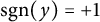 $\mathrm {sgn}(y)=+1$
for each
 $y\in \mathcal {Y}(\Gamma )$
. Let
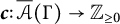 $\boldsymbol {c}\colon \overline {\mathcal {A}}(\Gamma )\to \mathbb Z_{\geq 0}$
be the map such that
 $\boldsymbol {c}(v)$
is the number of maximal chains adjoining v with length
 $>0$
, where chains which both end edges are adjoining v are counted twice, for each
 $v\in \overline {\mathcal {A}}(\Gamma )$
. We abbreviate a sequence of
 $n 2$
’s (
 $n\geq 0$
) as
 $n\cdot 2$
in the following theorem:
 $$\begin{align*}n{\cdot} 2:=\underbrace{2,\dots,2}_n. \end{align*}$$
The following theorem can be proved by the argument of [Reference Neumann28, Theorem 7.1].
Theorem B.2 (cf. [Reference Neumann28, Theorem 7.1])
With the above notation, the F-normal form decorated plumbing graph
 $\Gamma _{\mathrm {dpg}}'=(\Gamma ',\boldsymbol {g}',\boldsymbol {e}',\mathrm {sgn}'; \overline {\mathcal {A}}, \mathcal {A})$
for
 $-\mathscr {P}(\Gamma _{\mathrm {dpg}})$
is obtained from
 $\Gamma _{\mathrm {dpg}}$
as follows:
-
(i)
$\mathcal {A}(\Gamma ')=\mathcal {A}(\Gamma )$
; -
(ii) if
$v\in \overline {\mathcal {A}}(\Gamma )$
which is not on a chain, then
$v\in \overline {\mathcal {A}}(\Gamma ')$
with
$\boldsymbol {g}'(v)=\boldsymbol {g}(v)$
and
$\boldsymbol {e}'(v):=-\boldsymbol {e}(v)-\boldsymbol {c}(v)$
; -
(iii) replace each maximal chain of length
$k\geq 1$
on the left below by the corresponding chain on the right; where the
$c_i$
are determined as follows: if with
$$\begin{align*}(b_1,\dots,b_k)=\left(n_0{\cdot} 2, \ m_1+3, \ n_1{\cdot} 2,\ m_2+3,\dots,\ m_s+3,n_s{\cdot} 2\right) \end{align*}$$
$n_i\geq 0$
and
$m_i\geq 0$
, then
$$\begin{align*}(c_1,\dots, c_\ell)=\left\{\begin{array}{@{}ll} (n_0+1) & (s=0), \\[0.3em] ( n_0+2, \ m_1{\cdot} 2, \ n_1+3,\dots, \ m_s{\cdot} 2,\ n_s+2) & (s>0); \end{array} \right. \end{align*}$$
-
(iv) if
$y\in \mathcal {Y}(\Gamma )$
forms a maximal chain of length
$0$
, then
$y\in \mathcal {Y}(\Gamma ')$
with the same
$o(y),t(y)\in \mathcal {V}(\Gamma ')$
and
$\mathrm {sgn}'(y)=-1$
; -
(v) via the obvious identification
$H_1(\Gamma ^\ast ,\mathcal {A}(\Gamma ))=H_1((\Gamma ')^\ast ,\mathcal {A}(\Gamma '))$
, the homomorphism
$\varepsilon _{\Gamma _{\mathrm {dpg}}'}\colon H_1((\Gamma ')^\ast ,\mathcal {A}(\Gamma '))\to \mathbb Z/2\mathbb Z$
assigns to each relative cycle C of
$((\Gamma ')^\ast ,\mathcal {A}(\Gamma '))$
the number modulo
$2$
of maximal chains on this cycle.








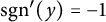




In particular, for
 $b_i,c_j$
in (iii),
 $(b_1,\dots ,b_k)=(c_1,\dots ,c_k)$
if and only if
 $k=1$
and
 $b_1=c_1=2$
.
B.3 Seifert manifolds
For an orientable
 $3$
-manifold M, a Seifert fibration is a partition of M into circles
 $S^1$
, called fibers, such that each fiber in the interior
 $M^\circ $
has closed neighborhood V which is a union of fibers and homeomorphic to a solid torus. A fiber F of M is said to be singular if F is not homotopic to other fibers in a small closed neighborhood V as above, and is said to be regular otherwise. An orientable
 $3$
-manifold is called a Seifert manifold if it admits a Seifert fibration. We assume that a Seifert manifold has a boundary, and that a trivialization is fixed for each boundary component of a Seifert manifold M. The following W-graph
 $\Gamma _{\mathrm {W}}$

is called a Seifert manifold graph since the above
 $\Gamma _{\mathrm {W}}$
describe the Seifert manifold with Seifert invariants
 $((g,r); -s; (\alpha _1,\beta _1),\dots ,(\alpha _m,\beta _m))$
, which corresponds to
 $(g;(1,-s),(\alpha _1,\beta _1),\dots ,(\alpha _m,\beta _m))$
in [Reference Neumann and Raymond29] if
 $r=0$
(cf. [Reference Neumann28, Corollary 5.7] and [Reference Neumann and Raymond29, Theorem 5.1]). In [Reference Neumann and Raymond29], Neumann and Raymond defined the Euler number
 $\boldsymbol {e}(M)$
of a Seifert manifold M given by the W-graph (B.1) with
 $r=0$
, that is, without boundary, as follows:
 $$\begin{align*}\boldsymbol{e}(M):=s-\sum_{i=1}^m\frac{\beta_i}{\alpha_i}. \end{align*}$$
The Euler number
 $\boldsymbol {e}(M)$
can be naturally extend to a Seifert manifold M with boundary having trivialization. The Euler number of
 $-M$
satisfies the following equation (see [Reference Neumann and Raymond29, p. 165]):
 $$ \begin{align} \boldsymbol{e}(-M)=-\boldsymbol{e}(M). \end{align} $$
By [Reference Neumann28, Corollary 5.7], for a Seifert manifold M with boundary corresponding to the above Seifert manifold graph, there is a star-shaped decorated plumbing graph
 $\Gamma _{\mathrm {dpg}}$
of F-normal form, which is in the following form such that
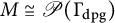 $M\cong \mathscr {P}(\Gamma _{\mathrm {dpg}})$
:

with r boundary vertices, where
 $e=s-m$
,
 $e_{i,j}\leq -2$
for each
 $i,j$
such that
 $$\begin{align*}\frac{\alpha_i}{\alpha_i-\beta_i}=[-e_{i,1},\dots,-e_{i,s_i}] \quad \text{for each } i=1,\dots,m. \end{align*}$$
Then we have
 $$\begin{align*}\boldsymbol{e}(M)=e-\sum_{i=1}^m \frac{1}{[-e_{i,1},\dots,-e_{i,s_i}]}. \end{align*}$$
We can prove the following theorems by the same argument in the case without boundary.
Theorem B.3 (cf. [Reference Neumann and Raymond29, Theorem 1.1])
Let
 $M_1$
and
 $M_2$
be two Seifert manifolds. If there is an orientation preserving homeomorphism
 $h\colon M_1\to M_2$
which preserves fibers, then
 $\boldsymbol {e}(M_1)=\boldsymbol {e}(M_2)$
.
Theorem B.4 (cf. [Reference Neumann and Raymond29, Theorem 5.2])
Let
 $\Gamma _{\mathrm {dpg}}$
be a star-shaped decorated plumbing graph, and let M be a Seifert manifold corresponding to
 $\Gamma _{\mathrm {dpg}}$
. If the intersection form of
 $\Gamma _{\mathrm {dpg}}$
is positive definite (resp. negative definite), then
 $\boldsymbol {e}(M)>0$
(resp.
 $\boldsymbol {e}(M)<0$
).
Acknowledgements
The author thanks Professor E. Artal Bartolo for his valuable comments. He also thanks the reviewers for their valuable comments and suggestions that helped improve this note.



