1. Introduction

A likely consequence of global warming is increased melting from the Greenland ice sheet, resulting in a larger fresh-water flux into the surrounding ocean, a shrinking ice volume and a positive contribution to sea-level change (Reference Church and HoughtonChurch and others, 2001). Over the past decade, various modelling studies were conducted to quantify these volume changes under specified climate scenarios for the 21st century and beyond. the most comprehensive of these ice-sheet studies included the ice-dynamic response of the ice sheet and/or the ongoing adjustment of the ice sheet to past climate changes, but in general it was found that on a century time-scale the bulk of the response is determined by changes in the surface mass balance (Reference VandeWal and OerlemansVan de Wal and Oerlemans,1997; Reference Huybrechts and Wolde.Huybrechts and De Wolde,1999).

First studies prescribed uniform seasonal and regional warming rates and applied precipitation changes proportional to the temperature change with sensitivities derived from ice cores (Reference Huybrechts, Letréguilly and ReehHuybrechts and others, 1991). Runoff was determined locally with a positive degree-day method. Subsequent work relied on climatic input from a two-dimensional zonal mean energy-balance model with seasonal resolution, but kept the simple precipitation dependency (Reference Huybrechts and Wolde.Huybrechts and De Wolde, 1999) or ignored it altogether (Reference De Wolde, Huybrechts, Oerlemans and van deWalDe Wolde and others, 1997; Reference VandeWal and OerlemansVan de Wal and Oerlemans,1997). In these studies, global sea-level rises of 5–20cm were found by the end of the 21st century for typical Intergovernmental Panel on Climate Change- (IPCC-)based climate scenarios. the most recent assessments have included the role of precipitation changes derived directly from atmospheric–oceanic general circulation models (AOGCMs; Reference BugnionBugnion, 2000; Reference Church and HoughtonChurch and others, 2001; Reference Van de Wal, Wild and Wolde.Van de Wal and others, 2001), suggesting that, in a greenhouse-warming world, precipitation increases over Greenland may be larger than often assumed and even largely compensate for the greater runoff.

Here we build further on these studies, and discuss the response of the Greenland ice sheet obtained from an interactive calculation with a three-dimensional dynamic ice-sheet model coupled with a comprehensive atmosphere–ocean– sea-ice general circulation model. This makes it possible to prescribe the seasonally and spatially dependent evolution of precipitation rate and surface temperature, as well as to study the effects of Greenland fresh-water feedback on the surrounding ocean. the latter is related to ongoing speculations about an adverse cooling effect of increased fresh-water input in the North Atlantic Ocean, which could weaken the ventilation of the deep ocean and reduce northward oceanic heat transport, thereby affecting climate over large areas including (northwestern) Europe (e.g. Reference StommelStommel, 1961; Reference Stocker and WrightStocker and Wright, 1991). the approach followed in this paper is still some way from being a truly fully coupled approach, because surface melting is derived from a parameterized interface in terms of temperature and not directly from the heat fluxes provided by the atmosphere model, and because ice-sheet elevation changes do not feed back on the general circulation, though the latter effect can probably be neglected on a century time-scale. the approach, however, differs from previous work in that the climatic forcing is prescribed as a direct output from the atmospheric model and that the oceanic feedback is dealt with synchronously.

2. The Models

The coupled model consists of the Greenland ice sheet model (GISM), on the one hand, which has components describing ice-sheet flow, the solid Earth response and the surface mass balance, and the climate model (AOGCM), on the other hand, which has an atmospheric component (AGCM) and an oceanic component (coupled large-scale ice–ocean (CLIO)).

The ice-dynamics model used in this study corresponds to the version described in Reference Huybrechts and Wolde.Huybrechts and De Wolde (1999). In this model, a distinction is made between grounded ice flow resulting from internal deformation and grounded ice flow resulting from basal sliding. the softness parameter of ice, which determines the rate of deformation, is a function of both the ice temperature and the age of the ice. for that reason, the three-dimensional velocity and temperature fields are calculated in the coupled mode and there is a rigorous tracking of particle trajectories. the procedure basically involves the simultaneous solution of conservation laws for momentum, mass and heat under appropriate simplifications, supplemented by Glen’s flow law with exponent n = 3 (Reference PatersonPaterson, 1994). the model freely generates the ice-sheet geometry in response to prescribed changes of sea level, surface temperature and mass balance. Grounding-line dynamics and local ice shelves are not incorporated explicitly. Instead, the contemporaneous coastline acts as a natural barrier to grounded ice, beyond which all ice is transformed into calf ice. the horizontal resolution is 20 km and there are 31 layers in the vertical.

The mass-balance model distinguishes between snow accumulation, rainfall and runoff, which components are all parameterized in terms of temperature. the melt-and-runoff model is based on the degree-day method as described in Reference Janssens and HuybrechtsJanssens and Huybrechts (2000), but with slightly higher degree-day factors for snow and ice melt of respectively 3.45 and 9.2 mm ˚C^–1d^–1w.e., and a temperature standard deviation σ of 5˚C. These slightly higher parameter values reflect a somewhat steeper modelled surface topography in the ablation zone as compared to the observations for which the calibration in Reference Janssens and HuybrechtsJanssens and Huybrechts (2000) was performed. the process of meltwater retention considers refreezing and the capillary suction effect of the snowpack (Reference Pfeffer, Meier and IllangasekarePfeffer and others, 1991). the fraction of rain depends on the surface temperature and is treated in the same way as the meltwater.

The bedrock adjustment model consists of a rigid elastic plate (lithosphere) that overlies a viscous asthenosphere having only one characteristic response time (Reference Huybrechts and Wolde.Huybrechts and De Wolde, 1999). This treatment gives results similar to the more sophisticated self-gravitating spherical viscoelastic approach, but is much more efficient in its use (Reference Le Meur and HuybrechtsLe Meur and Huybrechts, 1996).

The atmospheric general circulation model required to force the surface climate is the LMD5.3 AGCM (Reference Harzallah and SadournyHarzallah and Sadourny, 1995) developed at the Laboratoire de Météorologie Dynamique, Paris. This finite-difference model uses 64 points regularly spaced in longitude, 50 points regularly spaced in sine of latitude, and 15 vertical levels. Shortwave radiation is modelled after the scheme of Reference Fouquart and BonnelFouquart and Bonnel (1980). Longwave radiation is computed after the method of Reference MorcretteMorcrette (1990). A new release of Morcrette’s scheme has been introduced which takes into account separately each greenhouse gas. the cloud overlapping is random-maximum.The aerosol impact is modelled as a change in surface albedo under clear-sky conditions (Reference Mitchell, Davis, Ingram and Senior.Mitchell and others, 1995). Convection is represented by the combination of a moist adiabatic adjustment and Reference KuoKuo’s (1965) scheme. Le Treut and Li’s (1991) cloud parameterization treats non-convective condensation. Assuming a statistical distribution of water-mixing ratio inside a gridbox, cloud fraction and cloud water content are diagnosed as the fraction of the grid-box in which saturation is reached. the width of this statistical distribution has been adapted inside the boundary layer to condense the humidity more efficiently. This change has led to a better representation of stratiform clouds. Hydrological exchanges between the soil–vegetation system and the atmosphere are determined by the parameterization SECHIBA (Reference Ducoudré, Laval and PerrierDucoudré and others, 1993).

Finally, the ocean–sea-ice component (CLIO) is a primitive-equation, free-surface model. Its horizontal resolution is 363˚, and there are 20 levels along the vertical. to avoid any singularity at the North Pole, two spherical grids connected in the equatorial Atlantic are used (Reference Deleersnijder, vanYpersele and CampinDeleersnijder and others, 1993). the model includes the turbulent closure scheme from Mellor andYamada (Reference Goosse, Campin, Fichefet and DeleersnijderGoosse and others, 1997). Furthermore, it takes into account the formation of deep and bottom waters by open-ocean convection and by the export of dense waters formed over continental shelves (Reference Campin and GoosseCampin and Goosse, 1999). the sea-ice component incorporates parameterizations of the most relevant thermodynamic and dynamic sea-ice processes. An improved version of Reference SemtnerSemtner’s (1976) three-layer model determines the vertical growth and decay of the ice due to thermodynamic processes. to take into consideration the existence of leads and polynyas, a concentration variable related to the heat budget of the open-water area (Reference Fichefet and Morales Maqueda.Fichefet and Morales Maqueda, 1997) is introduced. for the momentum balance, the ice is considered as a two-dimensional viscous–plastic continuum following Reference HiblerHibler (1979).

3. Model Coupling

The various model components are interactively coupled by mutual transfer of relevant physical fluxes and climatic parameters. This coupling is quasi-synchronous taking into account the large spread of model time-steps, which are maximally 1 year for the slowest model components (the ice sheet and its underlying bedrock). to couple the AGCM with CLIO, the fluxes of heat (radiative, latent and sensible), momentum and fresh water (evaporation minus precipitation, plus runoff along coastal boundaries) are transmitted from the atmosphere to the ocean. the sea surface temperature (SST), and sea-ice characteristics (surface temperature, albedo and concentration) are provided to the atmosphere by the ocean. Particular attention is paid to the conservation of energy and water, and no flux correction is used.

The key parameters needed as input for the GISM are the temperature and the precipitation. for present unperturbed conditions, the surface temperature is parameterized from the latitude and the surface elevation (Reference Huybrechts, Letréguilly and ReehHuybrechts and others, 1991). the precipitation rate is taken from a recent update of the Ohmura–Reeh dataset incorporating new data from oversnow traverses in North Greenland (Reference Jung-RothenhäuslerJung-Rothenhäusler,1998). Climatic changes provided by the atmospheric model are subsequently downscaled in the perturbation mode by superimposing temperature anomalies and precipitation ratios (climate changes vs control) from the coarse AGCM grid onto the respective climatic representations on the much finer ice-sheet model grid. Temperature perturbations are applied monthly, but precipitation ratios are only imposed mean annually, because reliable information on their monthly distribution is missing for the reference climate. This in effect assumes that there is a uniform monthly distribution of precipitation all over the ice sheet. for the interpolation of data from the AGCM grid to the GISM grid, we opted to first transform the GISM points in the AGCM grid and subsequently apply Lagrange interpolations. This procedure is more efficient than the reverse procedure as it avoids problems with search functions, choice of weights and discontinuities that would otherwise be associated with the interpolation of the AGCM points which form a scarce and irregular system in the GISM grid.

To close the hydrological cycle, the ice-sheet model in turn yields the annual fresh-water flux feeding back into the ocean, which flux is equally divided into 12 monthly values. This involves the separation of water fluxes into components of ice-sheet runoff, iceberg calving (set equal to the volume flux across the grounding line and calculated as ice thickness times glacier width and depth-averaged horizontal ice velocity), runoff from the ice-free land (set equal to the yearly precipitation), and basal melting below the ice sheet for the different sectors that border the respective oceanic gridboxes of CLIO. the AGCM does not accommodate changes in the geometry of the Greenland ice sheet (elevation and extent) as these would be hardly detectable on the coarse atmospheric grid on the century time-scale that is the subject of this paper. Note, however, that surface elevation changes still feed back on surface temperature, and thus on run-off, as a direct consequence of the parameterization. It is only the (likely very small) effect of ice-sheet changes on the general circulation, and thus mainly on the precipitation field, that is not considered in the runs discussed in this paper.

The ice-dynamic model is only integrated forward after a net yearly surface mass balance has been established, meaning that the ice-sheet response and the associated fresh-water fluxes are delayed by 1 year with respect to the climatic input. This is, however, not a serious problem considering the long response time-scales of the ice sheet and the ocean.

4. Experimental Design

All results are obtained for a time window stretching from 1970 to 2099, with the year 1970 taken as the reference state. Allowance is made for the inertia of the different sub-components by starting simulations at a time early enough to alleviate the effects of specific start-up conditions. Three experiments were performed with the AOGCM. the first one is a 170 year control simulation (CONT). This experiment started from an equilibrium state of the OGCM obtained under a climatological forcing, and from outputs of a 5 year simulation conducted with the AGCM driven by climatological SSTs and sea-ice extents. the greenhouse-gas and sulphate-aerosol concentrations were prescribed to their 1970 values.

The other two experiments with the AOGCM were climate-change experiments: one with the AOGCM alone (SRESB2) in which Greenland fresh-water fluxes had constant ice-sheet runoff and calving, and another with the AOGCM coupled to the GISM (SRESB2G). This set of simulations allows us to forecast climate change and to estimate the role of changes of the Greenland ice sheet in modifying the climate during the next century. the climate-change simulations used the IPCC’s SRESB2 scenario for greenhouse-gas concentrations and sulphate-aerosol loading (Reference Nakicenovic and SwartNakicenovic and others, 2000). This scenario describes a world in which the emphasis is on local solutions to economic, social and environmental sustainability. It is a world with continuously increasing global population, intermediate levels of economic development and moderate technological changes. the climate-change runs started at year 20 of the control experiment, just after the strong initial climate drift. the aerosol model that provided the sulphate-aerosol loading is described in Reference Penner, Chuang and GrantPenner and others (1998). to allow for interannual variability in CONT and SRESB2, precipitation anomalies computed by the AOGCM were added to the reference fresh-water fluxes provided by the GISM.

Because of the long response time-scales of the Greenland ice sheet (of the order of thousands of years), the GISM has first been run during the last two glacial–interglacial cycles to derive initial conditions for coupling with the AOGCM. the model forcing was derived from the Greenland Icecore Project (GRIP) δ¹⁸O record (Reference DansgaardDansgaard and others, 1993) to prescribe temperature and precipitation changes, and from the SPECMAP stack (Reference Imbrie, Berger, Imbrie, Kukla and SaltzmanImbrie and others 1984) to prescribe sea-level changes, similar to the experiments described in Reference Huybrechts and Wolde.Huybrechts and De Wolde (1999). for a good interpretation of the results, an additional control run was performed with the GISM in the uncoupled mode, with climate conditions fixed at the unperturbed 1970 initial state. This experiment makes it possible to establish the background evolution of the ice sheet in the absence of anthropogenic climate changes.

5. Results

5.1. Climate changes from the AOGCM

Figure 1 displays climate changes for the final two decades of the simulation for the region that encompasses the Greenland ice sheet and the North Atlantic Ocean, and including northwestern Europe. Globally, the AOGCM has a climate response of +2.35˚C of surface temperature (SRESB2G – CONT) and a precipitation increase of 3% (SRESB2G/ CONT) for the period 2080–99. the response in the higher northern latitudes is significantly enhanced, with mean annual warmings in excess of 6–7˚C and precipitation increases locally larger than 50%. Averaged over the Greenland ice sheet, mean annual precipitation intensifies by 30– 40% by the end of the 21st century and mean annual temperature increases by 4–5˚C (Fig. 2a). the latter indicates a polar amplification of temperature that is in the mid-range of values established for other AOGCMs (Reference Church and HoughtonChurch and others, 2001). Incidentally, these climate-change results correspond to an average precipitation sensitivity over the Greenland ice sheet of about 6–7% ˚C^–1, very similar to the sensitivities found in Reference Kapsner, Alley, Shuman, Anandakrishnan and Grootes.Kapsner and others (1995) and Reference Cuffey and ClowCuffey and Clow (1997) for the entire GRIP/Greenland Ice Sheet Project 2 (GISP2) ice-core records using a transfer coefficient of 0.42‰ δ¹⁸O ˚C^–1. These precipitation increases are larger than the 0–5% ˚C^–1 employed in most older work in which precipitation is made a direct function of temperature (e.g. Reference Huybrechts, Letréguilly and ReehHuybrechts and others, 1991; De Wolde and others, 1997).

Fig. 1

Mean annual climate changes over Greenland and its surroundings predicted by the coupled atmosphere–oceanic–ice-sheet model for the last two decades of the simulation (2080–99, SRESB2G) compared to the control run for the same time period (CONT).

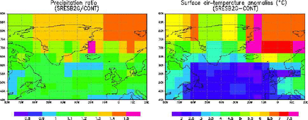
Actual precipitation changes over Greenland scale with the pattern shown in Figure 1 and the present observations, and are therefore largest in the southeastern part of the ice sheet, where present-day precipitation is up to 2ma^–1. Further inspection of the climate-change patterns over Greenland (results not shown) brought to light substantial regional and seasonal differences. Summer temperature rise, which largely controls runoff, is about 2–3˚C by the end of the simulation, whereas winter values peak at 7˚C or more, especially in October and November. These are also features seen in most other AOGCMs, and are related to features such as sea-ice extent. Summer temperature increases are largest in the south and over the central plateau, but close to zero in the northern part. on the regional scale, the patterns of precipitation and temperature change are poorly related, and local and seasonal precipitation sensitivities were found to range anywhere between 0 and 10% ˚C^–1.

5.2. Greenland ice-sheet response

The ice-sheet response during the 21st century shows a clear reduction in area and volume. Total area shrinks by about 1% and total volume varies by an amount equivalent to 4 cm of global sea-level rise (Fig. 2b and c). These changes amount to about half those found in older work for a comparable mean-annual temperature forcing (Reference De Wolde, Huybrechts, Oerlemans and van deWalDe Wolde and others, 1997; Reference Huybrechts and Wolde.Huybrechts and De Wolde, 1999), but are more in line with the 1–4 cm reported in recent studies that use AOGCM results to drive 21st-century mass-balance changes (Reference BugnionBugnion, 2000; Reference Church and HoughtonChurch and others, 2001; Reference Van de Wal, Wild and Wolde.Van de Wal and others, 2001). This is attributed to the smaller temperature rises predicted by AOGCMs in summer, and the larger precipitation increases which partly compensate the increased runoff, an effect which is found to be more important than was assumed in previous studies that derived precipitation change directly from temperature change. We also find that the background evolution (with constant 21st-century climate) is very small compared to the anthropogenically induced response, causing a sea-level change of only 2 mm between 1970 and 2099, or +0.015mma^–1, also in agreement with older studies.

Fig. 2

(a–c) Response of the Greenland ice sheet for the period 1970–2099 driven by climatic output from the AOGCM in the coupled mode. the climatic perturbations shown in (a) are annually and spatially averaged over the entire ice sheet. In (c), 1cm of global sea-level change corresponds to an ice-volume change of 3.98×10¹²m³.

The plots shown in Figure 3 make it possible to distinguish between the static mass-balance effect and the ice-dynamic response. the latter has a component due to both the longer-term background trend, since the ice sheet is still adjusting to past changes in boundary conditions as far back as the last glacial–interglacial transition, and the direct ice-dynamic response to the imposed surface mass-balance changes between 1970 and 2099. the average surface mass-balance changes over the simulation period are displayed in Figure 3a. These are negative in a narrow strip that forms the ablation zone all around the ice sheet, and go up to 1– 2 ma^–1 in the southwestern ablation area where melting is most pronounced. Central areas above the runoff line generally exhibit a slightly larger surface mass balance. Those patterns are typical signatures of climatic warming, giving rise to increased runoff and increased snow accumulation that dominate the response in the lower and higher reaches of the ice sheet, respectively.

Fig. 3

Time-averaged response patterns of Greenland evolution for the period 1970–2099. (a) Static mass-balance response obtained as the mean cumulative mass-balance perturbation with respect to the initial state at 1970; (b) average ice-thickness evolution having a component due to the background trend and the ice-sheet evolution for 1970–2099; (c) ice-dynamic response obtained as the difference between (b) and (a).Values are in ice equivalent. the contour lines are for the presently observed surface elevation and are spaced 500 m apart.

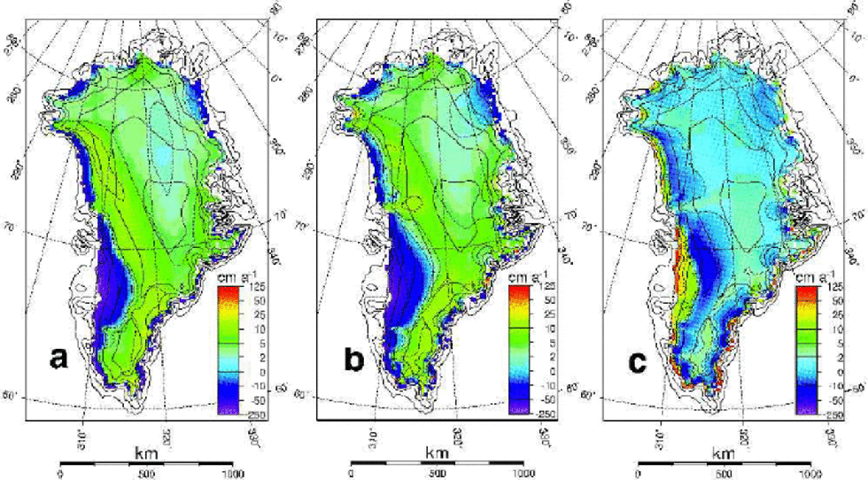
The pattern for the actual ice-thickness changes over the same time period is quite similar to the imposed surface mass-balance change (Fig. 3b), indicating that surface mass-balance variations dominate the response. the difference between Figure 3b and a yields the ice-dynamic response proper (Fig. 3c). Wrapped into this pattern is the longer-term background trend (Reference Huybrechts and Meur.Huybrechts and Le Meur, 1999), of the order of some cm a^–1 at most, but the most conspicuous feature is the thinning of~10 cm a^–1 in the southwest just above the equilibrium line and the thickening of up to 1 ma^–1 further down in the ablation zone. This is a nice demonstration of the ice-dynamic effect described in Reference Huybrechts and Wolde.Huybrechts and De Wolde (1999), and which typically reduces the overall static mass-balance response by 10–20% for simulations spanning the 21st century. the reason is the increased mass-balance gradient in a warmer climate, which is matched by a larger ice flux across the equilibrium line and thus increased transfer of ice mass from the accumulation zone into the melting zone. It leads to a thinning above the equilibrium line, and a dynamic thickening below it. the higher surface level of the ablation zone in turn leads to somewhat less melting than would be the case when ice dynamics were not included, hence the counteracting effect.

5.3. Greenland fresh-water fluxes and climatic impact

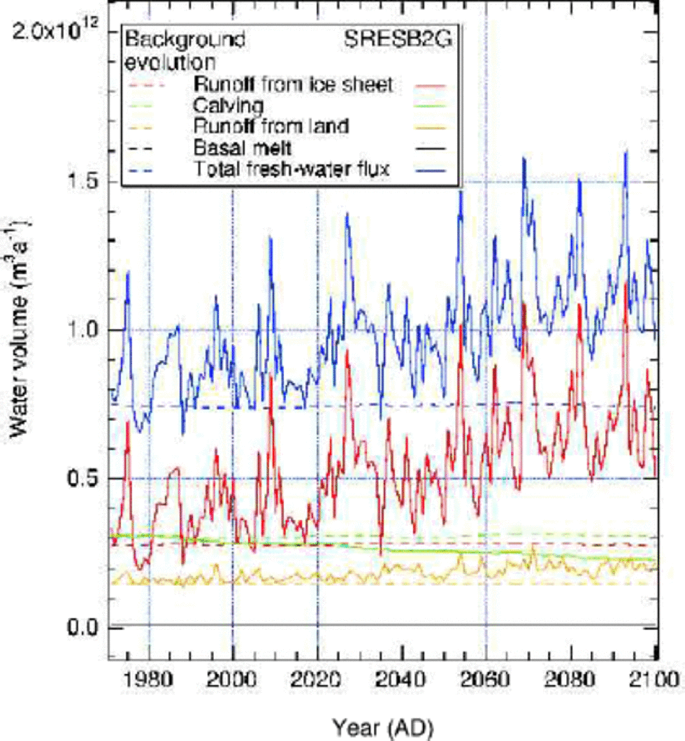
Between 1970 and 2100, the total fresh-water flux increases by >50%, mainly due to the doubled runoff from the ice-sheet surface (Fig. 4). the runoff from land also increases in line with the increased precipitation, but is counterbalanced by a 25% reduction in the ice flux transported across the grounding line (~ calving flux). the latter is due to a thinning of the ice at the margin, so that less ice is able to flow out to the ocean. While the calving flux is, for present-day conditions, twice the runoff from land and about equal to the ice-sheet runoff, after130 years it is about one-third of the ice-sheet run-off and equal to the runoff fromland.The water flux resulting from basal melt is negligible and hardly varies during the simulation. for comparison, the fresh-water components for the unperturbed run are also shown (dashed lines), but these remain almost constant during the simulation.

Fig. 4

Fresh-water flux components from the Greenland continent for the period 1970–2099 shown for the climate change experiment (solid lines) and for the background evolution with zero climatic perturbation (dashed lines). Values are in water equivalent; 1×10¹²m³ is about equal to 0.03 Sv.

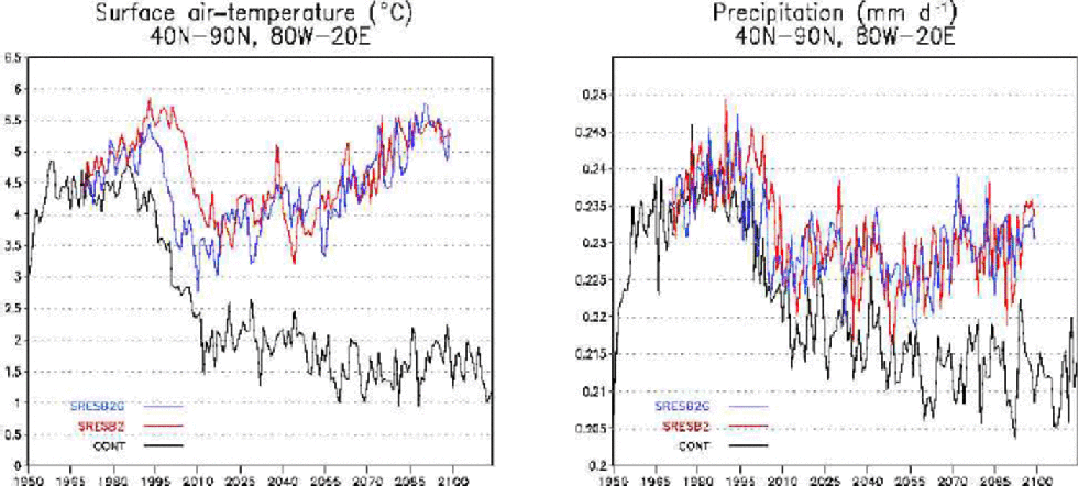
The maximum increase of fresh-water input from the Greenland ice sheet never exceeds 1610¹² m³ a^–1, or about 0.03 Sv. As demonstrated in Figure 5, this meltwater pulse is insufficient to cause significant additional changes in the climate of the North Atlantic region. the evolution of surface air temperature and precipitation rate are not significantly different between an experiment with interactive Greenland fresh-water fluxes (SRESB2G) and a simulation without fresh-water feedback from Greenland (SRESB2). This corroborates simple model studies which indicate that a fresh-water perturbation of at least 0.075 Sv would be required to reach the threshold value to critically weaken the thermohaline circulation in the North Atlantic (Reference RahmstorfRahmstorf, 1995). Such a flux is at least 2.5 times larger than the one obtained in this study, but not unattainable if climatic warming over Greenland were more pronounced than is evident from SRES scenario B2. Furthermore, as the North Atlantic Deep Water formation progressively decreases in the AOGCM’s control simulation, the model sensitivity to an enhanced fresh-water flux is modified. the abrupt decrease in the temperature and precipitation fields simulated over the North Atlantic region (Fig. 5) is a local feature which is not visible on the global average. It is probably linked to modification in the convective zones.

Fig. 5

Spatially and annually averaged changes of surface air temperature and precipitation rate for the rectangle displayed in Figure 1. the blue line is for the coupled experiment driven by IPCC SRES scenario B2 (SRESB2G); the red line refers to a run excluding oceanic feedback from increased Greenland ice-sheet melting (SRESB2).

6. Conclusions

In this paper, we presented results from a coupled ocean– atmosphere–ice-sheet model aimed at investigating the effects of climate warming on the evolution of the Greenland ice sheet and the possible consequences of increased Greenland fresh-water fluxes for the thermohaline circulation of the North Atlantic Ocean. We forced the model with a mid-range IPCC emission scenario (SRESB2) and found an average Greenland temperature rise of about 4.5˚C and an increased precipitation rate of 30–40% by the end of the 21st century. This resulted in a projected Greenland contribution to global sea-level rise of 4 cm between 1970 and 2099. These values are in line with recent projections of Greenland climate and ice-sheet change in which comprehensive AOGCMs are employed, although the implied sea-level change is only about half of those obtained in older work for comparable mean annual temperature changes. That is because of the effect of a larger precipitation rise than previously assumed and because most of the simulated warming occurs in the winter season, when runoff is generally absent. We also presented a series of maps that clearly demonstrated the effect of ice dynamics in modulating the static mass-balance only effect. the implied increase in the fresh-water flux from Greenland is largely due to increased ice-sheet runoff, but is partly counteracted by a reduction of the calving flux as less ice borders the ocean. for the climate scenario under consideration, about 0.03 Sv of additional fresh water enters the North Atlantic. This is found to be insufficient to cross thresholds for weakening of the thermohaline circulation, but threshold magnitudes cited in the literature appear well attainable by the end of the 21st century for not unrealistically larger climatic warmings, and should be investigated in further work.