1 Introduction
Combustion instabilities result from the constructive coupling between acoustic waves and combustion. Because unsteady combustion makes noise and acoustic waves modulate flames, when these phenomena occur with specific phase and sufficient gain, they lead to large pressure oscillations. Fluctuations of the order of the mean chamber pressure are not uncommon, which is at best a nuisance but can lead to the destruction of the combustion device. There are many mechanisms through which combustion instabilities can occur. For example, the parametric instability described by Searby & Rochwerger (Reference Searby and Rochwerger1991) results from the wrinkling of a planar flame in a tube, triggered by the unsteady acceleration of the acoustic field. It was also recently demonstrated that even in anechoic environments, flames may respond to self-generated acoustics, resulting in so-called intrinsic thermo-acoustic instabilities (Hoeijmakers et al. Reference Hoeijmakers, Kornilov, Lopez Arteaga, de Goey and Nijmeijer2014; Courtine, Selle & Poinsot Reference Courtine, Selle and Poinsot2015). However, as proposed by Rogers & Marble (Reference Rogers and Marble1956) and later shown by Poinsot et al. (Reference Poinsot, Trouve, Veynante, Candel and Esposito1987), the vast majority of combustion instabilities stem from the interactions between acoustic eigenmodes of the combustion chamber, coherent vortical structures and flame fronts.
A great deal of progress has been made since the seminal work of Rayleigh (Reference Rayleigh1878), specifically for laminar (Boyer & Quinard Reference Boyer and Quinard1990; Schuller, Durox & Candel Reference Schuller, Durox and Candel2003; Blumenthal et al. Reference Blumenthal, Subramanian, Sujith and Polifke2013) and swirling turbulent flames (Giauque et al. Reference Giauque, Selle, Gicquel, Poinsot, Buechner, Kaufmann and Krebs2005; Candel et al. Reference Candel, Durox, Schuller, Bourgouin and Moeck2014). There is, however, to date no comprehensive theory for the prediction and mitigation of combustion instabilities. The lack of fundamental understanding is particularly striking in the field of liquid rocket engines (LREs). Indeed, the high pressure and temperature at which LREs operate hinder the use of modern visualisation techniques and quantitative laser diagnostics. Moreover, most technologies for the injection of propellants use a multitude of coaxial injectors (typically hundreds) arranged in a compact pattern. For these reasons, despite decades of experimental investigation and the growing need for reliable and affordable access to space, combustion instabilities in rocket engines are still not well understood.
With the advent of high-performance computing, large-eddy simulation (LES) has proven to nicely complement experimental data. Single (Selle et al. Reference Selle, Lartigue, Poinsot, Koch, Schildmacher, Krebs, Prade, Kaufmann and Veynante2004) and multi-burner (Wolf et al. Reference Wolf, Staffelbach, Gicquel, Müller and Poinsot2012) configurations have been computed successfully, shedding light on the physical mechanisms involved in combustion instabilities. Over the past ten years, LES has been applied to coaxial diffusion flames at operating conditions relevant for rocket engines (Tucker et al. Reference Tucker, Menon, Merkle, Oefelein and Yang2008; Huo & Yang Reference Huo and Yang2011; Ruiz et al. Reference Ruiz, Schmitt, Selle, Cuenot and Poinsot2011; Schmitt et al. Reference Schmitt, Méry, Boileau and Candel2011). More recently, the first LES of a full LRE under unstable operating conditions was performed by Urbano et al. (Reference Urbano, Selle, Staffelbach, Cuenot, Schmitt, Ducruix and Candel2016, Reference Urbano, Douasbin, Selle, Staffelbach, Cuenot, Schmitt, Ducruix and Candel2017), giving novel perspectives for the understanding of this type of combustion instability.
The objective of the present study is to take advantage of this unique numerical simulation for a detailed analysis of the driving and damping mechanisms. The configuration and database are first presented in § 2. Then, in § 3, the concept of disturbance energy is presented and applied to the whole combustion chamber. Finally, § 4 focuses on the behaviour of the individual coaxial flames. A methodology that separates the contributions of the two dominant acoustic modes is proposed, shedding light on the coupling mechanisms between acoustics, combustion and hydrodynamics.
2 Configuration and database
The configuration is a 42-injector reduced-scale rocket engine that uses cryogenic hydrogen and oxygen as propellants. The oxidiser to fuel ratio is
 $r=6$
and the mean chamber pressure is
 $p_{c}=80$
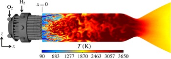
bar. The operating conditions are transcritical in the sense that the chamber pressure is above the critical pressure of both propellants, and the injection temperature of oxygen is below its critical temperature. This engine was designed and operated at DLR Lampoldshausen, and more details are given by Gröning et al. (Reference Gröning, Hardi, Suslov and Oschwald2016) and Urbano et al. (Reference Urbano, Selle, Staffelbach, Cuenot, Schmitt, Ducruix and Candel2016). Figure 1 presents a longitudinal cut of the temperature field in the combustion chamber and the computational domain, which includes the injection manifolds, the 42 coaxial injectors, the combustion chamber and the outlet nozzle.
Overview of the computational domain and of a longitudinal cut of instantaneous temperature field.

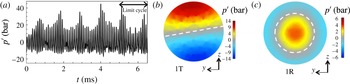
For the considered operating conditions, the engine exhibits a strong combustion instability, which is reproduced in the LES, as shown in figure 2 by the temporal evolution of pressure fluctuations,
 $p^{\prime }$
, at a probe in the chamber. The dominant frequency,
 $f_{1T}=10\,700$
Hz, corresponds to the first transverse mode (1T) of the combustion chamber. The LES of Urbano et al. (Reference Urbano, Selle, Staffelbach, Cuenot, Schmitt, Ducruix and Candel2016) also demonstrated that the second most energetic peak in the experimental spectra corresponds to the first radial mode (1R) of the chamber at
 $f_{1R}=21\,400$
Hz. The spatial structures of these two modes are presented in figure 2, showing the locations of the pressure antinodes and nodal lines. These fields were obtained by performing Fourier transform of 150 3D LES fields, from
 $t=5$
ms to
 $t=6.5$
ms. The LES was performed with the AVBP solver, and details about the models and numerics can be found in Urbano et al. (Reference Urbano, Selle, Staffelbach, Cuenot, Schmitt, Ducruix and Candel2016, Reference Urbano, Douasbin, Selle, Staffelbach, Cuenot, Schmitt, Ducruix and Candel2017).
(a) Temporal evolution of pressure fluctuations at a probe on the chamber wall. (b,c) Transverse cuts showing the spatial structures of the two dominant pressure modes calculated by Fourier transform. Respective frequencies:
 $f_{1T}=10\,700$
Hz and
 $f_{1R}=21\,400$
Hz. The nodal lines are represented by the dashed white lines.

3 Balance of disturbance energy
The present study uses the LES database described in § 2 for the analysis of the disturbance energy,
 $E_{d}$
, which is the extension of the concept of acoustic energy. An exact transport equation for
 $E_{d}$
was initially derived by Myers (Reference Myers1991) and later extended by Brear et al. (Reference Brear, Nicoud, Talei, Giauque and Hawkes2012). Since we address here a transverse mode, the influence of entropy perturbations is neglected. With the additional assumption of chemical equilibrium, which is consistent with the combustion model, and neglecting viscous terms, the balance equation of Brear et al. (Reference Brear, Nicoud, Talei, Giauque and Hawkes2012) reads
 $$\begin{eqnarray}\frac{\unicode[STIX]{x2202}E_{d}}{\unicode[STIX]{x2202}t}+F=R+D.\end{eqnarray}$$
The total disturbance energy,
 $E_{d}$
, in the control volume,
 $V$
, and its flux,
 $F$
, through the boundary,
 $S$
, of this volume are written as
 $$\begin{eqnarray}\displaystyle & \displaystyle E_{d}=\int _{V}(\unicode[STIX]{x1D70C}H^{\prime }-\overline{\boldsymbol{m}}\boldsymbol{\cdot }\boldsymbol{u}^{\prime }-p^{\prime })\,\text{d}V, & \displaystyle\end{eqnarray}$$
 $$\begin{eqnarray}\displaystyle & \displaystyle F=\oint _{S}(\boldsymbol{m}^{\prime }H^{\prime }+\overline{\boldsymbol{m}^{\prime }H^{\prime }})\boldsymbol{\cdot }\boldsymbol{n}\,\text{d}S, & \displaystyle\end{eqnarray}$$
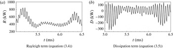
Temporal evolution of
 $R$
and
 $D$
, integrated over the whole combustion chamber.

where
 $\unicode[STIX]{x1D70C}$
is the density,
 $\boldsymbol{u}$
is the velocity,
 $\boldsymbol{m}$
(
 $=\unicode[STIX]{x1D70C}\boldsymbol{u}$
) is the mass flux,
 $\unicode[STIX]{x1D743}=\unicode[STIX]{x1D735}\times \boldsymbol{u}$
is the vorticity,
 $\unicode[STIX]{x1D73B}=\unicode[STIX]{x1D743}\times \boldsymbol{u}$
,
 $H$
is the total enthalpy and
 $\boldsymbol{n}$
is the normalised outward normal to
 $S$
. For all variables, the classical Reynolds decomposition is used:
 $\unicode[STIX]{x1D719}=\overline{\unicode[STIX]{x1D719}}+\unicode[STIX]{x1D719}^{\prime }$
. (Reynolds and time averaged variables are equal under the assumption of ergodicity.) On the right-hand side of (3.1), the Rayleigh term,
 $R$
, represents the contribution of combustion, while
 $D$
accounts for the interaction between acoustics and vortices. They take the forms
 $$\begin{eqnarray}\displaystyle & \displaystyle R=\int _{V}\overline{\left(\frac{\unicode[STIX]{x1D6FC}}{\unicode[STIX]{x1D70C}c_{p}}\right)}(p^{\prime }q^{\prime }+\overline{p^{\prime }q^{\prime }})\,\text{d}V, & \displaystyle\end{eqnarray}$$
 $$\begin{eqnarray}\displaystyle & \displaystyle D=-\int _{V}(\boldsymbol{m}^{\prime }\boldsymbol{\cdot }\unicode[STIX]{x1D73B}^{\prime }+\overline{\boldsymbol{m}^{\prime }\boldsymbol{\cdot }\unicode[STIX]{x1D73B}^{\prime }})\,\text{d}V, & \displaystyle\end{eqnarray}$$
where
 $\unicode[STIX]{x1D6FC}$
is the coefficient of thermal expansion,
 $c_{p}$
is the constant-pressure specific heat capacity,
 $p$
is the pressure and
 $q$
is the heat release rate. It should be noted that the formulation of the Rayleigh term in (3.4) is derived from general thermodynamics and does not assume a specific equation of state. The signs of
 $R$
and
 $D$
are not known a priori. As originally stated by Rayleigh (Reference Rayleigh1878),
 $R>0$
is a necessary condition for a combustion instability to grow. Regarding (3.5),
 $D>0$
corresponds to coherent flow structures producing disturbance energy, which is the mechanism driving jet and cavity noise. Conversely,
 $D<0$
indicates a damping of disturbance energy through vorticity.
Using the database described in § 2 and enclosing the whole combustion chamber in the volume
 $V$
, the temporal evolution of
 $R$
and
 $D$
is plotted in figure 3. The mean Rayleigh term is positive (
 $\overline{R}=470$
kW), which confirms that the flames are indeed the source of the acoustic activity and the engine is exhibiting a combustion instability. Small fluctuations of
 $R$
are visible in figure 3(a); their frequency, which is twice that of the 1T mode, is discussed in § 4.2. Regarding
 $D$
, displayed in figure 3(b), very large fluctuations around zero are observed, indicating that the sign of the transfer of energy between acoustics and vorticity strongly depends on the phase of the eigenmode. At this point, one may speculate that the flow would be perturbed in different ways when the acoustic pressure or acoustic velocity was at its respective peak. This will be confirmed in § 4. The mean value of
 $D$
is negative (
 $\overline{D}=-14$
kW), hence it will be referred to as the dissipation term. The role of
 $D$
in the dissipation of disturbance energy will be further explained in § 4.
4 Analysis of individual flames
The evolution of the source terms in the disturbance-energy balance (3.1), integrated over the whole combustion chamber, only gives a global view of the combustion instability. As expected, it was shown in § 3 that the Rayleigh term,
 $R$
, is driving the instability while the acoustics/vorticity coupling represented by
 $D$
is globally dissipative. It is now interesting to focus on the spatial distribution of source terms and on the individual response of the flames. For this purpose, the combustion chamber is divided into 42 subvolumes, each enclosing a single flame. Boundaries separating individual flames are located at equal distances from neighbouring injectors. Equations (3.4) and (3.5) are now integrated over these individual volumes to draw maps of the contributions of the flames to the total disturbance energy.
4.1 Maps of mean contributions
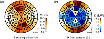
The distribution of the mean Rayleigh term,
 $\overline{R}$
, for individual flames is shown in figure 4(a). Comparing with the spatial structure of the 1T mode (figure 2), which is the dominant mode, it appears that the contribution of the flames located at pressure antinodes is greater than that of the flames close to the nodal line. This is consistent with the fact that the Rayleigh term is proportional to the magnitude of the pressure fluctuations. Moreover,
 $R$
is positive everywhere, meaning that all 42 flames are driving the instability. Regarding the mean acoustics/vorticity interaction term,
 $\overline{D}$
, drawn in figure 4(b), one can see that while the outer flames, located at a pressure antinode of the 1T mode, have a positive contribution, the two inner injector rings provide significant dissipation, i.e.
 $D<0$
.
Maps of mean Rayleigh and dissipation terms, averaged over volumes isolating individual flames. Time averaged over the limit cycle (
 $5\leqslant t\leqslant 6.5$
ms).

4.2 Spectral analysis
The additional information yielded by the spatial distribution of
 $\overline{R}$
and
 $\overline{D}$
in figure 4 is now complemented by a spectral analysis. The objective is to isolate the contributions of the two dominant eigenmodes: the 1T and 1R depicted in figure 2. This analysis is conducted here by performing Fourier transforms (FTs) on the time-resolved database of 3D LES fields. Similar results (not shown here) have been obtained via the dynamic mode decomposition methodology of Schmid (Reference Schmid2010), which may be more efficient for samples with fewer limit-cycle oscillations. Because (3.4) and (3.5) are nonlinear functions of the flow variables, their spectral analysis is not straightforward. It is, however, investigated whether the spectral analysis of
 $R$
and
 $D$
could be useful. The present analysis neglects nonlinear interactions between modes, which is a limitation, especially given the large amplitudes encountered in combustion instabilities. The results are therefore not quantitative but still allow qualitative interpretation.
4.2.1 Contributions of the flames
The Rayleigh term is analysed first. The pressure and heat release rate spectral decompositions are written as
 $$\begin{eqnarray}\left.\begin{array}{@{}c@{}}p^{\prime }(\boldsymbol{x},t)=\tilde{p}(\boldsymbol{x})\cos (\unicode[STIX]{x1D714}t-\unicode[STIX]{x1D719}^{p}(\boldsymbol{x})),\\ q^{\prime }(\boldsymbol{x},t)=\tilde{q}(\boldsymbol{x})\cos (\unicode[STIX]{x1D714}t-\unicode[STIX]{x1D719}^{q}(\boldsymbol{x})),\end{array}\right\}\end{eqnarray}$$
where
 $\boldsymbol{x}$
is the spatial coordinate,
 $t$
is the time,
 $\tilde{p}$
and
 $\unicode[STIX]{x1D719}^{p}$
(respectively
 $\tilde{q}$
and
 $\unicode[STIX]{x1D719}^{q}$
) are the modulus and phase of the pressure (respectively heat release rate) mode. Combination with (3.4) yields
 $$\begin{eqnarray}R=\int _{V}\left[\overline{\left(\frac{\unicode[STIX]{x1D6FC}}{\unicode[STIX]{x1D70C}C_{p}}\right)}\tilde{p}\tilde{q}\left(\frac{1}{2}\cos (2\unicode[STIX]{x1D714}t-(\unicode[STIX]{x1D719}^{p}+\unicode[STIX]{x1D719}^{q}))+\cos (\unicode[STIX]{x1D719}^{p}-\unicode[STIX]{x1D719}^{q})\right)\right]\text{d}V.\end{eqnarray}$$
The first observation is that for a mode with pulsation
 $\unicode[STIX]{x1D714}$
, the associated Rayleigh contribution oscillates at
 $2\unicode[STIX]{x1D714}$
. This explains the fluctuations in figure 3(a) at twice the frequency of the 1T mode. Consequently, in the FT of
 $R$
, the contribution of the 1T mode corresponds to the peak at
 $2f_{1T}$
. Its magnitude, denoted
 $\widetilde{R}$
, is obtained from (4.2),
 $$\begin{eqnarray}\widetilde{R}=\frac{1}{2}\int _{V}\overline{\left(\frac{\unicode[STIX]{x1D6FC}}{\unicode[STIX]{x1D70C}C_{p}}\right)}\tilde{p}\tilde{q}\,\text{d}V.\end{eqnarray}$$
On the other hand, taking the average of (4.2) yields
 $$\begin{eqnarray}\overline{R}=\int _{V}\overline{\left(\frac{\unicode[STIX]{x1D6FC}}{\unicode[STIX]{x1D70C}C_{p}}\right)}\tilde{p}\tilde{q}\cos (\unicode[STIX]{x1D719}^{p}-\unicode[STIX]{x1D719}^{q})\,\text{d}V.\end{eqnarray}$$
Consequently, the mean Rayleigh source term
 $\overline{R}$
in a given control volume is related to the peak in the FT of
 $R$
at twice the frequency of the considered mode through
 $$\begin{eqnarray}\overline{R}=2\widetilde{R}\cos (\unicode[STIX]{x1D719}^{p}-\unicode[STIX]{x1D719}^{q}).\end{eqnarray}$$
Equation (4.5) therefore establishes that under the assumption of linear interaction, the FT of
 $R$
is qualitatively indicative of the contribution of the modes to the disturbance-energy budget. (Equation (4.5) is strictly valid only when the phase difference
 $(\unicode[STIX]{x1D719}^{p}-\unicode[STIX]{x1D719}^{q})$
is constant in
 $V$
.)
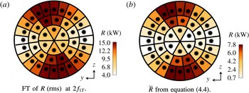
The comparison between
 $\overline{R}$
and the FT of
 $R$
is presented in figure 5 for the 1T mode. They are qualitatively very similar, despite being quantitatively different. The agreement is favoured by the fact that
 $R$
is positive everywhere under these conditions. Caution would be needed in the case of sign change, as shown in § 4.2.2. Figure 5(b) confirms that the flames located close to the pressure nodal line have a marginal contribution to the disturbance-energy budget. The flames driving the combustion instability are those located at a pressure antinode.
Comparison of Rayleigh maps for the 1T mode, obtained using the FT of
 $R$
and the reconstruction of
 $\overline{R}$
using the FT of pressure and heat release rate fluctuations.

4.2.2 Interaction between acoustics and vorticity
The same methodology is applied to (3.5), which was shown in § 3 to be the main source of dissipation of disturbance energy. Taking advantage of the fact that
 $\boldsymbol{m}\boldsymbol{\cdot }\unicode[STIX]{x1D73B}=0$
, equation (3.5) is recast as (cf. appendix A)
 $$\begin{eqnarray}D=\int _{V}(\boldsymbol{m}^{\prime }\boldsymbol{\cdot }\overline{\unicode[STIX]{x1D73B}}+\overline{\boldsymbol{m}}\boldsymbol{\cdot }\unicode[STIX]{x1D73B}^{\prime }+2\overline{\unicode[STIX]{x1D73B}}\boldsymbol{\cdot }\overline{\boldsymbol{m}})\,\text{d}V.\end{eqnarray}$$
Using similar notations to those in § 4.2.1, the spectral decompositions of density, velocity and vorticity fluctuations are
 $$\begin{eqnarray}\left.\begin{array}{@{}c@{}}\unicode[STIX]{x1D70C}^{\prime }(\boldsymbol{x},t)=\tilde{\unicode[STIX]{x1D70C}}(\boldsymbol{x})\cos (\unicode[STIX]{x1D714}t-\unicode[STIX]{x1D719}^{\unicode[STIX]{x1D70C}}(\boldsymbol{x})),\\ u_{i}^{\prime }(\boldsymbol{x},t)=\tilde{u} _{i}(\boldsymbol{x})\cos (\unicode[STIX]{x1D714}t-\unicode[STIX]{x1D719}_{i}^{u}(\boldsymbol{x})),\\ \unicode[STIX]{x1D709}_{i}^{\prime }(\boldsymbol{x},t)=\tilde{\unicode[STIX]{x1D709}}_{i}(\boldsymbol{x})\cos (\unicode[STIX]{x1D714}t-\unicode[STIX]{x1D719}_{i}^{\unicode[STIX]{x1D709}}(\boldsymbol{x})),\end{array}\right\}\end{eqnarray}$$
where the subscript
 $i\in \{1,2,3\}$
indicates the component in the Cartesian frame of reference. Tedious but straightforward algebra shows that (cf. appendix A)
 $$\begin{eqnarray}D=\int _{V}(D_{1}+D_{2})\,\text{d}V,\end{eqnarray}$$
where
 $$\begin{eqnarray}\displaystyle D_{1} & = & \displaystyle \overline{\unicode[STIX]{x1D701}}_{k}[\overline{\unicode[STIX]{x1D70C}}\tilde{u_{k}}\cos (\unicode[STIX]{x1D714}t-\unicode[STIX]{x1D719}_{k}^{u})+\tilde{\unicode[STIX]{x1D70C}}\overline{u_{k}}\cos (\unicode[STIX]{x1D714}t-\unicode[STIX]{x1D719}^{\unicode[STIX]{x1D70C}})]\nonumber\\ \displaystyle & & \displaystyle +\,\overline{m_{k}}[\unicode[STIX]{x1D700}^{ijk}\overline{\unicode[STIX]{x1D709}_{i}}\tilde{u_{j}}\cos (\unicode[STIX]{x1D714}t-\unicode[STIX]{x1D719}_{j}^{u})+\unicode[STIX]{x1D700}^{ijk}\tilde{\unicode[STIX]{x1D709}_{i}}\overline{u_{j}}\cos (\unicode[STIX]{x1D714}t-\unicode[STIX]{x1D719}_{i}^{\unicode[STIX]{x1D709}})]\end{eqnarray}$$
and
 $$\begin{eqnarray}\displaystyle D_{2} & = & \displaystyle \tilde{\unicode[STIX]{x1D70C}}\tilde{u_{k}}\unicode[STIX]{x1D700}^{ijk}\overline{\unicode[STIX]{x1D709}_{i}}\overline{u_{j}}\left[{\textstyle \frac{1}{2}}\cos (2\unicode[STIX]{x1D714}t-(\unicode[STIX]{x1D719}^{\unicode[STIX]{x1D70C}}+\unicode[STIX]{x1D719}_{k}^{u}))+\cos (\unicode[STIX]{x1D719}^{\unicode[STIX]{x1D70C}}-\unicode[STIX]{x1D719}_{k}^{u})\right]\nonumber\\ \displaystyle & & \displaystyle +\,\overline{\unicode[STIX]{x1D70C}}\overline{u_{k}}\unicode[STIX]{x1D700}^{ijk}\tilde{\unicode[STIX]{x1D709}_{i}}\tilde{u_{j}}\left[{\textstyle \frac{1}{2}}\cos (2\unicode[STIX]{x1D714}t-(\unicode[STIX]{x1D719}_{i}^{\unicode[STIX]{x1D709}}+\unicode[STIX]{x1D719}_{j}^{u}))+\cos (\unicode[STIX]{x1D719}_{i}^{\unicode[STIX]{x1D709}}-\unicode[STIX]{x1D719}_{j}^{u})\right]\nonumber\\ \displaystyle & & \displaystyle +\,\tilde{\unicode[STIX]{x1D70C}}\tilde{u_{k}}\unicode[STIX]{x1D700}^{ijk}\tilde{\unicode[STIX]{x1D709}_{i}}\tilde{u_{j}}\left[{\textstyle \frac{1}{4}}\cos (2\unicode[STIX]{x1D714}t-(\unicode[STIX]{x1D719}^{\unicode[STIX]{x1D70C}}+\unicode[STIX]{x1D719}_{k}^{u}))\cos (\unicode[STIX]{x1D719}_{i}^{\unicode[STIX]{x1D709}}-\unicode[STIX]{x1D719}_{j}^{u})\right.\nonumber\\ \displaystyle & & \displaystyle +\left.{\textstyle \frac{1}{4}}\cos (2\unicode[STIX]{x1D714}t-(\unicode[STIX]{x1D719}_{i}^{\unicode[STIX]{x1D709}}+\unicode[STIX]{x1D719}_{j}^{u}))\cos (\unicode[STIX]{x1D719}^{\unicode[STIX]{x1D70C}}-\unicode[STIX]{x1D719}_{k}^{u})+{\textstyle \frac{1}{2}}\cos (\unicode[STIX]{x1D719}^{\unicode[STIX]{x1D70C}}-\unicode[STIX]{x1D719}_{k}^{u})\cos (\unicode[STIX]{x1D719}_{i}^{\unicode[STIX]{x1D709}}-\unicode[STIX]{x1D719}_{j}^{u})\right]\!.\qquad \quad\end{eqnarray}$$
Equations (4.8)–(4.10) indicate that
 $D$
contains two fluctuating components, one at the frequency of the considered acoustic mode and one at twice this frequency. The corresponding average is
 $$\begin{eqnarray}\displaystyle \overline{D} & = & \displaystyle \int _{V}\left(\vphantom{{\textstyle \frac{1}{2}}}\unicode[STIX]{x1D700}^{ijk}\overline{\unicode[STIX]{x1D709}_{i}}\overline{u_{j}}\tilde{\unicode[STIX]{x1D70C}}\tilde{u_{k}}\cos (\unicode[STIX]{x1D719}^{\unicode[STIX]{x1D70C}}-\unicode[STIX]{x1D719}_{k}^{u})+\overline{\unicode[STIX]{x1D70C}}\overline{u_{k}}\unicode[STIX]{x1D700}^{ijk}\tilde{\unicode[STIX]{x1D709}_{i}}\tilde{u_{j}}\cos (\unicode[STIX]{x1D719}_{i}^{\unicode[STIX]{x1D709}}-\unicode[STIX]{x1D719}_{j}^{u})\right.\nonumber\\ \displaystyle & & \displaystyle +\left.{\textstyle \frac{1}{2}}\unicode[STIX]{x1D700}^{ijk}\tilde{\unicode[STIX]{x1D709}_{i}}\tilde{u_{j}}\tilde{\unicode[STIX]{x1D70C}}\tilde{u_{k}}\cos (\unicode[STIX]{x1D719}^{\unicode[STIX]{x1D70C}}-\unicode[STIX]{x1D719}_{k}^{u})\cos (\unicode[STIX]{x1D719}_{i}^{\unicode[STIX]{x1D709}}-\unicode[STIX]{x1D719}_{j}^{u})\right)\text{d}V.\end{eqnarray}$$
Noting that
 $\overline{D_{1}}=0$
, the peak at
 $\unicode[STIX]{x1D714}$
in the FT of
 $D$
is not related to the mean dissipation,
 $\overline{D}$
. Unlike the Rayleigh term, the relation between
 $\overline{D}$
and the second peak in the FT of
 $D$
is not straightforward because of the many phase differences involved.
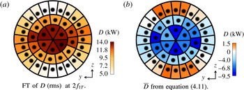
The comparison between the FTs of
 $D$
and
 $\overline{D}$
is presented in figure 6 for the 1T mode. It appears that because
 $\overline{D}$
changes sign, the two quantities are qualitatively different. Figure 6(a) looks like the absolute value of
 $\overline{D}$
, meaning that the FT of
 $D$
is not a very useful diagnostic in this case. However, figure 6(b) provides a better picture than figure 4(b) regarding the dissipation associated with the dominant acoustic mode. It is clear that the flames located around the nodal line provide massive dissipation. Indeed, flames at a pressure node experience strong transverse acoustic velocity, which is known to induce flapping, jet flattening and flame shortening (Baillot et al.
Reference Baillot, Blaisot, Boisdron and Dumouchel2009; Hardi et al.
Reference Hardi, Martinez, Oschwald and Dally2014; Hakim et al.
Reference Hakim, Schmitt, Ducruix and Candel2015). These motions take their energy from the acoustic field, explaining the local dissipation.
Comparison of dissipation maps for the 1T mode, obtained using the FT of
 $D$
and the reconstruction of
 $\overline{D}$
using the FT of velocity and vorticity fluctuations.

4.2.3 Application to the 1R mode
The same methodology is now applied to the 1R mode in order to analyse how the flames contribute to
 $\overline{R}$
and
 $\overline{D}$
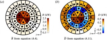
for this mode which has a higher frequency and a different spatial structure (cf. figure 2). The Rayleigh term, displayed in figure 7(a), is positive, indicating that the 1R mode is also unstable. The flames in the inner ring, located at a pressure antinode, provide most of the drive. The outer ring, also at a pressure antinode, has a small contribution, which is speculated to be caused by a phase mismatch between
 $p^{\prime }$
and
 $q^{\prime }$
. The intermediate ring exhibits a small Rayleigh term, which is consistent with the location of the pressure nodal line. The dissipation map for the 1R mode plotted in figure 7(b) confirms the observation that the flames on the pressure nodal line (i.e. the middle injector ring) provide dissipation. The analysis for the 1R mode is therefore consistent with that of the 1T mode.
Maps of Rayleigh and dissipation terms for the 1R mode.

It is interesting to discuss the relative importance of the two source terms in the two dominant unstable modes. For the 1T mode, the global Rayleigh index is
 $\overline{R}_{1T}=160$
kW and the dissipation
 $\overline{D}_{1T}=-110$
kW (these values are obtained by integrating the maps of figures 5
b and 6
b). For the 1R mode,
 $\overline{R}_{1R}=30$
kW and
 $\overline{D}_{1R}=1.2$
kW. Despite its smaller Rayleigh index, the 1R mode reaches an amplitude comparable to that of the 1T mode because of the large dissipation
 $\overline{D}_{1T}$
. This illustrates the necessity to understand and quantify dissipation mechanisms, while most studies of combustion instabilities focus solely on the Rayleigh index.
5 Conclusion
The analysis of disturbance-energy source terms presented in this work gives novel perspectives on the mechanisms at play during transverse combustion instabilities in an LRE. Using a time-resolved database of 3D fields from an LES, a spectral analysis of the individual flame contributions was presented. The two source terms accounting for the interaction between acoustics and unsteady combustion (
 $R$
) and acoustics and hydrodynamics (
 $D$
) were studied. As expected, the well-known Rayleigh index,
 $R$
, drives the instability, with dominant contribution from the flames near a pressure antinode. This indicates that for the determination of the combustion stability, the response of these flames to the bulk pressure fluctuations at the injector outlets seems to be more important than their response to transverse acoustic-velocity fluctuations. A small mean dissipation results from
 $D$
. However, the spectral analysis has shown that flames located at a pressure node provide very large dissipation, affecting the stability of the corresponding eigenmode. The associated mechanism is a transfer of energy from the transverse acoustic-velocity field to the flapping motion of the flame.
Acknowledgements
This investigation was carried out in the framework of the French–German REST program initiated by Airbus Safran Launchers, CNES, DLR and ONERA. Support provided by Airbus Safran Launchers, the prime contractor of the Ariane 5 and Ariane 6 launchers, is gratefully acknowledged. This work was granted access to the high-performance computing resources of IDRIS under the allocation x20162b7036 made by Grand Equipement National de Calcul Intensif. The research leading to these results has received funding from the European Research Council under the European Union’s Seventh Framework Programme (FP/2007-2013)/ERC Grant Agreement ERC-AdG 319067-INTECOCIS.
Appendix A. Derivation of the dissipation term (
 $D$
)

Using the definition of the fluctuating quantities, the first term of equation (3.5) is written as
 $$\begin{eqnarray}\displaystyle -\boldsymbol{m}^{\prime }\boldsymbol{\cdot }\unicode[STIX]{x1D73B}^{\prime } & = & \displaystyle -(\boldsymbol{m}-\overline{\boldsymbol{m}})\boldsymbol{\cdot }(\unicode[STIX]{x1D73B}-\overline{\unicode[STIX]{x1D73B}})\nonumber\\ \displaystyle & = & \displaystyle -\boldsymbol{m}\boldsymbol{\cdot }\unicode[STIX]{x1D73B}+\boldsymbol{m}\boldsymbol{\cdot }\overline{\unicode[STIX]{x1D73B}}+\overline{\boldsymbol{m}}\boldsymbol{\cdot }\unicode[STIX]{x1D73B}-\overline{\boldsymbol{m}}\boldsymbol{\cdot }\overline{\unicode[STIX]{x1D73B}}.\end{eqnarray}$$
Noting that
 $\boldsymbol{m}\boldsymbol{\cdot }\unicode[STIX]{x1D73B}=\unicode[STIX]{x1D70C}\boldsymbol{u}\boldsymbol{\cdot }\unicode[STIX]{x1D743}\times \boldsymbol{u}=0$
, taking the average of (A 1) yields
 $$\begin{eqnarray}-\overline{\boldsymbol{m}^{\prime }\boldsymbol{\cdot }\unicode[STIX]{x1D73B}^{\prime }}=\overline{\boldsymbol{m}}\boldsymbol{\cdot }\overline{\unicode[STIX]{x1D73B}}.\end{eqnarray}$$
Using (A 1) and (A 2), equation (4.6) easily follows from (3.5).
The goal is now to write (4.6) in terms of primitive variables – density, velocity and vorticity. For this purpose, the averages and fluctuations of
 $\boldsymbol{m}$
and
 $\unicode[STIX]{x1D73B}$
are written as
 $$\begin{eqnarray}\displaystyle & \overline{\boldsymbol{m}}=\overline{\unicode[STIX]{x1D70C}}\,\overline{\boldsymbol{u}}+\overline{\unicode[STIX]{x1D70C}^{\prime }\boldsymbol{u}^{\prime }}, & \displaystyle\end{eqnarray}$$
 $$\begin{eqnarray}\displaystyle & \overline{\unicode[STIX]{x1D73B}}=\overline{\unicode[STIX]{x1D743}}\times \overline{\boldsymbol{u}}+\overline{\unicode[STIX]{x1D743}^{\prime }\times \boldsymbol{u}^{\prime }}, & \displaystyle\end{eqnarray}$$
 $$\begin{eqnarray}\displaystyle & \boldsymbol{m}^{\prime }=\overline{\unicode[STIX]{x1D70C}}\boldsymbol{u}^{\prime }+\unicode[STIX]{x1D70C}^{\prime }\overline{\boldsymbol{u}}+\unicode[STIX]{x1D70C}^{\prime }\boldsymbol{u}^{\prime }-\overline{\unicode[STIX]{x1D70C}^{\prime }\boldsymbol{u}^{\prime }}, & \displaystyle\end{eqnarray}$$
 $$\begin{eqnarray}\displaystyle & \unicode[STIX]{x1D73B}^{\prime }=\overline{\unicode[STIX]{x1D743}}\times \boldsymbol{u}^{\prime }+\unicode[STIX]{x1D743}^{\prime }\times \overline{\boldsymbol{u}}+\unicode[STIX]{x1D743}^{\prime }\times \boldsymbol{u}^{\prime }-\overline{\unicode[STIX]{x1D743}^{\prime }\times \boldsymbol{u}^{\prime }}. & \displaystyle\end{eqnarray}$$
Using (A 3)–(A 6), equation (4.6) is rearranged as (4.8), where
 $D_{1}$
and
 $D_{2}$
contain respectively first- and second-order terms in the fluctuating quantities and are given by
 $$\begin{eqnarray}\displaystyle & D_{1}=\overline{\unicode[STIX]{x1D73B}}\boldsymbol{\cdot }(\overline{\unicode[STIX]{x1D70C}}\boldsymbol{u}^{\prime }+\unicode[STIX]{x1D70C}^{\prime }\overline{\boldsymbol{u}})+\overline{\boldsymbol{m}}\boldsymbol{\cdot }(\overline{\unicode[STIX]{x1D743}}\times \boldsymbol{u}^{\prime }+\unicode[STIX]{x1D743}^{\prime }\times \overline{\boldsymbol{u}}), & \displaystyle\end{eqnarray}$$
 $$\begin{eqnarray}\displaystyle & D_{2}=\overline{\unicode[STIX]{x1D70C}}\,\overline{\boldsymbol{u}}\boldsymbol{\cdot }[\unicode[STIX]{x1D743}^{\prime }\times \boldsymbol{u}^{\prime }+\overline{\unicode[STIX]{x1D743}^{\prime }\times \boldsymbol{u}^{\prime }}]+\overline{\unicode[STIX]{x1D743}}\times \overline{\boldsymbol{u}}\boldsymbol{\cdot }[\unicode[STIX]{x1D70C}^{\prime }\boldsymbol{u}^{\prime }+\overline{\unicode[STIX]{x1D70C}^{\prime }\boldsymbol{u}^{\prime }}]+\unicode[STIX]{x1D70C}^{\prime }\boldsymbol{u}^{\prime }\boldsymbol{\cdot }\overline{\unicode[STIX]{x1D743}^{\prime }\times \boldsymbol{u}^{\prime }}+\overline{\unicode[STIX]{x1D70C}^{\prime }\boldsymbol{u}^{\prime }}\boldsymbol{\cdot }\unicode[STIX]{x1D743}^{\prime }\times \boldsymbol{u}^{\prime }. & \displaystyle \nonumber\\ \displaystyle & & \displaystyle\end{eqnarray}$$
The spectral decompositions of density, velocity and vorticity fluctuations given by (4.7) are used to express the fluctuating quantities in
 $D_{1}$
and
 $D_{2}$
and to obtain (4.9) and (4.10). In particular, making use of trigonometric properties, the terms
 $\unicode[STIX]{x1D70C}^{\prime }\boldsymbol{u}^{\prime }$
,
 $\unicode[STIX]{x1D743}^{\prime }\times \boldsymbol{u}^{\prime }$
and their averages have been replaced by
 $$\begin{eqnarray}\displaystyle & \unicode[STIX]{x1D743}^{\prime }\times \boldsymbol{u}^{\prime }={\textstyle \frac{1}{2}}\unicode[STIX]{x1D700}^{ijk}\tilde{\unicode[STIX]{x1D709}_{i}}\tilde{u_{j}}[\cos (2\unicode[STIX]{x1D714}t-(\unicode[STIX]{x1D719}_{i}^{\unicode[STIX]{x1D709}}+\unicode[STIX]{x1D719}_{j}^{u}))+\cos (\unicode[STIX]{x1D719}_{i}^{\unicode[STIX]{x1D709}}-\unicode[STIX]{x1D719}_{j}^{u})], & \displaystyle\end{eqnarray}$$
 $$\begin{eqnarray}\displaystyle & \overline{\unicode[STIX]{x1D743}^{\prime }\times \boldsymbol{u}^{\prime }}={\textstyle \frac{1}{2}}\unicode[STIX]{x1D700}^{ijk}\tilde{\unicode[STIX]{x1D709}_{i}}\tilde{u_{j}}\cos (\unicode[STIX]{x1D719}_{i}^{\unicode[STIX]{x1D709}}-\unicode[STIX]{x1D719}_{j}^{u}), & \displaystyle\end{eqnarray}$$
 $$\begin{eqnarray}\displaystyle & \unicode[STIX]{x1D70C}^{\prime }\boldsymbol{u}^{\prime }={\textstyle \frac{1}{2}}\tilde{\unicode[STIX]{x1D70C}}\tilde{u_{k}}[\cos (2\unicode[STIX]{x1D714}t-(\unicode[STIX]{x1D719}^{\unicode[STIX]{x1D70C}}+\unicode[STIX]{x1D719}_{k}^{u}))+\cos (\unicode[STIX]{x1D719}^{\unicode[STIX]{x1D70C}}-\unicode[STIX]{x1D719}_{k}^{u})], & \displaystyle\end{eqnarray}$$
 $$\begin{eqnarray}\displaystyle & \overline{\unicode[STIX]{x1D70C}^{\prime }\boldsymbol{u}^{\prime }}={\textstyle \frac{1}{2}}\tilde{\unicode[STIX]{x1D70C}}\tilde{u_{k}}\cos (\unicode[STIX]{x1D719}^{\unicode[STIX]{x1D70C}}-\unicode[STIX]{x1D719}_{k}^{u}). & \displaystyle\end{eqnarray}$$
Only
 $D_{2}$
contributes to the time-average dissipation
 $\overline{D}$
because
 $D_{1}$
, which is first order in the fluctuating quantities, has a zero time-average value. Therefore, taking the average of (A 8) yields
 $$\begin{eqnarray}\overline{D}=2\int _{V}[\overline{\unicode[STIX]{x1D70C}}\,\overline{\boldsymbol{u}}\boldsymbol{\cdot }\overline{\unicode[STIX]{x1D743}^{\prime }\times \boldsymbol{u}^{\prime }}+\overline{\unicode[STIX]{x1D70C}^{\prime }\boldsymbol{u}^{\prime }}\boldsymbol{\cdot }\overline{\unicode[STIX]{x1D743}}\times \overline{\boldsymbol{u}}+\overline{\unicode[STIX]{x1D70C}^{\prime }\boldsymbol{u}^{\prime }}\boldsymbol{\cdot }\overline{\unicode[STIX]{x1D743}^{\prime }\times \boldsymbol{u}^{\prime }}]\,\text{d}V.\end{eqnarray}$$