1. Introduction
Wing-tip vortices are formed as a by-product of lift generation by aircraft wings. They are prominent features of the wake of an aircraft and have relatively long lifespan (1–3 min depending on the size of the aircraft). The resilience of tip vortices pose safety hazard for airline operations. A trailing aircraft upon encountering the wake vortex of the leader aircraft can experience a sudden loss of lift. This is referred as a wake vortex encounter (WVE). Such an encounter can be catastrophic during take-off/landing as the aircraft may not have sufficient altitude to recover. To alleviate the chances of WVE, safety regulations impose a minimum separation distance to be maintained by the follower aircraft. The separation allows the vortex to decay naturally or get convected away from the runway by cross-winds. The regulations, however, limit the operational capacity of the airport. With the increase in the demand of air transport worldwide, there is a strong incentive to increase the operational capacity. One of the ways to achieve this could be by hastening growth of instability in wake vortices. In this work, we present evidence that weak tailored perturbation to the flow in the vicinity of the wing can significantly reduce the lifespan of the wing-tip vortex. For a comprehensive review on the dynamics of tip vortices, the interested reader is referred to review articles by Widnall (Reference Widnall1975), Spalart (Reference Spalart1998) and Leweke, Le Dizes & Williamson (Reference Leweke, Le Dizes and Williamson2016), and the special issue of Comptes Rendus on Aircraft Trailing Vortices edited by Jacquin & Crouch (Reference Jacquin and Crouch2005).
The evolution of small amplitude perturbation to a trailing vortex system has been extensively studied in connection to its stability. The pioneering work by Crow (Reference Crow1970) showed that a pair of counter-rotating vortex filaments is linearly unstable. The instability corresponding to the most unstable mode, popularly referred to as the Crow instability, manifests as symmetric displacement of the vortex core about the mid-plane. The growth rate of the instability depends on the strength of the vortices in the vortex pair and the separation between them. A stronger vortex pair exhibits higher growth rate, whereas an increase in separation between the vortices reduces the growth rate. During the initial stages of the growth of Crow instability, dynamics is linear. At later times, nonlinear processes like linking of a vortex pair occurs resulting in the formation of a train of vortex rings. The vortex rings undergo oscillation and deformation, eventually breaking up. The break-up results in a benign turbulent field that is conducive for avoiding WVE. In addition to Crow instability, several other modes of instability have been identified (Brion et al. Reference Brion, Sipp and Jacquin2007, Reference Brion, Sipp and Jacquin2014), albeit with lower growth rates. There have been efforts in the past to control the lifetime of trailing vortices by promoting the growth of Crow instability (Crow Reference Crow1971; Crow & Bate Reference Crow and Bate1976). However, the implementation of such methods leaves much to be desired.
The results of the instability previously described are mostly based on modal analysis. The linearised Navier–Stokes operator is non-normal. It is possible that for short times, certain initial disturbances exhibit much higher energy amplification than the instability corresponding to the most unstable mode (Trefethen et al. Reference Trefethen, Trefethen, Reddy and Driscoll1993). Such growth of disturbance is referred to as non-modal/algebraic/transient growth. During the transient growth, disturbance can become strong enough to trigger nonlinear processes resulting in a notable departure of the flow evolution from that as predicted by linear analysis. A natural question that then arises is can non-modal growth hasten the onset of instability in vortex systems? The question has led to several works on finding initial disturbance that maximises the perturbation energy for different horizon times. Antkowiak & Brancher (Reference Antkowiak and Brancher2004, Reference Antkowiak and Brancher2007), Pradeep & Hussain (Reference Pradeep and Hussain2006), Johnson, Brion & Jacquin (Reference Johnson, Brion and Jacquin2016), Johnson (Reference Johnson2016), Navrose et al. (Reference Navrose, Johnson, Brion, Jacquin and Robinet2018) and Lee & Marcus (Reference Lee and Marcus2025) investigated linear and nonlinear optimal perturbation of an isolated vortex. For low horizon times, the optimal perturbation is located within the vortex core. For large horizon times, it is structured as spiral filaments whose distance from the vortex centre increases with horizon time. The energy growth mechanism associated with the spiral filaments is the Orr mechanism. Brion et al. (Reference Brion, Sipp and Jacquin2007, Reference Brion, Sipp and Jacquin2014) and Donnadieu et al. (Reference Donnadieu, Ortiz, Chomaz and Billant2009) extended the analysis to counter-rotating vortex pairs. The optimal perturbation for the vortex pair is located in the symmetry plane and along the periphery of the Kelvin oval. Johnson et al. (Reference Johnson, Brion and Jacquin2016) studied linear and nonlinear evolution of a vortex pair perturbed with the adjoint of the Crow mode. The adjoint mode corresponds to the optimal initial condition for introducing the Crow mode. Several interesting phenomenon related to vortex rings, like out-of-plane deformation and switching of the major-minor axes, were reported. They further observed that the nonlinear evolution depends on the initial energy of the perturbation. With an increase in the energy of the initial perturbation, the lifespan of the counter-rotating vortices decreases.
Most of the earlier works on stability, modal or non-modal, have modelled the trailing vortex system as a vortex dipole. The dipole model is a reasonably good model for vortex systems far from the wing. However, the practical implementation of results is questionable as there is no obvious way of introducing perturbation far from the wing. Further, the model, since it does not take into account the near-wake region of the wing, misses out flow processes that are important for the formation of tip vortex, like roll-up of the axial vorticity sheet/layer. Recent works (Edstrand et al. Reference Edstrand, Davis, Schmid, Taira and Cattafesta2016, Reference Edstrand, Schmid, Taira and Cattafesta2018a , Reference Edstrand, Sun, Schmid, Taira and Cattafestab ; Navrose, Brion & Jacquin Reference Navrose, Brion and Jacquin2019) have shown that the flow in the vicinity of the wing can have a significant effect on far downstream dynamics of tip vortices. Considerable growth of perturbation energy occurs within the roll-up distance. Based on the results of stability analysis, they suggested possible mechanisms for vortex meandering – a seemingly chaotic motion of tip vortices observed in wind-tunnel experiments. The present study builds on the work carried out by Navrose et al. (Reference Navrose, Brion and Jacquin2019) and assesses if the results of transient analysis reported therein can be employed to hasten instability of a trailing vortex system. Here, we give a short account of the previous work for continuity.
Figure 1(a) shows the
 ${\textit{Re}}_c=1000$
flow past a finite span flat plate wing at
 $\alpha =5^\circ$
, computed by Navrose et al. (Reference Navrose, Brion and Jacquin2019). The subscript c is used here to emphasise that the Reynolds number is based on the chord length of the wing. The flow is steady and the wake extends up to the outflow boundary. Two regions of the wake were identified based on the vorticity distribution: tip vortex (TV) and trailing edge wake (TEW). In general, the region of large streamwise vorticity corresponds to the TV. This can be observed in the top inset of the figure that shows the streamwise vorticity in the transverse (
 $y_w{-}z_w$
) plane at streamwise distance (from wing leading edge) of
 $x_w=30c$
. The bottom inset shows the spanwise vorticity at the same location. The spanwise vorticity is distributed in the tip vortex as well as the trailing edge wake. They calculated the linear optimal perturbation (LOP) for the same flow and studied its evolution. The perturbation evolves as a downstream travelling wavepacket whose speed is nearly the same as the free stream speed. Figure 1(b) shows the perturbation wavepacket after it has traversed a distance of
 ${\sim} 30c$
. The perturbation wavepacket causes the vortex core to displace from its unperturbed location (see figure 1
c and inset). Based on such observations, it was surmised that periodic injection of optimal perturbation can be used to excite Crow instability or other instability mechanisms.
 ${\textit{Re}}_c=1000$
flow past a flat plate wing. (a) Iso-contours of total vorticity (
 $|\omega |=0.1$
) for the unperturbed flow. In the inset, spanwise vorticity (bottom) and streamwise vorticity (top) in the
 $y_w{-}z_w$
plane at
 $x_w=30c$
is shown. (b) Perturbation wavepacket around
 $x_w = 30c$
shown using iso-contours of streamwise vorticity (
 $\omega _{x_w}=\pm 0.01$
). Inset illustrates the streamwise vorticity within the tip vortex. (c) Perturbed flow. Inset shows the helical deformation of the tip vortex. The streamwise, spanwise and vertical co-ordinates are indicated by
 $x_w$
,
 $y_w$
and
 $z_w$
, respectively. The origin of the co-ordinate system is at the leading edge and on the plane of symmetry.

Taking a cue from the results of Navrose et al. (Reference Navrose, Brion and Jacquin2019), we performed a preliminary investigation as a prelude to the present study, in which the optimal perturbation is injected periodically into the
 ${\textit{Re}}_c=1000$
flow. Several frequencies of injection were considered. We briefly present and discuss one of the cases. Figure 2(a) shows an instantaneous flow field corresponding to an injection frequency of
 $0.1U_\infty /c$
,
 $U_\infty$
being the free stream speed. The streamwise variation of the spanwise (
 $\delta _{y}/c$
) and vertical (
 $\delta _{z}/c$
) deviation of the centre of the tip vortex with respect to unperturbed flow is shown in figure 2(b). The vortices exhibit streamwise waviness. Interestingly, the vortex-centre deviation at some locations is found to be larger than that for the isolated perturbation wavepacket. However, we do not observe any conclusive evidence of Crow instability. Earlier studies suggest that it may take up to
 ${\sim} 300c$
for the Crow instability to show up in a trailing vortex system. The maximum downstream extent of the computational domain is
 $60c$
. Therefore, to check if continuous injection of optimal perturbation could be effective in exciting Crow instability, the downstream extent of the computational domain has to be increased by at least
 $5$
times. The calculation, however, would be prohibitively expensive.
 ${\textit{Re}}_c=1000$
flow past a flat plate wing: periodic injection of LOP. The frequency of periodic injection is 0.1
 $U_\infty /c$
. (a) Iso-surface of total vorticity (
 $|\omega |=0.1$
). The broken rectangles highlight the streamwise locations of the perturbation wavepacket. (b) Spanwise and vertical deviation of the vortex centre from its unperturbed location. For comparison, the displacements corresponding to an isolated perturbation wavepacket (Navrose et al. Reference Navrose, Brion and Jacquin2019) are added in red colour.

The present work circumvents the problem of computational capacity by leveraging parallel flow analysis in a frame of reference that moves with the free stream speed. This approach enables flow prediction far downstream of the wing. In this frame, the streamwise speed of the perturbation wavepacket is nearly zero. The velocity data at a streamwise location for the
 ${\textit{Re}}_c=1000$
flow past a wing are extracted. For brevity, we will refer to the simulation of the
 ${\textit{Re}}_c=1000$
flow past a wing as wing simulation. As an example, figure 3(a) shows a parallel flow used in the present work. The corresponding flow with disturbance superimposed is shown in figure 3(b). Periodic boundary conditions are specified on the two streamwise end-boundaries. The use of periodic boundary conditions is expected to emulate the periodic injection of LOP.
 ${\textit{Re}}_c=1000$
local analysis. (a) Baseflow corresponding to
 $x_w=30c$
and (b) perturbed flow. The location of the perturbation wavepacket is highlighted with a broken circle. The streamwise length of the domain is
 $8b$
, where
 $b$
is the separation between the vortex centres.

The paper is organised as follows. In § 2, we list the equations governing the evolution of baseflow and perturbation. The problem set-up, boundary conditions and numerical methodology are described in § 3. This is followed by the presentation of results of local analysis in § 4. The evolution of baseflow and perturbation, and the effect of frequency of injection of LOP are discussed in the section. In § 5, the results of model analysis are detailed. The effect of Reynolds number and other vortex parameters are presented here. Finally, we summarise our findings and conclude in § 6.
2. Governing equations
The flow field ( u , p) is governed by the incompressible Navier–Stokes equations,
 \begin{align} \boldsymbol{\nabla }\boldsymbol{\cdot }\boldsymbol{u} &= 0, \end{align}
 \begin{align} \frac {\partial {\boldsymbol{u}}}{\partial {t}}+(\boldsymbol{u}\boldsymbol{\cdot }\boldsymbol{\nabla })\boldsymbol{u} &= -\boldsymbol{\nabla }{p} + \frac {1}{{\textit{Re}}_c}{\nabla} ^{2}\boldsymbol{u}. \end{align}
Here,
u
and p represent non-dimensional velocity and pressure, respectively. The non-dimensionalisation has been carried out referencing the wing simulation. Consequently, the velocity and length scales are non-dimensionalised with free stream speed (
 $U_\infty$
) and chord length (
 $c$
) of the wing, respectively. Time is non-dimensionalised with
 $c/U_\infty$
. The Reynolds number
 $\displaystyle {\textit{Re}}_c={U_\infty c}/{\nu }=1000$
, where
 $\nu$
is the kinematic viscosity. In the model analysis, we have reported results in terms of equivalent vortex Reynolds number (
 ${\textit{Re}}_\varGamma$
) that is based on circulation (
 $\varGamma$
) of the vortex and defined as
 $\displaystyle {\textit{Re}}_\varGamma = {\varGamma {\textit{Re}}_c}/{2 \pi c U_\infty }$
.
We adopt an approach wherein the flow is decomposed into a baseflow (
 $\boldsymbol{U}, P$
) and perturbation (
 $\boldsymbol{u}', p'$
),
 \begin{align} \boldsymbol{{\boldsymbol{u}}}&=\boldsymbol{{\boldsymbol{U}}}+\boldsymbol{{\boldsymbol{u}}}', \end{align}
 \begin{align} {{{p}}}&={{{P}}}+{{{p}}}'. \end{align}
Substituting (2.2) into (2.1), we get two sets of equations, one corresponding to the baseflow and the other for the perturbation. The baseflow equations are
 \begin{align} \boldsymbol{\nabla }\boldsymbol{\cdot }\boldsymbol{U} &= 0, \end{align}
 \begin{align} \frac {\partial {\boldsymbol{U}}}{\partial {t}}+(\boldsymbol{U}\boldsymbol{\cdot }\boldsymbol{\nabla })\boldsymbol{U} &= -\boldsymbol{\nabla }{P} + \frac {1}{{\textit{Re}}_c}{\nabla} ^{2}\boldsymbol{U}, \end{align}
and perturbation equations are
 \begin{align} \boldsymbol{\nabla }\boldsymbol{\cdot }\boldsymbol{u}' &= 0, \end{align}
 \begin{align} \frac {\partial {\boldsymbol{u}'}}{\partial {t}}+(\boldsymbol{U}\boldsymbol{\cdot }\boldsymbol{\nabla })\boldsymbol{u}'+(\boldsymbol{u}'\boldsymbol{\cdot }\boldsymbol{\nabla })\boldsymbol{U}&+(\boldsymbol{u}'\boldsymbol{\cdot }\boldsymbol{\nabla })\boldsymbol{u}' = -\boldsymbol{\nabla }{p}' + \frac {1}{{\textit{Re}}_c}{\nabla} ^{2}\boldsymbol{u}'. \end{align}
Equations (2.3)–(2.4) are simultaneously solved at each time step of the computation. The boundary conditions for (2.4) correspond to the homogeneous version of the boundary conditions employed for (2.3). This approach is useful in extracting relevant details of the perturbation, like shape, energy, etc., which is otherwise difficult if the computations are carried out for the total flow. We define the perturbation energy at any time instant as
 \begin{equation} E(t) = \int _\varOmega \boldsymbol{u'(t).u'(t)}\, {\rm d}\varOmega , \end{equation}
where the integration is carried out over the entire computational domain. The perturbation energy is used as one of the metrics to quantify the strength of the perturbation wavepacket. We note that the evolution of the unperturbed flow is the same as that of the baseflow.
3. Problem set-up, boundary conditions and spectral mesh
Two types of parallel flow analysis have been carried out in the present work: local and model analysis. In local analysis, data extracted from the finite wing simulation are used to generate the parallel flow. The flow consists of a tip vortex (TV) and trailing edge wake (TEW). Such an analysis is better suited for the near-wake region (
 ${\leqslant} 400c$
) where the TV and TEW are relatively close to each other. Far downstream of the wing, the separation between TV and TEW is large and it is expected that their dynamics are decoupled. In the model analysis, we study far downstream vortex dynamics by modelling the wake as a pair of counter-rotating
 $q$
-vortices. The model analysis allows flexibility in terms of the variation of the tip-vortex characteristics, namely, circulation (
 $\varGamma$
), vortex radius (
 $a$
) and vortex centre separation (
 $b$
).
The computations are carried out for a hexahedral domain. The spanwise and vertical extent of the domain for local analysis is
 $L_y=8c$
and
 $L_z=20c$
, respectively, similar to that used by Navrose et al. (Reference Navrose, Brion and Jacquin2019). For the model analysis, we keep the same extent of the domain in the two directions. The length of the domain in the streamwise (
 $x$
-) direction is selected based on the consideration of exciting Crow instability. Earlier studies (Crow Reference Crow1970; Johnson et al. Reference Johnson, Brion and Jacquin2016; Leweke et al. Reference Leweke, Le Dizes and Williamson2016) suggest that the wavelength of the Crow instability is nearly
 $5$
to
 $8$
times the vortex separation distance. For the local analysis, the parallel flow is generated by stacking flow data extracted at
 $x_w=30c$
. The corresponding vortex centre separation is
 $b \approx 5.5c$
. In the model analysis, the value of
 $b$
is modified to promote growth of Crow instability. The streamwise length of the computational domain for each simulation is
 $L_x=8b$
. Owing to the symmetry of the problem in the spanwise direction, simulations are carried out over a half-domain with symmetry boundary condition imposed on the symmetry plane (Pandi & Mittal Reference Pandi and Mittal2023; Maji, Pandi & Mittal Reference Maji, Pandi and Mittal2024; Pandi & Mittal Reference Pandi and Mittal2025). Figure 4(a) shows the computational domain that has been used for local analysis. The plane ADHE is the plane of symmetry for the flow. The stress-free boundary condition is prescribed on the side (BCGF), top (AEFB) and bottom (DHGC) boundary. As mentioned previously, the periodic boundary condition is employed on the two streamwise end planes. The initial flow is positioned in such a way that the vortex centre is equidistant from the top and bottom boundaries. The domain and boundary conditions for the model analysis are similar to those for the local analysis.
Computational set-up: (a) domain showing the tip vortex and trailing edge wake; and (b) view of the spectral element mesh in the streamwise direction. The zoom-in view of the mesh near TV and TEW is shown in panel (c). The mesh contains elements
 $N_x=20$
,
 $N_y=30$
and
 $N_z=100$
in the streamwise, spanwise and vertical directions, respectively, and
 $\textit{GLL}=12$
.

We have referred to two sets of co-ordinate systems in this work:
 $x_w$
–
 $y_w$
–
 $z_w$
and
 $x$
–
 $y$
–
 $z$
. The former is used with regard to wing simulation where the frame of reference is attached to the wing. For local and model analysis, wherein the calculations are carried out in a frame of reference that moves with the free stream speed, the latter co-ordinate system is referred.
NEK5000 (Fischer, Lottes & Kerkemeier Reference Fischer, Lottes and Kerkemeier2008) has been used for all the flow simulations. It is an opensource solver for incompressible and weakly compressible flows, and is based on the spectral element method. The computational domain is divided into several spectral elements. Each element is further discretised based on the number of Gauss–Lobato–Legendre (GLL) points within the element. The mesh is structured containing elements uniformly arranged in the streamwise (
 $N_x$
), spanwise (
 $N_y$
) and vertical (
 $N_z$
) directions. Figure 4(b,c) show the mesh that has been used for local analysis. The mesh for model analysis is similar. To achieve adequate resolution of the mesh for the various cases investigated, the number of GLL points have been varied from
 $6$
to
 $12$
. The total number of grid-points ranges between
 $7.5$
and
 $80$
million. Further details on the mesh employed for local and model analysis is given in Appendix A.
4. Local analysis
4.1. Evolution of unperturbed flow
Figure 5 shows the time evolution of the unperturbed flow. The wing-tip vortices and trailing edge wake are annotated in the figure. During the initial stages of evolution, the two structures are in close proximity and maintain invariance in the streamwise direction. With time, the peak vorticity within each flow structure decreases owing to viscous diffusion. Compared with TV, TEW diminishes quicker. This is evident from the comparison of the total vorticity (
 $|\omega |$
) in the two regions. For example, for
 $t\leqslant 185$
, the iso-surface of
 $|\omega |=0.03$
covers the TEW as well as TV. However, for large time (
 $t=300$
), the iso-surface is visible only for TV. Figure 6(a–c) shows the time variation of the three components of velocity within the TV and TEW regions. The velocity data are taken along a line parallel to the vertical axis and passing through the centre of TV. The extent of TV and TEW corresponding to
 $t=0$
is shaded in the figures. The axial velocity component (
 $v_x$
) within the two structures has deficit with respect to the free stream; the deficit for TV is higher as compared with TEW. A local minimum in axial velocity is achieved within each of the two flow structures. The minimum for TV corresponds to the vortex centre. This is marked using a solid circle in figure 6(a). As time progresses, the axial velocity deficit in the two regions decrease. The initial decrement is rapid and is followed by a slow decrease at large times. This can be observed in figure 6(d), which shows the variation of maximum axial velocity deficit within the two flow structures, with time. Another observation that we make in figure 6(a) is that the separation between TV and TEW increases with time. To quantify the separation, we define it as the distance between the two local minima recorded in the axial velocity component. The variation of separation with time is shown in figure 6(e). The spanwise component (figure 6
b) of the velocity (
 $v_y$
) corresponds to the azimuthal velocity component for TV. Its magnitude increases with distance from the vortex centre up to a certain distance, and then decreases. The increment is nearly linear while the decrement at large distance is inversely proportional to the distance. The variation of azimuthal velocity within TV, therefore, is similar to that of a
 $q$
-vortex. This is illustrated in figure 6(f). The vertical component of the velocity (
 $v_z$
) within the TV as well as TEW is smaller in magnitude as compared with the spanwise component. The negative value of
 $v_z$
suggests that both the flow structures are descending. This is attributed to the downwash induced by the vortex pair on each other and in TEW. The descent speed for TV ranges between
 $ 0.006U_\infty$
and
 $0.008U_\infty$
. The range compares well with the descent speed calculated for a counter-rotating vortex filament pair using the circulation and vortex separation values obtained from the simulations.
 ${\textit{Re}}_c=1000$
local analysis: evolution of unperturbed flow with time. (a,c,e,g) Top-view of iso-surface of total vorticity (
 $|\omega |=0.03$
). (b,d,f,h) Corresponding spanwise and streamwise vorticity in the y–z plane (
 $\omega _y=-0.01:0.01$
and
 $\omega _x=0:0.01$
). Alongside time, the equivalent streamwise distance from the wing is indicated in parentheses. As an example, the vertical line along which the velocity data are taken is shown as a broken line in panel (b).

 ${\textit{Re}}_c=1000$
local analysis of unperturbed flow: (a) streamwise; (b) spanwise; and (c) vertical components of velocity along a line that is parallel to the vertical axis and passes through the vortex centre, at different time instants. The approximate extents of the tip vortex (red) and trailing edge wake (grey) based on velocity data at
 $t=0$
have been shaded. Blue solid circle indicates the location of vortex centre. The temporal variation of axial velocity deficit, and gap between TV and TEW is shown in panels (d) and (e), respectively. ( f) Fit of the simulation data at
 $t=100$
to the
 $q$
-vortex model.

 ${\textit{Re}}_c=1000$
local analysis of unperturbed flow: variation of vortex characteristics with time. (a) Vertical co-ordinate of vortex centre, (b) spanwise co-ordinate of vortex centre, (c) circulation, and (d) square of the vortex dispersion radius. For reference, results reported by Navrose et al. (Reference Navrose, Brion and Jacquin2019) are plotted in red. The result of wing simulation with finer mesh is plotted in magenta.

Navrose et al. (Reference Navrose, Brion and Jacquin2019) reported that the maximum axial velocity deficit in the wake of the wing is small (
 ${\lesssim} 0.06 U_\infty$
) and it decreases with downstream distance from the wing. It, therefore, seems fitting to assume that the streamwise speed at all the spatial locations is nearly the same as the free stream speed. Further, the streamwise inclination of the wake was found to be relatively small. Hence, the wake, for a reasonable streamwise distance, can be assumed to be nearly aligned with the streamwise direction. In local analysis, the calculations for which are carried out in a frame moving with speed
 $U_\infty$
in the streamwise direction, the evolved state after a time interval of
 $t$
is expected to have similar characteristics as the flow at a distance
 $x_w=U_\infty t+x_o$
from the wing. Here,
 $x_o$
is the streamwise location at which the data for wing simulation are extracted. We compare the results obtained via local analysis with those of the wing simulation in figure 7. In the top axis of each figure, the equivalent streamwise distance from the wing,
 $x_w=U_\infty t + x_o$
, is marked. The location of
 $x_o=30c$
is shown in the figures using a broken line. The negative time is to be interpreted as that corresponding to the streamwise locations
 $x_w \lt 30c$
in the wing simulation. For example,
 $t=-30$
is equivalent to
 $x_w = 0$
, the leading edge of the wing. It is observed that vertical and spanwise co-ordinates, and circulation of the tip vortex are in excellent agreement (see figure insets). The circulation is defined as
 \begin{equation}\varGamma = \int _{\varOmega _{TV}} \omega _x {\rm d}\varOmega ,\end{equation}
where
 $\omega _x$
is the streamwise vorticity and the domain of integration,
 $\varOmega _{TV}$
, is limited to the TV. The vortex continues to descend linearly beyond
 $x_w=60c$
and its circulation remains constant. The vortex move towards the symmetry plane until
 $x_w \sim 230c$
(
 $t\sim 200$
). For
 $x_w \gtrsim 230c$
, the spanwise motion of the vortices slows down considerably. The vortex radius,
 $a$
, is given using
 $a^2\varGamma =\int _{\varOmega _{TV}} r^2 \omega _x {\rm d}\varOmega$
, where
 $r$
is the distance from the vortex centre. It is observed that
 $a^2$
increases linearly with time (figure 7
d), as predicted by theory (Saffman Reference Saffman1992). Discernible differences are observed between the results of local analysis and Navrose et al. (Reference Navrose, Brion and Jacquin2019). Though both suggest that the vortex size increases, the growth rates are different. The difference is attributed to the difference in the resolution of the mesh employed for the two works. Present computations are carried out using a mesh with uniform streamwise resolution. The minimum mesh length is
 ${\sim} 0.06c$
. However, Navrose et al. (Reference Navrose, Brion and Jacquin2019) used a graded mesh whose streamwise resolution decreases with distance from the wing. Such a mesh was employed to reasonably balance the requirement of computational resources and flow resolution, especially in the vicinity of the wing. It is, therefore, plausible that the downstream flow is under-resolved. Consequently, numerical dissipation contributes significantly to the total dissipation resulting in a higher growth rate of vortex radius as compared with the present study. Wing simulation carried out using a finer mesh shows that the results agree well with the local analysis (see inset of figure 7
d).
4.2. Evolution of perturbation wavepacket
The local analysis of the unperturbed flow, as discussed in the preceding section, suggests that the trailing vortex system is unlikely to develop instability even at large distance from the wing. Next, we study the long-term evolution of the perturbed flow. The initial perturbation for the local analysis corresponds to the perturbation wavepacket when it has reached a distance
 $x_w=30c$
in the wing simulation. The flow without and with perturbation at
 $t = 0$
is shown in figures 3(a) and 3(b), respectively. The periodicity in the
 $x$
-direction enforces the mean spacing between successive perturbation wavepackets as
 $44c$
. This corresponds to injecting the optimal perturbation periodically at a frequency of
 $U_{\infty }/44c$
.
Figure 8 shows the iso-surface of the total vorticity for the perturbation wavepacket at different time instants. For reference, the corresponding streamwise distance from the wing is indicated. The TV region has been highlighted in grey shade. The perturbation wavepacket maintains its spatially compact structure until far downstream of the wing. It consists of two parts: streamwise intertwined structures within TV and a semi-ring structure connecting the TVs. The latter is present in TEW. With time, the separation between the two parts of the perturbation wavepacket increases (see insets of figure 8).
 ${\textit{Re}}_c=1000$
local analysis of perturbed flow: evolution of the perturbation wavepacket, shown using iso-surface of total vorticity (
 $|\omega |=0.01$
), with time. The tip vortex is highlighted using grey colour. In some of the frames, a cartoon illustrating the separation between TV and TEW, as viewed in the y–z plane, is added.

Figure 9 shows the streamwise component of the perturbation vorticity at different time instants. Within TV, the streamwise vorticity appears as elongated strands of positive and negative vorticity in a double helix arrangement. The double helical perturbation belongs to the family of
 $m=1$
modes (Fabre, Sipp & Jacquin Reference Fabre, Sipp and Jacquin2006). The modes are characterised by vorticity dipoles within the vortex core region. In the figure, we have also shown the sectional view of the perturbation at four streamwise locations, namely tail, mid-2, mid-1 and head. Each location corresponds to a particular phase of the perturbation wavepacket. The tentative boundary of the vortex core is marked in the sectional views as a yellow broken circle. In every frame, the dipolar structure within the vortex core is evident. The persistent double-helical structure of the perturbation wavepacket assumes significance for this work since it is related to the displacement of the vortex centre far downstream of the wing.
 ${\textit{Re}}_c=1000$
local analysis of perturbed flow: evolution of the perturbation wavepacket with time. First column shows the iso-surface of streamwise vorticity (
 $\omega _x=\pm 0.001$
). Other columns show the streamwise vorticity in the y–z plane at different streamwise locations. The locations correspond to that near the head, tail and middle of the perturbation wavepacket. As an example, the locations for
 $t=50$
are marked in the first column. Red dot indicates the vortex centre and yellow broken curve shows the approximate extent of the vortex core.

Figure 10 shows the evolution of perturbation energy,
 $E(t)$
, with time. The energy of the perturbation wavepacket in local analysis nearly maintains its value up to a large streamwise distance; it increases slightly initially (figure 10
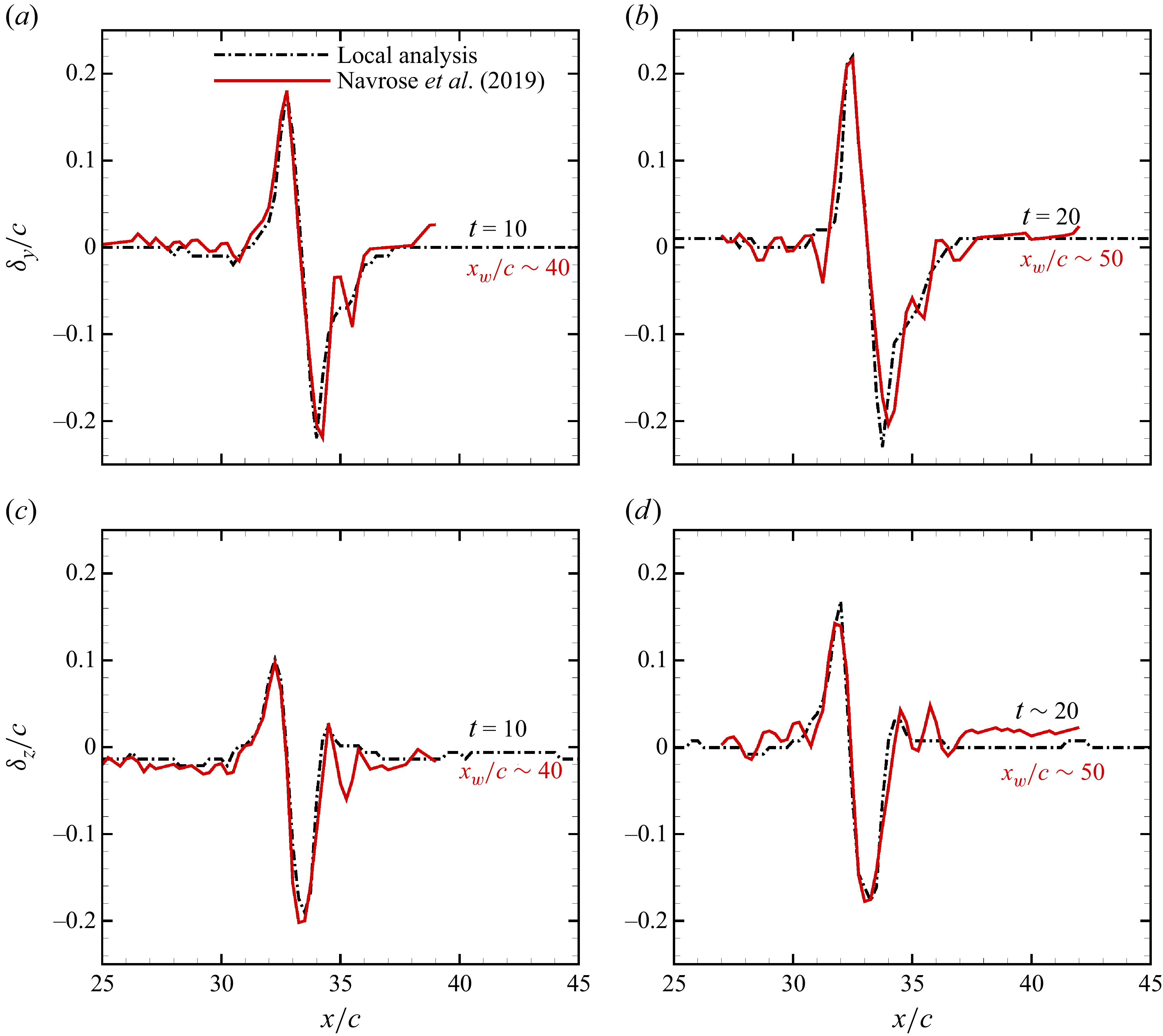
b), and is followed by gradual decay that qualitatively agrees with Navrose et al. (Reference Navrose, Brion and Jacquin2019). However, the decay rate reported by the previous study is higher than that calculated via local analysis. The difference is due to the difference in resolution of the mesh employed in the two studies. Present calculations have been carried out using a finer mesh. The results for mesh convergence are summarised in Appendix A. Despite the difference in the value of the perturbation energy between the two studies, the shape of the perturbation wavepacket (figure 10
c,d) and the deviation of the vortex centre induced by it are similar (see figure 26, Appendix A).
 ${\textit{Re}}_c=1000$
local analysis of perturbed flow. (a) Variation of energy of the perturbation wavepacket with time. For comparison, the result reported by Navrose et al. (Reference Navrose, Brion and Jacquin2019) is also included. Broken vertical line corresponds to the streamwise location
 $x_w=30c$
. (b) Zoom-in view around
 $t=0$
. (c) and (d) Structure of the perturbation wavepacket obtained via local analysis and that computed by Navrose et al. (Reference Navrose, Brion and Jacquin2019) compared at
 $t=10$
and
 $t=20$
, respectively.

The calculated perturbation energy is for the entire perturbation wavepacket. It covers TV as well as TEW. We split the energy between the two regions. This is achieved by constraining the limits of integration in (2.5) to each of the two regions. Figure 11 shows the variation of perturbation energy for TV and TEW, with time. In the initial stages of perturbation evolution, the energy is predominantly contained in TEW. With time, its energy content decreases, first gradually and steeply later on. The energy for TV, however, initially increases and then becomes nearly constant. Beyond
 $t = 300$
, the energy for the two regions are comparable. It is expected that at large times, the perturbation energy for the TV will become more dominant of the two. The results suggest that while perturbation within the TEW decays in time, that corresponding to the tip-vortex region persists far downstream of the wing. Near the wing, where TV and TEW are in the vicinity, the perturbation dynamics in the two regions is expected to be coupled. However, far downstream, TEW and TV separate (see figure 6
e), resulting in a lower interaction between the two. Consequently, far-wake perturbation dynamics of TV can reasonably be isolated from that of the remaining part of the wake.
 ${\textit{Re}}_c=1000$
local analysis of perturbed flow. (a) Variation of perturbation energy within the tip vortex (
 ) and trailing edge wake (
 ), with time. For reference, the plot for total perturbation energy (
 ) is also included. The corresponding data from Navrose et al. (Reference Navrose, Brion and Jacquin2019) are shown using hollow symbols. The inset shows the perturbation wavepacket at
 $t=375$
with the TV highlighted: (b) three-dimensional view and (c) zoom-in view in the streamwise direction.

4.3. Evolution of combined flow
As alluded to previously, the superposition of the double-helical perturbation wavepacket on the baseflow results in displacement of the tip vortex. This is in line with the observations of Jacquin et al. (Reference Jacquin, Fabre, Sipp and Coustols2005). The strength of the perturbation wavepacket, measured in terms of peak perturbation vorticity, increases from its head to mid section and then decreases towards its tail (see figure 9). Accordingly, the displacement of the vortex centre increases from head to mid-location and then decreases. Figure 12 illustrates this effect. The maximum displacement of the vortex core in this situation is
 ${\sim} 0.17c$
. Figure 13 exhibits the combined flow at different time instants of its evolution. Alongside, the co-ordinates of the vortex centre illustrating the twist of the tip vortex are shown. We define the instantaneous maximum deviation of the tip-vortex centre as
 \begin{eqnarray} {D_{\textit{max}}(t) = {\rm max}\left\{\sqrt {(y^c-y^{o})^2 + (z^c-z^{o})^2}\right\}}, \end{eqnarray}
where
 $(y^c,z^c)$
and
 $(y^{o},z^{o})$
are the co-ordinates of the vortex centre at a given streamwise location for the perturbed and unperturbed flow, respectively, and
 ${\rm max}$
denotes the maximum value function spanning all the streamwise locations. Figure 14 shows the variation of
 $D_{\textit{max}}$
with time. Also plotted is the variation of the gap between TV and TEW. It is observed that
 $D_{\textit{max}}$
increases with time, though with a diminishing growth rate. We believe that the growth rate is correlated with the coupling between TV and TEW. This, in-turn, depends on the gap between the two. A larger gap results in weaker coupling and, hence, a lower growth rate.
 ${\textit{Re}}_c=1000$
local analysis of perturbed flow. (a) Iso-surface of total vorticity (
 $|\omega |=0.025$
) and (b) co-ordinates of the vortex centre, for the initial flow. The inset in panel (b) shows the vortex displacement as viewed in the streamwise direction. The tentative location of the head and tail of the perturbation wavepacket is marked in the figures.

 ${\textit{Re}}_c=1000$
local analysis of perturbed flow: evolution of flow with time. (a,c,e,g) Iso-surface of total vorticity (
 $|\omega |=0.025$
). (b,d, f,h) Co-ordinates of vortex centre. The insets in panel (b,d, f,h) show the vortex displacement as viewed in the streamwise direction.

 ${\textit{Re}}_c=1000$
local analysis of perturbed flow. (a) Variation of maximum deviation of vortex centre from its unperturbed location, and gap between tip vortex and trailing edge wake, with time. In the inset, flow corresponding to two time instants are shown: (b,d) Iso-surface of total vorticity, (c,e) spanwise (left) and streamwise (right) vorticity in streamwise plane.

Figure 15 shows streamwise variation of spanwise and vertical position of the tip-vortex centre at different instants of time. With time, the perturbation wavepacket spreads in the streamwise direction. The approximate extent of the perturbation wavepacket is highlighted in the figure. We have marked streamwise locations that correspond to a similar phase across different time instants. For example, the blue and red markers correspond to a pair of adjacent peak and valley identified in the spanwise displacement plots. The markers and shaded region suggest that the speed of the perturbation wavepacket is small but non-zero and it moves towards the left boundary. We recall that the calculations are carried out in the frame of reference that is moving with the free stream speed. The speed of the perturbation wavepacket, therefore, is slightly lower than the free stream speed. The streamwise extent of the perturbation grows from approximately
 $5c$
to
 $17c$
in
 $400$
time units (see figure 15
a). It is likely that in due course of time, the perturbation wavepackets disperse to an extent that they start interacting with each other. We discuss such interactions in the next section.
 ${\textit{Re}}_c=1000$
local analysis of perturbed flow. Streamwise variation of (a) spanwise and (b) vertical position of the vortex centre. Time is indicated on each plot. Plots in panel (a) have been shifted for better illustration. The shaded region highlights the approximate extent of the perturbation wavepacket. The colour-coded solid circles correspond to the same phase at different time instants.

4.4. Effect of spacing between perturbation wavepackets
The results presented in the preceding sections are for the situation when the average spacing between two successive perturbation wavepackets is
 $44c$
. Reducing the spacing between the perturbation wavepackets is tantamount to increasing the frequency of injection of optimal perturbation. The variation of spacing can be carried out by either reducing the streamwise extent of the computational domain or by adding more perturbation wavepackets to the baseflow while keeping the same streamwise extent of the domain. We employ the latter. Two situations, denoted in the following as 2X and 3X, are considered. In 2X, two equi-spaced perturbation wavepackets are added to the baseflow. Similarly, for 3X, three equi-spaced perturbation wavepackets are added. In both the set-ups, the initial spacing between the perturbation wavepackets is adequately large to avoid any interaction between them. As the number of perturbation wavepackets increase, the chances of nonlinear interaction between them increases, which in-turn, renders the initial linear superposition invalid.
Figure 16(a) shows the streamwise perturbation vorticity at
 $t=0$
. The evolution of the combined flow is shown in panels (b)–(e). For reference, we have added the results of the preceding section, denoted as 1X, in the first column of the figure. It is observed that the effect of perturbation wavepacket(s) is similar in all the three situations. They result in a helical twist of the vortex core. Within the trailing edge wake, semi-ring structures are identified.
 ${\textit{Re}}_c=1000$
local analysis of perturbed flow. Evolution of flow for different frequencies of injection of optimal perturbation. (a) Streamwise vorticity of the perturbation (
 $\omega _x=\pm 0.01$
) at
 $t=0$
. (b–e) Total vorticity (
 $|\omega |=0.025$
) of the combined flow. The first, second and third columns correspond to 1X, 2X and 3X simulation, respectively.

Figure 17 shows the streamwise variation of the spanwise and vertical position of the vortex centre at different time instants for 3X. The initial evolution of each perturbation wavepacket is the same as 1X. With time, the perturbation wavepackets disperse in the streamwise direction and beyond
 $t \sim 250$
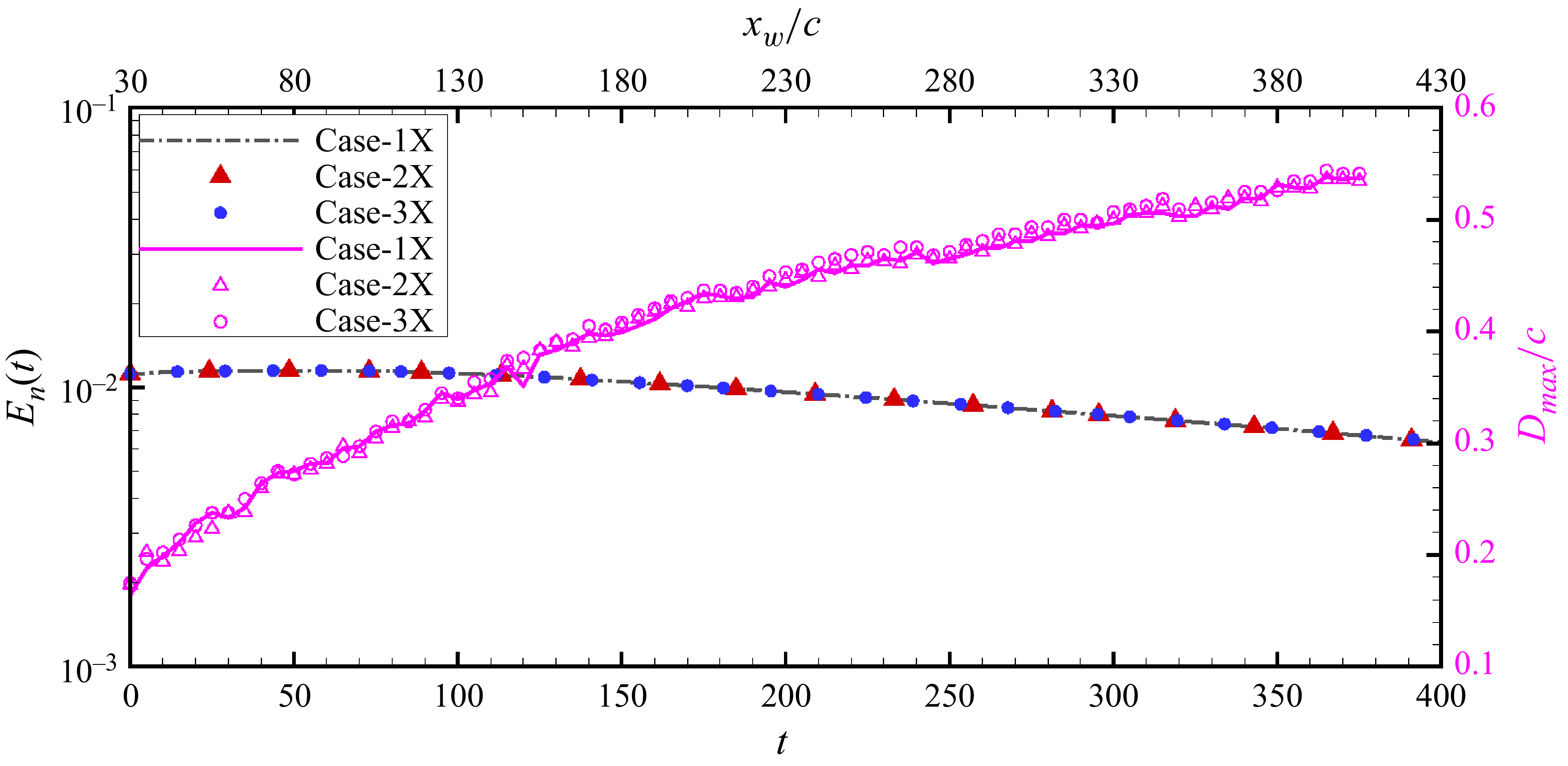
, they interact. The interaction, however, has negligible effect on the maximum deviation of the vortex core and normalised perturbation energy. This is evident from figure 18, where we have plotted the variation of the two with time. The plots for 1X, 2X and 3X nearly overlap. Here, the normalised perturbation energy (
 $E_n$
) is defined as the perturbation energy per wavepacket.
 ${\textit{Re}}_c=1000$
local analysis of perturbed flow. Streamwise variation of (a) spanwise and (b) vertical position of the vortex centre for 3X simulation. Time is indicated on each plot. Plots in panel (a) have been shifted for better illustration.

 ${\textit{Re}}_c=1000$
local analysis of perturbed flow. Variation of perturbation energy (solid symbols) and maximum deviation of vortex centre (hollow symbols), with time, for different frequencies of injection of optimal perturbation. For reference, the plots for 1X simulation are shown using a line, broken for energy and solid for maximum deviation.

Model analysis of perturbed flow
 $a/b=0.18$
,
 ${\textit{Re}}_\varGamma = 1000$
. Flow evolution shown using iso-surface of total vorticity. For better illustration, the flow has been extended in the streamwise direction by one period and vortices are coloured differently: red for counter-clockwise and blue for clockwise vortex. The extension is highlighted in panel (a) that shows the flow at
 $t=0$
. The first, second and third columns show the three-dimensional, top and side-view, respectively.

Model analysis of perturbed flow
 $a/b=0.18$
,
 ${\textit{Re}}_\varGamma = 1000$
. Variation of maximum deviation of vortex centre with time. Exponential fit to the data points is shown using dash-dotted line Time at which the two vortices come in contact is indicated with a vertical broken line. Beyond this, vortex-linking starts (shaded region) resulting in the formation of vortex rings. In the inset, helical perturbation is shown at two different time instants.

The results of local analysis presented previously suggest that the perturbation wavepacket maintains its structure in the tip vortex far downstream of the wing. Despite the perturbation wavepacket inducing maximum displacement of
 ${\sim} 0.5c$
, there is no evidence of instability of the vortex pair. The reason is attributed to low
 ${\textit{Re}}_\varGamma$
and relatively large separation between the counter-rotating vortices. For local analysis,
 ${\textit{Re}}_\varGamma = 27$
. In general, the growth rate of the instability increases with increase in
 ${\textit{Re}}_\varGamma$
. Further, for a counter-rotating vortex pair, the growth rate scales inversely with the separation distance,
 $b$
(Crow Reference Crow1970; Saffman Reference Saffman1992; Leweke & Williamson Reference Leweke and Williamson2011). In the following, we investigate the effect of
 ${\textit{Re}}_\varGamma$
and
 $b$
. We carry out calculations using a different set-up where the flow comprises a pair of counter-rotating vortices only and the trailing edge wake is absent. This emulates the far-wake TV dynamics that is decoupled from TEW. The analysis has been referred to as model analysis since
 $q$
-vortex is used to model the tip vortex. The set-up allows flexibility in terms of variation of
 ${\textit{Re}}_\varGamma$
,
 $b$
and other vortex parameters while keeping computational cost at a reasonable level.
5. Model analysis
The baseflow consists of a counter-rotating vortex pair. Each vortex in the pair is modelled as a well-known
 $q$
-vortex with equal strength. A
 $q$
-vortex is an axisymmetric vortex, and is completely described by its radius (
 $a$
), circulation (
 $\varGamma$
) and axial velocity deficit at the vortex centre (
 $\gamma$
). The deficit is with respect to the free stream speed. The velocity distribution for the
 $q$
-vortex is given by
 \begin{eqnarray} U_{\theta } = {\frac {\varGamma }{2\pi r U_\infty } \left ( 1-e^{-r^2/a^2} \right )},\def\lumina\hspace {0.5cm} U_r = 0, \def\lumina\hspace {0.5cm} U_x = {1-\frac {\gamma }{U_\infty } e^{-r^2/a^2}}. \end{eqnarray}
In (5.1), the velocity components have been expressed in a cylindrical co-ordinate system whose origin coincides with the vortex centre;
 $U_{\theta }$
,
 $U_r$
and
 $U_x$
are the azimuthal, radial and axial component of the velocity, respectively. The radial distance from the vortex centre has been denoted by
 $r$
.
Model analysis of perturbed flow
 $a/b=0.18$
,
 ${\textit{Re}}_\varGamma = 1000$
: effect of Reynolds number (columns I and II), and effect of initial perturbation energy (columns III and IV). Columns I and III show the flow at
 $t=0$
. Columns II and IV show the flow at a time instant around vortex contact.
 ${\textit{Re}}_\varGamma$
decreases from top to bottom in I and II. Similarly,
 $E(0)$
decreases from top to bottom in III and IV. For better illustration, the flow has been extended in the streamwise direction by one period and vortices are coloured differently: red for counter-clockwise and blue for clockwise vortex.

Model analysis of perturbed flow
 $a/b=0.18$
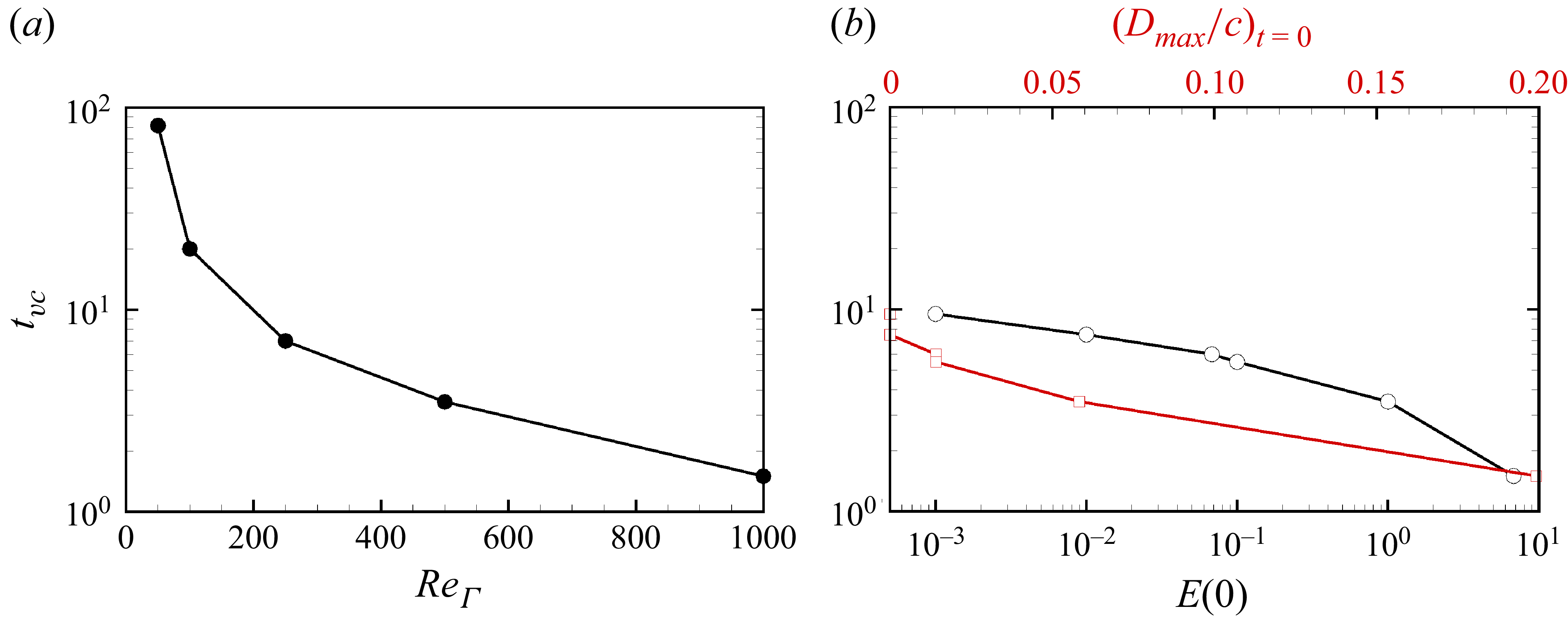
. Variation of vortex-contact time with (a) Reynolds number and (b) initial energy of the perturbation and corresponding initial maximum deviation for
 ${\textit{Re}}_\varGamma =1000$
.

Model analysis of perturbed flow
 $a/b=0.18$
,
 ${\textit{Re}}_\varGamma = 1000$
. Streamwise variation of (a) spanwise and (b) vertical position of vortex centre at
 $t=0$
for different
 $E(0)$
.

Model analysis of perturbed flow
 $a/b=0.18$
,
 ${\textit{Re}}_\varGamma = 1000$
. Variation of maximum deviation of vortex centre with time. The initial energy of the perturbation is
 $E(0)=10^{-3}$
. Exponential fit to the data points is shown using dash-dotted line. The time instant around which vortices come in contact is shown using a vertical broken line. Also shown as insets are the flow at different instants of time.

5.1. Effect of vortex parameters and perturbation strength
We investigate the effect of vortex parameters on the dynamics of the perturbed vortex pair and explore if optimal perturbation can indeed be effective in hastening the onset of instability. The counter-rotating
 $q$
-vortex pair is perturbed by giving a localised helical twist. The deformed flow is shown in figure 19(a). The helical twist closely models the deformation induced by the perturbation wavepacket in the wing simulation (see Appendix B). As for the local analysis, the evolution of the perturbed flow is studied in a reference frame that moves with the free stream speed. In earlier studies (Brion Reference Brion2009; Johnson et al. Reference Johnson, Brion and Jacquin2016; Navrose et al. Reference Navrose, Johnson, Brion, Jacquin and Robinet2018), the perturbation is added after the initial adjustment of the vortex pair. However, in the present work, we add the perturbation at
 $t=0$
. This is carried out for the ease in giving the localised helical twist over a wide parametric space that is explored. It is shown in Appendix C that the qualitative evolution of the perturbation, especially with regards to the deviation of the vortex centre from its unperturbed location is relatively unaffected by the initial adjustment.
5.1.1. Vortex Reynolds number
 ${\textit{Re}}_\varGamma$

Johnson et al. (Reference Johnson, Brion and Jacquin2016) studied the growth of instability in a
 ${\textit{Re}}_{\varGamma }=1000$
counter-rotating Lamb–Oseen vortex pair for different strength of the initial perturbation. We use similar vortex parameters as them. Accordingly,
 $a=0.18c$
and
 $b=1c$
. The axial velocity deficit of the
 $q$
-vortex is set to
 $0.05U_\infty$
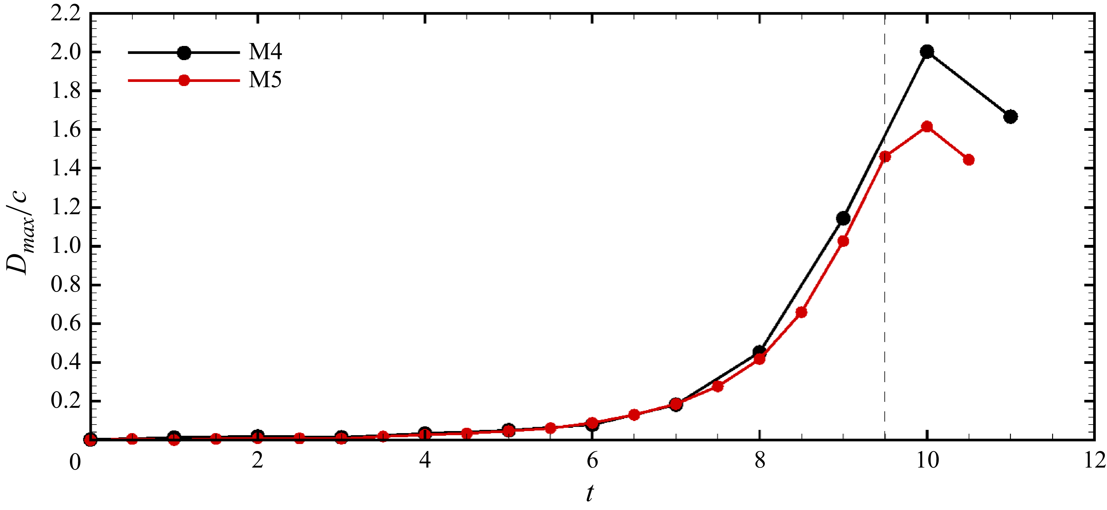
. It is observed that the localised helical twist results in an instability that resembles the Crow instability. Figure 19 illustrates the flow at different time instants of its evolution. As the disturbance grows, the deviation of the vortex centre from its unperturbed position increases. The maximum deviation increases with time as illustrated in figure 20. At
 $t \sim 1.5$
, the vortex columns come in contact with each other. Subsequently, the vortices start to diffuse into each other resulting in the formation of a vortex ring. Before the vortices come in contact, they are nearly planar. After coming in contact, significant out of plane deformation occurs (see the last column of figure 19).
We recall that for the local analysis
 ${\textit{Re}}_\varGamma \sim 27$
. The above analysis suggests that the Reynolds number (
 ${\textit{Re}}_\varGamma$
) has a significant effect on the evolution of a vortex pair with helical twist disturbance. While the disturbance seems benign for exciting instability at low
 ${\textit{Re}}_\varGamma$
, it results in the formation of vortex rings at large
 ${\textit{Re}}_\varGamma$
. We carry out calculations for various
 ${\textit{Re}}_\varGamma$
in the range
 $27{-}1000$
. The results are illustrated in the first two columns of figure 21. The first column shows the initial flow field and the second column shows the flow at a later time. In situations where the vortex columns come into contact with each other (
 ${\textit{Re}}_\varGamma \geqslant 50$
), the images in the second column correspond to the time instant of contact. It is observed that with an increase in
 ${\textit{Re}}_\varGamma$
, the time for vortex-contact decreases (figure 22
a). Additionally, the critical
 ${\textit{Re}}_\varGamma$
for the helical twist to result in a vortex contact is between
 $27 \lt {\textit{Re}}_{\varGamma _{cr}} \lt 50$
.
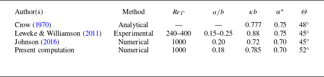
Comparison of wavelength of perturbation (
 $\kappa b$
,
 $\kappa$
is wavenumber), growth rate of instability (
 $\alpha ^*$
) and inclination of the deformation plane (
 $\varTheta$
) obtained in the present study with earlier works.

5.1.2. Amplitude of initial disturbance
In the preceding analyses, the initial perturbation is such that the vortex core displaces by the same amount for all
 ${\textit{Re}}_\varGamma$
. The strength of the perturbation, measured in terms of perturbation energy, increases with an increase in
 ${\textit{Re}}_\varGamma$
. We investigate the effect of the initial perturbation energy,
 $E(0)$
, on the flow evolution while fixing
 ${\textit{Re}}_\varGamma =1000$
. Figure 23 shows the spanwise and vertical co-ordinates of the perturbed vortex for various
 $E(0)$
. The corresponding flow is shown in the third column of figure 21. For
 $E(0)=10^{-3}$
, the lowest value of
 $E(0)$
, the deviation of the vortex centre at
 $t=0$
is imperceptible. It increases with increase in
 $E(0)$
. As the perturbed flow evolves, deviations increase with time, leading to vortex contact. This can be observed in the fourth column of figure 21. We investigate the results of
 $E(0)=10^{-3}$
simulation in detail. This situation corresponds to a weak initial disturbance. As such, the growth of the perturbation, during initial stages, follows linear evolution. Figure 24 shows the variation of the maximum deviation (
 $D_{\textit{max}}$
) of the vortex centre with time. The data points have been fitted to a least squares exponential curve. In the initial stages, the maximum deviation increases exponentially with a growth rate of
 $\alpha ^*=0.70$
until
 $t\sim 8$
. The value of the growth rate is in very good agreement with the growth rate of Crow instability in the literature (see table 1) for similar vortex parameters. The deformation of the vortices occur in a plane that is aligned at an angle of
 $52^{\circ }$
, which is reasonably close to the inclination of Crow instability reported by Crow (Reference Crow1970). Further, the Fourier decomposition of the flow data yields that the most dominant mode has an axial wavenumber of
 $8b$
. These observations affirm that the helical perturbation is effective in exciting Crow instability. At large time, the maximum-deviation data points deviate from the exponential curve owing to nonlinear processes. Johnson et al. (Reference Johnson, Brion and Jacquin2016) showed that the vortex linking for a weak disturbance occurs at
 $t\sim 9$
. This matches well with our computation where linking is observed at
 $t\sim 9.5$
. The time for vortex contact,
 $t_{vc}$
, is found to decrease with increase in
 $E(0)$
and corresponding maximum deviation
 $D_{\textit{max}}$
at
 $t=0$
(figure 22
b).
6. Summary and conclusions
The present study is a part of an ongoing work on mitigating the chances of wake vortex encounter. Earlier work by Navrose et al. (Reference Navrose, Brion and Jacquin2019) showed that the linear optimal perturbation for the flow past a finite span wing is located in the vicinity of the wing and is associated with a large gain of perturbation energy. The linear optimal perturbation evolves as a downstream travelling perturbation wavepacket with speed nearly the same as the free stream speed, and its energy and shape do not change significantly beyond a certain downstream distance. The perturbation wavepacket has a double-helical structure within the tip vortex and induces a helical twist to it. Though Navrose et al. (Reference Navrose, Brion and Jacquin2019) had surmised that LOP can be effective for reducing the lifespan of vortices, it was not definitively established owing to constraint of the downstream extent of the computational domain which was
 ${\sim} 60c$
. Here, we have studied the effect of LOP further downstream and in the far wake. The LOP is injected periodically in the flow. The investigation is carried out in a frame of reference that moves with the free stream speed. Two approaches have been used: local analysis and model analysis. The former mimics the wake structure for intermediate distances from the wing (
 $60c \lesssim x_w \lesssim 400c$
) wherein both trailing edge wake and tip vortices are present. In the model approach, only the tip vortices are considered and this is expected to model the vortex dynamics beyond
 ${\sim} 400c$
. The results for the two approaches are summarised here.
The evolution of unperturbed flow predicted by local analysis for
 $x_w \leqslant 60c$
is found to be in very good agreement with the results of wing simulation by Navrose et al. (Reference Navrose, Brion and Jacquin2019). Further calculations for the unperturbed flow suggest that it does not develop instability even far downstream of the wake (
 $x_w \sim 400c$
). For the perturbed flow, we find that the double-helical structure of the perturbation wavepacket is preserved within the tip vortex and its strength remains nearly constant. The perturbation energy content of the trailing edge wake, however, is found to decrease with downstream distance. The displacement of the wing-tip vortex, owing to the double helical perturbation, increases steeply with
 $x_w$
initially and tends towards saturation further downstream. We suspect that the latter evolution is due to widening of the gap between the tip vortex and trailing edge wake with downstream distance. The proximity of the two flow regions appears to be conducive to the growth of tip-vortex perturbation energy. We have also explored the effect of frequency of injection of LOP in to the flow. At high frequency, the perturbation wavepackets, though initially separated, interact with each other further downstream owing to slow dispersion of the perturbation wavepackets in the streamwise direction. The interaction, however, does not have any effect on the maximum deviation of the vortex core. Like the unperturbed flow, the perturbed flow also does not exhibit instability.
In the model analysis, the tip vortex is modelled as a
 $q$
-vortex. The model analysis provides more flexibility in terms of variation of vortex parameters, thereby allowing greater exploration of the parameter space. The vortices are perturbed with double-helical perturbation, resembling the shape of the perturbation wavepacket in wing simulation. To promote the growth of instability, we have decreased the vortex spacing and increased the Reynolds number (
 ${\textit{Re}}_\varGamma$
) of the vortex pair. The vortex pair develops instability, reminiscent of Crow instability (Crow Reference Crow1971). As the instability grows, the vortices come in contact with each other resulting in the formation of vortex rings. The time for vortex contact (
 $t_{vc}$
) decreases with increase in
 ${\textit{Re}}_\varGamma$
. Our calculations suggest that the critical
 ${\textit{Re}}_\varGamma$
for the onset of instability is between
 $27$
and
 $50$
. For a fixed
 ${\textit{Re}}_\varGamma$
,
 $t_{vc}$
decreases with increase in the strength of the initial perturbation. We expect that the reduction in
 $t_{vc}$
will translate to a lower lifespan of the wing-tip vortices.
Our present effort has shown that linear optimal perturbation for the flow past a finite span wing is promising from the perspective of controlling the lifespan of wing-tip vortices, thereby reducing the chances of wake–vortex encounter. Since the general shape of the optimal perturbation is agnostic to the variation of Reynolds number, aspect ratio and angle of attack, the inferences drawn in the present work can be extended over a large parameter space. For example, an Airbus A380 at cruise generates a tip-vortex pair with
 $a/b\approx 0.044$
,
 $b\approx 63{\,}{\rm m}$
and
 $\varGamma \approx 900{\,\rm m^2\,s^{- 1}}$
. The resulting value of
 ${\textit{Re}}_\varGamma \approx O(10^6)$
(Rojas, Melgosa & Prats Reference Rojas, Melgosa and Prats2021). We extrapolate our results as shown in figure 22(a) to estimate
 $t_{vc}$
. The predicted value is
 $t_{vc}\approx 7\times 10^{-4}$
. The corresponding time in seconds is
 $0.021{\,}{\rm s}$
which, based on our low
 $Re$
results, is expected to be smaller than that of the unperturbed vortex system. The control via LOP, therefore, appears promising for reduction of vortex lifespan.
An interesting perspective of our work could be on understanding the mechanism underlying the phenomenon of vortex meandering – a seemingly random motion of wing-tip vortex observed in wind-tunnel experiments. Navrose et al. (Reference Navrose, Brion and Jacquin2019) surmised that the near-wake energy amplification and nonlinear effects might be central to vortex meandering. The results of local and model analysis suggest that the proximity of the trailing edge wake to the tip vortex in the near-wake region may be responsible for the increase in the maximum deviation of the perturbed tip vortices. This seems to agree well with experimental observations that vortex meandering generally increases up to a short distance from the wings. Therefore, in addition to external turbulence, trailing edge wake dynamics could also be significant in vortex meandering.
Acknowledgements
We acknowledge the use of computational resources at High-Performance Computing (HPC) and PARAM Sanganak facilities set up under the aegis of the Department of Science and Technology (DST) and the National Supercomputing Mission(NSM), Government of India at the Indian Institute of Technology, Kanpur.
Declaration of interests
The authors report no conflict of interest.
Appendix A. Mesh details, convergence study and comparison with wing simulation data
A.1. Local analysis
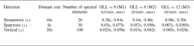
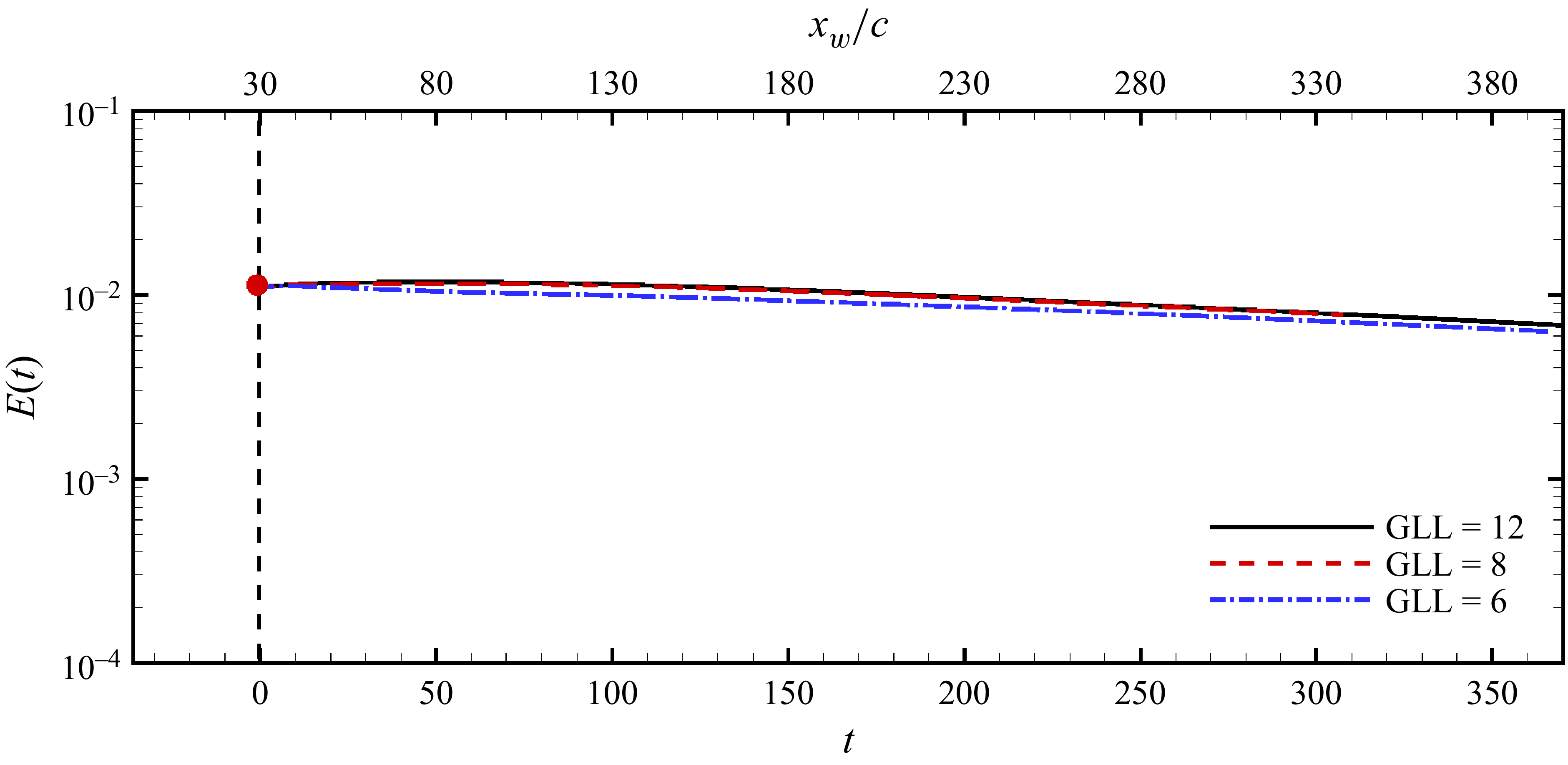
Table 2 lists the details regarding domain size and mesh employed for local analysis. Three meshes were used for calculations and showing convergence of results. The meshes were obtained by varying the number of GLL points within the spectral element; more GLL points corresponds to a finer mesh. To establish the adequacy of the mesh used for local analysis, we compare the energy of the perturbation wavepacket (
 $E(t)$
) obtained via simulations carried out with mesh M1, M2 and M3. Figure 25 illustrates the evolution of perturbation energy (
 $E(t)$
) with time (
 $t$
) for the three meshes. The maximum difference in the perturbation energy between M2 and M3 is
 ${\sim} 2\,\%$
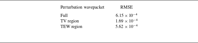
. We have used the computational data obtained using M3 for presenting most of the results in this work. An important question around the local analysis is its efficacy in predicting the results of wing simulation. Table 3 quantifies the difference between datasets shown in figures 10 and 11 using RMSE (root mean square error). Perturbation energy comparison is done for a full perturbation wavepacket as well as the TV and TEW region. For all cases, RMSE
 $\sim O(10^{-4})$
. The mesh resolution effect is dominant in the TEW region and least in the TV region, likely due to the fact that Navrose et al. (Reference Navrose, Brion and Jacquin2019) have employed a finer mesh in the TV region as compared with the TEW region, whereas the present results consider uniform mesh throughout the domain. Earlier in the paper, we had compared the structure of the perturbation wavepacket obtained from the local analysis and wing simulation, and show that they are in good agreement. Here, we further support our claim by showing comparison of the deviation of the vortex centre in the spanwise (
 $\delta _y$
) and vertical (
 $\delta _z$
) direction at two time instants after the perturbation wavepacket has been added (see figure 26). The results of local analysis matches reasonably with wing simulation.
Details of the domain size and mesh employed for local-analysis.
 $\Delta l(\textit{min},\textit{max})$
denotes the minimum and maximum grid spacing in the corresponding direction. GLL is the number of Gauss–Lobato–Legendre points inside each spectral element.

Comparison of the perturbation wavepacket energy data obtained through local analysis with results of Navrose et al. (Reference Navrose, Brion and Jacquin2019).

 ${\textit{Re}}_c=1000$
local analysis of perturbed flow. Effect of mesh resolution on energy of the perturbation wavepacket.

 ${\textit{Re}}_c=1000$
local analysis of perturbed flow. Comparison with simulation of Navrose et al. (Reference Navrose, Brion and Jacquin2019) at two time instants. (a,b) Spanwise deviation and (c,d) vertical deviation.

A.2. Model analysis
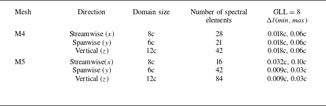
For the model analysis, calculations were carried out for two meshes of different resolutions. The details of the mesh are listed in table 4. Figure 27 shows the maximum deviation of the vortex centre for simulations initiated with helical-twist disturbance for the two meshes. The results are in good agreement. The vortex contact occurs at
 $t\sim 9.5$
and the deformation plane is inclined at
 $\varTheta =52^\circ$
.
Details of the domain size and mesh employed for model analysis.
 $\Delta l(\textit{min},\textit{max})$
denotes the minimum and maximum grid spacing in the corresponding direction. GLL is the number of Gauss–Lobato–Legendre points inside each spectral element.

Model analysis of perturbed flow
 $a/b=0.18$
,
 ${\textit{Re}}_\varGamma = 1000$
and
 $E(0)=10^{-3}$
. Effect of mesh resolution on maximum deviation of the vortex centre.

(a) Spanwise and (b) vertical deviation of vortex centre when the perturbation wavepacket is located at
 $x_w=30c$
,
 $40c$
and
 $50c$
in wing simulation (Navrose et al. Reference Navrose, Brion and Jacquin2019). The deviation corresponding to the helical-twist perturbation used in model analysis is also included in the figure. (c) Illustration of vortex with (red) and without (black) the helical twist.

Appendix B. Helical-twist disturbance
Our results for local analysis shows that the disturbance induced by the perturbation wavepacket remains largely similar and resemble a localised helical twist (figure 1). Figure 28 shows the spanwise and vertical deviation of the vortex centre at three streamwise locations for the wing simulation clearly illustrating the aforementioned similarity. The streamwise axis has been shifted for each case accordingly to facilitate comparison. We model the helical twist by fitting the data points to a piecewise cubic spline. The cubic spline then is used to shift the centre of CRQV to create the helical twist (figure 28 c) that serves as the initial perturbation for the model analysis. The corresponding spanwise and vertical deviation is shown in figure 28(a,b).
Appendix C. How important is the initial adjustment of CRQV?
Model analysis of unperturbed flow. Variation of aspect ratio of vortex in CRQV pair with time for
 ${\textit{Re}}_\varGamma =27$
and
 ${\textit{Re}}_\varGamma =250$
(in inset). The shaded region in each denotes the time interval corresponding to initial adjustment of the vortex (Brion Reference Brion2009; Johnson et al. Reference Johnson, Brion and Jacquin2016).

Model analysis of the perturbed flow
 ${\textit{Re}}_\varGamma =27$
. Comparison of maximum deviation of the vortex centre with simulation that takes into account the initial adjustment of CRQV.

Model analysis of perturbed flow
 ${\textit{Re}}_\varGamma =250$
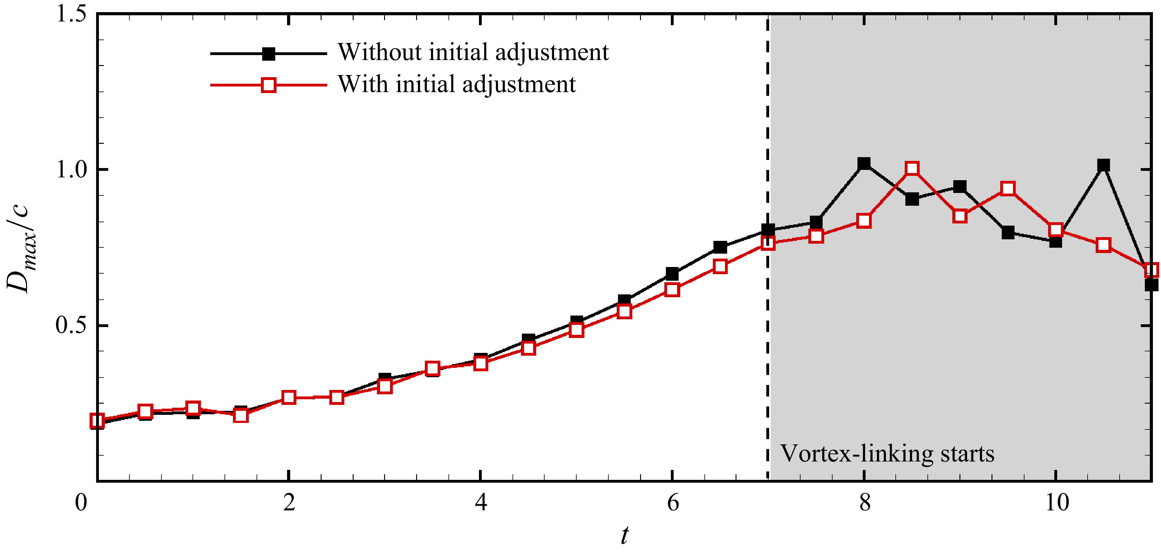
. Comparison of maximum deviation of the vortex centre with simulation that takes into account the initial adjustment of CRQV. The time instant around which the vortices come into account is marked with a vertical broken line. Beyond this, vortex linking starts, eventually resulting in the formation of vortex rings.

A counter-rotating
 $q$
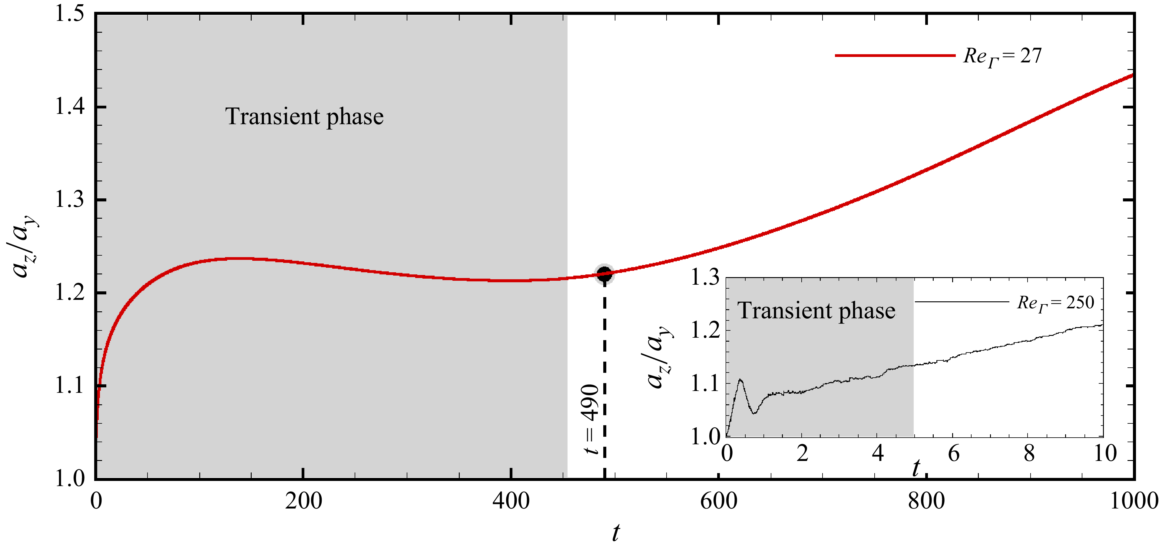
-vortex pair is not a solution of Navier–Stokes equation. Earlier studies using such a pair have employed an approach wherein the initial flow comprising CRQV is time-stepped forward for some time for the flow to adjust to the governing equations (Sipp Reference Sipp1999; Brion, Sipp & Jacquin Reference Brion, Sipp and Jacquin2007; Johnson et al. Reference Johnson, Brion and Jacquin2016). The adjustment is analysed in terms of the aspect ratio (
 $a_z/a_y$
) of the vortices, where
 $a_z$
and
 $a_y$
represent the semi-widths of the vortices in the
 $z$
and
 $y$
directions, respectively. These are defined as
 \begin{eqnarray} {a_{z,y}^2\varGamma = \int _{\varOmega _{TV}} (z,y-z^{\circ},y^{\circ})^2 \omega _x \, {\rm d}\varOmega }, \end{eqnarray}
where
 $\varGamma$
is the circulation,
 $\omega _x$
is the axial-vorticity, and
 $(z^{\circ}, y^{\circ})$
are the vortex centre coordinates in the
 $z$
and
 $y$
directions, respectively. During the adjustment, the aspect ratio of the vortex changes non-monotonically with time. After the vortices have adjusted, the increase is monotonic and gradual. In the present work, we have added the helical-twist perturbation to the CRQV directly. A question that arises is how important is the adjustment of CRQV in the context of present work. We explored this for two values of
 ${\textit{Re}}_\varGamma$
. To this end, we time evolve the CRQV so that it adjusts. Figure 29 shows the evolution of the aspect ratio of vortex with time. It is observed that for
 ${\textit{Re}}_\varGamma = 27$
beyond
 $t=490$
, the variation of the vortex aspect ratio is monotonic. We take the evolved vortex pair at
 $t=490$
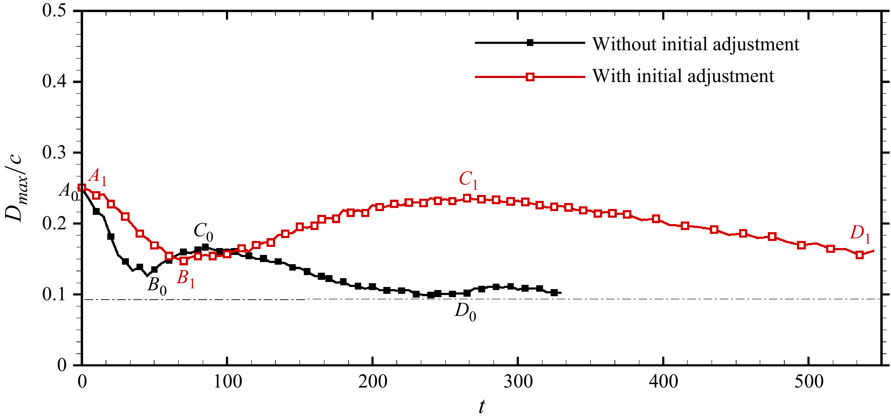
and add the helical-twist perturbation. Figure 30 shows the time evolution of the maximum deviation (
 $D_{\textit{max}}$
) of the vortex centre. Also plotted are the results from model analysis. The two evolutions are in qualitative agreement:
 $D_{\textit{max}}$
initially decreases, increases for some time and then decreases before tending towards saturation. The quantitative difference is attributed to significant increase in the size of the vortex during the adjustment phase. If we increase the Reynolds number (
 ${\textit{Re}}_\varGamma$
), the results of model analysis matches very well with those obtained using adjusted CRQV, as shown in figure 31.