





Highlights
What is already known?
-
• Meta-analytic structural equation modeling (MASEM) is a flexible framework for testing hypothesized structural equation models using meta-analytically pooled correlation matrix.
-
• Despite MASEM’s benefits, several methodological challenges remain, including: (1) handling within-study variability in moderators hypothesized as the source of variability in relationships among variables in the structural equation model and (2) any kind of within-study dependence in correlation estimates and correlation matrix multiplicity.
-
• Within-study variability in moderators is also often handled in ad hoc ways in MASEM, including deletion or aggregation methods that unnecessarily negatively narrowing the resulting moderator analysis inferences.
-
• Several types of within-study dependence are common among correlations being pooled for MASEM. However, little research has focused on primary studies’ reporting multiple estimates of the same correlation in a matrix using the same sample with a lack of methodological demonstrations for how to handle this dependence in MASEM.
What is new?
-
• We propose adding an extension (“Stage 0”) to the typical two stages of MASEM that incorporates categorical moderators directly into the hypothesized structural equation model.
-
• We demonstrate how to integrate robust variance estimation (RVE) combined with a three-level multivariate meta-regression model when pooling correlation matrices to handle any type of remaining within-study dependence in the correlation estimates being pooled.
-
• To test hypotheses about differences in structural equation model parameters as a function of moderator variable values, we demonstrate how to specify the relevant MASEM models and two methods for testing the moderator’s effect, including: (1) model comparison using the likelihood ratio test and (2) direct path-difference estimation using log-likelihood-based confidence intervals.
Potential impact for RSM readers
-
• We provide a robust methodological framework and practical guidance for moderator analyses in MASEM, broadening the flexibility of MASEM’s use.
-
• We demonstrate how to implement multilevel multivariate modeling with RVE as one method to handle complex effect size multiplicity within the two-stage MASEM workflow using readily available R packages and reproducible code.
-
• We offer three illustrative examples with diverse structural equation model formulations and corresponding R code that meta-analysts can adapt for their own research.
1 Introduction
For meta-analysts interested in the relationships between two interval- or ratio-scaled variables (or constructs), the associated focal effect size metric is the Pearson correlation coefficient. For example, Seoane et al.Reference Seoane, Wang, Cao and Kim 1 aimed to understand the relationship between oral language and written composition and factors that might influence that correlation. A standard meta-analysis can use the correlation coefficient as the effect size of interest which allows pooling of the correlation estimates and assessing the extent to which study and sample descriptors explain heterogeneity in the correlation estimates.
Meta-analysts may wish to expand their research questions beyond the relationship between a pair of variables and investigate more complex relationships among multiple variables. For this purpose, meta-analytic structural equation modeling (MASEM) offers a useful method. MASEM is a flexible modeling framework that combines the benefits of meta-analysis for pooling information across studies with the flexibility of the structural equation modeling (SEM) framework.Reference Cheung 2 , Reference Jak 3 Using meta-analytic techniques, the researcher can pool estimates of the correlation between each bivariate relationship in the hypothesized structural equation model and obtain a pooled correlation matrix that is based on a larger sample (from across the primary studies) than would be used in a single primary study. In addition, due to the ability to use correlations from across primary studies, the meta-analyst can explore whether study or sample characteristics are associated with differences in SEM parameters. The MASEM researcher can test the same kinds of models as in conventional SEM, including path models, factor models, and structural models with mediators and moderators. The SEM estimation allows testing of hypotheses about model parameters, model fit, and model fit comparison.
To conduct research utilizing MASEM, a researcher would first identify and determine key constructs (variables) and hypothesize relationships among them in the form of a structural equation model. Then, the researcher builds the meta-analytic dataset from primary studies that report estimates of correlations among any of the pairs of variables to construct the correlation matrix of interest. Once the meta-analytic dataset of correlation estimates is created, different MASEM approaches can be employed, including two-stage MASEM (TS-MASEM) and one-stage MASEM (OS-MASEM).Reference Jak and Cheung 4
With TS-MASEM, the pooling of the correlation matrix (stage one) and fitting of the structural equation model (stage two) are conducted separately. The correlations from different primary studies are synthesized to provide the pooled correlation matrix,
$\boldsymbol {R.}$
 and its associated covariance matrix,
$\boldsymbol {V_{R.}}$
 , is also estimated in stage one. The covariance matrix (
$\boldsymbol {V_{R.}}$
 ) for the vector of pooled correlations contains the (inverse of the) precisions of each pooled correlation which are used as weights when estimating the structural equation model in stage-two of TS-MASEM. Cheung and Chan introduced a specific technique for the TS-MASEM framework that they termed two-stage structural equation modeling.Reference Cheung and Chan
5
Their estimation procedure used for stage one of TS-MASEM offers one option for pooling correlation estimates across studies. We will use the term tssem1 to specifically represent Cheung and Chan’s method for conducting stage one of TS-MASEM.Footnote
i
,
Reference Cheung and Chan
5
In the current study, we review other options and demonstrate an alternative for pooling correlation matrix elements and obtaining the matrix’s covariance matrix in stage one of TS-MASEM.
OS-MASEM achieves the same goal as TS-MASEM, although in a single “stage.” With OS-MASEM, there is no separation of the MASEM process into two stages and instead the primary studies’ correlations are directly used to estimate the structural equation model. More details about the different MASEM approaches are laid out well in prior research.Reference Cheung 2 , Reference Jak and Cheung 4 , Reference Viswesvaran and Ones 7
While MASEM offers a flexible framework for investigating nuanced relations among multiple variables simultaneously, several methodological challenges remain. In this study, we focus on two main methodological considerations when modeling and estimating MASEM in practice, including: (1) handling within-study variability in categorical moderators that are hypothesized to explain heterogeneity in SEM parameters and (2) handling within-study dependence in effect sizes (here, correlations).
We first conceptualize and review the above two challenges within the general TS-MASEM framework as we discuss the current practices used when handling the two challenges. We then present our proposed approach for tackling each challenge by adapting the two-stage procedure to conduct MASEM, with a foundation in Cheung and Chan’s approach.Reference Cheung and Chan 5 In sum, we propose a modeling approach that can incorporate categorical within-study moderators while accounting for any kind of within-study dependence in correlations, using, for example, multilevel multivariate modeling with robust variance estimation (RVE).Reference Hedges, Tipton and Johnson 8 , Reference Pustejovsky and Tipton 9 We demonstrate the proposed approach using illustrative examples with several different structural equation models. After summarizing the proposed procedures, we also discuss some practical considerations for MASEM researchers, limitations of the current study, and directions for future research.
2 Moderators in MASEM
In addition to pooling effect size estimates, assessment of the extent to which moderating study and sample characteristic variables explain variability in effect sizes offers an important purpose for meta-analysis.Reference Tipton, Pustejovsky and Ahmadi 10 , Reference Tipton, Pustejovsky and Ahmadi 11 In the standard meta-analysis framework, moderators can be incorporated in a meta-regression (or meta-ANOVA) model or through subgroup analyses for categorical moderators.Reference Tipton, Pustejovsky and Ahmadi 11 The meta-regression model can examine the impact of moderators of any scale (both categorical and continuous) on the effect size of interest, can test multiple moderators simultaneously, and even assess nonlinear relationships (e.g., interactions).Reference Tipton, Pustejovsky and Ahmadi 10 – Reference Li, Dusseldorp and Meulman 13
As with meta-analysis more generally, MASEM researchers are often interested in understanding the source of potential heterogeneity in their correlation estimates in the matrix being pooled. Of interest in this study, MASEM researchers are also interested in the extent to which their structural equation model parameters might vary as a function of within- and between-study moderator variable(s). As an example of a moderator analysis in stage two of MASEM, Li et al.Reference Li, Peng, Ma, Ding and Zhao 14 examined how potential moderators, including, age, country socioeconomic status (SES), and a measure of family SES, affected path coefficients in their SEM path model.
However, incorporation of moderators into MASEM is currently less sophisticated with restrictions introduced as a function of moderator variable characteristics. Although moderator variables can be either categorical or continuous, in both standard meta-analysis and MASEM, categorical moderators are more common.Reference Tipton, Pustejovsky and Ahmadi 11 , Reference Jak and Cheung 15 Some moderators are naturally categorical, like study design (e.g., randomized controlled trial vs. quasi-experimental), type of sample (e.g., private vs. public school), type of measure (e.g., survey vs. observer-coded), and so on. It is also the case that some meta-analytic moderator variables are forced into being categorical variables due to the differences frequently observed in how primary study authors report relevant study descriptors like age, SES, racial characteristics, etc.
In addition, moderator variable values can vary across and within studies. A study-level moderator variable has the same value associated with each effect size within a study, but its values vary across primary studies. An example of a study-level MASEM moderator variable could be whether the measures were based on self-reported measures or observer ratings if all variables in the correlations of interest were consistently measured using one or the other type of measure in each study. If, however, some measures within the same study were based on self-report and others on observer ratings, then the type of measure moderator variable would be a within-study not a between-study moderator. For example, a study might report a correlation estimate between scores on a self-reported measure of student engagement and achievement and another estimate of the same correlation between scores on an observer-rated measure of student engagement and achievement. Thus, the type of measure variable includes both self-report and observer-rated categories within study.
As with conventional meta-analysis, it is not unusual for a moderator variable to vary within studies not just across studies. However, testing hypotheses about within-study moderators has received less attention in MASEM, not because moderators rarely vary within studies but due to the complexities involved in handling these kinds of moderators in MASEM. Methodological developments in MASEM techniques that include moderators have largely focused on study-level moderators.Reference Jak and Cheung 4 , Reference Cheung and Chan 5 , Reference Jak and Cheung 15
2.1 Moderator analyses in MASEM
In the current study, we focus on testing moderator’s effect on structural equation model parameters in the second stage of TS-MASEM. Cheung and Chan’s approachReference Cheung and Chan 5 for moderator analysis in the second stage involves a sub-group analysis that fits the same model across the different groups where groups are distinguished by values on the moderator of interest.Reference Jak and Cheung 15 The tssem2 function in the metaSEM R packageReference Cheung 6 for this purpose is predominantly used by applied MASEM researchers for stage two of MASEM. Its estimation largely corresponds to that of a multiple-group analysis used in a conventional SEM analysis of primary study data.Reference Byrne 16 – Reference Sörbom 18 As in conventional SEM, the “groups” are based on values of categorical moderator variables. Then, typical SEM hypotheses about differences in SEM parameters as a function of group membership (i.e., moderator) can be tested. This means that with tssem2, only hypotheses about the effects of categorical moderators can be tested.Reference Cheung 2 , Reference Jak and Cheung 15
Jak and Cheung’s recent innovation, OS-MASEM, allows testing of hypotheses about effects of categorical and continuous moderator variables on SEM parameters.Reference Jak and Cheung 4 The ability to test models with continuous moderators is necessary for scenarios in which studies report values for a continuous moderator that is measured on the same scale across studies. Currently, use of OS-MASEM is the only way to test moderator hypotheses about continuous moderators in MASEM. However, use of OS-MASEM is challenged when handling complex correlation dependence data structures as will be discussed in the next section. Future research can explore how to adapt OS-MASEM for handling all types of within-study dependence in correlation estimates and can incorporate the within-study moderator variable modeling suggestion that we offer.
In addition to the restriction with respect to the ability to test hypotheses about categorical moderators, the traditional TS-MASEM approach only allows testing of hypotheses about study-level moderators.Reference Jak and Cheung 15 However, as in conventional meta-analysis, not all moderators are study-level variables. In addition, it is relatively common to encounter a study reporting multiple estimates of the same correlation although associated with different values on the focal moderator—displaying within-study variability in the moderator. For example, the meta-analyst might be interested in academic performance and its correlation with another construct like, say, anxiety. It is conceivable that a study captures scores on multiple measures or scales that count as “academic performance” (e.g., GPA and achievement test scores) and reports correlations between each of those types of academic performance measures and the study’s measure of anxiety. The meta-analyst would want to use the correlation between each academic performance measure and anxiety in their meta-analysis. And the MASEM researcher might hypothesize that paths within the associated structural equation model might look different as a function of the type of academic performance measure (e.g., GPA vs. achievement test score). Thus, the MASEM researcher is interested in testing whether the type of academic performance measure moderates the relevant path. If a study reports the correlation between GPA and anxiety and between an achievement test score and anxiety, the moderator variable (type of academic performance measure) would vary within studies. This scenario could lead to another dependency issue, which we introduce in the next chapter.
Unfortunately, however, users of OS-MASEM and standard TS-MASEM (particularly Cheung and Chan’s tssem2) have been warned that the techniques are not designed to test hypotheses that involve within-study moderators and scenarios in which a study reports multiple estimates of the same correlation. MASEM researchers have thus tended to use ad hoc methods for handling moderators that vary within studies. For example, researchers have chosen to use a form of sub-group analysis by splitting the data into multiple datasets by moderator value or have converted the within-study moderator variable into a study-level moderator by aggregating values to the study level. However, use of these ad hoc procedures unnecessarily reduces the available information and the validity of the associated statistical inferences. In the current study, we demonstrate how to directly incorporate within-study categorical moderators into MASEM models through the modeling itself.
3 Within-study dependency in correlations
The first step in choosing an appropriate analytic method requires acknowledging the complex structure of the meta-analytic dataset, including, and of relevance in this study, within-study effect size multiplicity and the resulting dependency. Different typologies for within-study dependencies in effect sizes for meta-analysis have been offered by researchers.Reference Hedges, Tipton and Johnson 8 , Reference Pustejovsky and Tipton 9 , Reference López-López, Page, Lipsey and Higgins 19 In MASEM, the effect size estimates are the correlation estimates within the correlation matrix.
A correlation estimate is dependent on other correlations within a correlation matrix.Reference Olkin and Finn
20
Thus, there is, at a minimum, a known correlation between each pair of correlation estimates in the matrix that is reported for a single sample in a study. Suppose a researcher hypothesizes a path model with four variables (
$X,Y,S$
 , and T) with an associated
$4\, \times\, 4$
 correlation matrix. The degree of dependence between any pair of correlations in a matrix is a function of the correlations among the variables involved in the pair of correlations. There is even a known correlation between two correlation estimates from a single sample that do not themselves share a variable (e.g., between
$r_{ST}$
 and
$r_{XY}$
 ).Reference Olkin and Finn
20
In this study, we call this matrix- and sample-specific type of within-study dependence in correlations in a matrix estimated using the same sample “natural” dependency. More generally, natural dependence is a form of what others have termed “correlated” dependence, however, other dependence structures would also count as correlated dependence.Reference Hedges, Tipton and Johnson
8
Another study might report the correlation between X and Y at one time point and again at another time point for the same sample. This could qualify as correlated dependency but not as natural dependency as we are using our term. Natural dependency refers only to the dependency among single estimates of correlations in a matrix for a single sample in a study. If a study reports more than one estimate of a correlation,
$r_{XY}$
 , in a study for any reason (e.g., different measures of same construct, X or for both constructs, X and Y; measuring one,
$X_1$
 and
$X_2$
 or both variables, and
$Y_1$
 and
$Y_2$
 , at different time points, different samples in the study, etc.), then the resulting dependency is not considered natural. Instead, we group any kind of dependency that is not natural as additional dependence.
As a simple example, suppose that a MASEM researcher may be interested in pooling correlation estimates involving three variables, including perfectionism (P), self-esteem (S), and creativity (C). When obtaining a correlation matrix estimate, the three correlation estimates,
$r_{PS},r_{PC}$
 , and
$r_{SC}$
 in the
$3\times 3$
 matrix reported for a single sample, with single measures of
$P, S$
 , and C, in any primary study would have within-matrix dependence, among different pairs of correlation estimates (i.e., within-study natural dependence). A MASEM researcher might encounter a primary study reporting multiple estimates of what they consider the same correlation in the study. For example, a primary study might have used two measures of creativity,
$C_1$
 and
$C_2$
 , and thus reported two estimates of the correlation between perfectionism and creativity (
$ r_{PC_1}$
 and
$r_{PC_2}$
 ) and two estimates of the one correlation between self-esteem and creativity (
$r_{SC_1}$
 and
$r_{SC_2}$
 ). The multiple estimates of the same correlations (here, two estimates of
$ r_{SC}$
 and two estimates of the single correlation,
$r_{PC}$
 ) introduce additional dependence.
As mentioned already, there are other potential reasons—beyond multiple measures of the same construct reported in a study—that introduce additional dependence. Examples include dependence resulting from correlation estimates for the same sample in a study between variables measured at multiple time points and correlations between variables rated by different samples of individuals (e.g., self and researcher), among others.
The reason that we are making the distinction between natural and additional dependence in a study’s correlation estimates has to do with how MASEM techniques handle the resulting dependence. In particular, natural dependence (as we define it) is handled directly by both Cheung and Chan’s tssem1 and OS-MASEM.Reference Jak and Cheung 4 , Reference Cheung and Chan 5 However, any other kind of (additional) dependencies in studies’ reported correlation estimates are not handled in a principled way by tssem1 and OS-MASEM. Only a small number of methodological studies have investigated how to handle and the impact of ignoring the various types of additional dependencies encountered in MASEM. Some of these studies have restricted their focus to MASEM’s stage one (pooling the correlation matrices),Reference Scherer and Campos 21 while others have also considered estimation of the resulting structural equation model parameters.Reference Stolwijk, Jak, Eichelsheim and Hoeve 22 – Reference Wilson, Polanin and Lipsey 24
3.1 Handling within-study dependency in correlations
Stage one of TS-MASEM refers to the stage in which elements of the correlation matrix of interest are synthesized across primary studies to obtain the pooled correlation matrix,
$\boldsymbol {R.}$
 and its associated covariance matrix,
$\boldsymbol {V_{R.}}$
 . MASEM researchers must choose how best to handle any within-study dependencies among the correlations in the correlation matrix being pooled. As in meta-analysis more generally, use of ad hoc approaches (e.g., simple univariate pooling or ignoring matrix multiplicity) for handling within-study dependence in effect sizes is not recommended.Reference Tipton, Pustejovsky and Ahmadi
10
,
Reference Tipton, Pustejovsky and Ahmadi
11
Ad hoc approaches can lead to inaccurate standard errors and unnecessary reduction in the meta-analytic data being analyzed. Instead, meta-analysts are encouraged to use principled methods for handling within-study dependence in effect sizes (here, correlation estimates).
One common ad hoc approach for pooling elements of a correlation matrix entails univariate pooling of each correlation separately to construct the pooled correlation matrix. For example, suppose a researcher wishes to pool matrices of correlations among three variables,
$X, Y$
 , and Z. With a univariate approach, the meta-analyst could conduct three separate univariate meta-analyses, one for each of the unique correlation coefficients (
$r_{XY},r_{XZ}$
 , and
$r_{YZ}$
 ) in the matrix. The pooled individual correlation coefficients could then be reassembled into the resulting pooled correlation matrix. This univariate approach ignores the dependency among the correlation coefficients within a matrix from the same study (i.e., natural dependence). Note that if a model for univariate pooling is a multilevel model, it could handle additional dependence from multiple estimates of the same correlation in a matrix. However, univariate pooling approaches unnecessarily ignore the natural dependence among estimates of each correlation in the same matrix, rather than appropriately handling it. Regardless of the type of dependency among correlation estimates reported in primary studies, natural or additional, methodological researchers do not recommend using univariate approaches to construct the pooled correlation matrix.Reference Cheung
2
,
Reference Cheung and Chan
5
,
Reference Jak and Cheung
25
Instead, multivariate pooling techniques are recommended for handling the within-study dependency in effect sizes in general and in particular for correlations within the same correlation matrix in MASEM.Reference Tipton, Pustejovsky and Ahmadi 11 , Reference Jak and Cheung 25 , Reference Becker 26 The vast majority of meta-analysts conducting MASEM use multivariate techniques for pooling correlation estimates within a focal matrix, including Cheung and Chan’s tssem1 technique for stage one of TS-MASEM or the recent OS-MASEM approach.Reference Jak and Cheung 4 – Reference Cheung 6 Cheung and ChanReference Cheung and Chan 5 derived use of the conventional SEM framework and maximum likelihood estimation for conducting multivariate meta-analysis for the first stage of TS-MASEM in which correlations are pooled across studies. This multivariate estimation procedure, the first stage of their specific TS-MASEM approach—tssem1, is designed specifically to handle natural dependence in correlations within a matrix. Similarly, Jak and Cheung’s OS-MASEMReference Jak and Cheung 4 also specifically handles within-study natural dependence in correlation estimates. However, neither procedure is designed to directly handle any other kind of (additional) within-study dependence that can occur when a study reports more than one estimate of the same correlation being pooled. Because it is possible to flexibly adapt the pooling of correlation matrices to handle any kind of dependence (additional and natural dependence) in stage one of TS-MASEM, we focus in this study on use of the TS-MASEM framework.
3.1.1 Recent approaches to handle additional dependency
The earliest approach designed to recognize any type of within-study dependence in correlation estimates, including natural and additional dependence, was suggested by Wilson et al. (2016).Reference Wilson, Polanin and Lipsey
24
Their WPL model (following the authors’ last names) built upon use of the multilevel (three-level) model for meta-analysis.Reference Van den Noortgate, López-López, Marín-Martínez and Sánchez-Meca
27
The WPL model for pooling correlations is a no-intercept model using a dummy-coded indicator,
$Corr$
 , identifying each correlation in the matrix being pooled. For example, for a matrix with p distinct correlations being synthesized, under the assumption of a three-level random-effects model where variability in correlation estimates can be partitioned into sampling error (level-one), within-study (level-two), and between-study (level-three) random effects, the following model would be specified:

where in this no-intercept model,
$r_{ij}$
 represents correlation estimate i in study j,
$Corr_{kij}$
 is the dummy-coded variable with a value of one if
$r_{ij}$
 is an estimate of correlation
$k(k = 1, \ldots, p)$
 and zero otherwise,
$\rho _{k}$
 is the meta-regression model slope coefficient representing the pooled estimate of correlation k, and
$\nu _j,\eta _{ij,}$
 and
$\epsilon _{ij}$
 are the level three, two, and one errors, respectively. The level-three and level-two errors are assumed normally distributed with means of zero and variances of
$\omega ^2$
 and
$\tau ^2$
 , respectively. The level-one errors are also assumed normally distributed with a mean of zero and known variance for each correlation estimate,
$v_{ij}$
 . The assumption of the three-level model allows handling of any kind of dependency (both natural and additional) resulting from multiple estimates of correlations in a study.
Wilson et al.Reference Wilson, Polanin and Lipsey
24
formulated the model in Equation (3.1) with a simplified assumption about the random-effects variances. The authors assumed that the level-two and level-three random-effects variances,
$\omega ^2$
 and
$\tau ^2$
 , were constant for each correlation in the matrix being pooled. The authors also restricted the level-one covariance matrix in which the sampling covariance between pairs of correlation estimates per study was constrained to zero and instead captured in the single level-two random-effects variance. The original WPL model also constrained to zero the covariance between pairs of level-two and level-three residuals. Regardless of the constraints imposed in the original WPL model, the model handles both natural and additional within-study dependence in correlation estimates for MASEM.
A few recent methodological studies have sought to compare different approaches for handling dependency in correlations for MASEM. Stolwijk et al.Reference Stolwijk, Jak, Eichelsheim and Hoeve 22 summarized existing strategies for pooling correlation matrices in the presence of natural and additional dependency. The study used real data analysis examples and compared ad hoc approaches, including ignoring dependency, aggregating multiple dependent effect sizes, selecting one estimate for each correlation per study, and using the WPL model which, at the time, was the only multivariate method suggested for pooling correlation matrices for MASEM.
Bilici et al.Reference Bilici, Van den Noortgate and Jak 23 conducted a very recent simulation study that empirically assessed the impact of how additional dependence is handled on estimation of the structural equation model parameters (e.g., path coefficients). The authors compared the same approaches used in Stolwijk et al. The authors found that none of the methods they compared adequately handled additional dependency for MASEM. Even the WPL model was not consistently the best-performing method across all criteria (e.g., bias in standard errors, higher false positive rates, and lower coverage rates). Based on their findings, the authors recommended exploring RVE as a direction for future research focused on handling dependence in correlation estimates for MASEM.
In another very recent study, Scherer and CamposReference Scherer and Campos 21 illustrated a possible way to extend the WPL model to a fuller multilevel multivariate formulation to model sampling error covariances between pairs of correlation estimates within a study as well as within-study (level-two) and between-study (level-three) covariances between pairs of correlations’ random effects. The authors also generalized the specification of the random-effects variance estimates, allowing correlation-specific level-two and level-three variance estimates. The intention of Scherer and Campos’ paper was focused on expanding the WPL model specifically for use with hierarchically within-study dependent correlations—multiple correlation matrices within a study (i.e., presence of additional dependence). In addition to detailing the possible specifications for the level-two and level-three random-effects covariance matrices, the authors demonstrated use of the extensions using an applied dataset. The authors used restricted maximum likelihood (REML) estimation to first estimate the multilevel multivariate model for pooling correlation estimates. They then presented an option to obtain cluster-robust standard errors for the pooled correlation coefficient estimates. We view the use of RVE here as especially important because the resulting variances and covariances for the pooled correlation matrix are robust to mis-specification of the known sampling error covariances between pairs of correlations within a study.Reference Tipton 28 Use of Scherer and Campos’ more flexible parameterization of the WPL model combined with use of RVE for results robust to model mis-specification is not only helpful for handling hierarchical within-study dependence but can also be used for any kind of additional (and natural) dependence. Part of our intention with the current study is also to demonstrate use of the more flexible parameterization of the WPL model along with use of RVE for any kind of within-study dependence in correlation estimates by adapting Scherer and Campos’ approach.
3.1.2 Applying robust variance estimation in pooling correlations
RVE is a general statistical technique that adjusts standard errors of parameter estimates in a way that is robust to violations of standard meta-regression model assumptions (e.g., homoscedasticity of errors, shape of distribution of errors, specification of the known covariance between and variances of errors, etc.). In standard meta-analysis, RVE has been widely used to handle various types of within-study dependence in effect sizes.Reference Hedges, Tipton and Johnson 8 , Reference Pustejovsky and Tipton 9 As noted above, use of the RVE technique is especially useful when the effect sizes’ dependency structure is unknown or potentially mis-specified, because it can yield unbiased model estimates and a robust covariance matrix associated with the model’s estimates. Numerous simulation studies have supported use of RVE for handling within-study dependence in effect sizes even when the associated covariance structure (including both sampling error variances and covariances) is mis-specified.Reference Hedges, Tipton and Johnson 8 , Reference Pustejovsky and Tipton 9 , Reference Tipton 28
Despite its known advantages for handling within-study dependence in effect size estimates, RVE has rarely been applied in the context of MASEM, and only a few applied MASEM studies have used it. For instance, Atit et al.Reference Atit, Power and Pigott 29 modified the TS-MASEM approach and used multilevel multivariate modeling with RVE in the first stage for pooling elements of the correlation matrix and its covariance matrix. The authors used the resulting matrices to fit their SEM model in stage-two of the TS-MASEM analysis. Given the growing complexity of meta-analytic data and the increasing recognition of a variety of possible within-study dependencies in correlation estimates, further exploration of RVE for use in MASEM is warranted. In the current study, among many other options, we adapted Scherer and Campos’Reference Scherer and Campos 21 line of work by demonstrating an approach that incorporates RVE when pooling correlation matrices when studies’ correlation estimates exhibit either or both of natural and additional within-study dependency.
4 Demonstrations of the proposed approach
In this section, we demonstrate our proposed approach for testing hypotheses about categorical moderators’ effect on structural equation model parameters in MASEM when moderator values are varying within-study. As part of the demonstration, we also describe how to handle natural and additional within-study dependency in correlation estimates in a principled way. We are using the TS-MASEM framework as it offers flexibility for customization of each stage by separating the pooling of the correlation matrix stage from the structural equation model estimation stage. The current study’s approach builds on what other researchers (e.g., Scherer and CamposReference Scherer and Campos 21 ) have suggested for the first stage in TS-MASEM including use of RVE to estimate the pooled correlation matrix and its covariance matrix. The resulting pooled correlation matrix and asymptotic sampling variance–covariance matrix are then used in stage two of MASEM to estimate the model. To illustrate the approach, we start with a simple path model scenario, Example A.
4.1 Example A
For the purpose of demonstrating the proposed approach, we use some of the data used in Atit et al.’s study.Reference Atit, Power and Pigott 29 The full dataFootnote ii and code of Atit et al. are openly accessible in the Open Science Framework (OSF).Footnote iii The original meta-analysis study examined the relationship between spatial and mathematical skills using both standard meta-analysis of correlation coefficients and a directional path model tested using MASEM. We used only a subset of Atit et al.’s full model and data for the simpler path model in our Example A. Note that the below particular moderator hypothesis could be tested using a standard meta-regression model, including the dichotomous moderator identifying type of reasoning skill (assuming both natural and additional dependence is suitably handled) and the effect size of correlation between spatial skills and general reasoning skills. However, we selected this very simple first example of a model to illustrate the core concept underlying the proposed approach to testing hypotheses that involve a categorical moderator that varies within studies.
For this example, the MASEM researcher is interested in examining the “main effect” of spatial skills on general reasoning skills and hypothesizes a path model as depicted in Figure 1a. Path
$a'$
 in Figure 1a represents the influence of spatial skills on general reasoning skills, the main effect. The example data for the main effect model in Figure 1a include 128 correlation coefficients between spatial skills and general reasoning skills from 25 primary studies. There is obvious additional within-study dependency in the correlations because each primary study reported an average of more than five correlations.
The MASEM researcher might wish to test a moderator hypothesis that spatial skills’ prediction of general reasoning skills is moderated by whether general reasoning skills is operationalized as fluid or verbal reasoning skills. The moderator variable then is the type of general reasoning skill (fluid vs. verbal). If the moderator variable was a between-study (study-level) variable such that the type of reasoning skill reported in each study did not vary within each study, then tssem2’s conventional multi-group test of the between-study moderator could be used to test the moderator hypothesis. Alternatively, OS-MASEM could be used as long as there was no additional within-study dependence in correlation estimates. However, there is additional within-study dependence in some studies’ correlation estimates as multiple estimates of individual correlations are reported in some studies. In addition, there is within-study variability in the moderator because some studies utilized both types of general reasoning skills. Thus, the studies reported multiple estimates of the correlation between spatial skills and general reasoning skills, including estimates of the correlation between spatial skills and fluid reasoning skills, as well as the correlation between spatial skills and verbal reasoning skills.
The multiple-group method for testing between-group moderator effects is premised on an assumption of the independence of the groups. A MASEM researcher might be tempted to violate that assumption and include the same study in more than one group. So, in this example, if a study reported the correlation between spatial skills and fluid reasoning skills (
$r_{SF}$
 ) and a correlation between spatial skills and verbal reasoning skills (
$ r_{SV}$
 ), the study would appear in both moderator variable value groups. Ignoring the dependence will bias the resulting standard errors. Another ad hoc procedure that a MASEM researcher might use is to choose one of the correlations reported by a study (that reports both types of correlations,
$r_{SF}$
 and
$ r_{SV}$
 ) and thus unnecessarily delete data from the analysis which can also bias results and reduce power. Instead of using an ad hoc procedure or ignoring the non-independence of groups when handling this within-study dependence in the moderator values, we demonstrate how the within-study variability in a categorical moderator can be directly modeled and therefore appropriately handled. In the next set of sections, we describe our approach by laying out the analyses in three stages—adding a stage to the two stages of TS-MASEM—including: 0) hypothesizing the moderator model, 1) pooling correlation matrices, and 2) fitting the structural equation model.
4.2 Stage 0. Modeling
The first and most critical step in any MASEM research requires building the structural equation model that appropriately represents the research question of interest. In Example A, the moderator variable, type of general reasoning skill, is a characteristic of a variable in the initial main effect model, here, the outcome variable in Figure 1a. To handle the within-study, categorical moderator variable, the main effect model in Figure 1a is adapted to include two correlated outcomes (fluid and verbal reasoning skills variables) in the model, as seen in Figure 1b. Figure 1b presents the moderator research hypothesis that spatial skills’ influence on fluid reasoning skills, path
${a}$
 , differs from the influence of spatial skills on verbal reasoning skills, path
${b}$
 . Note that the moderator model includes a correlation between the residuals (a two-headed arrow) for the two outcome variables (fluid and verbal reasoning skills) which corresponds to the assumption that they are both facets of general reasoning skills.Footnote
iv
Example A. Main effect and moderator models.

The moderator model in Figure 1b includes two paths, representing spatial skills’ prediction of fluid reasoning skills and of verbal reasoning skills. By comparing these two paths, a researcher can examine whether spatial skills differentially impact fluid versus verbal reasoning skills, the moderator effect. Another way to frame the research question would be “does type of reasoning skill moderate the influence of spatial skills on general reasoning skills?” A comparison of paths
${a}$
 and
${b}$
 can be used to evaluate the within-study varying, categorical moderator’s effect. Note that, as we describe in more detail later, there are different ways to compare paths
${a}$
 and
${b}$
 . In summary, a researcher could compare the fit of a model with the paths freely estimated versus one with the paths constrained to be equal. Alternatively, a researcher could use the results from the model with the two paths freely estimated and directly estimate and test the difference in the paths.
To test the model in Figure 1b, the meta-analyst must gather a dataset that contains primary studies’ estimates of any of the three correlations among the three variables in the model: spatial, fluid reasoning, and verbal reasoning skills. This meta-analytic dataset can then be used to obtain the associated
$3\times 3$
 pooled correlation matrix (see Table 1) typically estimated in stage-one of TS-MASEM. The dataset for the moderator model in Figure 1b includes a total of 148 correlation estimates from 25 primary studies. Note that the dataset used for the moderator model is larger than that used for the initial model in Figure 1a because the within-study moderator analysis requires inclusion of additional correlation estimates for the correlation between the verbal and fluid reasoning skills variables,
$r_{VF}$
 .
Example A. Pooled correlation matrix’s contents

Table 1 Long description
The table consists of four columns and four rows. The header row, starting from the second column, lists the variables: Spatial, Fluid, and Verbal.
Row 1: The first cell is labeled Spatial. The second cell contains the value 1. The remaining cells are empty.
Row 2: The first cell is labeled Fluid. The second cell contains the symbol r-bar sub F S. The third cell contains the value 1. The remaining cell is empty.
Row 3: The first cell is labeled Verbal. The second cell contains the symbol r-bar sub V S. The third cell contains the symbol r-bar sub V F. The fourth cell contains the value 1.
Importantly, our modeling approach can incorporate both between- and within-study moderators by embedding the moderator values directly into the model’s formulation. We emphasize adding this modeling stage as Stage 0 to the two stages of MASEM because, especially with within-study moderators, it is essential to consider how best to specify the model as researchers design the study. And this modeling stage impacts the primary study data that must be coded by the meta-analyst. Researchers should plan ahead carefully to extract and code the necessary correlations for the model.
4.3 Stage 1. Pooling matrices
Stage 1 of TS-MASEM approach involves pooling correlation matrices across studies. Recall that the dataset in Example A includes both natural and additional dependencies in the correlations reported in primary studies. Note that there are still multiple estimates of the same correlation within a study, even after the within-study-varying moderator categories are modeled in Stage 0. This might be due to multiple samples (e.g., age, grade, and proportion of males) or multiple measures of the same construct reported in a study.Footnote v More generally, researchers can apply any of multiple alternatives for handling remaining dependency in correlation estimates at the first stage of the TS-MASEM procedure.Reference Scherer and Campos 21 – Reference Wilson, Polanin and Lipsey 24 However, use of principled methods that address both natural and additional dependencies should be preferred, as we reviewed in the earlier section. In the current study, we illustrate the multilevel multivariate model combined with the use of RVE for handling any kind of dependency in correlation estimates while providing an estimate of the pooled correlation matrix and its asymptotic covariance matrix that are both needed for estimating the structural equation model at stage two, adapting Scherer and Campos.Reference Scherer and Campos 21 This offers applied meta-analysts additional concrete demonstrations of how to handle the dependence in correlation estimates while also demonstrating our approach to testing hypotheses about within-study moderators in MASEM.
For Example A, the pooled correlation matrix is a
$3\times 3$
 matrix that includes the three unique correlations (Table 1):
$\bar {r}_{.FS}, \bar {r}_{.VS}$
 , and
$\bar {r}_{.VF}$
 , denoting the pooled correlation coefficients between fluid reasoning and spatial skills, verbal reasoning and spatial skills, and between verbal and fluid reasoning skills, respectively.
4.3.1 Specifying the meta-regression model for pooling
To obtain the pooled correlation matrix, meta-analysts can adopt the meta-regression WPL model initially introduced by Wilson et al.Reference Wilson, Polanin and Lipsey 24 (see Equation (3.1)). When specifying the model, the meta-analyst must choose an appropriate working model. Of particular importance, the working model should align as well as possible with the correlation coefficients’ dependency structure.Reference Pustejovsky and Tipton 9 This step involves specifying the error structure of the model including choosing the known sampling error (level-one) covariance values (reflecting the multivariate nature of correlations within the same matrix) as well as how many additional levels of random effects should be modeled. Along with specifying the number of random-effects levels, the meta-analyst has to choose the covariance structure at each of those levels.Reference Scherer and Campos 21 For this demonstration, because our data include both natural and additional dependencies in correlation estimates, we chose the three-level multivariate meta-regression model that includes known within-study sampling error covariances for each study’s correlation estimates and both within- (level-two) and between-study (level-three) random effects. This working model specification offers a flexible model that is well aligned with the data’s structure and with most applied MASEM scenarios.Reference Scherer and Campos 21
To recognize the within-study covariance between pairs of correlation estimates, the meta-analyst must first construct the known within-study sampling covariance matrix,
$V_r$
 . Researchers can use the vcalc() or rcalc() function (for dependent correlation coefficients) in the metafor R package to construct the necessary block diagonal
$V_r$
 .Reference Olkin and Finn
20
,
Reference Viechtbauer
30
The vcalc() function can handle various effect size types and requires specification of values for the correlation,
$\rho $
 , between pairs of effect sizes. The
$\rho $
 is then combined with the user-provided sampling error variances for each effect size estimate to create the
$V_r$
 . The meta-analyst must choose a feasible value for
$\rho $
 with the use of the vcalc() function. On the other hand, the rcalc() function is designed specifically for handling natural dependence among pairs of correlations in a correlation matrix calculated for the same sample.Reference Olkin and Finn
20
Thus, the rcalc() function cannot be used to calculate the correlation between two estimates of the same correlation (e.g., two estimates of
$r_{SV}$
 with additional dependence) that are reported in a study. Because our example includes additional dependence with some studies reporting more than one estimate of any of the three correlations in Table 1, we used vcalc() to create the sampling covariance matrix,
$V_r$
 .
Construction of the
$V_r$
 matrix requires knowledge of the correlation between pairs of effect sizes (here, correlations) within a study.Reference Hedges, Tipton and Johnson
8
Such values are often unknown, although inaccuracy can negatively impact associated standard errors and statistical inferences when REML is used to estimate the meta-regression model parameters. However, use of RVE has been found to be robust to mis-specification of
$V_r$
 and provides unbiased parameter and standard error estimates and associated inferences in standard meta-analysis context.Reference Hedges, Tipton and Johnson
8
,
Reference Pustejovsky and Tipton
9
,
Reference Tipton, Pustejovsky and Ahmadi
11
Let us adapt this to the MASEM context to provide an option for researchers, following Scherer and Campos’Reference Scherer and Campos
21
example (see Scherer and Campos' Section 4.2.2). The motivation of using RVE here is mainly to address potential mis-specification of
$\rho $
 values.Reference Hedges, Tipton and Johnson
8
,
Reference Tipton
28
As mentioned earlier, the error structure for the WPL model can be specified in a number of ways depending on the assumptions made about whether to include random effects in the model and at which levels (within- and or between-studies). Given sufficient heterogeneity in correlations (associated with a sufficient number of estimates of correlations within and between studies), we modeled both within- and between-study random effects in addition to using a multivariate model that models the known within-study sampling error covariances between pairs of correlation estimates.
In addition to the number of levels of random effects, the researcher needs to decide how to specify the random-effects covariance matrices at the various levels (here, level-two and level-three). There are various ways to model the random-effects covariance matrix (or matrices if there are multiple levels).Reference Scherer and Campos 21 Options include, for example, compound symmetry, heteroscedastic compound symmetry, a diagonal matrix, a single unique variance across correlations, or a fully unstructured matrix.Reference Scherer and Campos 21 , Reference Viechtbauer 30 Note that most typically, MASEM researchers assume a diagonal covariance matrix allowing each correlation’s random-effects variance to be uniquely estimated while constraining to zero the covariance between random effects. As is common practice for stage one of MASEM, in this demonstration, we assumed a diagonal matrix which corresponds to heteroscedastic compound symmetry with off-diagonal covariance elements fixed to zero for the level-two and level-three random-effects covariance matrices.
In sum, the no-intercept three-level multivariate meta-regression model we assumed for pooling correlation estimates for this first example, Example A, was

where the dummy-coded indicator
$Corr$
 variable identifies each of the three correlations being pooled (see Table 1). And
$e_{ij}$
 is the sampling error for correlation i in study j with
$E(e_{ij})=0$
 . We constructed the associated block-diagonal sampling error covariance matrix for the
$e_{ij}$
 s,
$V_r$
 , assuming a single value for
$\rho $
 of 0.80 for the correlation between each pair of correlation estimates within each study.
$\eta _{ij}$
 denotes the within-study (level-two) random effect, and
$u_j$
 is the between-study (level-three) random effect assumed to have respective means of zero and diagonal covariance matrices
$\boldsymbol {\Omega }$
 and
$\boldsymbol {\Sigma }$
 , respectively:

There are three unique variances for each of the three correlations being pooled for random effects at the within-study and between-study levels. To estimate the model in Equation (4.1) with the rma.mv() function in the metafor R package, this random-effects covariance matrix specification can be achieved by using the struc = argument either with struct = ‘‘DIAG’’, or equivalently, struct = ‘‘HCS’’ combined with rho = 0, phi = 0.Reference Viechtbauer 30 This model corresponds with a three-level, multivariate model that recognizes heterogeneity and within-study dependence in correlations when pooling them.Reference Scherer and Campos 21 The online repository of the current study includes the code used for estimating the meta-regression model with these random-effects covariance matrix specifications.
4.3.2 Correcting standard errors using robust variance estimation
The results from estimating the above meta-regression model provide the pooled correlation estimates contained in Table 2. As mentioned above, MASEM researchers might then choose to use RVE to obtain an estimate of the associated covariance matrix (
$ \mathbf {V_{R.}}$
 ) that is robust to mis-specification of
$\rho $
 between pairs of correlations within each study. Again, use of RVE estimation could be optional, but RVE takes into account any remaining within-study dependence in (multiple estimates of the same) correlations in a study. To calculate the robust
$\mathbf {V_{R.}}$
 for the
$\mathbf {R.}$
 , we used the vcovCR() function in the clubSandwich R package.Reference Pustejovsky
31
Note that when using RVE, we applied the small-sample adjustment, specifically the bias-reduced linearization adjustment (“CR2” option in the vcovCR() function) as recommended in prior methodological research.Reference Tipton
28
,
Reference Bell and McCaffrey
32
–
Reference Pustejovsky and Tipton
34
,
Footnote
vi
The inverse of the resulting
$\mathbf {V_{R.}}$
 is then used to provide the weight matrix for SEM estimation in stage two of MASEM. Once the
$\mathbf {R.}$
 and
$\mathbf {V_{R.}}$
 matrices are obtained, it is necessary to check whether each matrix is positive definite. The positive definiteness of the matrix is required for fitting the SEM. Users can use the is.pd() function in metaSEM R package to check this property.Reference Cheung
6
Example A. The estimated pooled correlation matrix

Table 2 Long description
The table consists of three columns and three rows representing the variables Spatial, Fluid, and Verbal. The values are as follows:
* Spatial row: The correlation with Spatial is 1.00.
* Fluid row: The correlation with Spatial is 0.49 and the correlation with Fluid is 1.00.
* Verbal row: The correlation with Spatial is 0.30, the correlation with Fluid is 0.38, and the correlation with Verbal is 1.00.
4.4 Stage 2. Fitting the structural equation model
The vast majority of MASEM analysts use Cheung’s metaSEM R packageReference Cheung 6 for estimating the structural equation model in stage two of TS-MASEM. The main function used to estimate the hypothesized model in stage two is the wls() function, which fits the structural equation model using weighted least squares (WLS) estimation. The input required for the wls() function includes the pooled correlation matrix and its asymptotic covariance matrix calculated in stage one, the overall sample size, and the reticular action model (RAM) formulation of the structural equation model.Reference McArdle and McDonald 35
The overall sample size is needed for calculating the model’s fit indices that are reported as part of the model’s estimation. Typically each pooled correlation in the matrix is based on a different total sample size because different sets of studies provide estimates of each correlation in a matrix and sometimes, even within a study, correlation estimates are based on different sample sizes. There is no clear recommendation for how best to reconcile these different sample sizes into a single representative overall sample size. MASEM researchers instead typically rely on ad hoc decisions and use the minimum, arithmetic mean, harmonic mean, median, or the sum of the sample sizes of primary studies.Reference Cheung and Chan 5 In our example, we chose to compute the sum of the per study averaged sample sizes across correlations within the same study thereby avoiding double-counting the same sample within a study. The resulting overall sample size was 15,072.27 for these data. Note that the sample size associated with MASEM is typically very large. Thus, it is expected that the effect of using, say the harmonic mean versus the simple average will have minimal impact on results. Researchers could conduct sensitivity analyses using different overall sample sizes.Reference Cheung 2
The RAM matrices defining the structural equation model that must be specified include the
$\boldsymbol {A}$
 matrix for the directional paths in the model, the
$\boldsymbol {S}$
 matrix for the covariance matrices for variables in the model, and the
$\boldsymbol {F}$
 matrix identifying observed versus latent variables. The
$\boldsymbol {F}$
 is only necessary for a structural equation model that includes latent variables. To construct the RAM matrices, users can either specify them manually or use the lavaan2RAM() function in the metaSEM R package.Reference Cheung
6
For users less familiar with the RAM formulation, the latter offers an easier method for specifying the RAM formulation for the model being estimated.Reference Jak, Li, Kolbe, de Jonge and Cheung
36
To use the lavaan2RAM() function, the model needs to be specified following lavaan syntax,Reference Rosseel
37
which is relatively consistent with the syntax used in popular conventional SEM model estimation software (e.g., MplusReference Muthén and Muthén
38
). Appendix A includes the lavaan syntax for model specification of the unconstrained full model with the two freely estimated paths in Figure 1b. Now, we have all the components needed to fit the path model using the wls() function. Please refer to the code provided in the online repository for details about the specification of the function.
As a reminder, the research question of interest in Example A involves a within-study moderator (types of general reasoning skills) assessing the potential difference in paths
${a}$
 and
${b}$
 in Figure 1b. There are two approaches that can be used to compare the path coefficients, including (a) comparison of the two models’ fit and (b) a direct comparison of path estimates.
4.4.1 Model fit comparison
One way to test the difference in two (or more) parameters (here, paths) involves comparing the fit of a (full) model in which the two parameters are freely estimated with that of a (restricted) model in which the two parameters are constrained to be equal. The difference in model fit between a pair of nested models as such can be tested using the (log-)likelihood ratio test (LRT).Reference Bollen 39 Each structural equation model’s parameter estimates are those that maximize the model’s likelihood. When each structural equation model is estimated, the likelihood for the model quantifies how well the model fits the observed data—in MASEM, the pooled correlation matrix. The LRT statistic used in comparing the fit of two nested models equals minus two times the difference in the two models’ log-likelihoods (LLs), literally:

Given a sufficiently large sample size, the resulting LRT is assumed to follow a
$\chi ^2$
 distribution with degrees of freedom equal to the difference in the number of parameters estimated in the two nested models being compared (i.e., difference in the two degrees of freedom values). For Example A, this difference is one. If the LRT statistic is statistically significant (
$ p < 0.05$
 ), the result indicates that the drop in fit without the additional parameters in the full model significantly degrades model fit. For Example A, a statistically significant LRT would support that a model allowing
${a}$
 to differ from
${b}$
 fits significantly better than a model with the paths constrained to be equal, Thus, a significant LRT corresponds to an inference that the paths differ significantly from each other and this result implies that the moderator effect is statistically significant. Obviously then, a non-significant LRT statistic indicates a non-significant moderator effect on the parameter of interest.
Figure 2a presents the path coefficient and residual correlation estimates with standard errors in parentheses for the full model in which the paths are freely estimated. Each of the two paths differs significantly from zero (
$ {\hat {a}} =0.30, s_{\hat {a}}=0.05, p<0.05; {\hat {b}} =0.49, s_{\hat {b}}=0.06, p<0.05$
 ). Then, we fit the restricted modelFootnote
vii
in which the two paths are constrained to be equal and the results appear in Figure 2b. Note that the unconstrained model in this example is just-identified (
$df = 0$
 ). Thus, the
$\chi ^2$
 test of the restricted model is equivalent to the LRT with the unconstrained model. For full demonstration purposes, we will proceed with the model comparison for this example. The LRT for the two models can be calculated using the anova() function from base R package. The significant LRT result supports the conclusion that the two paths (a and b) differ significantly from each other
$(LRT = 26.64, df=1, p < 0.05)$
 . In the MASEM moderator analysis context, this result means that the influence of spatial skills on fluid reasoning skills differs significantly from its influence on verbal reasoning skills—evidence of a significant moderator effect.
Example A. Path coefficient and standard error estimates for nested models.

Figure 2 Long description
The image contains two panels labeled a and b.
Panel a, Unconstrained Model.
A box on the left labeled Spatial Skills has two arrows pointing right.
- A blue arrow points to a box labeled Fluid Reasoning Skills with a path coefficient of 0.30 and a standard error of 0.05.
- A red arrow points to a box labeled Verbal Reasoning Skills with a path coefficient of 0.49 and a standard error of 0.06.
- A double-headed black arrow connects Fluid Reasoning Skills and Verbal Reasoning Skills with a correlation of 0.23 and a standard error of 0.09.
Panel b, Constrained Model.
A box on the left labeled Spatial Skills has two arrows pointing right.
- A purple arrow points to Fluid Reasoning Skills with a path coefficient of 0.35 and a standard error of 0.05.
- A second purple arrow points to Verbal Reasoning Skills with an identical path coefficient of 0.35 and a standard error of 0.05.
- A double-headed black arrow connects Fluid Reasoning Skills and Verbal Reasoning Skills with a correlation of 0.23 and a standard error of 0.09.
4.4.2 Path comparison
An alternative approach to comparing models’ fit is to estimate the full model and use the results to directly test the difference between the two paths (i.e.,
${a}-{b}$
 ). The difference in these parameter estimates can be directly tested using the path estimates and elements of the covariance matrix for the model’s parameter estimates. However, if the sampling distribution of a function of parameters in the model is unknown or difficult to derive, such as the product of parameters in a model, then there are other ways to construct confidence intervals that can be used for statistical inference, such as bootstrapping and likelihood-based confidence interval (LBCI) approaches.Reference Cheung
40
,
Reference Neale and Miller
41
The metaSEM R packageReference Cheung 6 utilizes the OpenMx R packageReference Boker, Neale and Maes 42 for estimating the structural equation model for stage two. In OpenMx and metaSEM packages, users can define functions of parameters to be tested including, for example, the difference in the parameters or the product of two parameters (as is needed for testing an indirect effect) using the mx.algebras= argument in the wls() function. To compute the parameter capturing the difference between paths a and b in our Example A, we added the argument: mx.algebras = list(diff = mxAlgebra(a-b, name =‘‘diff’’)). In the metaSEM R package, this defined parameter estimate can then be tested using LBCIs by adding the (intervals.type = ‘‘LB’’) argument.Reference Cheung 6
The estimate of the difference in paths (
$ \hat {a}-\hat {b}$
 ) was
$-0.19$
 with a 95% LBCI of (
$ -0.27, -0.12$
 ). Because the interval does not contain zero, the result indicates that there is a statistically significant difference between the two paths. This matches the result from the model comparison approach supporting that there is a significant moderator effect
$(p<0.05)$
 .
5 Illustrative examples
In this section, we demonstrate the above approach for testing hypotheses about within-study moderators as well as handling both natural and additional dependencies in within-study correlation estimates using two additional illustrative examples of structural equation models. The complete R code and results can be found in the online repository.
5.1 Example B: Path model with mediation
We now present a more complex path model than in Example A by adding the mathematical skills variable as a distal outcome in the model, as originally presented in Atit et al.Reference Atit, Power and Pigott 29 Figure 3a presents the path model in which the general reasoning skills variable (partially) mediates the relationship between spatial skills and mathematical skills. Suppose the meta-analyst is interested in testing whether the two types of general reasoning skills (fluid and verbal) differ in how they function as mediators of the relation between spatial and mathematical skills. And the type of reasoning skill is considered the moderator of interest. In some studies, both types of general reasoning skills were assessed. Thus, the moderator values (fluid or verbal) vary within studies and there are multiple estimates of the same correlation reported in some studies for multiple reasons (e.g., multiple measures of same variable, multiple samples, etc.) resulting in both natural and additional dependence among correlation estimates.
5.1.1 Stage 0 for Example B: Specifying the model
The re-specified path model that incorporates the moderator variable values (fluid and verbal reasoning skills) is shown in Figure 3b. This model can capture how the two types of general reasoning skills (fluid and verbal) might differentially mediate the relationship between spatial and mathematical skills. This re-specification allows testing the moderator hypothesis when the moderator variable varies (between and) within studies (as it does in this dataset). A researcher could test the following research question: “Do fluid and verbal reasoning skills differ in the extent to which they mediate the influence of spatial skills on mathematical skills?”
Example B.

Figure 3 Long description
The image contains two panels labeled a and b.
Panel a, titled Mediation Model, features three rectangular boxes. On the far left is Spatial Skills. An arrow points diagonally up to a box labeled General Reasoning Skills, which then points diagonally down to a box on the far right labeled Mathematical Skills. A direct horizontal arrow also connects Spatial Skills to Mathematical Skills.
Panel b, titled Moderated Mediation Model, expands on the first. On the far left is Spatial Skills. Three arrows originate from this box. The top arrow, labeled c, points to Fluid Reasoning Skills. The middle arrow points directly to Mathematical Skills on the far right. The bottom arrow, labeled e, points to Verbal Reasoning Skills. From Fluid Reasoning Skills, an arrow labeled d points to Mathematical Skills. From Verbal Reasoning Skills, an arrow labeled f points to Mathematical Skills. A double-headed curved arrow connects Fluid Reasoning Skills and Verbal Reasoning Skills, indicating a relationship between the two mediators.
5.1.2 Stage 1 for Example B: Pooling correlation estimates
With four variables in the model in Figure 3b, the target correlation matrix is a
$4 \times 4$
 matrix with six unique correlations to be pooled. The meta-analytic dataset includes 458 correlation estimates from 46 primary studies. We followed the same procedure as in Example A with respect to how we pooled the correlation estimates across studies. We built a no-intercept meta-regression model like in Equation (4.1), although with six correlation indicators. We again estimated a three-level multivariate model that included both within- and between-study random effects and specified a diagonal heteroscedastic variance structure at both levels (similar to the specification presented in Equation (4.2), but for
$6\times 6$
 covariance matrices). Lastly, to handle the additional dependence in the dataset in that some studies reported multiple estimates of the same correlation, we again used a value of 0.80 for
$\rho $
 for the known correlation between pairs of within-study correlation estimates to create the sampling error covariance matrix,
$V_r$
 . And to handle the possible mis-specification of the working model and
$\rho $
 value, we applied RVE to adjust the covariance matrix estimated for the pooled correlation estimates.
The resulting pooled correlation matrix is presented in Table 3, and its robust covariance matrix is presented in the online repository. Further detailed results including the level-two and level-two random-effects covariance matrices are also presented in the online repository. The overall sample size, 17,824.80, for this dataset was calculated as the sum of each study’s average sample size. These stage one results were then used to estimate the relevant structural equation model in the second stage of TS-MASEM.
Example B. The estimated pooled correlation matrix

Table 3 Long description
The table consists of four columns and four rows representing cognitive domains. The diagonal values are all 1.00, representing the correlation of each variable with itself. The off-diagonal values are as follows. Row 2, Verbal: correlates with Spatial at 0.33. Row 3, Fluid: correlates with Spatial at 0.51 and Verbal at 0.41. Row 4, Math: correlates with Spatial at 0.40, Verbal at 0.39, and Fluid at 0.43. The upper right triangle of the matrix is empty.
5.1.3 Stage 2 for Example B: Structural equation model estimation
Recall that the meta-analyst wanted to examine whether the moderator (type of reasoning skills: fluid or verbal) differentially mediated the influence of spatial skills on mathematical skills. To address this mediation effect (i.e., indirect effect), we firstly conducted a test comparing two nested models: (1) a full model in which all structural paths are freely estimated and (2) a restricted model in which the pair of indirect effects (product of each pair of paths) are constrained to be equal (i.e.,
$c\times d = e \times f$
 ; see Figure 3b). See Appendix B for the full RAM specification with the lavaan syntax.
The LRT result for the above pair of nested models indicated that the two models’ fit did not differ significantly supporting that the constraint did not significantly reduce model fit (
$LRT = 1.05, df = 1, p = 0.31$
 ). This implies that fluid and verbal reasoning skills do not differ significantly in their mediation of spatial skills’ effect on mathematical skills.
This same test could also be accomplished by estimating the full model and directly testing the difference in the pair of product terms by constructing a confidence interval for
$c\times d - e \times f$
 . In the estimated full model, the path estimates were:
$\hat {c}=0.51, \hat {d}=0.22, \hat {e}=0.33, $
 and
$\hat {f}=0.23$
 . The LBCI for the difference in indirect effects of fluid reasoning skills (
$ \hat {c} \,\times\, \hat {d} = 0.11$
 ) versus verbal reasoning skills (
$ \hat {e} \times \hat {f} = 0.08$
 ) was (
$ -0.03, 0.07$
 ), containing a value of zero. The same inference was thus obtained as when using the model comparison approach.
The research question might focus on more specific paths. For example, the question might focus on a comparison of the influence of the exogenous variable (spatial skills) on the mediator (paths c vs. e in Figure 3b) and whether that influence differs by type of general reasoning skill. Or, similarly, the researcher might wish to test whether the mediator’s impact on the distal outcome depends on the type of general reasoning skill (i.e., compare path d with path f). To investigate the comparison of the pairs of paths more specifically, a meta-analyst could test c versus e and/or d versus f. This approach would be more meaningful when the comparison of indirect effects is significant so that further examination of individual pairs is encouraged. Appendix B.1 shows the model specification using lavaan syntax, in particular, and the online repository includes the full analysis code and results to demonstrate exploration of the associated research questions.
5.2 Example C: Factor model with an observed outcome
5.2.1 Stage 0 for Example C: Specifying the model
A key advantage of SEM is its ability to incorporate latent variables and factor out measurement error through the latent variables’ measurement models. For example, Fong et al.Reference Fong, Lee and Krou 43 investigated the measurement structure of scores on the learning and study strategies inventory (LASSI) using ten sub-scores. The authors compared four hypothesized models for LASSI’s factor structure and found support for the best-fitting measurement model that includes three correlated LASSI factors: affective/effort, anxiety-rousing, and cognitive activities. In ongoing work, Lee et al. (in progress)Reference Lee, Fong and Soleimani 44 expanded their earlier work and added academic achievement as the outcome variable predicted by the three LASSI factors. We are using a subset of their model and data for demonstration purposes.
In our smaller model, we are using the LASSI’s cognitive activities factor, measured by three indicators (information processing, self-testing, and study aids) as a predictor of the observed academic achievement outcome. And suppose the meta-analyst is also interested in the extent to which the cognitive activities factor would differentially predict the two types of academic achievement measures as a moderator: here, GPA versus standardized tests. Thus, the hypothesis being tested is the extent to which the influence of cognitive activities on academic achievement is moderated by the type of academic achievement. Because some primary studies recorded academic achievement using both types of measures and provided multiple correlation estimates, the type of academic achievement variable is a within-study moderator. The model for the type of academic achievement moderator effect is depicted in Figure 4a with the two outcome variables, GPA and standardized test score. The moderator effect can be tested by comparing path
${g}$
 with path
${h}$
 in Figure 4a.
Example C. The pooled correlation matrix

Table 4 Long description
The table consists of five rows and five columns of data representing a correlation matrix. The diagonal values are all 1.00, representing the correlation of each variable with itself.
* Row 1: Processing has a 1.00 correlation with itself.
* Row 2: Self-testing correlates with Processing at 0.57 and with itself at 1.00.
* Row 3: Study aids correlates with Processing at 0.48, with Self-testing at 0.57, and with itself at 1.00.
* Row 4: G P A correlates with Processing at 0.14, with Self-testing at 0.16, with Study aids at 0.13, and with itself at 1.00.
* Row 5: Test correlates with Processing at 0.07, with Self-testing at 0.03, with Study aids at minus 0.03, with G P A at 0.39, and with itself at 1.00.
Example C. Factor model.

Figure 4 Long description
A two-panel structural equation model.
Panel a, titled Model for Moderator Effect, features a central circle labeled Cognitive Activities. Three arrows point downward to rectangular boxes labeled Information processing, Self-testing, and Study Aids. Two arrows point to the right. The top arrow is blue and labeled g, pointing to a box labeled G P A. The bottom arrow is red and labeled h, pointing to a box labeled Test. A double-headed curved arrow connects the G P A and Test boxes.
Panel b, titled Path and Standard Error Estimates, replicates the structure of panel a with numerical values. The three downward arrows are labeled with path coefficients and standard errors in parentheses: 0.70 (0.01) for Information processing, 0.81 (0.01) for Self-testing, and 0.70 (0.02) for Study Aids. The blue arrow to G P A is labeled 0.20 (0.02). The red arrow to Test is labeled 0.05 (0.03). The double-headed arrow between G P A and Test is labeled 0.36 (0.04).
5.2.2 Stage 1 for Example C: Pooling the correlation estimates
With five variables in the moderator model, the associated target pooled correlation matrix is a
$5\times 5$
 matrix containing 10 unique pairs of correlations. The dataset includes 1,203 correlation estimates from 156 primary studies. There are 55 studies that reported more than one estimate of the same correlation, indicating both natural and additional dependencies in the data. The same model and procedure as described for Examples A and B were used to pool correlations and to obtain the robust covariance matrix for the pooled correlation estimates using the multilevel multivariate model and RVE. The resulting pooled correlation matrix is presented in Table 4. The overall averaged sample size for this example was 67,416.05.
5.2.3 Stage 2 for Example C: Structural equation model estimation
To test the extent to which the influence of the cognitive activities factor on academic achievement depends on the type of academic achievement (here, GPA versus standardized test score), we compared two models: (1) the full model that freely estimates the structural paths
${g}$
 and
${h}$
 and (2) a restricted model constraining the two paths linking cognitive activities to GPA and to test score to be equal. The process for comparing the two paths is the same as in Examples A and B. However, unlike in the previous two example models, the model includes a latent factor measured by three observed indicators. The associated code used to specify a latent variable using the RAM formulation can be found in Appendix C.
The results associated with the LRT comparing the two nested models supported a significant drop in model fit when the two paths were constrained to be equal
$(LRT= 29.22,df=1,p < 0.05)$
 . In other words, evidence was found that there was a statistically significant moderator effect whereby cognitive activities’ prediction of academic achievement differed significantly as a function of achievement measure type (i.e., GPA or standardized test).
Instead of using model fit comparison, the moderator effect could instead be tested by estimating the full model and using the results to test the different in the two paths directly. In the full model, the path
${g}$
 and
${h}$
 estimates were 0.20 and 0.05, respectively. The estimates and standard errors for the factor loadings and structural paths are presented in Figure 4b. The 95% LBCI for the difference in paths (
$ \hat {g}-\hat {h}=0.20-0.05=0.15$
 ) was (
$ 0.10, 0.21$
 ) indicating that the two paths differed significantly from each other. The conclusion from this path comparison is consistent with that from the model comparison approach supporting a statistically significant moderator effect.
6 Discussion
The current study demonstrates how to address two critical challenges that arise in MASEM in practice but that are often overlooked or handled in ad hoc ways in current MASEM implementations: (1) testing hypotheses for within-study varying moderator values and (2) handling natural and additional within-study dependency with correlation estimates. We propose a way to specify the structural equation model to directly incorporate categorical moderators that vary within and across studies and demonstrate how to test the moderator’s effect. Building upon the two-stage MASEM framework, we encourage estimation of a multilevel multivariate meta-regression model paired with use of RVE to account for any complex within-study dependency in correlation estimates. For the purposes of this tutorial, we demonstrated the proposed approach through a series of three illustrative examples using different types of models. The associated example data and R syntax in the Appendix and online repository allow readers to see how to specify the model that can be adapted for their own applied MASEM analyses. By incorporating existing structural equation model specifications, this study advances the flexibility and applicability of MASEM for moderator analyses. We discuss some practical considerations for use of this approach. Then, we also discuss potential future research directions.
6.1 Practical considerations
There are key points that researchers want to consider when adopting the current approach in practice. For general procedures and tips for MASEM, please refer to Jak and CheungReference Jak and Cheung 4 and CheungReference Cheung 2 (Chapter 7).
6.1.1 Modeling and coding
As emphasized earlier, the most critical part of the proposed approach for testing hypotheses with categorical within-study moderators includes the modeling stage (“Stage 0”). Researchers need to re-specify their structural equation models and the types of data they gather from primary studies to incorporate the categorical moderator values directly into the models. As noted, this direct incorporation of the moderator into the model stage also requires changes in the necessary coding of primary study data. Specifically, use of our suggested modeling requires that the MASEM researchers also gather the correlation between the relevant variable and each of the other variables in the matrix for each moderator variable’s value. For example, for a conventional MASEM moderator analysis (e.g., sub-group analysis) designed to test whether spatial skills’ effect on general reasoning skills differs by type of reasoning skill (see Figure 1a), the researcher would gather estimates of the correlation between spatial skills and general reasoning skills and code the type (verbal or fluid) of general reasoning skill variable. However, the meta-analyst would not need to gather estimates of the correlation between verbal and fluid reasoning skills. The conventional analysis would next entail a multi-group moderator analysis with groups defined by studies which reported the correlation between spatial and verbal reasoning skills compared with the studies that reported the correlation between spatial and fluid reasoning skills.Footnote viii
On the other hand, to test the model in Figure 1b that allows within-study variability in the type of reasoning skill moderator in one model, the meta-analyst must also obtain estimates of the correlation between verbal and fluid reasoning skills (the moderator variable’s values). Thus, use of our direct modeling of within-study categorical moderator values requires then gathering of additional data. With this additional information, the model allows principled testing of a within-study moderator’s effect rather than requiring use of ad hoc methods for forcing the moderator to be a between-study moderator.
Thus, MASEM researchers should design the study and coding plan in advance to ensure that the necessary data can be collected (Stage 0). To better support meta-analysts’ access to data necessary for more complex models, it is critical that primary study authors provide access to full sets of descriptive statistics for any variables involved in their analyses. Of relevance for MASEM, when a study reports multiple effect sizes, all correlations among pairs of variables should be reported.
6.1.2 Number of studies
The complexity involved in estimating MASEM models requires a larger number of studies than encountered in a typical meta-analysis.Reference Jak and Cheung 4 The appropriate number of studies partly depends on the hypothesized model, and the number of observed and latent variables included in the model. For stage one, when pooling correlation estimates, estimation is more complicated with more variables in the model and more complexity in the working model used for pooling (e.g., including the number of levels of random effects, degree of heterogeneity, and complexity of the random-effects covariance structure being estimated). Specification of a model that allows within-study moderators does require more data (i.e., the additional correlations) although it also requires estimation of additional parameters in the model and when pooling (including additional random-effects covariance matrix elements). It is also likely that very unbalanced data—here, for example, with far more estimates of the correlation involving one of the moderator’s values than for others—will negatively impact the validity of results. Future research should explore the number of studies needed for reliable estimation of MASEM model parameters under various design conditions to offer practical guidelines for applied MASEM researchers.
6.1.3 Complexity in constructing pooled correlation matrix and its covariance matrix
In stage one of our proposed approach, researchers need to extract the pooled correlation matrix’s elements and its robust covariance matrix after fitting a meta-regression model. The task is not difficult per se (see the online repository), however, it does require care with increasing complexity for correlation matrices involving more variables. For example, Fong et al.’s meta-analytic structural equation model includes 10 variables and thus a
$10\times 10$
 correlation matrix with 45 unique correlations and an associated
$45 \times 45$
 covariance matrix.Reference Fong, Lee and Krou
43
Individual pooled correlation estimates need to be captured in the correct order to create the correct form of the pooled correlation matrix,
$\boldsymbol {R.}$
 , that aligns with the ordering of the associated covariance matrix,
$\boldsymbol {V_{R.}}$
 . In addition, the results of stage one have to be input in the appropriate format for use with the wls() function in the metaSEM package for estimating the structural equation model (functionally tssem2).Reference Cheung
6
In addition, as briefly mentioned earlier, the pooled correlation matrix must be positive definite for use when estimating the structural equation model in stage two. Researchers might encounter a situation in which the pooled correlation matrix or its covariance matrix turns out to be non-positive definite (NPD). If this occurs, the researcher must carefully investigate the cause of the issue. There could be several potential reasons for an NPD pooled correlation matrix. For example, instability in the estimation of random-effects variances (when random-effects pooling is assumed), a small number of studies, or patterns of missing correlation coefficients may all contribute to the problem. However, it is often impossible to determine the exact cause or fully resolve the issue. A practical first step involves examining the individual correlation matrices reported in each primary study to ensure that each is itself positive definite. If the meta-analyst finds that an individual correlation matrix is NPD, this is likely due to miscoding of correlation estimates from the primary study. The researcher then may want to ensure that the individual study correlation matrices are positive definite. It is also possible that, if the source of the NPD matrix cannot be identified and resolved, the pooled matrix can be adjusted to contain slightly modified values providing the nearest positive definite matrix. This can be accomplished by using the nearPD() function in R that uses the Higham algorithm.Reference Higham 45
6.1.4 Model comparison versus path difference estimation
The current study reminds the MASEM researcher of the two options for assessing a categorical moderator’s effects, including: (1) model comparison and (2) direct estimation of the path difference. Although both approaches should typically lead to the same conclusion, MASEM researchers may wonder about the appropriateness of one approach over the other.
The two approaches can differ in their purpose when the moderator variable has more than two moderator categories. The model comparison approach generally offers a test of an omnibus hypothesis—whether at least one of multiple parameters differs. For example, if there are three paths to be compared, for a moderator with three categories (e.g., paths
$i, j$
 , and k), a researcher can compare a fully unconstrained model that freely estimates the three paths with a restricted model which sets all three paths to be equal. In this case, the LRT test’s degrees of freedom will be 2. If the omnibus test result is statistically significant, a researcher may further examine pairwise comparisons by fitting a series of nested models with pairs of paths constrained equal and each tested with degrees of freedom of one. Note that when a model requires more complex constraints (e.g., involving the product of paths for indirect effect, as in Example B), achieving convergence will likely be more challenging.Footnote
ix
Direct testing of a function of path parameters (like the difference in paths as we demonstrated in our Examples) might be more efficient, as it requires fitting only one model and does not involve constraining parameters during estimation. With this approach, researchers should note that the newly defined parameters within the model can currently only be tested using LBCIs when using the metaSEM and OpenMX R packages.Reference Cheung 6 , Reference Boker, Neale and Maes 42 Researchers are encouraged to consider these trade-offs and explore the options for testing moderator effects in a creative way that are optimally aligned with their research questions. And as a final reminder, when comparing two models’ fit, there must also be evidence of model fit for each of the two models being compared.
6.2 Future research direction
While our approach provides possibilities to broaden the flexibility of the MASEM framework, the current study possesses limitations several of which offer opportunities for future methodological research.
6.2.1 Methods to compare structural equation models
The current study adapted the model comparison approach using the LRT, which is widely applied for comparing two nested models in both general SEM and MASEM contexts. Because the LRT relies on the difference in
$\chi ^2$
 statistics between two models, the LRT result is sensitive to sample size, a well-known property of
$\chi ^2$
 statistics. Consequently, the LRT is a sensitive, very statistically powerful test statistic that tends to easily reject the null hypothesis (i.e., supporting the more complex, unconstrained model) with large sample sizes for practically small differences in fit of the models being compared. This issue is particularly relevant in MASEM, where the associated total sample size is typically very large.
In the general SEM literature, there are additional ways to compare models that have been studied that do not rely only on statistical significance. These approaches use approximate fit indices, such as the comparative fit index (CFI),Reference Bentler
46
root mean squared error of approximation (RMSEA),Reference Browne, Cudeck, Bollen and Long
47
and standardized root mean square residual (SRMR), among others.Reference Bentler
48
Similar to LRT (
$\Delta \chi ^2$
 , difference in
$\chi ^2$
 test), the difference in fit indices can be used to evaluate whether the two models are meaningfully different, based on certain criteria or cutoffs. For example, for two models for which there is evidence of good model fit, if the difference in CFIs between an unconstrained and constrained model exceeds 0.01, the difference in the models’ fit is considered practically different, so that the constrained model is supported.Reference Cheung and Rensvold
49
Another family of goodness-of-fit indices is based on information criteria, including the Akaike information criterion (AIC)Reference Akaike 50 and the Bayesian information criterion (BIC).Reference Schwarz 51 These indices can be used to compare both nested and non-nested models. In addition, they can compare more than two models simultaneously. The model with the smallest AIC or BIC values is inferred to be the model with the best model fit.
However, there remains a lack of research that has systematically investigated the performance of goodness-of-fit indices for MASEM models. Given the unique characteristics of MASEM data and analyses (e.g., degree of missing correlations across studies, the use of WLS estimation in stage two of TS-MASEM, (im)balance in moderators, number of variables in the matrix being pooled, number of studies, etc.), future research should examine the performance of model fit indices for individual model fit and for a comparison of nested and non-nested models.Reference Cheung
2
,
Reference Cheung and Chan
5
It is of interest to discover how suggested cutoffs for
$\Delta $
 CFI, RMSEA, and SRMR in model comparisons work for MASEM under a variety of realistic conditions.
6.2.2 Limitations with moderator characteristics
The modeling approach that we demonstrate in this study can only work for categorical moderators, that represent the characteristics of an exogenous or endogenous variable in the structural equation model. Although OS-MASEM allows testing of hypotheses about continuous moderators, OS-MASEM only can currently only handle natural dependency within studies in correlation estimates used to estimate the model.Reference Jak and Cheung 4 Future research could explore how one might set up stage two of MASEM to test hypotheses about continuous within-study moderators’ effects. However, also note that it is somewhat rare for meta-analytic moderators to be continuous because it is unusual for studies to report moderator values on the same measure or scale.
6.2.3 Limitations with empirical demonstration
The current study adapted the no-intercept meta-regression model with a combination of RVE for stage one of TS-MASEM to provide a covariance matrix for the pooled correlation matrix that is robust to inaccurate specification of the covariance between pairs of correlation estimates used when handling natural and additional dependence in correlation estimates. Recent research has indicated that currently available methods—including ad hoc as well as more principled methods (e.g., multilevel WPL approachReference Wilson, Polanin and Lipsey 24 ) that are used for handling additional dependency do not work consistently well for MASEM.Reference Bilici, Van den Noortgate and Jak 23 Given these results, we discussed the potential benefits of using RVE and illustrated use of RVE (as an option among many others) in combination with a full working model—like the three-level multivariate meta-regression model—for handling the dependency structure in correlations reported in primary studies.
However, the current study’s approach inherently possesses limitations because it is based on empirical data. We used real datasets and examples to demonstrate the challenges and the proposed approach and aimed to provide a toolkit (example datasets and R code) to facilitate use of the approach by applied MASEM researchers. We did not conduct a simulation study to explicitly compare and assess use of RVE versus other approaches.
In standard meta-analysis, RVE is already known to provide estimates of a covariance matrix that is robust to mis-specification of the working model and of the known covariance between correlation estimates when pooling correlation estimates. However, future simulation research could still investigate the extent to which use of RVE improves MASEM results over currently used approaches (like the multilevel WPL model) and under which conditions. Such research could be used to provide guidelines for applied MASEM researchers. Additionally, further research should be done to evaluate conditions that impact how the modeling approach for testing categorical within-study moderator hypotheses in MASEM works best and when its use is challenged.
6.3 Conclusion
MASEM is not ideal for exploratory analyses.Reference Jak and Cheung 4 MASEM researchers should have specific research questions and build an appropriate model to test their hypotheses, including their moderator hypotheses. We adapted the more general SEM modeling framework to demonstrate how to test moderator hypotheses when a categorical moderator varies within and between studies. And to meet the challenges typically encountered in complex MASEM data, we demonstrated how RVE can be incorporated into the pooling of correlation coefficients to create a covariance matrix for the pooled correlations that is robust to mis-specification of the model used for pooling. Both of these recommendations should help applied MASEM researchers who encounter within-study dependency of any type in their correlations and within-study variability in their moderator(s) of interest. Researchers interested in multiple categorical moderators can extend what was demonstrated. However, the more moderators that are tested, the more complex the data that have to be coded and the model to be estimated. The current study broadens the methodological toolkit and enhances the flexibility and robustness of MASEM data and models that can be studied. We also expect that this study will stimulate new applications of MASEM as well as methodological discussions that continue to enhance MASEM procedures to handle the realities of the complex data structures involved.
Acknowledgements
We sincerely thank Dr. Atit (University of California, Riverside) and Dr. Fong (Texas State University) who generously allowed us to use their data for the illustrative examples used in this article.
Author contributions
J. Lee: Conceptualization; Data curation; Formal analysis; Investigation; Methodology; Project administration; Resources; Software; Supervision; Validation; Visualization; Writing - original draft, Writing - review and editing S. N. Beretvas: Conceptualization; Investigation; Methodology; Validation; Writing - original draft, Writing - review and editing.
Competing interest statement
The authors declare that no competing interests exist.
Data availability statement
The example data, R code, and results associated with the three examples in this study are available in the online repository: Open Science Framework (https://osf.io/sx2ez/).
Funding statement
The authors declare that no specific funding has been received for this article.
Appendix
A Example A
To specify the unconstrained model for Example A with the two freely estimated paths presented in Figure 1b, the following code is specified:
Fluid ~ a*Spatial # Structural path ``a'': Fluid is regressed on Spatial
Verbal ~ b*Spatial # Structural path ``b'': Verbal is regressed on Spatial
Fluid ~~ Verbal # Residual covariance between Fluid and Verbal
Spatial ~~ 1*Spatial # Fixed variance of Spatial (for identification)
The single tilde (“
$ \sim $
 ”) is the regression operator to represent a directional path between two variables. For example,
$Y\sim X$
 would be interpreted as Y (endogenous variable) is regressed on X (exogenous variable). The double-tilde (“
$ \sim \sim $
 ”) represents the estimation of the relevant residual (co)variance. Here, “Fluid
$\sim \sim $
 Verbal” indicates estimation of the residual covariance between the Fluid and Verbal reasoning skills variables. The asterisk “*” is used to either fix a parameter to a numeric value, (for example, to fix parameter a to a value of 0.2, we’d use:
$0.2*a$
 ), or to assign a label to a parameter (e.g., to label the slope for the
$Spatial$
 variable’s prediction of
$Fluid$
 to be a, we would use
$Fluid ~ a*Spatial$
 ). “Spatial
$\sim \sim $
 1*Spatial” indicates estimation of the residual variance for the Spatial skill variable. The
$Spatial\sim \sim 1*Spatial$
 fixes that the residual variance for the
$Spatial$
 variable to a value of one. Because we are estimating our SEM using a correlation matrix instead of a covariance matrix, the variance of any exogenous variable must be fixed to
$1$
 . Any comment in the code is prefixed using the hashtag symbol (
$\#$
 ), and the content is ignored when compiling the syntax. Other syntax operators will be introduced with the other example models. The above model specification is then fitted using the lavaan2RAM() function in metaSEM R packageReference Cheung
6
to generate the RAM matrices required for input when estimating the structural equation model using tssem2.
If multiple paths are labeled with the same letter, the paths are constrained to be equal for the model being estimated. To fit the constrained model, the two paths to fluid and verbal reasoning skills in Figure 1b are constrained to be equal, sharing the same letter a. Other model specifications remain the same as for the unconstrained model above.
Fluid ~ a*Spatial # Structural path ``a'': Fluid is regressed on Spatial
Verbal ~ a*Spatial # Same path ``a'': Constrained to be equal.
Fluid ~~ Verbal
Spatial ~~ 1*Spatial
The model estimation results of the constrained model are presented in Figure 2b.
B Example B
The structural paths in the unconstrained model for Example B (Figure 3b) were specified as follows:
Math ~ Spatial # The direct path from Math to Spatial

Fluid ~ c*Spatial # Path c
Math ~ d*Fluid # Path d
Verbal ~ e*Spatial #Path e
Math ~ f*Verbal # Path f

Spatial ~~ 1*Spatial # fix variance of the independent variable
Fluid ~~ Verbal # residual correlation
To test the moderator’s effect on the indirect effect, we need to constrain the product of the paths:
$c \times d$
 to equal
$e \times f$
 . This can be accomplished using additional arguments in the model specification code:
Math ~ Spatial
Fluid ~ c*Spatial # Path c
Math ~ d*Fluid # Path d
Verbal ~ e*Spatial #Path e
Math ~ f*Verbal # Path f

Spatial ~~ 1*Spatial
Fluid ~~ Verbal

# indirect effect
cd := c*d
ef := e*f

# constraining the indirect effects to be equal
cd == ef
Note that to estimate the mediation effect in MASEM, researchers need to specify the wls() function with arguments diag.constraints = TRUE and intervals = ‘‘LB’’ together.Reference Cheung 2 , Reference Cheung 6 See the online repository for the full analysis code and results.
B.1 Moderator effect on individual paths in the indirect effect
Researchers may want to further examine the pairs of individual paths comprising the indirect effect as described in the main text (Section 5.1.3). To investigate the comparison of the individual pairs of paths more specifically, a meta-analyst could test c versus e and/or d versus f in Figure 3b. For example, a restricted model could include constraining the equality of the paths c and e while freely estimating paths d and f, or vice versa. Let’s say we aim to test whether spatial skills differentially predict fluid and verbal reasoning skills thereby comparing paths c and e, while freely estimating paths d and f. In the constrained model, the two paths are labeled with the same character, z, replacing c and e.
Math ~ Spatial

Fluid ~ z*Spatial # Path z
Math ~ d*Fluid # Path d
Verbal ~ z*Spatial #Path z
Math ~ f*Verbal # Path f

Spatial ~~ 1*Spatial
Fluid ~~ Verbal
The LRT result for this model and the fully unconstrained model indicated that the two paths c and e differ significantly (
$ LRT = 25.29, df = 1, p < 0.001$
 ). It would, of course, also be possible to compare paths d and f to test whether fluid and verbal reasoning skills differentially predict mathematical skills by fitting a different constrained model and comparing it with the full model.
This could be accomplished by comparing two nested models’ fit or by estimating the full model and directly testing the difference in the pair of paths by constructing a confidence interval for
$\hat {c}-\hat {e}$
 and
$\hat {d}-\hat {f}$
 . By estimating the full model, the path estimates included:
$\hat {c}=0.51, \hat {e}=0.33; \hat {d}=0.22$
 , and
$\hat {f}=0.23$
 . Using the mxAlgebra function again, the LBCIs for
$\hat {c}-\hat {e}=0.51-0.33=0.18$
 and
$\hat {d}-\hat {f}=0.22-0.23=-0.01$
 were (0.11, 0.25) and (
$-$
 0.17, 0.16), respectively. These results indicate that spatial skills’ influence on general reasoning skills differ significantly as a function of (i.e., were moderated by) type of general reasoning skill although the impact of general reasoning skills on mathematical skills does not differ significantly by type of general reasoning skill (fluid vs. verbal).
C Example C
The Example C in Figure 4a includes a latent variable (cognitive activities) and its three observed indicators. In the lavaan model syntax, the measurement model is specified using the operator “=
$\sim $
 ,” indicating a latent variable is measured by its observed indicators. The measurement model for the cognitive activities factor was specified as: Cognitive =
$\sim $
 Processing + Self-testing + StudyAids, indicating the latent factor (cognitive activities) is measured by the three indicators listed including: informative Processing, Self-testing, and StudyAids. In sum, the unconstrained model syntax was specified as follows:
# Measurement model:
Cognitive =~ Processing + Self-testing + StudyAids

# Structural paths with the outcomes
gpa ~ g*Cognitive
test ~ h*Cognitive

# Correlated residuals
gpa ~~ test

# Fix variance of the latent factor
Cognitive ~~ 1*Cognitive
For the constrained model, the structural paths from the latent factor to GPA and standardized test outcomes share the same label to specify equality: test
$\sim $
 g*Cognitive.
The data used, associated code, and model estimation results can be found in the online repository.



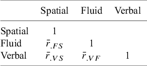
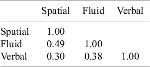


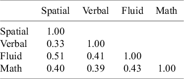
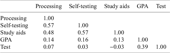
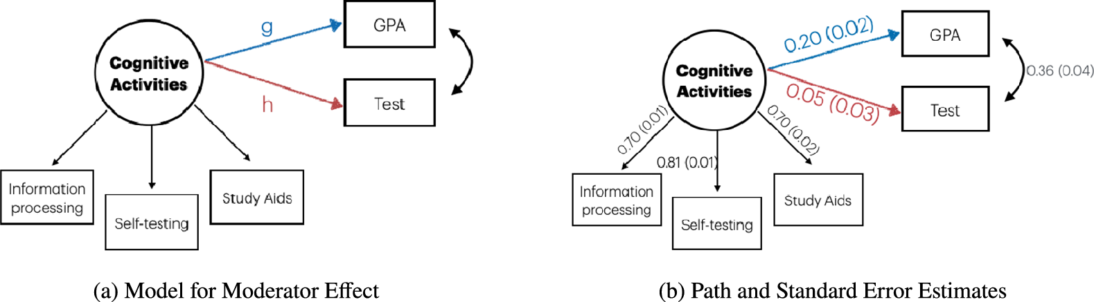

 Open access

