1 Introduction
Most of the approaches to turbulence are based on a level or scale decomposition of the full turbulent field. Famous examples are the Reynolds decomposition of the flow in a mean and fluctuating part and the spectral decomposition in a hierarchy of scales of motion. The general aim is to provide a description of turbulence simpler than that given by the full Navier–Stokes equations. However, the nonlinearity of the problem challenges for a reduced description of turbulence giving rise to the well-known closure problem in statistical theories of turbulence. It consists of a coupling of the different levels and scales composing turbulence which interact themselves exchanging momentum and kinetic energy (Domaradzki et al. Reference Domaradzki, Liu, Härtel and Kleiser1994). In this context, the large eddy decomposition represents a technique to address the multiscale approach to turbulence (Germano Reference Germano1992; Kerr, Domaradzki & Barbier Reference Kerr, Domaradzki and Barbier1996). Based on a hierarchy of filter lengths, the large eddy decomposition is probably the simplest way to give an intuitive idea of scales of motion (Borue & Orszag Reference Borue and Orszag1998) and the so-called filter-space technique (Ni, Voth & Ouellette Reference Ni, Voth and Ouellette2014), based on the removal of some degrees of freedom by filtering, represents an alternative approach to more sophisticated techniques. The main quantity in the filtering analysis of turbulent flows is the so-called subgrid turbulent stress. As remarked by Eyink (Reference Eyink2006), the subgrid stresses reflect the interactions of large-scale with small-scale velocity modes and, as such, the study of such stresses is of overwhelming interest. Hence, the subgrid stresses represent the large- and small-scale contribution to the momentum flux. Analogously, the so-called subgrid dissipation represents the energy exchange between large and small scales. A relevant example is the use of the filtering approach as an efficient quantitative method for assessing the physical multiscale phenomena at the basis of the direct and inverse cascade in turbulence (Rivera, Daniel, Chen & Ecke Reference Rivera, Daniel, Chen and Ecke2003; Chen et al. Reference Chen, Ecke, Eyink, Rivera, Wan and Xiao2006; Wang et al. Reference Wang, Wan, Chen and Chen2018). Furthermore, as shown in Germano (Reference Germano2012), the subgrid stresses formally extend to a generic large-scale filtering operator the statistical central moments and, hence, can be read as generalized central moments of the second order.
Different formulations and decompositions of the subgrid turbulent stress can be introduced, and a particular formulation based on the spatial velocity increments has been recently proposed in Germano (Reference Germano2007). This formulation suggests that the scaling properties of the mean subgrid stress are similar to the properties of the second-order structure function. Moreover, as remarked in Cimarelli & De Angelis (Reference Cimarelli and De Angelis2012), another possible merit of this formulation is to mimic the nonlinear anisotropic feature of the energy sourcing in wall flows. However, a general theory on the subgrid stresses is at present missing even if that would be very important in order to understand the scale interactions in turbulence and to face the closure problem.
The above reasonings give impetus to fundamental investigations of nonlinear interactions in turbulent flows, which may eventually provide better models. Here, we attempt to address this problem by developing alternative formalisms and closures for a reduced description of the scale-space properties of momentum and energy transfer in turbulence. The paper is organized as follows. In § 2 we theoretically exploit the properties of the subgrid stress tensor, and by starting from an alternative decomposition we derive a new formalism for their reduced description which is based on a tensorial viscosity. A generalization of the gradient model approximation is also provided. In §§ 4 and 5, we analyse both the different contributions to the subgrid stress and subgrid dissipation and the new formalism, respectively, by using direct numerical simulation (DNS) data of a turbulent channel which are in turn described in § 3. Starting from the tensorial viscosity approximation, we show in § 6 how it is possible to derive a new closure for the turbulent stresses. A preliminary assessment of the model properties together with the derivation of a tensorial dynamic procedure for the evolution of the model constants is presented in § 7. The paper is finally closed by final comments and remarks in § 8. The present results are also extended to the subgrid flux associated with a scalar field, as reported in appendix A.
In what follows we will often make use of classical nomenclature taking origin from large eddy simulation (LES) studies. However, let us remark that the developed theoretical framework allows also for the study of the momentum and energy transfer in turbulence. In this context, the filter length has to be understood as cross-over scale for the filtering technique that allows us to decompose turbulence in large and small scales. Accordingly, the subgrid stresses and subgrid dissipation are intended as observables for the study of the scale-dependent properties of the momentum flux and of the energy transfer between large and small scales, respectively.
2 Theoretical framework
Let us consider the subgrid stress tensor
 $\unicode[STIX]{x1D70F}(u_{i},u_{j})$
, defined as
 $$\begin{eqnarray}\unicode[STIX]{x1D70F}(u_{i},u_{j})=\overline{u_{i}u_{j}}-\bar{u}_{i}\bar{u}_{j},\end{eqnarray}$$
and let us assume that the generic average can be represented as (Leonard Reference Leonard1974)
 $$\begin{eqnarray}\bar{u}_{i}=\int G(\boldsymbol{x},\unicode[STIX]{x1D743})u_{i}(\unicode[STIX]{x1D743})\,\text{d}\unicode[STIX]{x1D743},\end{eqnarray}$$
where
 $$\begin{eqnarray}\int G(\boldsymbol{x},\unicode[STIX]{x1D743})\,\text{d}\unicode[STIX]{x1D743}=1\end{eqnarray}$$
and
 $G$
is the kernel of a generic filter in space. As shown in Germano (Reference Germano2007), we remark that the subgrid stresses are equivalently given by the relation
 $$\begin{eqnarray}\unicode[STIX]{x1D70F}(u_{i},u_{j})=\frac{1}{2}\iint \!G(\boldsymbol{x},\unicode[STIX]{x1D743})G(\boldsymbol{x},\unicode[STIX]{x1D6C8})[u_{i}(\unicode[STIX]{x1D743})-u_{i}(\unicode[STIX]{x1D6C8})][u_{j}(\unicode[STIX]{x1D743})-u_{j}(\unicode[STIX]{x1D6C8})]\,\text{d}\unicode[STIX]{x1D743}\,\text{d}\unicode[STIX]{x1D6C8}.\end{eqnarray}$$
Equation (2.4) directly connects the subgrid stresses with the velocity increments between two points
 $$\begin{eqnarray}\unicode[STIX]{x1D6FF}u_{i}=u_{i}(\unicode[STIX]{x1D743})-u_{i}(\unicode[STIX]{x1D6C8})\end{eqnarray}$$
in terms of a double convolution integral. As is well known, the velocity increment vector characterizes the local structure of turbulence and its study is fundamental for the characterization of the subgrid stress intermittency and energy dissipation (Cerutti & Meneveau Reference Cerutti and Meneveau1998). By introducing the fluctuations defined as
 $$\begin{eqnarray}u_{i}=\bar{u}_{i}+\unicode[STIX]{x1D710}_{i},\end{eqnarray}$$
we can decompose the subgrid stresses as
 $$\begin{eqnarray}\unicode[STIX]{x1D70F}(u_{i},u_{j})=\unicode[STIX]{x1D70F}(\bar{u}_{i},\bar{u}_{j})+\unicode[STIX]{x1D70F}(\bar{u}_{i},\unicode[STIX]{x1D710}_{j})+\unicode[STIX]{x1D70F}(\unicode[STIX]{x1D710}_{i},\bar{u}_{j})+\unicode[STIX]{x1D70F}(\unicode[STIX]{x1D710}_{i},\unicode[STIX]{x1D710}_{j}),\end{eqnarray}$$
where
 $$\begin{eqnarray}\displaystyle & \displaystyle \unicode[STIX]{x1D70F}(\bar{u}_{i},\bar{u}_{j})=\frac{1}{2}\iint \!G(\boldsymbol{x},\unicode[STIX]{x1D743})G(\boldsymbol{x},\unicode[STIX]{x1D6C8})[\bar{u}_{i}(\unicode[STIX]{x1D743})-\bar{u}_{i}(\unicode[STIX]{x1D6C8})][\bar{u}_{j}(\unicode[STIX]{x1D743})-\bar{u}_{j}(\unicode[STIX]{x1D6C8})]\,\text{d}\unicode[STIX]{x1D743}\,\text{d}\unicode[STIX]{x1D6C8}, & \displaystyle\end{eqnarray}$$
 $$\begin{eqnarray}\displaystyle & \displaystyle \unicode[STIX]{x1D70F}(\bar{u}_{i},\unicode[STIX]{x1D710}_{j})=\frac{1}{2}\iint \!G(\boldsymbol{x},\unicode[STIX]{x1D743})G(\boldsymbol{x},\unicode[STIX]{x1D6C8})[\bar{u}_{i}(\unicode[STIX]{x1D743})-\bar{u}_{i}(\unicode[STIX]{x1D6C8})][\unicode[STIX]{x1D710}_{j}(\unicode[STIX]{x1D743})-\unicode[STIX]{x1D710}_{j}(\unicode[STIX]{x1D6C8})]\,\text{d}\unicode[STIX]{x1D743}\,\text{d}\unicode[STIX]{x1D6C8}, & \displaystyle\end{eqnarray}$$
 $$\begin{eqnarray}\displaystyle & \displaystyle \unicode[STIX]{x1D70F}(\unicode[STIX]{x1D710}_{i},\unicode[STIX]{x1D710}_{j})=\frac{1}{2}\iint \!G(\boldsymbol{x},\unicode[STIX]{x1D743})G(\boldsymbol{x},\unicode[STIX]{x1D6C8})[\unicode[STIX]{x1D710}_{i}(\unicode[STIX]{x1D743})-\unicode[STIX]{x1D710}_{i}(\unicode[STIX]{x1D6C8})][\unicode[STIX]{x1D710}_{j}(\unicode[STIX]{x1D743})-\unicode[STIX]{x1D710}_{j}(\unicode[STIX]{x1D6C8})]\,\text{d}\unicode[STIX]{x1D743}\,\text{d}\unicode[STIX]{x1D6C8}. & \displaystyle\end{eqnarray}$$
We remark that this decomposition is Galilean invariant, due to the fact that it is composed of Galilean invariant terms. The decomposition of subgrid stresses is recognized to be a fundamental step for the characterization and modelling of the scale-dependent properties of the momentum exchange. Indeed, from decomposition (2.7) it is possible to derive several reduced descriptions and modelling approaches. As an example, if we make the following approximation:
 $$\begin{eqnarray}\unicode[STIX]{x1D70F}(u_{i},u_{j})\approx \unicode[STIX]{x1D70F}(\bar{u}_{i},\bar{u}_{j}),\end{eqnarray}$$
we directly recover the modelling approach given by the similarity models (Bardina, Ferziger & Reynolds Reference Bardina, Ferziger and Reynolds1983b ), i.e.
 $$\begin{eqnarray}\unicode[STIX]{x1D70F}(u_{i},u_{j})\approx \unicode[STIX]{x1D70F}(\bar{u}_{i},\bar{u}_{j})=\overline{\bar{u}_{i}\bar{u}_{j}}-\bar{\bar{u}}_{i}\bar{\bar{u}}_{j}.\end{eqnarray}$$
If we also assume that the large-scale motion
 $\bar{u}_{i}$
is sufficiently smooth at the filter scale, by considering in (2.8) the following expansion:
 $$\begin{eqnarray}\left.\begin{array}{@{}c@{}}\bar{u}_{i}(\unicode[STIX]{x1D743})-\bar{u}_{i}(\unicode[STIX]{x1D6C8})\approx (\unicode[STIX]{x1D709}_{k}-\unicode[STIX]{x1D702}_{k})\unicode[STIX]{x2202}_{k}\bar{u}_{i}\\ \bar{u}_{j}(\unicode[STIX]{x1D743})-\bar{u}_{j}(\unicode[STIX]{x1D6C8})\approx (\unicode[STIX]{x1D709}_{h}-\unicode[STIX]{x1D702}_{h})\unicode[STIX]{x2202}_{h}\bar{u}_{j}\end{array}\right\}\end{eqnarray}$$
we obtain a generalized form of the so-called gradient model approximation for the subgrid stresses (Clark, Ferziger & Reynolds Reference Clark, Ferziger and Reynolds1979):
 $$\begin{eqnarray}\unicode[STIX]{x1D70F}(u_{i},u_{j})\approx \unicode[STIX]{x1D70F}(\bar{u}_{i},\bar{u}_{j})\approx -\unicode[STIX]{x1D708}_{kj}^{(g)}\unicode[STIX]{x2202}_{k}\bar{u}_{i}-\unicode[STIX]{x1D708}_{ki}^{(g)}\unicode[STIX]{x2202}_{k}\bar{u}_{j},\end{eqnarray}$$
where the associated subgrid viscosity is a tensor given by
 $$\begin{eqnarray}\unicode[STIX]{x1D708}_{ki}^{(g)}=-{\textstyle \frac{1}{2}}\unicode[STIX]{x1D70F}(x_{k},x_{h})\unicode[STIX]{x2202}_{h}\bar{u}_{i}\end{eqnarray}$$
and
 $$\begin{eqnarray}\unicode[STIX]{x1D70F}(x_{k},x_{h})=\frac{1}{2}\iint \!G(\boldsymbol{x},\unicode[STIX]{x1D743})G(\boldsymbol{x},\unicode[STIX]{x1D6C8})(\unicode[STIX]{x1D709}_{k}-\unicode[STIX]{x1D702}_{k})(\unicode[STIX]{x1D709}_{h}-\unicode[STIX]{x1D702}_{h})\,\text{d}\unicode[STIX]{x1D743}\,\text{d}\unicode[STIX]{x1D6C8}.\end{eqnarray}$$
When considering a regular Cartesian control volume and a top-hat filter, we have
 $$\begin{eqnarray}\unicode[STIX]{x1D70F}(x_{k},x_{h})={\textstyle \frac{1}{12}}\unicode[STIX]{x1D6E5}_{h}^{2}\unicode[STIX]{x1D6FF}_{kh},\end{eqnarray}$$
where
 $\unicode[STIX]{x1D6E5}_{h}$
are the lengths of the filtering operation in the three spatial directions. In these settings, the generalized gradient model (2.14) recovers the classical approximation
 $$\begin{eqnarray}\unicode[STIX]{x1D70F}(u_{i},u_{j})\approx \unicode[STIX]{x1D70F}(\bar{u}_{i},\bar{u}_{j})\approx {\textstyle \frac{1}{12}}\unicode[STIX]{x1D6E5}_{h}^{2}\unicode[STIX]{x2202}_{h}\bar{u}_{i}\unicode[STIX]{x2202}_{h}\bar{u}_{j}.\end{eqnarray}$$
Hence, in a LES context, the generalized gradient model approximation (2.14) can be understood as a refinement of the classical gradient model (2.18) in complex flows where unstructured irregular grids are commonly employed.
Accordingly with the above examples, the study of the subgrid stress decomposition (2.7) is recognized to highlight the complex nature of the small-scale motion and to reveal different modelling approaches. In this respect, we remark however that another possible decomposition of the subgrid stresses can be used in order to further shed light on the small-scale motion and its modelling. This decomposition is given by
 $$\begin{eqnarray}\unicode[STIX]{x1D70F}(u_{i},u_{j})=[\unicode[STIX]{x1D70F}(\bar{u}_{i},u_{j})+\unicode[STIX]{x1D70F}(\unicode[STIX]{x1D710}_{i},u_{j})+\unicode[STIX]{x1D70F}(u_{i},\bar{u}_{j})+\unicode[STIX]{x1D70F}(u_{i},\unicode[STIX]{x1D710}_{j})]/\,2,\end{eqnarray}$$
where
 $$\begin{eqnarray}\unicode[STIX]{x1D70F}(\bar{u}_{i},u_{j})=\frac{1}{2}\iint \!G(\boldsymbol{x},\unicode[STIX]{x1D743})G(\boldsymbol{x},\unicode[STIX]{x1D6C8})[\bar{u}_{i}(\unicode[STIX]{x1D743})-\bar{u}_{i}(\unicode[STIX]{x1D6C8})][u_{j}(\unicode[STIX]{x1D743})-u_{j}(\unicode[STIX]{x1D6C8})]\,\text{d}\unicode[STIX]{x1D743}\,\text{d}\unicode[STIX]{x1D6C8}\end{eqnarray}$$
and
 $$\begin{eqnarray}\unicode[STIX]{x1D70F}(\unicode[STIX]{x1D710}_{i},u_{j})=\frac{1}{2}\iint \!G(\boldsymbol{x},\unicode[STIX]{x1D743})G(\boldsymbol{x},\unicode[STIX]{x1D6C8})[\unicode[STIX]{x1D710}_{i}(\unicode[STIX]{x1D743})-\unicode[STIX]{x1D710}_{i}(\unicode[STIX]{x1D6C8})][u_{j}(\unicode[STIX]{x1D743})-u_{j}(\unicode[STIX]{x1D6C8})]\,\text{d}\unicode[STIX]{x1D743}\,\text{d}\unicode[STIX]{x1D6C8}.\end{eqnarray}$$
We remark that also this decomposition of the subgrid stresses is Galilean invariant as clearly highlighted by the Galilean invariance of different terms. Moreover let us notice that the tie between the two decompositions is given by the following relations:
 $$\begin{eqnarray}\displaystyle & \displaystyle [\unicode[STIX]{x1D70F}(\bar{u}_{i},u_{j})+\unicode[STIX]{x1D70F}(u_{i},\bar{u}_{j})]/2=\unicode[STIX]{x1D70F}(\bar{u}_{i},\bar{u}_{j})+[\unicode[STIX]{x1D70F}(\bar{u}_{i},\unicode[STIX]{x1D710}_{j})+\unicode[STIX]{x1D70F}(\unicode[STIX]{x1D710}_{i},\bar{u}_{j})]/2, & \displaystyle\end{eqnarray}$$
 $$\begin{eqnarray}\displaystyle & \displaystyle [\unicode[STIX]{x1D70F}(\unicode[STIX]{x1D710}_{i},u_{j})+\unicode[STIX]{x1D70F}(u_{i},\unicode[STIX]{x1D710}_{j})]/2=\unicode[STIX]{x1D70F}(\unicode[STIX]{x1D710}_{i},\unicode[STIX]{x1D710}_{j})+[\unicode[STIX]{x1D70F}(\bar{u}_{i},\unicode[STIX]{x1D710}_{j})+\unicode[STIX]{x1D70F}(\unicode[STIX]{x1D710}_{i},\bar{u}_{j})]/2. & \displaystyle\end{eqnarray}$$
Starting from the decomposition (2.19), a different approximation for the subgrid stresses could be the following:
 $$\begin{eqnarray}\unicode[STIX]{x1D70F}(u_{i},u_{j})\approx [\unicode[STIX]{x1D70F}(\bar{u}_{i},u_{j})+\unicode[STIX]{x1D70F}(u_{i},\bar{u}_{j})]/2,\end{eqnarray}$$
which, coupled with the expansions (2.13), would lead to a different approach to the subgrid stresses in the form
 $$\begin{eqnarray}\unicode[STIX]{x1D70F}(u_{i},u_{j})\approx -\unicode[STIX]{x1D708}_{kj}\unicode[STIX]{x2202}_{k}\bar{u}_{i}-\unicode[STIX]{x1D708}_{ki}\unicode[STIX]{x2202}_{k}\bar{u}_{j},\end{eqnarray}$$
where the associated subgrid viscosity is a tensor given by
 $$\begin{eqnarray}\unicode[STIX]{x1D708}_{ki}=-\frac{1}{2}\unicode[STIX]{x1D70F}(x_{k},u_{i})=-\frac{1}{4}\iint \!G(\boldsymbol{x},\unicode[STIX]{x1D743})G(\boldsymbol{x},\unicode[STIX]{x1D6C8})[\unicode[STIX]{x1D709}_{k}-\unicode[STIX]{x1D702}_{k}][u_{i}(\unicode[STIX]{x1D743})-u_{i}(\unicode[STIX]{x1D6C8})]\,\text{d}\unicode[STIX]{x1D743}\,\text{d}\unicode[STIX]{x1D6C8}.\end{eqnarray}$$
Let us point out that in the proposed subgrid stress approximation (2.25) and the related subgrid viscosity (2.26), there is no proportionality between the turbulent stress tensor and the strain rate tensor, thus removing the limitation related to classical eddy viscosity models. Indeed, it is well known that the alignment of the subgrid flux tensor with the strain rate is not verified (Härtel et al. Reference Härtel, Kleiser, Unger and Friedrich1994), also in isotropic homogeneous turbulence (Abbà, Cercignani & Valdettaro Reference Abbà, Cercignani and Valdettaro2003).
In closing this section, let us point out that the same reasoning here reported for the derivation of tensorial subgrid viscosity approach for the subgrid stresses can be easily extended also for the subgrid flux associated with a scalar field as reported in appendix A. Moreover, we stress that the present analysis has been conducted for a generic filtering operation. If the filtering operator is the Reynolds average, provided by the usual properties of the statistical average, it is easy to show that the classical decomposition (2.7) leads to
 $$\begin{eqnarray}\unicode[STIX]{x1D70F}(u_{i},u_{j})=\unicode[STIX]{x1D70F}(\unicode[STIX]{x1D710}_{i},\unicode[STIX]{x1D710}_{j})=\overline{\unicode[STIX]{x1D710}_{i}\unicode[STIX]{x1D710}_{j}}\end{eqnarray}$$
since
 $\unicode[STIX]{x1D70F}(\bar{u}_{i},\bar{u}_{j})=0$
and
 $\unicode[STIX]{x1D70F}(\bar{u}_{i},\unicode[STIX]{x1D710}_{j})+\unicode[STIX]{x1D70F}(\unicode[STIX]{x1D710}_{i},\bar{u}_{j})=0$
. Analogously, the alternative decomposition (2.19) leads to
 $$\begin{eqnarray}\unicode[STIX]{x1D70F}(u_{i},u_{j})=[\unicode[STIX]{x1D70F}(\unicode[STIX]{x1D710}_{i},u_{j})+\unicode[STIX]{x1D70F}(u_{i},\unicode[STIX]{x1D710}_{j})]/2=\overline{\unicode[STIX]{x1D710}_{i}\unicode[STIX]{x1D710}_{j}}\end{eqnarray}$$
since
 $[\unicode[STIX]{x1D70F}(\bar{u}_{i},u_{j})+\unicode[STIX]{x1D70F}(u_{i},\bar{u}_{j})]/2=0$
. The right-hand sides of (2.27) and (2.28) are then recognized as the Reynolds stresses.
3 Filtered DNS data set
In order to study the properties of the different decompositions of the subgrid stresses defined in (2.7) and (2.19) and of the tensorial subgrid viscosity defined in (2.26), we use DNS data of a turbulent channel. Indeed, due to its statistical symmetries, the turbulent channel represents the simplest kind of inhomogeneous and anisotropic flow, thus allowing for detailed statistical analysis of the physical mechanisms underlying turbulence.
The DNS data are obtained by means of a pseudo-spectral simulation of a turbulent channel at a nominal friction Reynolds number
 $Re_{\unicode[STIX]{x1D70F}}=550$
. The width of the numerical domain is
 $({\mathcal{D}}_{x},{\mathcal{D}}_{y},{\mathcal{D}}_{z})=(4\unicode[STIX]{x03C0}h,2h,2\unicode[STIX]{x03C0}h)$
in the streamwise, wall-normal and spanwise directions, respectively, and
 $h$
is the channel half-height. In the following the index
 $i=1,2,3$
corresponds to the
 $x,y,z$
directions, respectively. The number of Fourier modes and Chebyshev polynomials used in the horizontal and vertical directions are
 $(N_{x},N_{y},N_{z})=(768,257,768)$
which leads to a resolution
 $(\unicode[STIX]{x1D6E5}_{x}^{+},\unicode[STIX]{x1D6E5}_{y}^{+min},\unicode[STIX]{x1D6E5}_{y}^{+max},\unicode[STIX]{x1D6E5}_{z}^{+})=(9,0.04,6.5,4.5)$
, where the superscript + denotes the customary non-dimensionalization with viscous units. The time integration is performed with a partially implicit Crank–Nicholson/Runge–Kutta scheme.
The filtered velocity field is computed by means of a top-hat filter in physical space:
 $$\begin{eqnarray}G(\boldsymbol{x},\unicode[STIX]{x1D743})=G(y,\boldsymbol{r})=\frac{1}{\unicode[STIX]{x1D6E5}_{x}\unicode[STIX]{x1D6E5}_{y}(y)\unicode[STIX]{x1D6E5}_{z}}\mathop{\prod }_{i=1}^{3}H(\unicode[STIX]{x1D6E5}_{i}^{g}/2-|r_{i}|),\end{eqnarray}$$
where
 $r_{i}=x_{i}-\unicode[STIX]{x1D709}_{i}$
,
 $\unicode[STIX]{x1D6E5}_{x}^{g}=\unicode[STIX]{x1D6E5}_{x}$
,
 $\unicode[STIX]{x1D6E5}_{z}^{g}=\unicode[STIX]{x1D6E5}_{z}$
and
 $\unicode[STIX]{x1D6E5}_{y}^{g}=2[H(r_{y})\unicode[STIX]{x1D6E5}_{y}^{t}+H(-r_{y})\unicode[STIX]{x1D6E5}_{y}^{b}]$
, with
 $\unicode[STIX]{x1D6E5}_{y}^{t}=y_{j+1}-y_{j}$
and
 $\unicode[STIX]{x1D6E5}_{y}^{b}=y_{j}-y_{j-1}$
, where
 $y_{j}$
is the vertical coordinate of the
 $j$
th computational point so that
 $\unicode[STIX]{x1D6E5}_{y}(y)=\unicode[STIX]{x1D6E5}_{y}^{t}+\unicode[STIX]{x1D6E5}_{y}^{b}$
. For the symmetries of the channel, the filter operator changes with the wall-normal position
 $y$
. It is worth noting that the filter operator is an independent variable that, together with the filter length, specifically defines the large and small scales of the decomposition. In the present context, the use of a top-hat filter is justified by its compact support in physical space so that the ranges of small and large scales are clearly defined in space. Indeed, we aim at assessing a general framework for the study of the different contributions to turbulence as an alternative to more classical approaches such as those given by the spectral decomposition where sharp-cutoff filters are certainly better suited. Furthermore, let us point out that the theoretical formalism here described is sufficiently general to overcome possible limitations given by the specific filtering operator. As an example, even in the extreme case of the Reynolds average as filtering operator, the developed formalism remains unaltered.
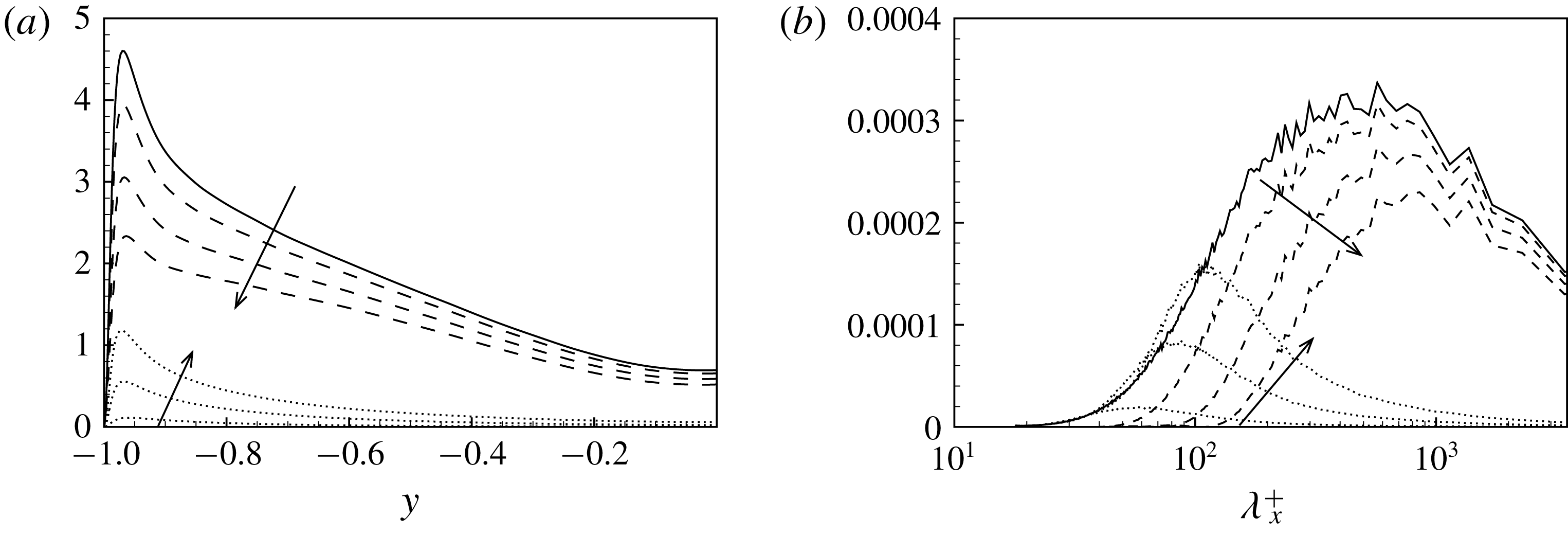
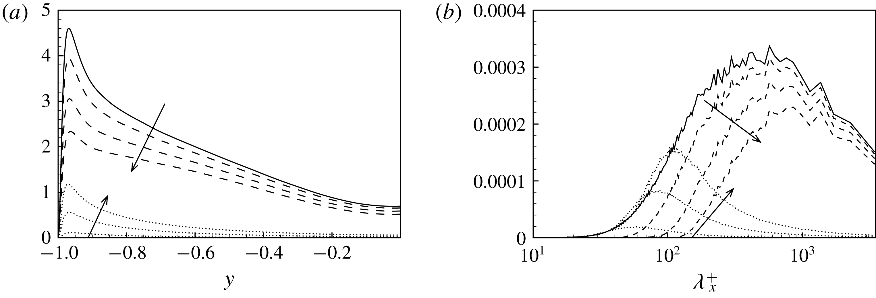
Small- and large-scale decomposition of turbulent kinetic energy given by the filtering approach. (a) The wall-normal profiles of turbulent kinetic energy associated with the large-scale,
 $\bar{u}_{i}^{+}$
, and small-scale,
 $\unicode[STIX]{x1D710}_{i}^{+}$
, motion. (b) The representation given by the premultiplied Fourier spectra of the decomposition for a single wall distance,
 $y^{+}=60$
, as a function of the streamwise wavelength. In both panels, the large- and small-scale motions are indicated with dashed and dotted lines, respectively. The arrows indicate the filtered cases F1, F2 and F3, respectively.
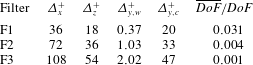
Size of the filters applied to the DNS field of turbulent channel flow. Parameters
 $\unicode[STIX]{x1D6E5}_{x}^{+}$
and
 $\unicode[STIX]{x1D6E5}_{z}^{+}$
are the filter lengths in the streamwise and spanwise directions. In the wall-normal direction the filter length varies from the smaller value at the wall
 $\unicode[STIX]{x1D6E5}_{y,w}^{+}$
to the larger one at channel centre
 $\unicode[STIX]{x1D6E5}_{y,c}^{+}$
. The ratio between the degrees of freedom of the filtered field,
 $\overline{DoF}$
, with respect those of the unfiltered one,
 $DoF$
, is also reported for the different sets of filter widths adopted.

Three sets of filter lengths have been considered and are reported in table 1. The resulting decomposition of turbulence in large- and small-scale motion is described in the left-hand panel of figure 1 where the wall-normal profiles of turbulent kinetic energy associated with the two ranges of scales are shown. In the right-hand panel of figure 1, the spectral description of the decomposition given by the filtering approach is also shown for a single relevant distance from the wall.
4 Properties of the subgrid stress decompositions
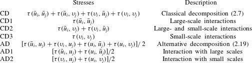
As pointed out in Germano (Reference Germano2012), the subgrid stresses and their possible decompositions can be understood as generalized central moments of the second order that are very relevant for the study of the different parts composing turbulence at different levels. For a given fixed filter length, the different parts composing turbulence are the large and small scales which nonlinearly interact among themselves and exchange momentum and energy. The study of their different decompositions could shed light on the multiscale nature of turbulence and on its modelling. The analysis will be performed by grouping together subgrid stress components of the same nature. For the sake of clarity, the expressions of the classical decompositions (2.7) and the alternative one (2.19), their components and the way they are referred to in the following analysis are reported in table 2. For reasons of brevity, we will report the statistical behaviour of the different decompositions only for the dominant component of the subgrid stress tensor, namely
 $\unicode[STIX]{x1D70F}_{12}$
.
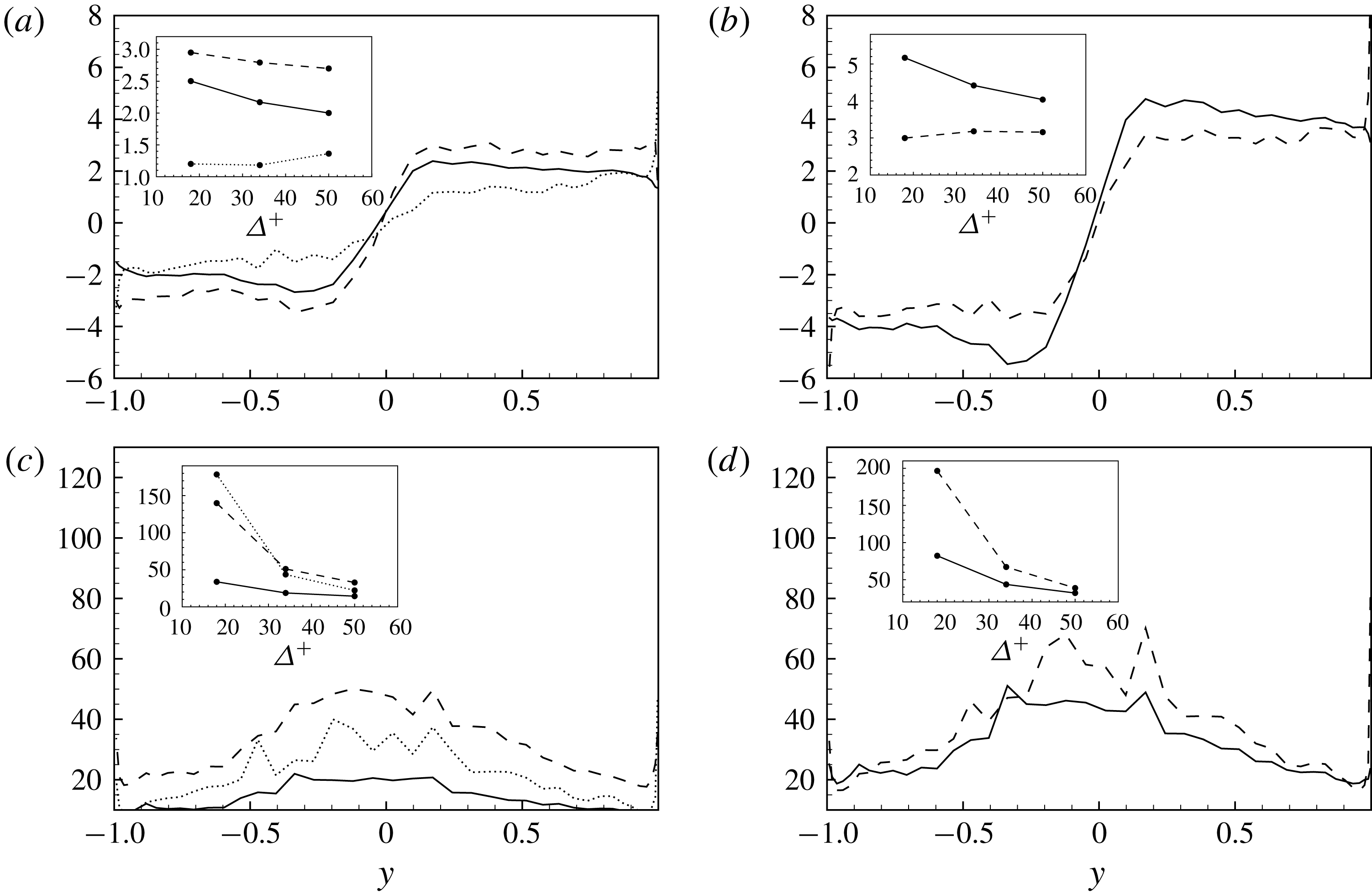
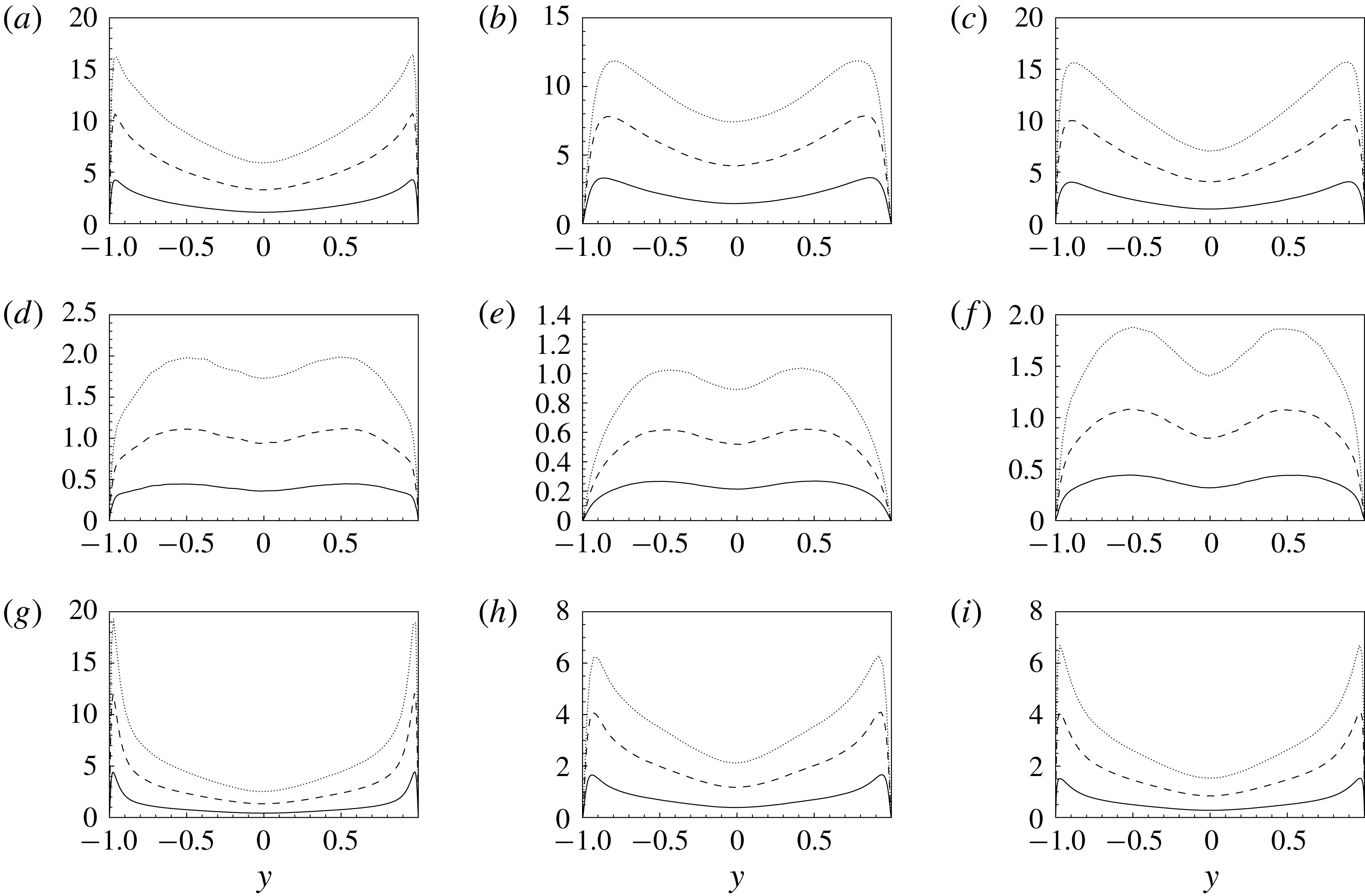
Wall-normal profiles of the mean (a,b) and variance (c,d) of the subgrid stress decomposition of
 $\unicode[STIX]{x1D70F}_{12}^{+}$
. (a,c) CD1 ——, CD2 – –, CD3
 $\cdots \,$
. (b,d) AD1 ——, AD2 – –. The profiles are shown for different filter lengths and the arrows indicate cases from F1 to F3.

Analysed stress decompositions.

In figure 2, the mean and the variance of the different decompositions of
 $\unicode[STIX]{x1D70F}_{12}$
are shown as a function of the normal to the wall coordinate for the three filter lengths considered. As expected, both the mean and variance of all the terms of the two decompositions peak in the near-wall region and decrease moving towards the channel core. The effect of filtering is to increase the intensity of the stresses. In the classical decomposition of stresses we observe that, for small filter lengths, the largest values of mean and variance are reached by the stresses associated with interactions between large scales, component CD1, while the smallest values of stresses are given by interactions between small scales, component CD3. On the other hand, by increasing the filter scale, this behaviour inverts in the near-wall region since the stresses associated with small scales, component CD3, are the most intense both in terms of mean and variance. This inversion of roles is not observed in the channel core, thus highlighting that the near-wall region is characterized by phenomena of momentum exchange where small scales play a more significant role. The stresses associated with the interactions between large and small scales, component CD2, appear to be always in between the stresses CD1 and CD3 in terms of mean and variance. The new decomposition highlights similar trends consisting, for small filter lengths, of subgrid stresses dominated by the interactions with large scales, component AD1, both in the channel core and in the near-wall region. On the other hand, for large filter scales, the subgrid stresses of the near-wall region are driven by the interactions with the small subgrid field, component AD2.
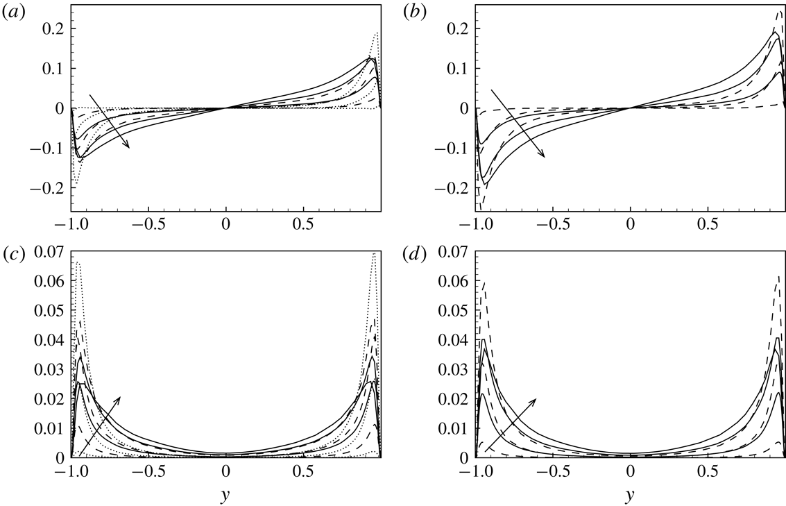
Wall-normal profiles of skewness (a,b) and kurtosis (c,d) of the subgrid stress decomposition of
 $\unicode[STIX]{x1D70F}_{12}$
. (a,c) CD1 ——, CD2 – –, CD3
 $\cdots \,$
. (b,d) AD1 ——, AD2 – –. The profiles are shown for the intermediate filter case F2. The effect of filtering is shown in the insets where the volume integral of skewness and kurtosis is shown for the three filter cases.

The wall-normal profiles of the skewness and kurtosis of the different subgrid stress decompositions are considered now in order to further characterize the properties of the decompositions. As shown in figure 3, a strong non-Gaussian behaviour is observed for all the terms composing the subgrid stresses, their distributions being significantly skewed and characterized by large levels of kurtosis. By starting from the skewness, we observe that, with the exception of a change of sign between the two halves of the channel, the profiles are almost flat. The largest values of skewness are exhibited by stresses involving the large-scale motion, i.e. components CD1, CD2 and AD1. On the other hand, the stresses associated with interactions with the small-scale field are less skewed, components CD3 and AD2. As shown in the insets of figure 3, the effect of the filter size is to decrease the levels of skewness for all the stresses with the exception of those associated with the small-scale motion, i.e. terms CD3 and AD2. With regard to kurtosis, we observe that all the profiles monotonically increase with the wall distance. Hence, the higher levels of kurtosis are reached in the channel core region. Contrarily to the behaviour of the skewness, the deviation from Gaussian behaviour is larger for the stresses CD2, CD3 and AD2 associated with the small-scale motion. Indeed, the smallest values of kurtosis are reached by stresses related to the large-scale motion, components CD1 and AD1. As shown in the insets of figure 3, also in this case, the effect of filtering is to reduce the non-Gaussian behaviour for all the terms composing the subgrid stresses. This behaviour could be related to the strongly non-Gaussian nature of the small-scale contribution to the momentum flux whose effect is weakened by the inclusion of larger and larger scales by increasing the filter length.
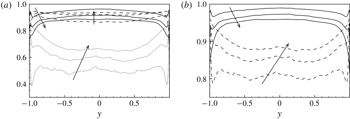
Wall-normal profiles of the correlation function
 $C_{ij}$
for the different subgrid stress decompositions of
 $\unicode[STIX]{x1D70F}_{12}$
. (a) CD1 ——, CD2 – –, CD3
 $\cdots \,$
. (b) AD1 ——, AD2 – –. The profiles are shown for different filter lengths and the arrows indicate cases from F1 to F3.

Let us now analyse the structural properties (Sagaut Reference Sagaut2001) of the decompositions of the subgrid stresses here considered, i.e. the degree to which the reduced description of the subgrid stresses given by each element of the decompositions succeeds in representing the total momentum flux. To this aim, the correlation of the different terms composing the subgrid stress decomposition
 $\unicode[STIX]{x1D70F}_{ij}^{(dec)}$
with the total ones
 $\unicode[STIX]{x1D70F}_{ij}^{(tot)}=\unicode[STIX]{x1D70F}(u_{i},u_{j})$
,
 $$\begin{eqnarray}C_{ij}(y)=\frac{\langle \unicode[STIX]{x1D70F}_{ij}^{(dec)}\unicode[STIX]{x1D70F}_{ij}^{(tot)}\rangle }{\sqrt{\langle \unicode[STIX]{x1D70F}_{ij}^{(dec)2}\rangle \langle \unicode[STIX]{x1D70F}_{ij}^{(tot)2}\rangle }},\end{eqnarray}$$
is shown in figure 4 as a function of the normal to the wall coordinate for different filter lengths. In the definition (4.1),
 $\langle \cdot \rangle$
is used to denote temporal and spatial average in the homogeneous directions. As shown in figure 4, the profiles of the contribution to the subgrid stresses of phenomena involving the large-scale motion, components CD1 and AD1, exhibit an increase of correlation with the total turbulent stresses by moving from the wall to the channel centre. On the contrary, the contributions given by the small-scale motion, components CD3 and AD2, are more correlated with the total turbulent stresses near the wall rather than in the bulk of the channel. Accordingly, with the exception of the near-wall region, the subgrid stresses CD1 and AD1 due to interactions with the large-scale motion turn out to be the best approximation of the total subgrid stresses. This result is at the basis of the well-known ability of similarity models to reproduce the structural properties of the subgrid stress tensor. This property is partially mitigated by a double effect of filtering. Indeed, a reduction of correlation with the total stresses is observed for the stresses associated with the large-scale motion, CD1 and AD1, by increasing the filter length. On the other hand, the effect of filtering is to increase the degree of correlation for the stresses due to interactions with the small-scale motion, i.e. components CD3 and AD2. This double effect of filtering is particularly effective in the near-wall region. Indeed, the contribution of stresses involving the small-scale motion, components CD3 and AD2, is found to be the best approximation of the near-wall turbulent stresses for the larger filter case F3. This aspect further supports the well-known idea of a near-wall region where the role of small scales in the phenomena of momentum flux is stronger (Domaradzki et al.
Reference Domaradzki, Liu, Härtel and Kleiser1994).
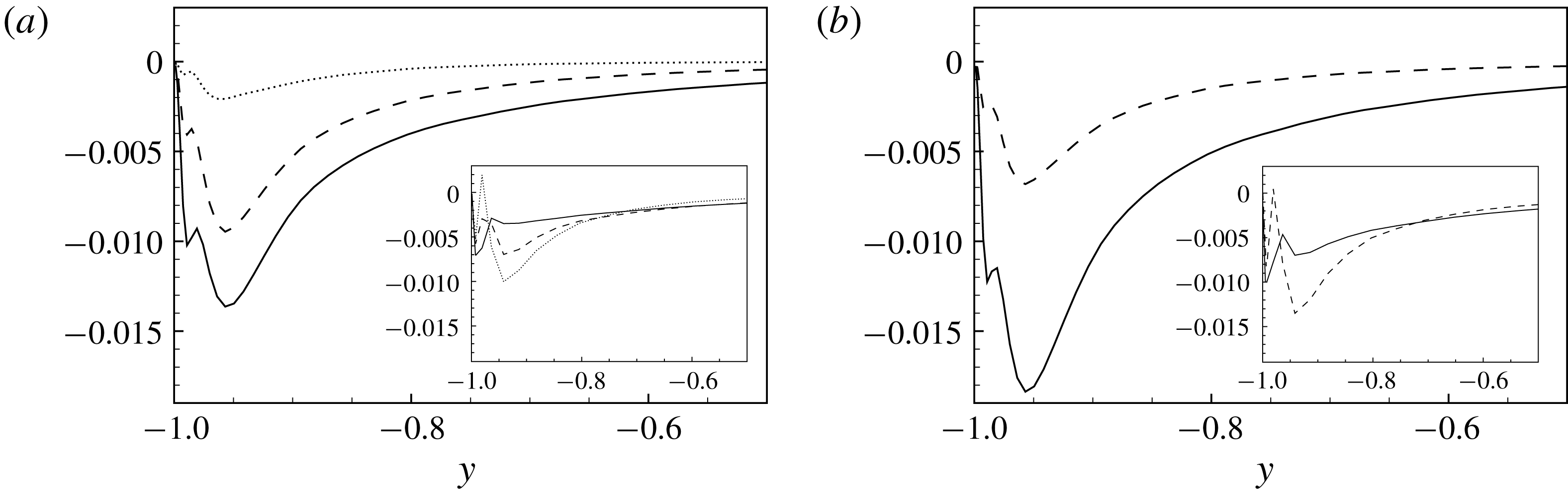
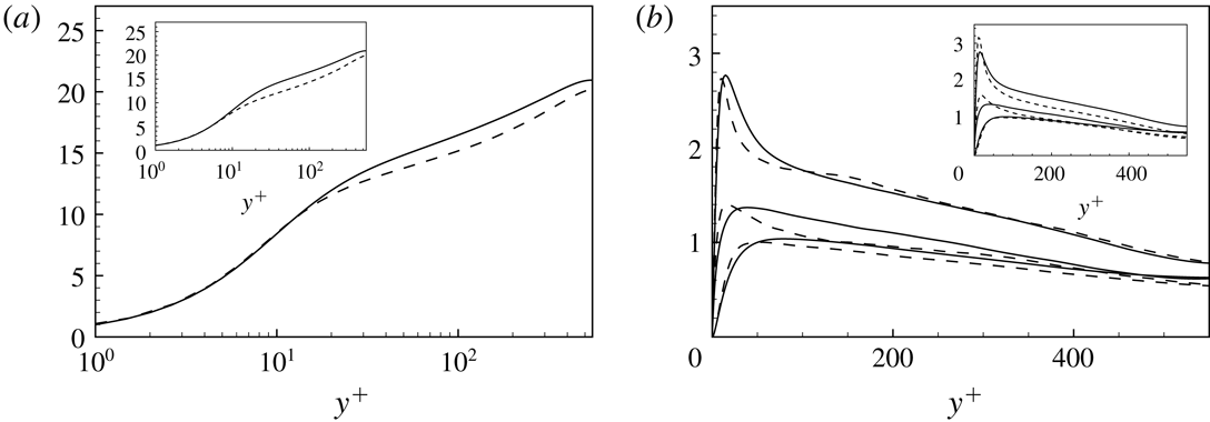
Wall-normal profiles of the subgrid dissipation
 $\unicode[STIX]{x1D716}_{sgs}^{+}$
reproduced by the different decompositions of the subgrid stresses. (a) The subgrid dissipation is computed using the components of the CD decompositions, CD1 ——, CD2 – –, CD3
 $\cdots \,$
. (b) The subgrid dissipation is computed using the components of the AD decompositions, AD1 ——, AD2 – –. In the main plots the profiles show the behaviour for the filter case F1, while in the insets for the filter case F3.

In closing this section, let us consider also the contribution of each element of the decompositions of the subgrid stresses to the overall energy transfer between large and small scales. To this aim, we study the so-called subgrid dissipation of turbulent kinetic energy defined as
 $$\begin{eqnarray}\unicode[STIX]{x1D716}_{sgs}=\langle \unicode[STIX]{x1D70F}_{ij}^{\prime }\bar{S}_{ij}^{\prime }\rangle ,\end{eqnarray}$$
where the prime denotes a fluctuating quantity and
 $\bar{S}_{ij}^{\prime }=(\unicode[STIX]{x2202}_{j}\bar{u}_{i}^{\prime }+\unicode[STIX]{x2202}_{i}\bar{u}_{j}^{\prime })/2$
is the strain rate tensor of the fluctuating resolved velocity field. In a LES context, the subgrid dissipation is recognized to represent the most important effect on the large scales of the subgrid stresses that should be reproduced accurately by models (Piomelli, Yu & Adrian Reference Piomelli, Yu and Adrian1996; Cimarelli & De Angelis Reference Cimarelli and De Angelis2014).
As shown in the main plots of figure 5, the intensity of the subgrid dissipation is higher in the near-wall region for all the terms of the decompositions and decreases moving away from the wall. This behaviour is consistent with the presence in the near-wall production region of stronger energy cascade mechanisms towards dissipation at small scales. In this context, the stresses related to interactions with large scales, components CD1 and AD1, are responsible for the larger amount of subgrid dissipation in the case of small filter lengths. Indeed, the stresses due to the interactions with the small-scale motion, CD3 and AD2, give rise to a relatively small amount of subgrid dissipation. As before, the mixed stresses CD2 of the classical decomposition show a behaviour that is always in between the two stresses associated with the large and small scales. By increasing the filter length, the contribution of stresses involving large scales to the energy transfer processes of the channel core, components CD1 and AD1, remains dominant (see the insets of figure 5). On the contrary, the behaviour of the subgrid dissipation becomes more complex in the near-wall region due to the appearance of a double peak. As also shown in Härtel et al. (Reference Härtel, Kleiser, Unger and Friedrich1994) and Cimarelli & De Angelis (Reference Cimarelli and De Angelis2012), the near-wall region for large filter lengths is characterized by a three-layer structure where two peaks of high dissipation embed a low-dissipative layer which eventually gives rise to a change of sign and, hence, to a reverse energy transfer from small to large scales,
 $\unicode[STIX]{x1D716}_{sgs}>0$
(Cimarelli, De Angelis & Casciola Reference Cimarelli, De Angelis and Casciola2013; Cimarelli et al.
Reference Cimarelli, De Angelis, Schlatter, Brethouwer, Talamelli and Casciola2015, Reference Cimarelli, De Angelis, Jiménez and Casciola2016). In this context, we observe that the contribution of stresses involving small scales in the energy transfer processes of the near-wall region becomes dominant. Indeed, as shown in the insets of figure 5, for the filter case F3, the stresses related to interactions with the small-scale motion, CD3 and AD2, are responsible for a larger amount of dissipation with respect to the stresses, CD1 and AD1, associated with the large-scale motion. In a LES context, we argue that this phenomenon is at the basis of the very low-dissipative behaviour of similarity models. It is also interesting to point out that the phenomenon of reverse energy transfer from small to large scales,
 $\unicode[STIX]{x1D716}_{sgs}>0$
, appears to be mostly reproduced by stresses given by interactions with the small-scale motion, components CD3 and AD2; for example, see the works related to this topic of Piomelli et al. (Reference Piomelli, Cabot, Moin and Lee1991) and Domaradzki et al. (Reference Domaradzki, Liu, Härtel and Kleiser1994).
As a final comment of this section, let us remark that the present analysis supports assumption (2.24), i.e.
 $$\begin{eqnarray}\unicode[STIX]{x1D70F}(u_{i},u_{j})\approx [\unicode[STIX]{x1D70F}(\bar{u}_{i},u_{j})+\unicode[STIX]{x1D70F}(u_{i},\bar{u}_{j})]/2.\end{eqnarray}$$
Indeed, for small filter lengths, the contribution of
 $[\unicode[STIX]{x1D70F}(\unicode[STIX]{x1D710}_{i},u_{j})+\unicode[STIX]{x1D70F}(u_{i},\unicode[STIX]{x1D710}_{j})]/2$
is negligible in terms of mean and fluctuating intensity (see figure 2) and in the correct reproduction of the actual stresses and of the subgrid dissipation (see figures 4 and 5). For large filter lengths, the strength of this assumption remains unaltered in the core of the channel, whereas it deteriorates close to the walls, since the contribution of
 $[\unicode[STIX]{x1D70F}(\unicode[STIX]{x1D710}_{i},u_{j})+\unicode[STIX]{x1D70F}(u_{i},\unicode[STIX]{x1D710}_{j})]/2$
overcomes that of
 $[\unicode[STIX]{x1D70F}(\bar{u}_{i},u_{j})+\unicode[STIX]{x1D70F}(u_{i},\bar{u}_{j})]/2$
. Let us point out that these results can be understood also as a measure of the scale-space locality of the momentum and energy transfer mechanisms in turbulence (Zhou Reference Zhou1993; Domaradzki, Teaca & Carati Reference Domaradzki, Teaca and Carati2009). In this context, the largest contribution given by the term AD1 with respect to AD2 to the total subgrid stresses and dissipation actually suggests that local mechanisms prevail on non-local ones in the momentum and energy transfer phenomena, respectively.
5 Properties of the tensorial subgrid viscosity
In § 2 we have shown how the general formalism of the viscosity tensor based on the velocity increments, equation (2.26), is a natural approximation for the momentum flux originating from interactions between large and small scales, equation (2.25). The degree of generality of the formalism is further supported by the fact that it can also be used to give a reduced description of the scalar flux as shown in appendix A. The main properties of the subgrid viscosity tensor are here described.
Let us point out first that the proposed subgrid viscosity (2.26) is actually strictly related to the derived generalization of the subgrid viscosity of the gradient model (2.15). Indeed, by recalling the relation (2.22)
 $$\begin{eqnarray}[\unicode[STIX]{x1D70F}(\bar{u}_{i},u_{j})+\unicode[STIX]{x1D70F}(u_{i},\bar{u}_{j})]/2=\unicode[STIX]{x1D70F}(\bar{u}_{i},\bar{u}_{j})+[\unicode[STIX]{x1D70F}(\bar{u}_{i},\unicode[STIX]{x1D710}_{j})+\unicode[STIX]{x1D70F}(\unicode[STIX]{x1D710}_{i},\bar{u}_{j})]/2,\end{eqnarray}$$
where
 $$\begin{eqnarray}\displaystyle & \displaystyle \unicode[STIX]{x1D70F}(\bar{u}_{i},u_{j})=\frac{1}{2}\iint \!G(\boldsymbol{x},\unicode[STIX]{x1D743})G(\boldsymbol{x},\unicode[STIX]{x1D6C8})[\bar{u}_{i}(\unicode[STIX]{x1D743})-\bar{u}_{i}(\unicode[STIX]{x1D6C8})][u_{j}(\unicode[STIX]{x1D743})-u_{j}(\unicode[STIX]{x1D6C8})]\,\text{d}\unicode[STIX]{x1D743}\,\text{d}\unicode[STIX]{x1D6C8}, & \displaystyle\end{eqnarray}$$
 $$\begin{eqnarray}\displaystyle & \displaystyle \unicode[STIX]{x1D70F}(\bar{u}_{i},\bar{u}_{j})=\frac{1}{2}\iint \!G(\boldsymbol{x},\unicode[STIX]{x1D743})G(\boldsymbol{x},\unicode[STIX]{x1D6C8})[\bar{u}_{i}(\unicode[STIX]{x1D743})-\bar{u}_{i}(\unicode[STIX]{x1D6C8})][\bar{u}_{j}(\unicode[STIX]{x1D743})-\bar{u}_{j}(\unicode[STIX]{x1D6C8})]\,\text{d}\unicode[STIX]{x1D743}\,\text{d}\unicode[STIX]{x1D6C8}, & \displaystyle\end{eqnarray}$$
 $$\begin{eqnarray}\displaystyle & \displaystyle \unicode[STIX]{x1D70F}(\bar{u}_{i},\unicode[STIX]{x1D710}_{j})=\frac{1}{2}\iint \!G(\boldsymbol{x},\unicode[STIX]{x1D743})G(\boldsymbol{x},\unicode[STIX]{x1D6C8})[\bar{u}_{i}(\unicode[STIX]{x1D743})-\bar{u}_{i}(\unicode[STIX]{x1D6C8})][\unicode[STIX]{x1D710}_{j}(\unicode[STIX]{x1D743})-\unicode[STIX]{x1D710}_{j}(\unicode[STIX]{x1D6C8})]\,\text{d}\unicode[STIX]{x1D743}\,\text{d}\unicode[STIX]{x1D6C8}, & \displaystyle\end{eqnarray}$$
and considering again the approximation for the filtered velocity increment (2.13), we can write
 $$\begin{eqnarray}\displaystyle & \displaystyle [\unicode[STIX]{x1D70F}(\bar{u}_{i},u_{j})+\unicode[STIX]{x1D70F}(u_{i},\bar{u}_{j})]/2\approx -\unicode[STIX]{x1D708}_{kj}\unicode[STIX]{x2202}_{k}\bar{u}_{i}-\unicode[STIX]{x1D708}_{ki}\unicode[STIX]{x2202}_{k}\bar{u}_{j}, & \displaystyle\end{eqnarray}$$
 $$\begin{eqnarray}\displaystyle & \displaystyle \unicode[STIX]{x1D70F}(\bar{u}_{i},\bar{u}_{j})\approx -\unicode[STIX]{x1D708}_{kj}^{(g)}\unicode[STIX]{x2202}_{k}\bar{u}_{i}-\unicode[STIX]{x1D708}_{ki}^{(g)}\unicode[STIX]{x2202}_{k}\bar{u}_{j}, & \displaystyle\end{eqnarray}$$
 $$\begin{eqnarray}\displaystyle & \displaystyle [\unicode[STIX]{x1D70F}(\bar{u}_{i},\unicode[STIX]{x1D710}_{j})+\unicode[STIX]{x1D70F}(\unicode[STIX]{x1D710}_{i},\bar{u}_{j})]/2\approx -\unicode[STIX]{x1D708}_{kj}^{(cross)}\unicode[STIX]{x2202}_{k}\bar{u}_{i}-\unicode[STIX]{x1D708}_{ki}^{(cross)}\unicode[STIX]{x2202}_{k}\bar{u}_{j}, & \displaystyle\end{eqnarray}$$
where the corresponding subgrid viscosities are given by
 $$\begin{eqnarray}\displaystyle & \displaystyle \unicode[STIX]{x1D708}_{ki}=-\frac{1}{4}\iint \!G(\boldsymbol{x},\unicode[STIX]{x1D743})G(\boldsymbol{x},\unicode[STIX]{x1D6C8})[\unicode[STIX]{x1D709}_{k}-\unicode[STIX]{x1D702}_{k}][u_{i}(\unicode[STIX]{x1D743})-u_{i}(\unicode[STIX]{x1D6C8})]\,\text{d}\unicode[STIX]{x1D743}\,\text{d}\unicode[STIX]{x1D6C8}, & \displaystyle\end{eqnarray}$$
 $$\begin{eqnarray}\displaystyle & \displaystyle \unicode[STIX]{x1D708}_{ki}^{(g)}=-\frac{1}{4}\unicode[STIX]{x2202}_{h}\bar{u}_{i}\iint \!G(\boldsymbol{x},\unicode[STIX]{x1D743})G(\boldsymbol{x},\unicode[STIX]{x1D6C8})(\unicode[STIX]{x1D709}_{k}-\unicode[STIX]{x1D702}_{k})(\unicode[STIX]{x1D709}_{h}-\unicode[STIX]{x1D702}_{h})\,\text{d}\unicode[STIX]{x1D743}\,\text{d}\unicode[STIX]{x1D6C8}, & \displaystyle\end{eqnarray}$$
 $$\begin{eqnarray}\displaystyle & \displaystyle \unicode[STIX]{x1D708}_{ki}^{(cross)}=-\frac{1}{4}\iint \!G(\boldsymbol{x},\unicode[STIX]{x1D743})G(\boldsymbol{x},\unicode[STIX]{x1D6C8})[\unicode[STIX]{x1D709}_{k}-\unicode[STIX]{x1D702}_{k}][\unicode[STIX]{x1D710}_{i}(\unicode[STIX]{x1D743})-\unicode[STIX]{x1D710}_{i}(\unicode[STIX]{x1D6C8})]\,\text{d}\unicode[STIX]{x1D743}\,\text{d}\unicode[STIX]{x1D6C8}. & \displaystyle\end{eqnarray}$$
By recalling now relation (5.1), we can write
 $$\begin{eqnarray}\unicode[STIX]{x1D708}_{ki}=\unicode[STIX]{x1D708}_{ki}^{(g)}+\unicode[STIX]{x1D708}_{ki}^{(cross)},\end{eqnarray}$$
thus highlighting that the present subgrid viscosity approach is composed of two contributions. The first one is given by the subgrid viscosity of the generalized gradient model
 $\unicode[STIX]{x1D708}_{ki}^{(g)}$
and, hence, is related to the stresses at large scales
 $\unicode[STIX]{x1D70F}(\bar{u}_{i},\bar{u}_{j})$
. The second one,
 $\unicode[STIX]{x1D708}_{ki}^{(cross)}$
, is due to the cross stresses
 $\unicode[STIX]{x1D70F}(\bar{u}_{i},\unicode[STIX]{x1D710}_{j})+\unicode[STIX]{x1D70F}(\unicode[STIX]{x1D710}_{i},\bar{u}_{j})$
.
Let us remark that (5.5) and (5.7) further support the idea that the subgrid viscosity tensor based on velocity increments is a natural approximation of the momentum flux arising from interactions between ranges of scales of different size. Indeed, equations (5.8) and (5.10) highlight that the same subgrid viscosity formalism allows us to represent the interactions between different types of velocity scales once the corresponding velocity increments are used, i.e.
 $u_{i}(\unicode[STIX]{x1D743})-u_{i}(\unicode[STIX]{x1D6C8})$
for the stresses
 $\unicode[STIX]{x1D70F}(\bar{u}_{i},u_{j})$
and
 $\unicode[STIX]{x1D710}_{i}(\unicode[STIX]{x1D743})-\unicode[STIX]{x1D710}_{i}(\unicode[STIX]{x1D6C8})$
for the stresses
 $\unicode[STIX]{x1D70F}(\bar{u}_{i},\unicode[STIX]{x1D710}_{j})$
.
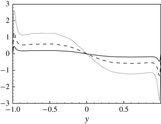
Mean wall-normal profiles of
 $\unicode[STIX]{x1D708}_{21}^{+}$
which is the only non-zero mean component of the subgrid viscosity tensor (2.26). All three sets of filter lengths are shown: F1 (solid line), F2 (dashed line) and F3 (dotted line).

Wall-normal profiles of the standard deviation of
 $\unicode[STIX]{x1D708}_{ij}^{+}$
. The
 $j$
-index goes from 1 to 3 moving from the panels on the left-hand side to the right-hand side while the
 $i$
-index goes from 1 to 3 moving from the top to the bottom panels. All three sets of filter lengths are shown: F1 (solid line), F2 (dashed line) and F3 (dotted line).

Let us now analyse the complex features unveiled by the subgrid viscosity tensor (2.26) in the turbulent channel flow. It is first worth pointing out that in homogeneous isotropic turbulence all the mean components of the subgrid viscosity tensor (2.26) are null,
 $\langle \unicode[STIX]{x1D708}_{ki}\rangle =0$
, where
 $\langle \cdot \rangle$
denotes spatial average in the homogeneous directions and temporal average. Whereas, in inhomogeneous flows we have non-zero average components. In the case of a channel flow, the only non-zero average component is
 $\unicode[STIX]{x1D708}_{21}$
. This is one of the
 $\unicode[STIX]{x1D708}_{2i}$
-components that are used in conjunction with wall-normal gradients of the velocity field for the reconstruction of the subgrid stresses (equation (2.25)). As shown in figure 6, the mean value of the subgrid viscosity peaks in the near-wall region and, as expected, is found to increase its magnitude by increasing the filter length. An antisymmetric behaviour with respect to the centreline of the channel is also observed.
The variance of the subgrid viscosity components is shown in figure 7 for different filter lengths. The overall behaviour consists of wall-normal profiles which start from zero at the wall, reach a maximum in the near-wall region and then decrease exhibiting a relative minimum in the channel centre. The effect of the filter length is to increase the intensity of the fluctuations of the subgrid viscosity for all its components. The anisotropy of the subgrid viscosity tensor is such that the most intense fluctuations are those of the
 $\unicode[STIX]{x1D708}_{1i}$
-components, i.e. those that are used in conjunction with the streamwise gradient of the velocity field to reconstruct the subgrid stress tensor (see equation (2.25)). The anisotropy of the subgrid viscosity tensor reveals itself also in the shape of the wall-normal profiles. Indeed, from figure 7 it can be seen that the profiles of the
 $\unicode[STIX]{x1D708}_{2i}$
-components show a less sharp behaviour with maxima located slightly further away from the wall with respect to the
 $\unicode[STIX]{x1D708}_{1i}$
- and
 $\unicode[STIX]{x1D708}_{3i}$
-components.
Wall-normal profiles of the third-order moment of
 $\unicode[STIX]{x1D708}_{ij}$
. The
 $j$
-index goes from 1 to 3 moving from the panels on the left-hand side to the right-hand side while the
 $i$
-index goes from 1 to 3 moving from the top to the bottom panels. All three sets of filter lengths are shown: F1 (solid line), F2 (dashed line) and F3 (dotted line).
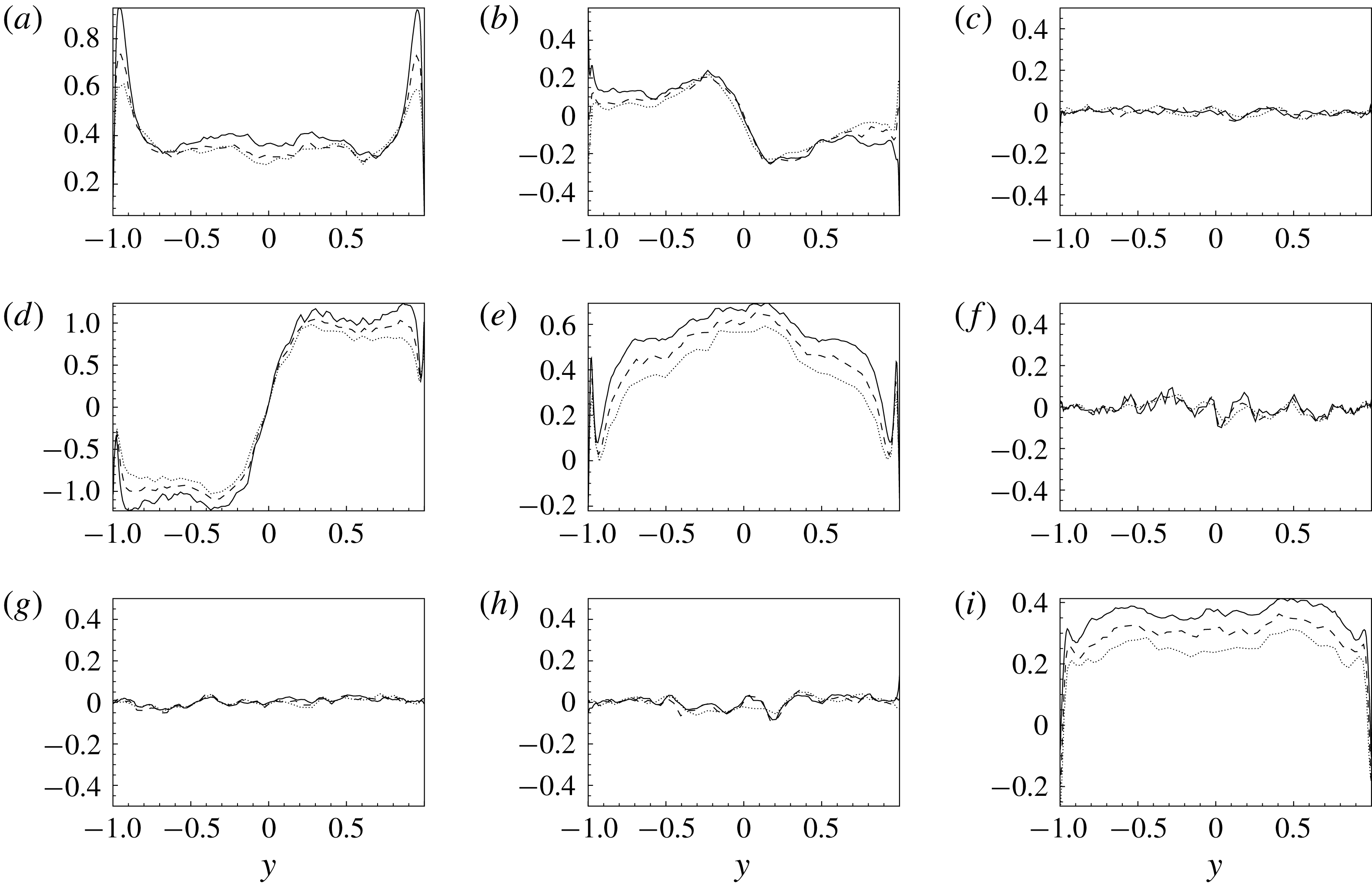
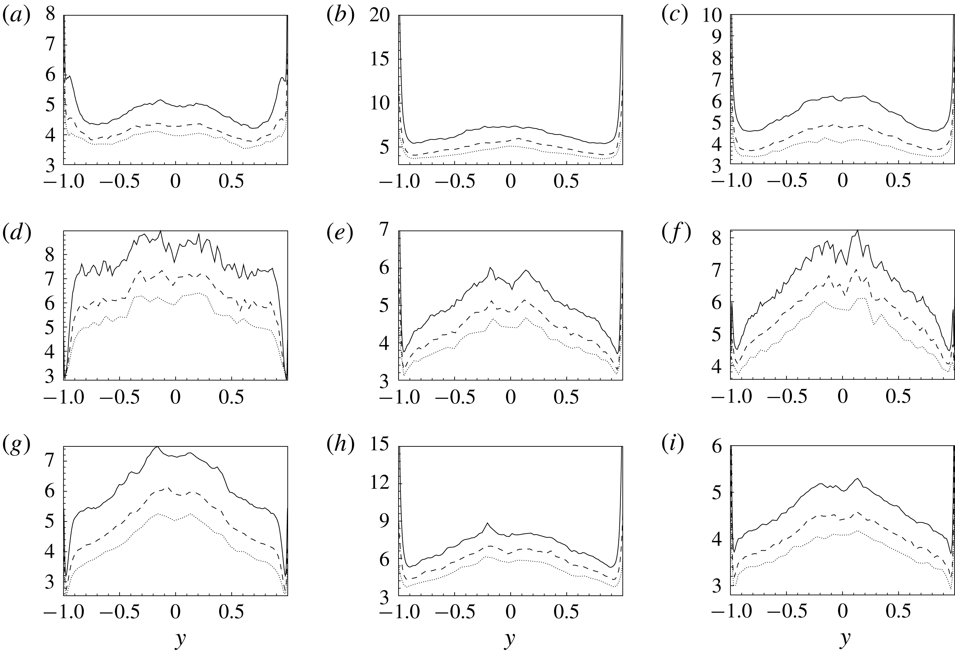
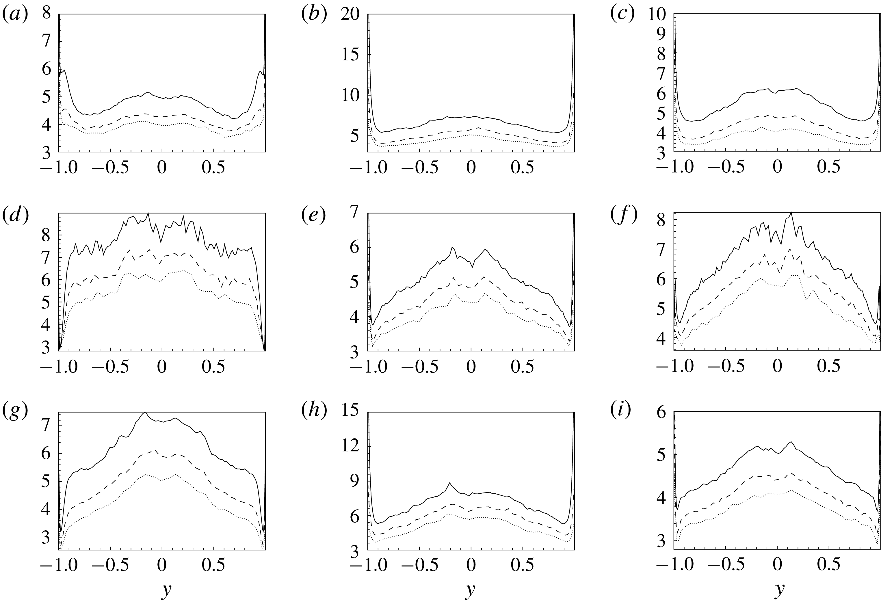
In figures 8 and 9, the third-order (skewness) and fourth-order (kurtosis) moments of the subgrid viscosity tensor (2.26), respectively
 $$\begin{eqnarray}\frac{\langle \unicode[STIX]{x1D708}_{ij}^{\prime 3}\rangle }{\langle \unicode[STIX]{x1D708}_{ij}^{\prime 2}\rangle ^{3/2}}\quad \text{and}\quad \frac{\langle \unicode[STIX]{x1D708}_{ij}^{\prime 4}\rangle }{\langle \unicode[STIX]{x1D708}_{ij}^{\prime 2}\rangle ^{2}},\end{eqnarray}$$
are shown. As shown in figure 8, the behaviour of the subgrid viscosity is significantly skewed. However, different behaviours are observed for the different components. In particular, the diagonal components,
 $\unicode[STIX]{x1D708}_{ij}$
with
 $i=j$
, exhibit a positively skewed symmetric behaviour with respect the channel centre, while the deviatoric components
 $\unicode[STIX]{x1D708}_{12}$
and
 $\unicode[STIX]{x1D708}_{21}$
are antisymmetric. The other deviatoric components,
 $\unicode[STIX]{x1D708}_{13}$
,
 $\unicode[STIX]{x1D708}_{23}$
,
 $\unicode[STIX]{x1D708}_{31}$
and
 $\unicode[STIX]{x1D708}_{32}$
, recover the normal distribution, their skewness being statistically zero. Interestingly, the effect of filtering is to reduce the non-Gaussian nature of the subgrid viscosity in accordance with the behaviour of the subgrid stresses observed in the previous section. Indeed, we observe that, by increasing the filter length from case F1 to case F3, the value of skewness significantly reduces. The behaviour of the kurtosis of the subgrid viscosity is shown in figure 9. In this case a highly non-Gaussian behaviour is observed for all the components of the subgrid viscosity since the wall-normal profiles of kurtosis are always larger than 3. A general behaviour is observed for all the components which consists of an increasing of intermittency from the wall up to the channel centre. As for the skewness, the effect of filtering is to reduce the intermittency of the subgrid viscosity.
Wall-normal profiles of the fourth-order moment of
 $\unicode[STIX]{x1D708}_{ij}$
. The
 $j$
-index goes from 1 to 3 moving from the panels on the left-hand side to the right-hand side while the
 $i$
-index goes from 1 to 3 moving from the top to the bottom panels. All three sets of filter lengths are shown: F1 (solid line), F2 (dashed line) and F3 (dotted line).
Instantaneously, both positive and negative values of
 $\unicode[STIX]{x1D708}_{ij}$
are present since
 $\langle \cdot \rangle =0$
for most of the components. This double feature shows a distinct topological behaviour that can be highlighted with the spatial correlation function
 $$\begin{eqnarray}R_{ij}(r_{x},r_{z},y)=\frac{\langle \unicode[STIX]{x1D708}_{ij}(x^{\prime },y,z^{\prime })\unicode[STIX]{x1D708}_{ij}(x^{\prime \prime },y,z^{\prime \prime })\rangle }{\langle \unicode[STIX]{x1D708}_{ij}^{2}\rangle (y)},\end{eqnarray}$$
where
 $r_{i}=x_{i}^{\prime }-x_{i}^{\prime \prime }$
, with
 $i=1$
and
 $i=3$
, is the increment of the coordinates in the homogeneous directions. Accordingly with the gross features of turbulent fluctuations in channel flows, the subgrid viscosity
 $\unicode[STIX]{x1D708}_{ij}$
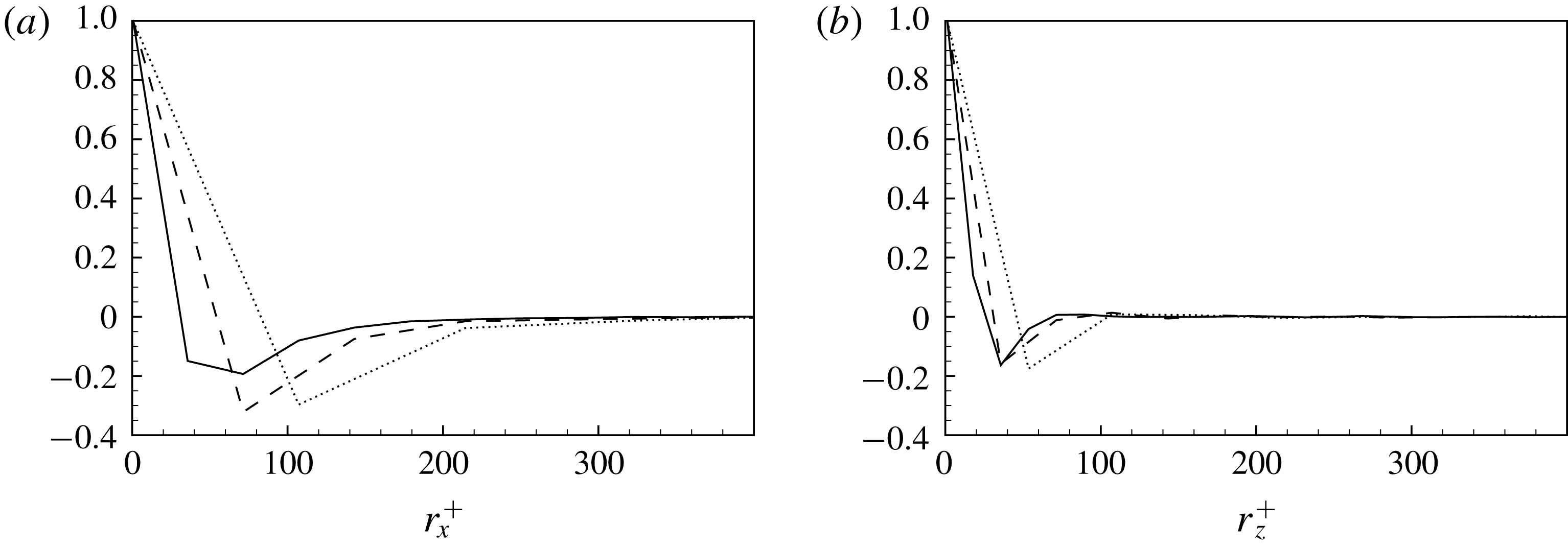
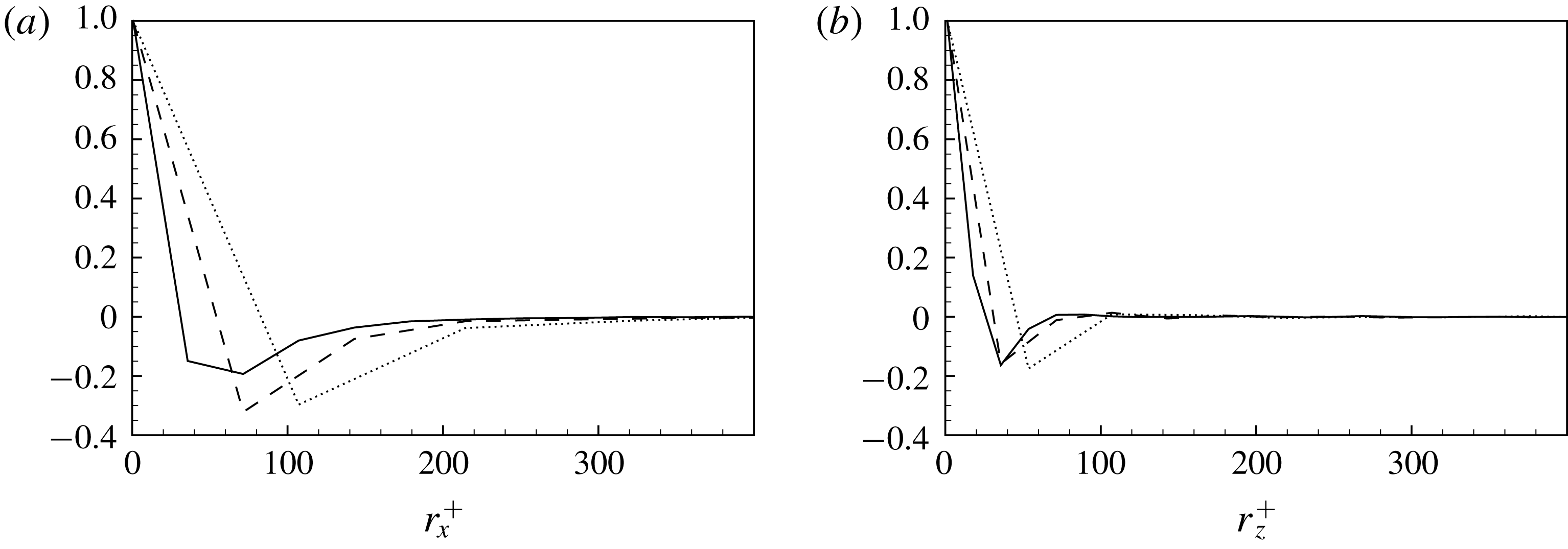
realizes a general flow pattern consisting of structures elongated in the streamwise direction. Indeed, as shown in figure 10, the spatial correlation function evaluated for a selected component of the subgrid viscosity tensor in the near-wall production region highlights a relatively short correlation length in the spanwise direction and a larger one in the streamwise direction. This topological feature is retained by all the components (not shown). Interestingly, the correlation function shows also a clear anticorrelation in both the streamwise and spanwise directions, thus highlighting that regions of positive/negative values of subgrid viscosity are statistically surrounded by regions of negative/positive values. It is worth pointing out that the approximation of the subgrid stresses given by the subgrid viscosity tensor formalism is such that negative values of
 $\unicode[STIX]{x1D708}_{ij}$
are not strictly related to phenomena of backscatter as it is for scalar subgrid viscosity approximations. Indeed, the subgrid dissipation under the subgrid viscosity tensor approximation reads
 $$\begin{eqnarray}\unicode[STIX]{x1D716}_{sgs}=-\langle (\unicode[STIX]{x1D708}_{kj}\unicode[STIX]{x2202}_{k}\bar{u}_{i}+\unicode[STIX]{x1D708}_{ki}\unicode[STIX]{x2202}_{k}\bar{u}_{j})^{\prime }\;\unicode[STIX]{x2202}_{j}\bar{u}_{i}^{\prime }\rangle ,\end{eqnarray}$$
so that backscatter can be reproduced but not necessarily with a change of sign of
 $\unicode[STIX]{x1D708}_{ij}$
.
In closing this section, let us point out that the formalism of the subgrid viscosity tensor introduced with (2.26) allows us to highlight the complexity of the small-scale motion in inhomogeneous anisotropic flows. Indeed, as shown here in quantitative terms, the subgrid viscosity tensor exhibits a strong inhomogeneous and anisotropic behaviour in terms of intensity, distribution, skewness and intermittency of its different components. Hence, it is argued how much of this complex behaviour is not taken into account by classical subgrid viscosity approaches based on more simple and restricted formalisms.
Spatial correlation coefficient
 $R_{12}$
evaluated in the near-wall production region at
 $y^{+}\approx 21$
and shown as a function of the streamwise (left) and spanwise (right) increment. All three sets of filter lengths are shown: F1 (solid line), F2 (dashed line) and F3 (dotted line).
6 Modelling approach
In this section, we show how the developed theoretical framework for the study of turbulence and, in particular, the reduced description of momentum flux given by the tensorial viscosity based on the velocity increments can be used to derive turbulence closures in a context of LES. Let us point out that the proposed modelling approaches for the subgrid viscosity can also be used for the modelling of the subgrid flux associated with a scalar field as shown in appendix A. The derivation and the main theoretical properties of the developed subgrid closures will be discussed in detail.
6.1 First-order modelling
Let us consider a top-hat filter, defined by the kernel
 $$\begin{eqnarray}G(\boldsymbol{x},\unicode[STIX]{x1D743})=\left\{\begin{array}{@{}ll@{}}1/\unicode[STIX]{x1D6FA} & \text{inside the grid element}\\ 0 & \text{otherwise},\end{array}\right.\end{eqnarray}$$
where
 $\unicode[STIX]{x1D6FA}$
is the volume of the grid element. In this case, approximation (2.26) can be rewritten as
 $$\begin{eqnarray}\unicode[STIX]{x1D708}_{ki}=-\frac{1}{4\unicode[STIX]{x1D6FA}^{2}}\int _{\unicode[STIX]{x1D6FA}}\int _{\unicode[STIX]{x1D6FA}}\!(\unicode[STIX]{x1D709}_{k}-\unicode[STIX]{x1D702}_{k})[u_{i}(\unicode[STIX]{x1D743})-u_{i}(\unicode[STIX]{x1D6C8})]\,\text{d}\unicode[STIX]{x1D743}\,\text{d}\unicode[STIX]{x1D6C8}.\end{eqnarray}$$
We now approximate the unfiltered velocity by means of an expansion of the velocity field
 $u_{i}(\unicode[STIX]{x1D743})$
around the filtered value
 $\bar{u}_{i}(\boldsymbol{x})$
,
 $$\begin{eqnarray}u_{i}(\unicode[STIX]{x1D743})=\bar{u}_{i}(\boldsymbol{x})+\unicode[STIX]{x2202}_{h}\bar{u}_{i}(\boldsymbol{x})(\unicode[STIX]{x1D709}_{h}-x_{h})+\mathit{O}^{2},\end{eqnarray}$$
where
 $\boldsymbol{x}$
is the position of the barycentre of the grid element and only the first-order derivatives are considered. By applying this approximation we have
 $$\begin{eqnarray}\displaystyle \unicode[STIX]{x1D708}_{ki} & & \displaystyle =-\frac{1}{4\unicode[STIX]{x1D6FA}^{2}}\int _{\unicode[STIX]{x1D6FA}}\int _{\unicode[STIX]{x1D6FA}}\!(\unicode[STIX]{x1D709}_{k}-\unicode[STIX]{x1D702}_{k})[\unicode[STIX]{x2202}_{h}\bar{u}_{i}(\boldsymbol{x})(\unicode[STIX]{x1D709}_{h}-x_{h})-\unicode[STIX]{x2202}_{h}\bar{u}_{i}(\boldsymbol{x})(\unicode[STIX]{x1D702}_{h}-x_{h})]\,\text{d}\unicode[STIX]{x1D743}\,\text{d}\unicode[STIX]{x1D6C8}\nonumber\\ \displaystyle & & \displaystyle =-\frac{1}{4\unicode[STIX]{x1D6FA}^{2}}\int _{\unicode[STIX]{x1D6FA}}\int _{\unicode[STIX]{x1D6FA}}\![(\unicode[STIX]{x1D709}_{k}-x_{k})-(\unicode[STIX]{x1D702}_{k}-x_{k})][\unicode[STIX]{x2202}_{h}\bar{u}_{i}(\boldsymbol{x})(\unicode[STIX]{x1D709}_{h}-x_{h})-\unicode[STIX]{x2202}_{h}\bar{u}_{i}(\boldsymbol{x})(\unicode[STIX]{x1D702}_{h}-x_{h})]\,\text{d}\unicode[STIX]{x1D743}\,\text{d}\unicode[STIX]{x1D6C8}\nonumber\\ \displaystyle & & \displaystyle =-\frac{1}{4\unicode[STIX]{x1D6FA}^{2}}\unicode[STIX]{x2202}_{h}\bar{u}_{i}(\boldsymbol{x})\int _{\unicode[STIX]{x1D6FA}}\int _{\unicode[STIX]{x1D6FA}}\![(\unicode[STIX]{x1D709}_{k}-x_{k})-(\unicode[STIX]{x1D702}_{k}-x_{k})][(\unicode[STIX]{x1D709}_{h}-x_{h})-(\unicode[STIX]{x1D702}_{h}-x_{h})]\,\text{d}\unicode[STIX]{x1D743}\,\text{d}\unicode[STIX]{x1D6C8}\nonumber\\ \displaystyle & & \displaystyle =-\frac{1}{4\unicode[STIX]{x1D6FA}^{2}}\unicode[STIX]{x2202}_{h}\bar{u}_{i}(\boldsymbol{x})\left\{\int _{\unicode[STIX]{x1D6FA}}\int _{\unicode[STIX]{x1D6FA}}\!(\unicode[STIX]{x1D709}_{k}-x_{k})(\unicode[STIX]{x1D709}_{h}-x_{h})\,\text{d}\unicode[STIX]{x1D743}\,\text{d}\unicode[STIX]{x1D6C8}+\int _{\unicode[STIX]{x1D6FA}}\int _{\unicode[STIX]{x1D6FA}}\!(\unicode[STIX]{x1D702}_{k}-x_{k})(\unicode[STIX]{x1D702}_{h}-x_{h})\,\text{d}\unicode[STIX]{x1D743}\,\text{d}\unicode[STIX]{x1D6C8}\right.\nonumber\\ \displaystyle & & \displaystyle \left.-\int _{\unicode[STIX]{x1D6FA}}\int _{\unicode[STIX]{x1D6FA}}\!(\unicode[STIX]{x1D709}_{k}-x_{k})(\unicode[STIX]{x1D702}_{h}-x_{h})\,\text{d}\unicode[STIX]{x1D743}\,\text{d}\unicode[STIX]{x1D6C8}-\int _{\unicode[STIX]{x1D6FA}}\int _{\unicode[STIX]{x1D6FA}}\!(\unicode[STIX]{x1D702}_{k}-x_{k})(\unicode[STIX]{x1D709}_{h}-x_{h})\,\text{d}\unicode[STIX]{x1D743}\,\text{d}\unicode[STIX]{x1D6C8}\right\}\end{eqnarray}$$
but
 $$\begin{eqnarray}\int _{\unicode[STIX]{x1D6FA}}\int _{\unicode[STIX]{x1D6FA}}\!(\unicode[STIX]{x1D702}_{k}-x_{k})(\unicode[STIX]{x1D709}_{h}-x_{h})\,\text{d}\unicode[STIX]{x1D743}\,\text{d}\unicode[STIX]{x1D6C8}=\int _{\unicode[STIX]{x1D6FA}}\!(\unicode[STIX]{x1D702}_{k}-x_{k})\int _{\unicode[STIX]{x1D6FA}}\!(\unicode[STIX]{x1D709}_{h}-x_{h})\,\text{d}\unicode[STIX]{x1D743}\,\text{d}\unicode[STIX]{x1D6C8}=0\end{eqnarray}$$
and, hence, the turbulent viscosity tensor takes the following form:
 $$\begin{eqnarray}\unicode[STIX]{x1D708}_{ki}=-\frac{1}{2\unicode[STIX]{x1D6FA}}\unicode[STIX]{x2202}_{h}\bar{u}_{i}(\boldsymbol{x})\int _{\unicode[STIX]{x1D6FA}}\!(\unicode[STIX]{x1D709}_{k}-x_{k})(\unicode[STIX]{x1D709}_{h}-x_{h})\,\text{d}\unicode[STIX]{x1D743}.\end{eqnarray}$$
The proposed model (6.6) for the turbulent viscosity exploits the idea of taking into account the distribution of velocity in the three spatial directions within the integration volume for filtering as suggested by the tensorial approximation (2.26). The way this idea is realized is based simply on the concept that the structure of the integration volume used to filter out the small subgrid field directly impacts the anisotropic features of the subgrid field itself and, hence, can be used to improve the prediction of the small-scale velocity field distribution given by the filtered gradient. The structure of the integration volume (grid element in the case of implicit filters) is taken into account in the present model formulation by the integral in (6.6). Indeed, for
 $k\neq h$
the integral in (6.6) is equal to the inertial product of the grid element with respect to the barycentric axis in the directions
 $k$
and
 $h$
, respectively:
 $$\begin{eqnarray}{\mathcal{I}}_{kh}=-\int _{\unicode[STIX]{x1D6FA}}\!(\unicode[STIX]{x1D709}_{k}-x_{k})(\unicode[STIX]{x1D709}_{h}-x_{h})\,\text{d}\unicode[STIX]{x1D743},\end{eqnarray}$$
while for
 $k=h$
it becomes
 $$\begin{eqnarray}{\mathcal{I}}_{kk}-\frac{1}{2}Tr({\mathcal{I}})=-\int _{\unicode[STIX]{x1D6FA}}\!(\unicode[STIX]{x1D709}_{k}-x_{k})^{2}\,\text{d}\unicode[STIX]{x1D743},\end{eqnarray}$$
where
 ${\mathcal{I}}_{kk}$
is the inertial momentum with respect to the barycentric axis in the
 $k$
direction,
 ${\mathcal{I}}_{kh}$
are the inertial products and
 ${\mathcal{I}}$
is the barycentric inertial tensor. Hence, after having defined
 $$\begin{eqnarray}{\mathcal{I}}_{kh}^{\prime }={\mathcal{I}}_{kh}-{\textstyle \frac{1}{2}}Tr({\mathcal{I}})\unicode[STIX]{x1D6FF}_{kh},\end{eqnarray}$$
we get
 $$\begin{eqnarray}\unicode[STIX]{x1D708}_{ki}=\frac{1}{2\unicode[STIX]{x1D6FA}}{\mathcal{I}}_{kh}^{\prime }\unicode[STIX]{x2202}_{h}\bar{u}_{i},\end{eqnarray}$$
thus highlighting that the anisotropy of the integration volume is directly taken into account in the present tensorial formulation of the turbulent viscosity. In conclusion, we can rewrite the subgrid stress tensor as
 $$\begin{eqnarray}\unicode[STIX]{x1D70F}(u_{i},u_{j})=-\left(\frac{1}{2\unicode[STIX]{x1D6FA}}{\mathcal{I}}_{kh}^{\prime }\unicode[STIX]{x2202}_{h}\bar{u}_{j}\right)\unicode[STIX]{x2202}_{k}\bar{u}_{i}-\left(\frac{1}{2\unicode[STIX]{x1D6FA}}{\mathcal{I}}_{kh}^{\prime }\unicode[STIX]{x2202}_{h}\bar{u}_{i}\right)\unicode[STIX]{x2202}_{k}\bar{u}_{j}.\end{eqnarray}$$
We can observe that this formulation allows us to model also the normal subgrid stress components
 $$\begin{eqnarray}\unicode[STIX]{x1D70F}(u_{i},u_{i})=-\left(\frac{1}{\unicode[STIX]{x1D6FA}}{\mathcal{I}}_{kh}^{\prime }\unicode[STIX]{x2202}_{h}\bar{u}_{i}\right)\unicode[STIX]{x2202}_{k}\bar{u}_{i},\end{eqnarray}$$
and so the subgrid turbulent kinetic energy. Since
 ${\mathcal{I}}^{\prime }$
is a semidefinite negative matrix, the reliability condition
 $\unicode[STIX]{x1D70F}(u_{i},u_{i})\geqslant 0$
is also ensured.
6.2 Second-order modelling
In the previous section, only the first-order derivatives are considered in the expansion and higher orders are neglected. In LES, where the unfiltered fields rapidly fluctuate, this approximation could introduce a considerable error (Clark et al.
Reference Clark, Ferziger and Reynolds1979; Vreman, Guerts & Kuerten Reference Vreman, Guerts and Kuerten1997). Hence, in the following a model with higher order approximation is derived. If second-order derivatives are retained in the expansion of the velocity field
 $u_{i}(\unicode[STIX]{x1D743})$
around the filtered value
 $\bar{u}_{i}(\boldsymbol{x})$
,
 $$\begin{eqnarray}u_{i}(\unicode[STIX]{x1D743})=\bar{u}_{i}(\boldsymbol{x})+\unicode[STIX]{x2202}_{h}\bar{u}_{i}(\boldsymbol{x})(\unicode[STIX]{x1D709}_{h}-x_{h})+{\textstyle \frac{1}{2}}\unicode[STIX]{x2202}_{hl}\bar{u}_{i}(\boldsymbol{x})(\unicode[STIX]{x1D709}_{h}-x_{h})(\unicode[STIX]{x1D709}_{l}-x_{l})+\mathit{O}^{3},\end{eqnarray}$$
additional terms appear in the model for the subgrid viscosity with respect to (6.10):
 $$\begin{eqnarray}\displaystyle \unicode[STIX]{x1D708}_{ki} & = & \displaystyle \frac{1}{2\unicode[STIX]{x1D6FA}}{\mathcal{I}}_{kh}^{\prime }\unicode[STIX]{x2202}_{h}\bar{u}_{i}(\boldsymbol{x})\nonumber\\ \displaystyle & & \displaystyle -\,\frac{1}{4\unicode[STIX]{x1D6FA}^{2}}\int _{\unicode[STIX]{x1D6FA}}\int _{\unicode[STIX]{x1D6FA}}\!(\unicode[STIX]{x1D709}_{k}-\unicode[STIX]{x1D702}_{k})\frac{1}{2}\unicode[STIX]{x2202}_{hl}\bar{u}_{i}(\boldsymbol{x})[(\unicode[STIX]{x1D709}_{h}-x_{h})(\unicode[STIX]{x1D709}_{l}-x_{l})-(\unicode[STIX]{x1D702}_{h}-x_{h})(\unicode[STIX]{x1D702}_{l}-x_{l})]\text{d}\unicode[STIX]{x1D743}\,\text{d}\unicode[STIX]{x1D6C8}\nonumber\\ \displaystyle & = & \displaystyle \frac{1}{2\unicode[STIX]{x1D6FA}}{\mathcal{I}}_{kh}^{\prime }\unicode[STIX]{x2202}_{h}\bar{u}_{i}(\boldsymbol{x})\nonumber\\ \displaystyle & & \displaystyle -\,\frac{1}{4\unicode[STIX]{x1D6FA}^{2}}\unicode[STIX]{x2202}_{hl}\bar{u}_{i}(\boldsymbol{x})\int _{\unicode[STIX]{x1D6FA}}\int _{\unicode[STIX]{x1D6FA}}\!\frac{1}{2}[(\unicode[STIX]{x1D709}_{k}-x_{k})(\unicode[STIX]{x1D709}_{h}-x_{h})(\unicode[STIX]{x1D709}_{l}-x_{l})+(\unicode[STIX]{x1D702}_{k}-x_{k})(\unicode[STIX]{x1D702}_{h}-x_{h})(\unicode[STIX]{x1D702}_{l}-x_{l})]\nonumber\\ \displaystyle & & \displaystyle \times \,\text{d}\unicode[STIX]{x1D743}\,\text{d}\unicode[STIX]{x1D6C8}\nonumber\\ \displaystyle & = & \displaystyle \frac{1}{2\unicode[STIX]{x1D6FA}}{\mathcal{I}}_{kh}^{\prime }\unicode[STIX]{x2202}_{h}\bar{u}_{i}(\boldsymbol{x})\nonumber\\ \displaystyle & & \displaystyle -\,\frac{1}{4\unicode[STIX]{x1D6FA}}\unicode[STIX]{x2202}_{hl}\bar{u}_{i}(\boldsymbol{x})\int _{\unicode[STIX]{x1D6FA}}\!(\unicode[STIX]{x1D709}_{k}-x_{k})(\unicode[STIX]{x1D709}_{h}-x_{h})(\unicode[STIX]{x1D709}_{l}-x_{l})\,\text{d}\unicode[STIX]{x1D743}.\end{eqnarray}$$
We can now define the third-order momentum tensor
 $$\begin{eqnarray}{\mathcal{M}}_{khl}=\int _{\unicode[STIX]{x1D6FA}}\!(\unicode[STIX]{x1D709}_{k}-x_{k})(\unicode[STIX]{x1D709}_{h}-x_{h})(\unicode[STIX]{x1D709}_{l}-x_{l})\,\text{d}\unicode[STIX]{x1D743},\end{eqnarray}$$
and we get
 $$\begin{eqnarray}\unicode[STIX]{x1D708}_{ki}=\frac{1}{2\unicode[STIX]{x1D6FA}}{\mathcal{I}}_{kh}^{\prime }\unicode[STIX]{x2202}_{h}\bar{u}_{i}(\boldsymbol{x})-\frac{1}{4\unicode[STIX]{x1D6FA}}{\mathcal{M}}_{khl}\unicode[STIX]{x2202}_{hl}\bar{u}_{i}(\boldsymbol{x}).\end{eqnarray}$$
In conclusion, the subgrid stress tensor can be approximated as
 $$\begin{eqnarray}\displaystyle \unicode[STIX]{x1D70F}(u_{i},u_{j}) & = & \displaystyle -\left(\frac{1}{2\unicode[STIX]{x1D6FA}}{\mathcal{I}}_{kh}^{\prime }\unicode[STIX]{x2202}_{h}\bar{u}_{j}-\frac{1}{4\unicode[STIX]{x1D6FA}}{\mathcal{M}}_{khl}\unicode[STIX]{x2202}_{hl}\bar{u}_{j}\right)\unicode[STIX]{x2202}_{k}\bar{u}_{i}\nonumber\\ \displaystyle & & \displaystyle -\,\left(\frac{1}{2\unicode[STIX]{x1D6FA}}{\mathcal{I}}_{kh}^{\prime }\unicode[STIX]{x2202}_{h}\bar{u}_{i}-\frac{1}{4\unicode[STIX]{x1D6FA}}{\mathcal{M}}_{khl}\unicode[STIX]{x2202}_{hl}\bar{u}_{i}\right)\unicode[STIX]{x2202}_{k}\bar{u}_{j}.\end{eqnarray}$$
6.3 Basic properties in regular Cartesian grids
As pointed out in previous paragraphs, the proposed first- and second-order approximation of the subgrid viscosity tensor is based on the filtered velocity derivatives and on inertial properties of the grid elements. The basic idea is that the structure of the mesh impacts the anisotropic features of the unresolved motion and, hence, could be leveraged to improve the prediction of the main unknown features of small-scale turbulence given by the filtered velocity gradient. This aspect is particularly relevant in real-world problems where the complexity of the unstructured meshes usually adopted strongly affects the complexity of the unresolved flow dynamics. In the case of canonical flows where structured grids are commonly employed, the above mentioned peculiar features of the proposed modelling approach are partially missed. Indeed, it can be shown that in barycentric structured Cartesian grids, the first-order and second-order approximations of the subgrid viscosity tensor become identical. In fact, in these conditions we have that
 $$\begin{eqnarray}{\mathcal{M}}_{khl}=0\quad \forall \;k,h,l\end{eqnarray}$$
and, hence, equation (6.16) reduces to (6.10). In addition, it can be shown that the present approximation for the subgrid viscosity (6.10) together with the subgrid viscosity associated with the generalized gradient model (2.15) exactly reduce to the viscosity of the classical gradient model (2.18). Indeed, when barycentric structured Cartesian grids are employed, we have also that
 $$\begin{eqnarray}\frac{{\mathcal{I}}_{kh}^{\prime }}{\unicode[STIX]{x1D6FA}}=-\frac{1}{12}\unicode[STIX]{x1D6E5}_{k}^{2}\quad \text{for }k=h\end{eqnarray}$$
and
 $$\begin{eqnarray}\frac{{\mathcal{I}}_{kh}^{\prime }}{\unicode[STIX]{x1D6FA}}=0\quad \text{for }k\neq h\end{eqnarray}$$
so that the subgrid viscosities of the present approximation (6.10) and of the generalized gradient model (2.15) recover that of the classical gradient model, i.e.
 $$\begin{eqnarray}\unicode[STIX]{x1D708}_{ki}=\unicode[STIX]{x1D708}_{ki}^{(g)}=-{\textstyle \frac{1}{24}}\unicode[STIX]{x1D6E5}_{k}^{2}\unicode[STIX]{x2202}_{k}\bar{u}_{i}.\end{eqnarray}$$
6.4 Characteristic lengths for the subgrid stresses
Accordingly with the previous sections, the present modelling approach can be understood as a refinement of the gradient model for the solution of complex flows. An additional outcome of the present approach is given by the fact that it provides a rigorous definition of the characteristic length for the subgrid stresses which overcomes the rather elusive definition of filter length (Horiuti Reference Horiuti1993; Carati & Cabot Reference Carati and Cabot1996; Abbà, Bonaventura, Nini & Restelli Reference Abbà, Bonaventura, Nini and Restelli2015). Here, we try to assess this problem.
Inhomogeneous, anisotropic and irregular grids are usually employed for the simulation of real-world problems in order to better capture the main features of the large anisotropic scales and to adapt to the complex geometry of the application considered. In these conditions, the determination of the characteristic length that must be used to compute the subgrid stresses is still an open question. As an example, classical scalar subgrid viscosity models are based on a scalar filter length
 $\unicode[STIX]{x1D6E5}$
. In Cartesian anisotropic grids, the common practice is to use
 $\unicode[STIX]{x1D6E5}=(\unicode[STIX]{x1D6E5}_{x}\unicode[STIX]{x1D6E5}_{y}\unicode[STIX]{x1D6E5}_{z})^{1/3}$
, where
 $\unicode[STIX]{x1D6E5}_{h}$
is the width of the grid element or of the explicit filter adopted in the three spatial directions. However, when unstructured grids are considered, it is difficult to define such characteristic lengths and the common practice is to consider the filter length of the model as given by the cubic root of the element volume,
 $\unicode[STIX]{x1D6E5}=\unicode[STIX]{x1D6FA}^{1/3}$
(Knight, Zhou & Okongo Reference Knight, Zhou, Okong’o and Shukla1998; Farhat, Rajasekharan & Koobus Reference Farhat, Rajasekharan and Koobus2006), or by twice the smallest edge of the computational element (John & Kindl Reference John and Kindl2010). In a different approach Colosqui & Oberai (Reference Colosqui and Oberai2008) derived an expression for the Smagorinsky length scale by an energetic balance and applying the Kolmogorov hypothesis of isotropy of the small turbulent scales. Differently, Piomelli, Rohui & Geurts (Reference Piomelli, Rohui and Geurts2015) and Rouhi, Piomelli & Geurts (Reference Rouhi, Piomelli and Geurts2016) determine the effective filter size as a function of a properly defined integral length scale. On the other hand, anisotropic filter lengths have been used in conjunction with anisotropic subgrid-scale models (Bardina, Ferziger & Reynolds Reference Bardina, Ferziger and Reynolds1980, Reference Bardina, Ferziger and Reynolds1983a
; Abbà, Campaniello & Nini Reference Abbà, Campaniello and Nini2017). See Trias et al. (Reference Trias, Gorobets, Silvis, Verstappen and Oliva2017) and references therein for a review of different length scales accounting for the anisotropy of the flow. Although successfully employed, these anisotropic filter sizes have been defined in a rather heuristic way. In this context, the alternative modelling approach for the subgrid viscosity, equation (6.10), together with the generalized gradient modelling, equation (2.15), suggest a rigorous definition for the characteristic lengths which properly works also when considering irregular grids. These tensorial subgrid lengths read
 $$\begin{eqnarray}\displaystyle & \displaystyle (\unicode[STIX]{x1D6E5}_{ij})^{2}=\frac{1}{\unicode[STIX]{x1D6FA}}\int _{\unicode[STIX]{x1D6FA}}\!(\unicode[STIX]{x1D709}_{h}-x_{h})(\unicode[STIX]{x1D709}_{k}-x_{k})\,\text{d}\unicode[STIX]{x1D743}, & \displaystyle\end{eqnarray}$$
 $$\begin{eqnarray}\displaystyle & \displaystyle (\unicode[STIX]{x1D6E5}_{ij}^{(g)})^{2}=\frac{1}{2\unicode[STIX]{x1D6FA}^{2}}\int _{\unicode[STIX]{x1D6FA}}\!\int _{\unicode[STIX]{x1D6FA}}\!(\unicode[STIX]{x1D709}_{h}-\unicode[STIX]{x1D702}_{h})(\unicode[STIX]{x1D709}_{k}-\unicode[STIX]{x1D702}_{k})\,\text{d}\unicode[STIX]{x1D743}\,\text{d}\unicode[STIX]{x1D6C8}, & \displaystyle\end{eqnarray}$$
respectively, and can be used in every type of computational grid. For obvious reasons these definitions of subgrid lengths can be used only in conjunction with anisotropic subgrid-scale models. However, a scalar subgrid length scale that can be used also in isotropic subgrid-scale models can be derived by means of a contraction of the tensorial definitions (6.22) and (6.23). As an example, by considering the norm and trace we can derive the following alternative definitions of filter length:
 $$\begin{eqnarray}\displaystyle & \displaystyle \unicode[STIX]{x1D6E5}^{2}=|(\unicode[STIX]{x1D6E5}_{ij})^{2}|=\left|\frac{1}{\unicode[STIX]{x1D6FA}}\int _{\unicode[STIX]{x1D6FA}}\!(\unicode[STIX]{x1D709}_{h}-x_{h})(\unicode[STIX]{x1D709}_{k}-x_{k})\,\text{d}\unicode[STIX]{x1D743}\right|, & \displaystyle\end{eqnarray}$$
 $$\begin{eqnarray}\displaystyle & \displaystyle \unicode[STIX]{x1D6E5}^{2}=Tr\{(\unicode[STIX]{x1D6E5}_{ij})^{2}\}=\frac{1}{\unicode[STIX]{x1D6FA}}\int _{\unicode[STIX]{x1D6FA}}\!(\unicode[STIX]{x1D709}_{h}-x_{h})(\unicode[STIX]{x1D709}_{h}-x_{h})\,\text{d}\unicode[STIX]{x1D743}, & \displaystyle\end{eqnarray}$$
 $$\begin{eqnarray}\displaystyle & \displaystyle \unicode[STIX]{x1D6E5}^{2}=|(\unicode[STIX]{x1D6E5}_{ij}^{(g)})^{2}|=\left|\frac{1}{2\unicode[STIX]{x1D6FA}^{2}}\int _{\unicode[STIX]{x1D6FA}}\!\int _{\unicode[STIX]{x1D6FA}}\!(\unicode[STIX]{x1D709}_{h}-\unicode[STIX]{x1D702}_{h})(\unicode[STIX]{x1D709}_{k}-\unicode[STIX]{x1D702}_{k})\,\text{d}\unicode[STIX]{x1D743}\,\text{d}\unicode[STIX]{x1D6C8}\right|, & \displaystyle\end{eqnarray}$$
 $$\begin{eqnarray}\displaystyle & \displaystyle \unicode[STIX]{x1D6E5}^{2}=Tr\{(\unicode[STIX]{x1D6E5}_{ij}^{(g)})^{2}\}=\frac{1}{2\unicode[STIX]{x1D6FA}^{2}}\int _{\unicode[STIX]{x1D6FA}}\!\int _{\unicode[STIX]{x1D6FA}}\!(\unicode[STIX]{x1D709}_{h}-\unicode[STIX]{x1D702}_{h})(\unicode[STIX]{x1D709}_{k}-\unicode[STIX]{x1D702}_{k})\,\text{d}\unicode[STIX]{x1D743}\,\text{d}\unicode[STIX]{x1D6C8}, & \displaystyle\end{eqnarray}$$
which can again be used for every type of computational grid in conjunction with isotropic subgrid-scale models. Accordingly with the properties shown in § 6.3, when a Cartesian grid is considered, the two definitions of subgrid lengths given by the present and the generalized gradient modelling approach collapse as
 $$\begin{eqnarray}(\unicode[STIX]{x1D6E5}_{ij})^{2}=(\unicode[STIX]{x1D6E5}_{ij}^{(g)})^{2}={\textstyle \frac{1}{12}}\unicode[STIX]{x1D6E5}_{i}^{2}\unicode[STIX]{x1D6FF}_{ij}.\end{eqnarray}$$
In this case, the contraction of the tensorial approach leads to two scalar subgrid lengths:
 $$\begin{eqnarray}\displaystyle & \displaystyle \unicode[STIX]{x1D6E5}^{2}=|(\unicode[STIX]{x1D6E5}_{ij})^{2}|=|(\unicode[STIX]{x1D6E5}_{ij}^{(g)})^{2}|={\textstyle \frac{1}{12}}\sqrt{\unicode[STIX]{x1D6E5}_{x}^{4}+\unicode[STIX]{x1D6E5}_{y}^{4}+\unicode[STIX]{x1D6E5}_{z}^{4}}, & \displaystyle\end{eqnarray}$$
 $$\begin{eqnarray}\displaystyle & \displaystyle \unicode[STIX]{x1D6E5}^{2}=Tr\{(\unicode[STIX]{x1D6E5}_{ij})^{2}\}=Tr\{(\unicode[STIX]{x1D6E5}_{ij}^{(g)})^{2}\}={\textstyle \frac{1}{12}}(\unicode[STIX]{x1D6E5}_{x}^{2}+\unicode[STIX]{x1D6E5}_{y}^{2}+\unicode[STIX]{x1D6E5}_{z}^{2}). & \displaystyle\end{eqnarray}$$
7 Large eddy simulations
Accordingly with the basic properties shown in § 6.3, the subgrid closures (6.11) and (6.17) recover the classical gradient model for the case of turbulent flows solved with regular Cartesian grids. The gradient model approximation has been deeply investigated in the past and has been recognized to provide several important advantages such as a good correlation with the actual subgrid-scale stresses and the ability to reproduce phenomena of reverse energy transfer from small to large scales; see e.g Vreman et al. (Reference Vreman, Guerts and Kuerten1997). However, it is well known that this modelling approach suffers from one important limitation consisting of a low-dissipative behaviour of small-scale turbulence which leads to unstable numerical simulations. Several approaches have been then introduced to overcome this issue. Famous examples are the Clark mixed model (Clark et al. Reference Clark, Ferziger and Reynolds1979) and its dynamic version (Vreman, Guerts & Kuerten Reference Vreman, Guerts and Kuerten1996) where a linear combination of the gradient model with a subgrid viscosity model is used. More recently, the subgrid kinetic energy evaluated by means of a one-equation model has been used to modulate the intensity of gradient model in conjunction with clipping procedures (Lu & Porté-Agel Reference Lu and Porté-Agel2010) while a decomposition of the filtered velocity gradient has been used to regularize the gradient model by keeping only the terms leading to a direct energy transfer from large to small scales (Vollant, Balarac & Corre Reference Vollant, Balarac and Corre2016).
Accordingly with the above observations, we expect that the model formulations here proposed, equations (6.11) and (6.17), suffer from an underestimation of the subgrid dissipation thus leading to numerical stability issues. Given the peculiarity of the turbulence closure here proposed especially in the case of complex geometries solved by means of unstructured numerical grids, we propose here an alternative tensorial modulation technique based on a dynamic procedure (§ 7.1). We then test the ability of such a formulation to overcome the numerical stability issue in the classical settings of a turbulent channel (§ 7.2). The detailed analysis of the model properties is left to a separate contribution where the proposed closures will be tested in more complex turbulent flows where the use of non-Cartesian grids is demanded, thus allowing an appreciation of how the present formulation performs with respect to the classical gradient model.
7.1 Tensorial dynamic procedure
The theoretical framework developed in the present work recognizes the tensorial viscosity formalism based on velocity increments as the natural reduced description for the small scales of turbulence. In a context of turbulence closures, this result directly leads to the formulation of a tensorial viscosity based on filtered velocity gradients and on the inertial properties of the volume of integration used to define the small subgrid scales. In order to take into account the prominent role of the above aspects, we develop here a modulation technique for the proposed turbulence closures which further exploits the idea of taking into account the anisotropic features of turbulence by making use of a further tensorial approach. In other words, we consider the proposed turbulence closures as modulated by a tensorial rather than scalar coefficient, i.e.
 $$\begin{eqnarray}\unicode[STIX]{x1D70F}(u_{i},u_{j})=-c_{ij}(\unicode[STIX]{x1D708}_{kj}\unicode[STIX]{x2202}_{k}\bar{u}_{i}+\unicode[STIX]{x1D708}_{ki}\unicode[STIX]{x2202}_{k}\bar{u}_{j}),\end{eqnarray}$$
with
 $$\begin{eqnarray}\unicode[STIX]{x1D708}_{ki}=\frac{1}{2\unicode[STIX]{x1D6FA}}{\mathcal{I}}_{kh}^{\prime }\unicode[STIX]{x2202}_{h}\bar{u}_{i},\end{eqnarray}$$
at the first-order approximation, and
 $$\begin{eqnarray}\unicode[STIX]{x1D708}_{ki}=\frac{1}{2\unicode[STIX]{x1D6FA}}{\mathcal{I}}_{kh}^{\prime }\unicode[STIX]{x2202}_{h}\bar{u}_{i}(\boldsymbol{x})-\frac{1}{4\unicode[STIX]{x1D6FA}}{\mathcal{M}}_{khl}\unicode[STIX]{x2202}_{hl}\bar{u}_{i}(\boldsymbol{x}),\end{eqnarray}$$
at the second order. No summation is implied for index
 $i$
and
 $j$
in (7.1). For the evaluation of the tensorial coeffient we make use of a tensorial dynamic procedure based on a test filter denoted as
 $(\tilde{\cdot })$
. The Germano identity (Germano Reference Germano1992) reads
 $$\begin{eqnarray}{\mathcal{L}}_{ij}=T_{ij}-\tilde{\unicode[STIX]{x1D70F}}_{ij}=\widetilde{\bar{u}_{i}\bar{u}_{j}}-\tilde{\bar{u}}_{i}\tilde{\bar{u}}_{j},\end{eqnarray}$$
where
 $$\begin{eqnarray}\unicode[STIX]{x1D70F}_{ij}=\overline{u_{i}u_{j}}-\bar{u}_{i}\bar{u}_{j}\quad T_{ij}=\widetilde{\overline{u_{i}u_{j}}}-\tilde{\bar{u}}_{i}\tilde{\bar{u}}_{j}.\end{eqnarray}$$
By assuming that the tensorial coefficient
 $c_{ij}$
is an invariant of scale, we can write (no summation is again implied for index
 $i$
and
 $j$
)
 $$\begin{eqnarray}{\mathcal{L}}_{ij}=c_{ij}[(\widetilde{\unicode[STIX]{x1D708}_{kj}\unicode[STIX]{x2202}_{k}\bar{u}_{i}}+\widetilde{\unicode[STIX]{x1D708}_{ki}\unicode[STIX]{x2202}_{k}\bar{u}_{j}})-(\tilde{\unicode[STIX]{x1D708}}_{kj}\unicode[STIX]{x2202}_{k}\tilde{\bar{u}}_{i}+\tilde{\unicode[STIX]{x1D708}}_{ki}\unicode[STIX]{x2202}_{k}\tilde{\bar{u}}_{j})]=c_{ij}\,{\mathcal{N}}_{ij},\end{eqnarray}$$
where
 $$\begin{eqnarray}\tilde{\unicode[STIX]{x1D708}}_{ki}=\frac{1}{2\tilde{\unicode[STIX]{x1D6FA}}}\tilde{{\mathcal{I}}}_{kh}^{\prime }\unicode[STIX]{x2202}_{h}\tilde{\bar{u}}_{i},\end{eqnarray}$$
at the first-order approximation, and
 $$\begin{eqnarray}\tilde{\unicode[STIX]{x1D708}}_{ki}=\frac{1}{2\tilde{\unicode[STIX]{x1D6FA}}}\tilde{{\mathcal{I}}}_{kh}^{\prime }\unicode[STIX]{x2202}_{h}\tilde{\bar{u}}_{i}(\boldsymbol{x})-\frac{1}{4\tilde{\unicode[STIX]{x1D6FA}}}\tilde{{\mathcal{M}}}_{khl}\unicode[STIX]{x2202}_{hl}\tilde{\bar{u}}_{i}(\boldsymbol{x}),\end{eqnarray}$$
at the second order. In (7.7) and (7.8),
 $\tilde{\unicode[STIX]{x1D6FA}}$
,
 $\tilde{{\mathcal{I}}}$
and
 $\tilde{{\mathcal{M}}}$
represent the volume and inertial properties of the volume of integration corresponding to the double operation of filtering. Let us remark that (7.6) can in principle be used for the evaluation of the tensorial coefficient as
 $$\begin{eqnarray}c_{ij}=\frac{{\mathcal{L}}_{ij}}{{\mathcal{N}}_{ij}},\end{eqnarray}$$
where no contraction is implied. However, the different components of the tensor
 ${\mathcal{N}}_{ij}$
can become zero, which would make
 $c_{ij}$
indeterminate or ill-conditioned. In this sense, the use of an ensemble average does not help because in general also the mean of the different components of
 ${\mathcal{N}}_{ij}$
could be zero. Hence, to overcome this issue we multiply and divide (7.9) by
 ${\mathcal{N}}_{ij}$
and we consider also the ensemble average both at the numerator and denominator, so that the final equation for the evaluation of the tensorial coefficient is
 $$\begin{eqnarray}c_{ij}=\frac{\langle {\mathcal{L}}_{ij}{\mathcal{N}}_{ij}\rangle }{\langle {\mathcal{N}}_{ij}{\mathcal{N}}_{ij}\rangle },\end{eqnarray}$$
where no summation is again implied for index
 $i$
and
 $j$
.
7.2 Numerical stability and preliminary results in a turbulent channel
To test the reliability of the proposed turbulence closures and of the developed tensorial dynamic procedure, we performed LESs in the classical settings of a plane turbulent channel flow. The governing equations are solved by means of the same numerical techniques used for the production of the DNS data set and described in § 3. The nominal friction Reynolds number is
 $Re_{\unicode[STIX]{x1D70F}}=550$
. The width of the numerical domain is
 $({\mathcal{D}}_{x},{\mathcal{D}}_{y},{\mathcal{D}}_{z})=(8\unicode[STIX]{x03C0}h,2h,4\unicode[STIX]{x03C0}h)$
. Two simulations with two different resolutions are considered. The number of Fourier modes and Chebyshev polynomials used in the horizontal and vertical directions for the two simulations are
 $(N_{x},N_{y},N_{z})=(256,193,256)$
and
 $(N_{x},N_{y},N_{z})=(128,129,128)$
, which leads to a resolution in friction units
 $(\unicode[STIX]{x1D6E5}_{x}^{+},\unicode[STIX]{x1D6E5}_{y}^{+min},\unicode[STIX]{x1D6E5}_{y}^{+max},\unicode[STIX]{x1D6E5}_{z}^{+})=(54,0.07,9,27)$
and
 $(\unicode[STIX]{x1D6E5}_{x}^{+},\unicode[STIX]{x1D6E5}_{y}^{+min},\unicode[STIX]{x1D6E5}_{y}^{+max},\unicode[STIX]{x1D6E5}_{z}^{+})=(108,0.16,13.5,54)$
, for the high- and low-resolution cases, respectively. The sharp Fourier cutoff is used as test filter in the homogeneous directions. No test filtering is performed in the wall-normal direction. The adopted ratio between test filter width and grid filter width is 2.
In order to verify the numerical stability, after reaching a statistical steady state, the simulations have been performed for about
 $N=1500$
large-eddy turnover times
 $T=h/U_{cl}$
, where
 $U_{cl}$
is the average velocity at the centreline. No instabilities are observed, thus showing the ability of the tensorial dynamic procedure developed in § 7.1 to stabilize the otherwise unstable turbulence closures. It is worth noting that numerical simulations with no model have been also performed and found to be numerically unstable, thus supporting the effectiveness of the modelling approach here proposed.
The statistical steady-state regime of the two simulations is shown in figure 11, where the behaviour of the mean velocity and of the turbulent intensities is shown and compared with DNS data. Reasonable results are observed in terms of both mean and variance. In particular, the mean velocity profile is found to be slightly underestimated by both the simulations. On the other hand, the variance of the turbulent velocity components is found to be nicely reproduced especially by the well-resolved LES. Indeed, a slight near-wall overprediction and bulk underestimation of the turbulent intensity values are observed for the coarse LES which are however compatible with the levels of resolution adopted. In conclusion, the tensorial dynamic procedure here introduced is found to stabilize the gradient model approximation and to give reliable results in a turbulent channel and, hence, can be considered as an alternative technique to the mixed, modulated and regularized approaches (Clark et al. Reference Clark, Ferziger and Reynolds1979; Lu & Porté-Agel Reference Lu and Porté-Agel2010; Vollant et al. Reference Vollant, Balarac and Corre2016) for the solution of turbulent flows with the gradient model approximation.
Large eddy simulations of turbulent channel flows. Mean velocity (left) and turbulent intensity (right) profiles as a function of the wall distance. The LES data (dashed lines) are compared with DNS data (solid lines) described in § 3. The main plots report the behaviours of the well-resolved LES while the insets of the coarse LES.
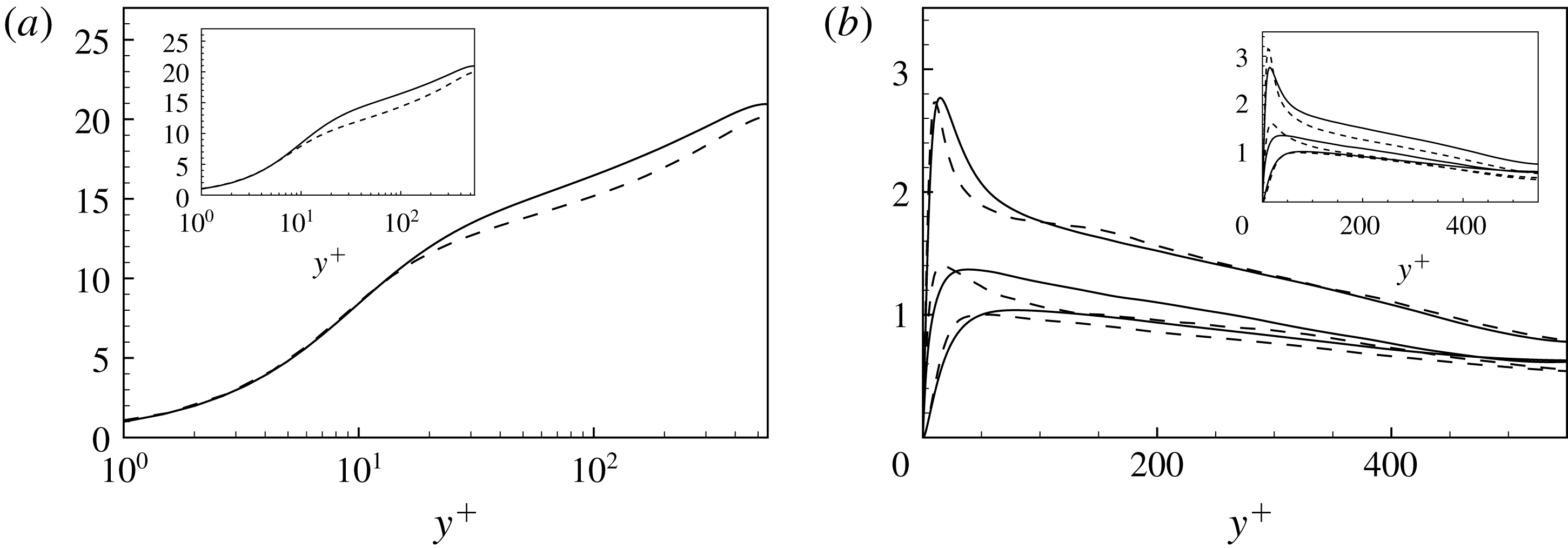
8 Final remarks
Turbulence is widely recognized to be a multilevel and multiscale phenomenon. The nonlinearity of the physical phenomena underlying turbulence gives rise to complex interactions and exchanges of momentum and energy among the different levels and scales composing it. The study of these interactions is then recognized to be fundamental for both theory and modelling. In this context, most of the approaches to turbulence are based on a decomposition of the turbulent field in different contributions. Classical examples of the multilevel and multiscale decomposition of turbulence are the Reynolds and spectral decompositions, respectively. An additional decomposition is based on hierarchies of filter lengths and is given by the large eddy decomposition, thus providing an additional framework for the study of the multiscale feature of turbulence. For a given filter length, turbulence is decomposed in large and small scales, the so-called resolved and subgrid motion. The two ranges of scales interact among themselves and exchange momentum and energy, thus giving rise to a coupling nonlinear term in the equations, the so-called subgrid stress tensor. By varying the filter lengths, the subgrid stresses become generalized central moments of the second order (Germano Reference Germano2012) that can be used to study and model the different parts composing turbulence at different levels. In the present work we address these aspects by proposing a general theoretical framework for a reduced description of the interscale momentum flux and energy exchange given by the subgrid stresses and for their modelling.
The subgrid stresses are classically decomposed into three main contributions representing nonlinear interactions occurring in the large scales, in between large and small scales and finally in the small-scale field,
 $$\begin{eqnarray}\unicode[STIX]{x1D70F}(u_{i},u_{j})=\unicode[STIX]{x1D70F}(\bar{u}_{i},\bar{u}_{j})+[\unicode[STIX]{x1D70F}(\bar{u}_{i},\unicode[STIX]{x1D710}_{j})+\unicode[STIX]{x1D70F}(\unicode[STIX]{x1D710}_{i},\bar{u}_{j})]+\unicode[STIX]{x1D70F}(\unicode[STIX]{x1D710}_{i},\unicode[STIX]{x1D710}_{j}),\end{eqnarray}$$
respectively. Here, we propose an alternative decomposition where two main contributions appear representing interactions of the total velocity field with the large and small scales composing it,
 $$\begin{eqnarray}\unicode[STIX]{x1D70F}(u_{i},u_{j})=[\unicode[STIX]{x1D70F}(\bar{u}_{i},u_{j})+\unicode[STIX]{x1D70F}(u_{i},\bar{u}_{j})]/2+[\unicode[STIX]{x1D70F}(\unicode[STIX]{x1D710}_{i},u_{j})+\unicode[STIX]{x1D70F}(u_{i},\unicode[STIX]{x1D710}_{j})]/2,\end{eqnarray}$$
respectively. Starting from an exact equation connecting the subgrid stresses with the spatial velocity increments between two points (Germano Reference Germano2007),
 $$\begin{eqnarray}\unicode[STIX]{x1D70F}(u_{i},u_{j})=\frac{1}{2}\iint \!G(\boldsymbol{x},\unicode[STIX]{x1D743})G(\boldsymbol{x},\unicode[STIX]{x1D6C8})[u_{i}(\unicode[STIX]{x1D743})-u_{i}(\unicode[STIX]{x1D6C8})][u_{j}(\unicode[STIX]{x1D743})-u_{j}(\unicode[STIX]{x1D6C8})]\,\text{d}\unicode[STIX]{x1D743}\,\text{d}\unicode[STIX]{x1D6C8},\end{eqnarray}$$
we develop a general formalism for the study of the different contributions to the subgrid momentum flux:
 $$\begin{eqnarray}\displaystyle & \displaystyle \unicode[STIX]{x1D70F}(\bar{u}_{i},\bar{u}_{j})=\frac{1}{2}\iint \!G(\boldsymbol{x},\unicode[STIX]{x1D743})G(\boldsymbol{x},\unicode[STIX]{x1D6C8})[\bar{u}_{i}(\unicode[STIX]{x1D743})-\bar{u}_{i}(\unicode[STIX]{x1D6C8})][\bar{u}_{j}(\unicode[STIX]{x1D743})-\bar{u}_{j}(\unicode[STIX]{x1D6C8})]\,\text{d}\unicode[STIX]{x1D743}\,\text{d}\unicode[STIX]{x1D6C8}, & \displaystyle\end{eqnarray}$$
 $$\begin{eqnarray}\displaystyle & \displaystyle \unicode[STIX]{x1D70F}(\bar{u}_{i},\unicode[STIX]{x1D710}_{j})=\frac{1}{2}\iint \!G(\boldsymbol{x},\unicode[STIX]{x1D743})G(\boldsymbol{x},\unicode[STIX]{x1D6C8})[\bar{u}_{i}(\unicode[STIX]{x1D743})-\bar{u}_{i}(\unicode[STIX]{x1D6C8})][\unicode[STIX]{x1D710}_{j}(\unicode[STIX]{x1D743})-\unicode[STIX]{x1D710}_{j}(\unicode[STIX]{x1D6C8})]\,\text{d}\unicode[STIX]{x1D743}\,\text{d}\unicode[STIX]{x1D6C8}, & \displaystyle\end{eqnarray}$$
 $$\begin{eqnarray}\displaystyle & \displaystyle \unicode[STIX]{x1D70F}(\unicode[STIX]{x1D710}_{i},\unicode[STIX]{x1D710}_{j})=\frac{1}{2}\iint \!G(\boldsymbol{x},\unicode[STIX]{x1D743})G(\boldsymbol{x},\unicode[STIX]{x1D6C8})[\unicode[STIX]{x1D710}_{i}(\unicode[STIX]{x1D743})-\unicode[STIX]{x1D710}_{i}(\unicode[STIX]{x1D6C8})][\unicode[STIX]{x1D710}_{j}(\unicode[STIX]{x1D743})-\unicode[STIX]{x1D710}_{j}(\unicode[STIX]{x1D6C8})]\,\text{d}\unicode[STIX]{x1D743}\,\text{d}\unicode[STIX]{x1D6C8}, & \displaystyle\end{eqnarray}$$
 $$\begin{eqnarray}\displaystyle & \displaystyle \unicode[STIX]{x1D70F}(\bar{u}_{i},u_{j})=\frac{1}{2}\iint \!G(\boldsymbol{x},\unicode[STIX]{x1D743})G(\boldsymbol{x},\unicode[STIX]{x1D6C8})[\bar{u}_{i}(\unicode[STIX]{x1D743})-\bar{u}_{i}(\unicode[STIX]{x1D6C8})][u_{j}(\unicode[STIX]{x1D743})-u_{j}(\unicode[STIX]{x1D6C8})]\,\text{d}\unicode[STIX]{x1D743}\,\text{d}\unicode[STIX]{x1D6C8}, & \displaystyle\end{eqnarray}$$
 $$\begin{eqnarray}\displaystyle & \displaystyle \unicode[STIX]{x1D70F}(\unicode[STIX]{x1D710}_{i},u_{j})=\frac{1}{2}\iint \!G(\boldsymbol{x},\unicode[STIX]{x1D743})G(\boldsymbol{x},\unicode[STIX]{x1D6C8})[\unicode[STIX]{x1D710}_{i}(\unicode[STIX]{x1D743})-\unicode[STIX]{x1D710}_{i}(\unicode[STIX]{x1D6C8})][u_{j}(\unicode[STIX]{x1D743})-u_{j}(\unicode[STIX]{x1D6C8})]\,\text{d}\unicode[STIX]{x1D743}\,\text{d}\unicode[STIX]{x1D6C8}. & \displaystyle\end{eqnarray}$$
In the proposed framework, the spatial velocity increment is a central object. By analysing DNS data of a turbulent channel, a rich physics underlying the different contributions to the subgrid stresses is unveiled. We find that the subgrid stresses are dominated by contributions given by the nonlinear phenomena involving the large-scale motion and its interactions with the small-scale field, i.e. the terms
 $$\begin{eqnarray}\unicode[STIX]{x1D70F}(\bar{u}_{i},\bar{u}_{j})\quad [\unicode[STIX]{x1D70F}(\bar{u}_{i},\unicode[STIX]{x1D710}_{j})+\unicode[STIX]{x1D70F}(\unicode[STIX]{x1D710}_{i},\bar{u}_{j})]\quad [\unicode[STIX]{x1D70F}(\bar{u}_{i},u_{j})+\unicode[STIX]{x1D70F}(u_{i},\bar{u}_{j})].\end{eqnarray}$$
Indeed, such terms are those found to contribute mostly to the momentum flux and energy transfer exploited by the subgrid stresses. This is particularly true for not very large filter lengths and away from the wall regions. Interestingly, all the terms contributing to the subgrid stresses show a significant non-Gaussian behaviour in terms of both skewness and kurtosis which is partially reduced by increasing the filter length. By assuming that the filtered velocity increment can be expanded as
 $$\begin{eqnarray}\bar{u}_{i}(\unicode[STIX]{x1D743})-\bar{u}_{i}(\unicode[STIX]{x1D6C8})\approx (\unicode[STIX]{x1D709}_{k}-\unicode[STIX]{x1D702}_{k})\unicode[STIX]{x2202}_{k}\bar{u}_{i},\end{eqnarray}$$
we find that a reduced description for the dominant contributions to the subgrid stresses, terms (8.9), is given by
 $$\begin{eqnarray}\displaystyle & \displaystyle \unicode[STIX]{x1D70F}(\bar{u}_{i},\bar{u}_{j})\approx -\unicode[STIX]{x1D708}_{kj}^{(g)}\unicode[STIX]{x2202}_{k}\bar{u}_{i}-\unicode[STIX]{x1D708}_{ki}^{(g)}\unicode[STIX]{x2202}_{k}\bar{u}_{j}, & \displaystyle\end{eqnarray}$$
 $$\begin{eqnarray}\displaystyle & \displaystyle [\unicode[STIX]{x1D70F}(\bar{u}_{i},\unicode[STIX]{x1D710}_{j})+\unicode[STIX]{x1D70F}(\unicode[STIX]{x1D710}_{i},\bar{u}_{j})]/2\approx -\unicode[STIX]{x1D708}_{kj}^{(cross)}\unicode[STIX]{x2202}_{k}\bar{u}_{i}-\unicode[STIX]{x1D708}_{ki}^{(cross)}\unicode[STIX]{x2202}_{k}\bar{u}_{j}, & \displaystyle\end{eqnarray}$$
 $$\begin{eqnarray}\displaystyle & \displaystyle [\unicode[STIX]{x1D70F}(\bar{u}_{i},u_{j})+\unicode[STIX]{x1D70F}(u_{i},\bar{u}_{j})]/2\approx -\unicode[STIX]{x1D708}_{kj}\unicode[STIX]{x2202}_{k}\bar{u}_{i}-\unicode[STIX]{x1D708}_{ki}\unicode[STIX]{x2202}_{k}\bar{u}_{j}, & \displaystyle\end{eqnarray}$$
where the associated turbulent viscosities are tensors given by
 $$\begin{eqnarray}\displaystyle & \displaystyle \unicode[STIX]{x1D708}_{ki}^{(g)}=-\frac{1}{4}\unicode[STIX]{x2202}_{h}\bar{u}_{i}\iint \!G(\boldsymbol{x},\unicode[STIX]{x1D743})G(\boldsymbol{x},\unicode[STIX]{x1D6C8})(\unicode[STIX]{x1D709}_{k}-\unicode[STIX]{x1D702}_{k})(\unicode[STIX]{x1D709}_{h}-\unicode[STIX]{x1D702}_{h})\,\text{d}\unicode[STIX]{x1D743}\,\text{d}\unicode[STIX]{x1D6C8}, & \displaystyle\end{eqnarray}$$
 $$\begin{eqnarray}\displaystyle & \displaystyle \unicode[STIX]{x1D708}_{ki}^{(cross)}=-\frac{1}{4}\iint \!G(\boldsymbol{x},\unicode[STIX]{x1D743})G(\boldsymbol{x},\unicode[STIX]{x1D6C8})[\unicode[STIX]{x1D709}_{k}-\unicode[STIX]{x1D702}_{k}][\unicode[STIX]{x1D710}_{i}(\unicode[STIX]{x1D743})-\unicode[STIX]{x1D710}_{i}(\unicode[STIX]{x1D6C8})]\,\text{d}\unicode[STIX]{x1D743}\,\text{d}\unicode[STIX]{x1D6C8}, & \displaystyle\end{eqnarray}$$
 $$\begin{eqnarray}\displaystyle & \displaystyle \unicode[STIX]{x1D708}_{ki}=-\frac{1}{4}\iint \!G(\boldsymbol{x},\unicode[STIX]{x1D743})G(\boldsymbol{x},\unicode[STIX]{x1D6C8})[\unicode[STIX]{x1D709}_{k}-\unicode[STIX]{x1D702}_{k}][u_{i}(\unicode[STIX]{x1D743})-u_{i}(\unicode[STIX]{x1D6C8})]\,\text{d}\unicode[STIX]{x1D743}\,\text{d}\unicode[STIX]{x1D6C8}. & \displaystyle\end{eqnarray}$$
These three viscosities are strictly related each other by
 $$\begin{eqnarray}\unicode[STIX]{x1D708}_{ki}=\unicode[STIX]{x1D708}_{ki}^{(g)}+\unicode[STIX]{x1D708}_{ki}^{(cross)},\end{eqnarray}$$
thus highlighting that the most significant term of the new decomposition,
 $[\unicode[STIX]{x1D70F}(\bar{u}_{i},u_{j})+\unicode[STIX]{x1D70F}(u_{i},\bar{u}_{j})]/2$
, together with its reduced description given by the turbulent viscosity tensor,
 $\unicode[STIX]{x1D708}_{ki}$
, takes into account the two most significant terms of the old decomposition. The above equations also highlight that every decomposition of the subgrid stresses involving interactions between large and small scales is naturally approximated by a turbulent viscosity tensor formalism based on the velocity increments which is then recognized to be a peculiar property of small-scale stresses in turbulence. Accordingly, we use DNS data of a turbulent channel flow to analyse the complex physics unveiled by the tensorial viscosity approach. The observed behaviour of the different components of the subgrid viscosity tensor, in terms of intensity, distribution, skewness and kurtosis, highlights complex anisotropic and inhomogeneous features that are actually missed in more classical scalar turbulent viscosity approaches based on the Kolmogorov hypothesis of isotropy of the small scales of turbulence. Hence, the introduced turbulent viscosity formalism appears as a valid alternative candidate for the development of theories on the interscale momentum and energy transfer in turbulence.
To further support the potentiality of the developed theoretical framework, we also show how the turbulent viscosity tensor formalism based on the velocity increments can be used to derive alternative turbulence closures in a context of LES. The procedure leads to an anisotropic turbulent viscosity model that reads
 $$\begin{eqnarray}\unicode[STIX]{x1D70F}(u_{i},u_{j})=-\unicode[STIX]{x1D708}_{kj}\unicode[STIX]{x2202}_{k}\bar{u}_{i}-\unicode[STIX]{x1D708}_{ki}\unicode[STIX]{x2202}_{k}\bar{u}_{j},\end{eqnarray}$$
with
 $$\begin{eqnarray}\unicode[STIX]{x1D708}_{ki}=\frac{1}{2\unicode[STIX]{x1D6FA}}{\mathcal{I}}_{kh}^{\prime }\unicode[STIX]{x2202}_{h}\bar{u}_{i},\end{eqnarray}$$
at the first-order approximation, and
 $$\begin{eqnarray}\unicode[STIX]{x1D708}_{ki}=\frac{1}{2\unicode[STIX]{x1D6FA}}{\mathcal{I}}_{kh}^{\prime }\unicode[STIX]{x2202}_{h}\bar{u}_{i}(\boldsymbol{x})-\frac{1}{4\unicode[STIX]{x1D6FA}}{\mathcal{M}}_{khl}\unicode[STIX]{x2202}_{hl}\bar{u}_{i}(\boldsymbol{x}),\end{eqnarray}$$
at the second order. The models are based on the filtered velocity derivatives and on the second- and third-order inertial properties of the grid elements. The basic idea is that the structure of the computational element can be used to model the unknown distribution of the subgrid velocity field within it. Indeed, not only the size but also the anisotropic feature of the unresolved motion significantly depends on the geometrical properties of the computational volume. This is simply due to the fact that the integration volume together with the filter kernel in the case of explicit filters is responsible for the definition of the subgrid field itself by splitting the velocity field into large and small scales. Hence, the prediction of the subgrid velocity distribution within the computational volume given by the filtered velocity derivatives,
 $\unicode[STIX]{x2202}_{h}\bar{u}_{i}$
and
 $\unicode[STIX]{x2202}_{hl}\bar{u}_{i}$
, can be improved by using the known geometrical properties of the computational volume. These aspects are particularly relevant when the geometrical features of the computational mesh conform with the peculiar features of the problem, i.e. when the inhomogeneous distribution of resolution is able to take into account flow regions characterized by relatively small scales (e.g. near-wall turbulence) and when the anisotropy of the computational elements is able to conform with the anisotropies of the flow (e.g. such as the anisotropy induced by the presence of a predominant flow direction imposed by the geometry of the problem). This kind of information is carried by the computational grid and can be grasped by the proposed modelling approach.
An interesting result of the model formulation is that it allows one to model the normal subgrid stresses and, hence, to give a measure of the subgrid kinetic energy. An additional outcome of the proposed model is given by the fact that it provides a rigorous definition of characteristic lengths for the subgrid stresses,
 $$\begin{eqnarray}(\unicode[STIX]{x1D6E5}_{ij})^{2}=\frac{1}{\unicode[STIX]{x1D6FA}}\int _{\unicode[STIX]{x1D6FA}}\!(\unicode[STIX]{x1D709}_{h}-x_{h})(\unicode[STIX]{x1D709}_{k}-x_{k})\,\text{d}\unicode[STIX]{x1D743},\end{eqnarray}$$
which can be computed in every type of computational elements, thus overcoming the rather elusive definition of filter length commonly employed in more classical subgrid models. By means of a contraction of the tensorial formulation, it is finally pointed out that the above definition can be used also to compute a scalar subgrid scale to be used in isotropic subgrid-scale models when applied to complex unstructured computational grids.
In barycentric structured Cartesian grids, the present approximation of the subgrid viscosity reduces to the viscosity of the gradient model. This modelling approach is widely recognized to have a good correlation with the actual subgrid stresses but also to suffer from numerical stability issues. To solve this problem, several approaches have been introduced in the literature and found to properly work. Here, in order to emphasize the anisotropic character of the proposed closures, we developed an alternative modulation technique based on a tensorial dynamic procedure for the evolution of the model constants. The generality of the procedure is such that it can be employed also in other types of models. Preliminary analysis in a turbulent channel shows promising results, thus forming the basis for future assessments of the model performances in more complex flow where non-Cartesian grids are demanded and the present closures differ from the gradient model approximation.
Appendix A. On the subgrid flux associated with the scalar
 $\unicode[STIX]{x1D703}$

Let us consider the subgrid flux associated with the scalar field
 $\unicode[STIX]{x1D703}$
,
 $$\begin{eqnarray}\unicode[STIX]{x1D70F}(\unicode[STIX]{x1D703},u_{j})=\overline{\unicode[STIX]{x1D703}u_{j}}-\bar{\unicode[STIX]{x1D703}}\bar{u}_{j},\end{eqnarray}$$
where the overbar stands for a generic filter operator that can be represented as
 $$\begin{eqnarray}\bar{\unicode[STIX]{x1D703}}=\int G(\boldsymbol{x},\unicode[STIX]{x1D743})\unicode[STIX]{x1D703}(\unicode[STIX]{x1D743})\,\text{d}\unicode[STIX]{x1D743}\end{eqnarray}$$
with
 $$\begin{eqnarray}\int G(\boldsymbol{x},\unicode[STIX]{x1D743})\,\text{d}\unicode[STIX]{x1D743}=1\;.\end{eqnarray}$$
Let us now express both the scalar and velocity fields as the sum of two terms
 $$\begin{eqnarray}\unicode[STIX]{x1D703}=\bar{\unicode[STIX]{x1D703}}+\unicode[STIX]{x1D717}\quad u_{j}=\bar{u}_{j}+\unicode[STIX]{x1D710}_{j},\end{eqnarray}$$
where
 $\unicode[STIX]{x1D717}$
and
 $\unicode[STIX]{x1D710}$
are the fluctuations associated with the averaging operator
 $G$
. If we apply the Galilean invariant decomposition of the subgrid flux (Germano Reference Germano1986), we can write
 $$\begin{eqnarray}\unicode[STIX]{x1D70F}(\unicode[STIX]{x1D703},u_{j})=\unicode[STIX]{x1D70F}(\bar{\unicode[STIX]{x1D703}},u_{j})+\unicode[STIX]{x1D70F}(\unicode[STIX]{x1D717},u_{j}),\end{eqnarray}$$
where
 $$\begin{eqnarray}\left.\begin{array}{@{}c@{}}\unicode[STIX]{x1D70F}(\bar{\unicode[STIX]{x1D703}},u_{j})=\overline{\bar{\unicode[STIX]{x1D703}}u_{j}}-\bar{\bar{\unicode[STIX]{x1D703}}}\bar{u}_{j}\\ \unicode[STIX]{x1D70F}(\unicode[STIX]{x1D717},u_{j})=\overline{\unicode[STIX]{x1D717}u_{j}}-\bar{\unicode[STIX]{x1D717}}\bar{u}_{j}\end{array}\right\}\end{eqnarray}$$
and we remark that this decomposition is Galilean invariant, due to the fact that it is composed of Galilean invariant terms. A further decomposition of the subgrid flux leads to
 $$\begin{eqnarray}\unicode[STIX]{x1D70F}(\unicode[STIX]{x1D703},u_{j})=\unicode[STIX]{x1D70F}(\bar{\unicode[STIX]{x1D703}},\bar{u}_{j})+\unicode[STIX]{x1D70F}(\bar{\unicode[STIX]{x1D703}},\unicode[STIX]{x1D710})+\unicode[STIX]{x1D70F}(\unicode[STIX]{x1D717},\bar{u}_{j})+\unicode[STIX]{x1D70F}(\unicode[STIX]{x1D717},\unicode[STIX]{x1D710}_{j}).\end{eqnarray}$$
We remark that the total subgrid flux and its decompositions are equivalently given by a double convolution integral of the scalar and velocity increments between two points (Germano Reference Germano2007). For the first term on the right-hand side of (A 5) and (A 7), this relation reads
 $$\begin{eqnarray}\displaystyle & \displaystyle \unicode[STIX]{x1D70F}(\bar{\unicode[STIX]{x1D703}},u_{j})=\frac{1}{2}\iint \!G(\boldsymbol{x},\unicode[STIX]{x1D743})G(\boldsymbol{x},\unicode[STIX]{x1D6C8})[\bar{\unicode[STIX]{x1D703}}(\unicode[STIX]{x1D743})-\bar{\unicode[STIX]{x1D703}}(\unicode[STIX]{x1D6C8})][u_{j}(\unicode[STIX]{x1D743})-u_{j}(\unicode[STIX]{x1D6C8})]\,\text{d}\unicode[STIX]{x1D743}\,\text{d}\unicode[STIX]{x1D6C8}, & \displaystyle\end{eqnarray}$$
 $$\begin{eqnarray}\displaystyle & \displaystyle \unicode[STIX]{x1D70F}(\bar{\unicode[STIX]{x1D703}},\bar{u}_{j})=\frac{1}{2}\iint \!G(\boldsymbol{x},\unicode[STIX]{x1D743})G(\boldsymbol{x},\unicode[STIX]{x1D6C8})[\bar{\unicode[STIX]{x1D703}}(\unicode[STIX]{x1D743})-\bar{\unicode[STIX]{x1D703}}(\unicode[STIX]{x1D6C8})][\bar{u}_{j}(\unicode[STIX]{x1D743})-\bar{u}_{j}(\unicode[STIX]{x1D6C8})]\,\text{d}\unicode[STIX]{x1D743}\,\text{d}\unicode[STIX]{x1D6C8}, & \displaystyle\end{eqnarray}$$
which clearly evidence the Galilean invariance of the different terms. The two decompositions given by (A 5) and (A 7) suggest two possible approximations of the total subgrid flux:
 $$\begin{eqnarray}\displaystyle & \displaystyle \unicode[STIX]{x1D70F}(\unicode[STIX]{x1D703},u_{j})\approx \unicode[STIX]{x1D70F}(\bar{\unicode[STIX]{x1D703}},u_{j}), & \displaystyle\end{eqnarray}$$
 $$\begin{eqnarray}\displaystyle & \displaystyle \unicode[STIX]{x1D70F}(\unicode[STIX]{x1D703},u_{j})\approx \unicode[STIX]{x1D70F}(\bar{\unicode[STIX]{x1D703}},\bar{u}_{j}), & \displaystyle\end{eqnarray}$$
respectively. We remark that the approximation of the subgrid flux decomposition (A 11) directly recovers the approach given by the scale similarity models, i.e.
 $$\begin{eqnarray}\unicode[STIX]{x1D70F}(\unicode[STIX]{x1D703},u_{j})\approx \unicode[STIX]{x1D70F}(\bar{\unicode[STIX]{x1D703}},\bar{u}_{j})=\overline{\bar{\unicode[STIX]{x1D703}}\bar{u}_{j}}-\bar{\bar{\unicode[STIX]{x1D703}}},\bar{\bar{u}}_{j}.\end{eqnarray}$$
If we now further assume that the LES averaged values
 $\bar{\unicode[STIX]{x1D703}}$
and
 $\bar{u}_{j}$
are sufficiently smooth at the LES scale, we can consider the following expansion:
 $$\begin{eqnarray}\displaystyle & \displaystyle \bar{\unicode[STIX]{x1D703}}(\unicode[STIX]{x1D743})-\bar{\unicode[STIX]{x1D703}}(\unicode[STIX]{x1D6C8})\approx (\unicode[STIX]{x1D709}_{k}-\unicode[STIX]{x1D702}_{k})\unicode[STIX]{x2202}_{k}\bar{\unicode[STIX]{x1D703}}, & \displaystyle\end{eqnarray}$$
 $$\begin{eqnarray}\displaystyle & \displaystyle \bar{u}_{j}(\unicode[STIX]{x1D743})-\bar{u}_{j}(\unicode[STIX]{x1D6C8})\approx (\unicode[STIX]{x1D709}_{k}-\unicode[STIX]{x1D702}_{k})\unicode[STIX]{x2202}_{k}\bar{u}_{j} & \displaystyle\end{eqnarray}$$
to show that approximation (A 11) reduces also the generalized form of gradient model for the subgrid flux:
 $$\begin{eqnarray}\unicode[STIX]{x1D70F}(\unicode[STIX]{x1D703},u_{j})\approx \unicode[STIX]{x1D70F}(\bar{\unicode[STIX]{x1D703}},\bar{u}_{j})\approx -\unicode[STIX]{x1D708}_{kj}^{(g)}\unicode[STIX]{x2202}_{k}\bar{\unicode[STIX]{x1D703}},\end{eqnarray}$$
where the associated subgrid viscosity is a tensor given by
 $$\begin{eqnarray}\unicode[STIX]{x1D708}_{kj}^{(g)}=-\unicode[STIX]{x1D70F}(x_{k},x_{h})\unicode[STIX]{x2202}_{h}\bar{u}_{j}\end{eqnarray}$$
and
 $$\begin{eqnarray}\unicode[STIX]{x1D70F}(x_{k},x_{h})=\frac{1}{2}\iint \!G(\boldsymbol{x},\unicode[STIX]{x1D743})G(\boldsymbol{x},\unicode[STIX]{x1D6C8})(\unicode[STIX]{x1D709}_{k}-\unicode[STIX]{x1D702}_{k})(\unicode[STIX]{x1D709}_{h}-\unicode[STIX]{x1D702}_{h})\,\text{d}\unicode[STIX]{x1D743}\,\text{d}\unicode[STIX]{x1D6C8}.\end{eqnarray}$$
When considering a Cartesian control volume and a top-hat filter, we have
 $$\begin{eqnarray}\unicode[STIX]{x1D70F}(x_{k},x_{h})={\textstyle \frac{1}{12}}\unicode[STIX]{x1D6E5}_{h}^{2}\unicode[STIX]{x1D6FF}_{kh},\end{eqnarray}$$
and the generalized gradient model approximation for the subgrid flux (A 15) recovers the classical gradient model:
 $$\begin{eqnarray}\unicode[STIX]{x1D70F}(\unicode[STIX]{x1D703},u_{j})\approx \unicode[STIX]{x1D70F}(\bar{\unicode[STIX]{x1D703}},\bar{u}_{j})\approx \left({\textstyle \frac{1}{12}}\unicode[STIX]{x1D6E5}_{k}^{2}\unicode[STIX]{x2202}_{k}\bar{u}_{j}\right)\unicode[STIX]{x2202}_{k}\bar{\unicode[STIX]{x1D703}}.\end{eqnarray}$$
Alternatively, by applying expansion (A 13) to the approximation given by the first decomposition of the subgrid flux (A 10) we have
 $$\begin{eqnarray}\unicode[STIX]{x1D70F}(\unicode[STIX]{x1D703},u_{j})\approx \unicode[STIX]{x1D70F}(\bar{\unicode[STIX]{x1D703}},u_{j})\approx -\unicode[STIX]{x1D708}_{kj}\unicode[STIX]{x2202}_{k}\bar{\unicode[STIX]{x1D703}},\end{eqnarray}$$
where the associated subgrid viscosity is again a tensor given by
 $$\begin{eqnarray}\unicode[STIX]{x1D708}_{kj}=-\unicode[STIX]{x1D70F}(x_{k},u_{j})\end{eqnarray}$$
and
 $$\begin{eqnarray}\unicode[STIX]{x1D70F}(x_{k},u_{j})=\frac{1}{2}\iint \!G(\boldsymbol{x},\unicode[STIX]{x1D743})G(\boldsymbol{x},\unicode[STIX]{x1D6C8})(\unicode[STIX]{x1D709}_{k}-\unicode[STIX]{x1D702}_{k})[u_{j}(\unicode[STIX]{x1D743})-u_{j}(\unicode[STIX]{x1D6C8})]\,\text{d}\unicode[STIX]{x1D743}\,\text{d}\unicode[STIX]{x1D6C8}.\end{eqnarray}$$
Equation (A 22) further supports the idea that a subgrid viscosity tensor based on velocity increments is a natural approximation of multiscale phenomena of momentum and scalar flux originating from interactions between scales of different sizes. By following the reasoning reported in § 6, the reduced description given by the subgrid viscosity tensor (A 22) can also be used to derive turbulence closures as
 $$\begin{eqnarray}\displaystyle & \displaystyle \unicode[STIX]{x1D708}_{kj}=\frac{1}{\unicode[STIX]{x1D6FA}}{\mathcal{I}}_{kh}^{\prime }\unicode[STIX]{x2202}_{h}\bar{u}_{j}, & \displaystyle\end{eqnarray}$$
 $$\begin{eqnarray}\displaystyle & \displaystyle \unicode[STIX]{x1D708}_{kj}=\frac{1}{\unicode[STIX]{x1D6FA}}{\mathcal{I}}_{kh}^{\prime }\unicode[STIX]{x2202}_{h}\bar{u}_{j}-\frac{1}{2\unicode[STIX]{x1D6FA}}{\mathcal{M}}_{khl}\unicode[STIX]{x2202}_{hl}\bar{u}_{j} & \displaystyle\end{eqnarray}$$
for the first- and second-order approximations, respectively. In closing this appendix, let us point out that the subgrid viscosity approximations given by the present and gradient modelling approach, equations (A 23), (A 24) and (A 16), respectively, only depend on the velocity field
 $u_{j}$
and on the LES filtering operator
 $G$
and they have no relations to the scalar field
 $\unicode[STIX]{x1D703}$
. As such they are peculiar to the given turbulent velocity field. Accordingly with the main outcomes of the work, the proposed models can be understood as a refinement of the classical gradient approach to the modelling of the subgrid flux in complex flows where unstructured irregular computational grids are commonly used.