3.1 Evolution of the bed surface

The bed surface, namely the (fictitious) solid–fluid interface, can be defined on the basis of the sediment volume concentration, hereafter referred to as the particle volume fraction and denoted by $\unicode[STIX]{x1D719}_{s}$ , which is zero far away from the bottom and abruptly increases at the bed. Hence, the bed surface is identified by points where $\unicode[STIX]{x1D719}_{s}$ reaches a threshold value. Similarly, in laboratory experiments, the bed–flow interface is often detected by means of an image analysis procedure, thresholding the side view frames of the bed (e.g. Aussillous et al. Reference Aussillous, Chauchat, Pailha, Médale and Guazzelli2013). In fact, the greyscale image contrast is highly correlated with $\unicode[STIX]{x1D719}_{s}$ . This approach was successfully reproduced numerically by Kidanemariam & Uhlmann (Reference Kidanemariam and Uhlmann2014a ) who considered the threshold value $\unicode[STIX]{x1D719}_{s}=0.1$ . Kidanemariam & Uhlmann (Reference Kidanemariam and Uhlmann2014a ) defined a sample volume of size $\unicode[STIX]{x0394}x_{1}^{\ast }\times \unicode[STIX]{x0394}x_{2}^{\ast }\times L_{x_{3}}^{\ast }$ over which the particle volume fraction was evaluated. Therefore, the dependency of $\unicode[STIX]{x1D719}_{s}$ on $x_{3}^{\ast }$ was neglected and the bed profile, $\unicode[STIX]{x1D702}_{\unicode[STIX]{x1D719}}^{\ast }(x_{1}^{\ast },t^{\ast })$ , was obtained.

Another approach is also presently considered which was first adopted by Mazzuoli et al. (Reference Mazzuoli, Blondeaux, Simeonov and Calantoni2017) to detect the bed/flow interface. Since spheres are presently not set into suspension, they remain in enduring contact throughout their motion and the bed surface can be thus unambiguously identified by the centres of the spheres on top of others, which are hereafter referred to as top-layer particles (cf. dark grey spheres in figure 1). The $i$ th sphere ( $i=1,\ldots ,N_{s}$ ) belongs to the top layer if no other sphere centres above the $i$ th one lie inside the solid angle of magnitude  $\unicode[STIX]{x1D6FA}=(2-\sqrt{3})\unicode[STIX]{x03C0}$  sr (where sr denotes steradian) with respect to the bottom normal. Then, if this condition is fulfilled, the Boolean function ${\mathcal{E}}_{i}$ associated with the $i$ th particle is equal to 1, otherwise it is equal to 0. Therefore, the bed surface is defined as the function interpolating the centres of the spheres characterised by ${\mathcal{E}}=1$ , and is denoted by $\unicode[STIX]{x1D702}^{\ast }(x_{1}^{\ast },x_{3}^{\ast },t^{\ast })$ . Such a definition circumvents the matter of defining a threshold and allows us also to study three-dimensional patterns. The patterns observed for the present values of the parameters do not show an appreciable dependency on the spanwise coordinate. Additionally, the bed profile $\unicode[STIX]{x1D702}_{{\mathcal{E}}}^{\ast }$ , defined as equal to $\langle \unicode[STIX]{x1D702}^{\ast }\rangle _{x_{3}}$ , is found practically to collapse on $\unicode[STIX]{x1D702}_{\unicode[STIX]{x1D719}}^{\ast }$ once it is shifted vertically upward by a constant value ${\sim}0.8d^{\ast }$ (cf. figure 3). Since the position of the bed profile is analogously detected by the two procedures, henceforth the profile $\unicode[STIX]{x1D702}_{\unicode[STIX]{x1D719}}^{\ast }$ is considered.

Figure 3.

Comparison between the bed profiles $\unicode[STIX]{x1D702}_{{\mathcal{E}}}$ (red line) and $\unicode[STIX]{x1D702}_{\unicode[STIX]{x1D719}}$ (black line) at an instant of run 1 when rolling-grain ripples are present.

In the simulations, the average bed elevation $\langle \unicode[STIX]{x1D702}_{\unicode[STIX]{x1D719}}\rangle _{x_{1}}$ initially decreases as an effect of the settlement and compaction of the granular bed (not shown here). Then, after a few oscillation periods $\langle \unicode[STIX]{x1D702}_{\unicode[STIX]{x1D719}}\rangle _{x_{1}}$  asymptotically reaches a constant value approximately equal to $13.83d^{\ast }$ and $12.12d^{\ast }$ for runs 1 and 2, respectively, superimposed only by small fluctuations of order $O(10^{-2})d^{\ast }$ , which are related to the different phases of the wave cycle. Correspondingly, the solid volume fraction, $\unicode[STIX]{x1D719}_{s}$ , in the region between the bottom and the surface layers of particles does not show significant temporal fluctuations and attains an average value of 0.49 for both runs. Instead, figure 4 shows the space–time development of the fluctuations of the bed profile about the average bed elevation, i.e. $\unicode[STIX]{x1D702}_{\unicode[STIX]{x1D719}}=\unicode[STIX]{x1D702}_{\unicode[STIX]{x1D719}}-\langle \unicode[STIX]{x1D702}_{\unicode[STIX]{x1D719}}\rangle _{x_{1}}$ , for runs 1 and 2. While bedforms emerge in the second half of run 1, in run 2 the presence of persistent patterns is difficult to detect by visual inspection of figure 4(b). The root mean square (r.m.s.) of $\unicode[STIX]{x1D702}_{\unicode[STIX]{x1D719}}^{\prime }$ , $\unicode[STIX]{x1D702}_{rms}$ , increases with time in both runs (cf. figure 5), whilst the amplitude of the fluctuations attained at the end of run 2 barely reaches $0.1d^{\ast }$ (three times smaller than that of run 1). In run 1, the linear regression of $\ln \unicode[STIX]{x1D702}_{rms}$ (red solid line in figure 5 a) shows that $\unicode[STIX]{x1D702}_{rms}$ grows exponentially. Moreover, the regression of relative maxima and minima of $\unicode[STIX]{x1D702}_{rms}$ computed for each half-period (indicated with dashed lines in figure 5 a) preserves the exponent of the mean trend. Thus, the amplification of half-period fluctuations of the bed surface, normalised by the particle diameter, can be approximated by the expression:

(3.1) $$\begin{eqnarray}{\mathcal{A}}_{\unicode[STIX]{x1D702}}=(a_{max}-a_{min})\text{e}^{b\,t},\end{eqnarray}$$

where $b=1.46\times 10^{-2}$ and the factors $a_{max}=4.98\times 10^{-2}$ and $a_{min}=3.38\times 10^{-2}$ refer to the average upper and lower bounds of $\unicode[STIX]{x1D702}_{rms}$ . In other words, the rate of coarsening of the ripples is directly proportional to the amplitude of the ripples. On the other hand, in run 2, the time development of $\unicode[STIX]{x1D702}_{rms}$ is not monotonic and the mean growth is slower than that observed for simulation 1 (cf. figure 5 b). It is likely that, after a much larger number of oscillation periods, the formation of ripples could be observed more clearly also in case 2, but this would require formidable computational and wall-clock times which are at the moment out of reach.

Figure 4.

Spatio-temporal development of the fluctuations of the bed profile about the average bed elevation, $\unicode[STIX]{x1D702}_{\unicode[STIX]{x1D719}}^{\prime \ast }/d^{\ast }$ , for run 1 (a) and run 2 (b).

Figure 5.

The diagrams in (a) and (b) show the root mean square of the spatial fluctuations of the bed profile plotted versus time for simulations 1 and 2, respectively. The thick solid (red) lines are the regression curves $a\exp (b\,t)$ , where $a=0.040$ , $b=1.46\times 10^{-2}$ for run 1 and $a=0.046$ , $b=4.45\times 10^{-3}$ for run 2. Dashed (red) lines in (a) are obtained for $a=a_{min}=0.034$ and $a=a_{max}=0.050$ . The inset in (a) highlights the exponential trend of $\unicode[STIX]{x1D702}_{rms}$ using semi-logarithmic axis scale.

Figure 6.

(a,b) Absolute values of four Fourier modes of the bed profile plotted versus time for simulations 1 and 2, respectively. Red, blue, black and magenta lines correspond to the second, third, fourth and fifth modes of the bed profile, respectively.

Figure 7.

Dominant wavelength of the bed profile computed as a function of time for runs 1 (a) and 2 (b).

To detect the wavelength of ripples as a function of time, the bed profile is expanded in Fourier series and the absolute value and the growth rate of each term of the series are investigated. It is evident that the wavenumbers $k^{\ast }\unicode[STIX]{x1D6FF}^{\ast }=0.47$ and $k^{\ast }\unicode[STIX]{x1D6FF}^{\ast }=0.25$ dominate the spectra of $\unicode[STIX]{x1D702}_{\unicode[STIX]{x1D719}}^{\prime }$ at the end of runs 1 and $2$ , respectively (cf. figure 6). However, since modes are still evolving at the end of each run, an equilibrium condition is not reached and the simulation time is not sufficient to describe the complete evolution of individual modes. Alternatively, the dominant wavelength can be defined as two times the space lag, $\unicode[STIX]{x1D706}_{\unicode[STIX]{x1D702}}^{\ast }$ , at which the absolute value of the two-point correlation function of $\unicode[STIX]{x1D702}_{\unicode[STIX]{x1D719}}^{\prime \ast }$ attains the first maximum value (Kidanemariam & Uhlmann Reference Kidanemariam and Uhlmann2017). The result of this procedure is shown in figure 7. As predicted by the Fourier analysis, the dominant wavelength for the second half of simulation 1 corresponds to the wavenumber $k^{\ast }\unicode[STIX]{x1D6FF}^{\ast }=0.47$ ( $\unicode[STIX]{x1D706}_{\unicode[STIX]{x1D702}}^{\ast }=13\unicode[STIX]{x1D6FF}^{\ast }$ ) while for the last ${\sim}6$ oscillation periods of simulation 2 patterns are characterised by the wavenumber $k^{\ast }\unicode[STIX]{x1D6FF}^{\ast }=0.25$ ( $\unicode[STIX]{x1D706}_{\unicode[STIX]{x1D702}}^{\ast }=25\unicode[STIX]{x1D6FF}^{\ast }$ ). The values of $\unicode[STIX]{x1D706}_{\unicode[STIX]{x1D702}}^{\ast }$ can be compared with the results of the experiments carried out by Blondeaux et al. (Reference Blondeaux, Sleath and Vittori1988) for similar values of the parameters and with those obtained by linear stability analysis by Blondeaux (Reference Blondeaux1990). It is found that the values of $\unicode[STIX]{x1D706}_{\unicode[STIX]{x1D702}}^{\ast }$ in the current simulations are comparable to the wavelengths of the first emerging ripples observed in the laboratory. At this stage it is worthwhile to remark on the importance of this result, since a natural very complex phenomenon has been reproduced by a very simplified, although numerically challenging, system, which indicates that the basic process leading to the formation of ripples is somewhat robust. In particular, for the experiment reproduced by run 1, Blondeaux (Reference Blondeaux1990) observed $\unicode[STIX]{x1D706}_{\unicode[STIX]{x1D702}}^{\ast }=25\unicode[STIX]{x1D6FF}^{\ast }$ ( $96d^{\ast }$ ) while for the case simulated by run 2 the value of $\unicode[STIX]{x1D706}_{\unicode[STIX]{x1D702}}^{\ast }$ was approximately equal to $26\unicode[STIX]{x1D6FF}^{\ast }$ ( $108d^{\ast }$ ). Similar results are predicted by means of linear stability analysis following the approach of Blondeaux (Reference Blondeaux1990) ( $\unicode[STIX]{x1D706}_{\unicode[STIX]{x1D702}}^{\ast }=23\unicode[STIX]{x1D6FF}^{\ast }$ for run 1 and $\unicode[STIX]{x1D706}_{\unicode[STIX]{x1D702}}^{\ast }=22\unicode[STIX]{x1D6FF}^{\ast }$ for run 2). Rousseaux et al. (Reference Rousseaux, Stegner and Wesfreid2004a ) carried out experiments also exploring the region of the parameter space where runs 1 and 2 lie and observed the first measured wavelengths $\unicode[STIX]{x1D706}_{\unicode[STIX]{x1D702}}^{\ast }\sim 20\unicode[STIX]{x1D6FF}^{\ast }$ and $\unicode[STIX]{x1D706}_{\unicode[STIX]{x1D702}}^{\ast }\sim 25\unicode[STIX]{x1D6FF}^{\ast }$ , respectively. Therefore, the wavelength of ripples simulated in run 1 is smaller than the wavelength observed experimentally. Such a discrepancy can be due to several reasons mostly associated with the modelling of particle–particle interactions. The significance of the role of sediment friction in the formation of patterns was emphasised by Moon, Swift & Swinney (Reference Moon, Swift and Swinney2004). Indeed, sand grains can have irregular shapes and, consequently, more than one point of contact during a binary collision, which allow them to transfer linear and angular momentum more efficiently than spheres. Moreover, the sensitivity of sediment dynamics to the contact is enhanced if particles roll over each other (enduring contact) rather than colliding. The particles of run 1 behave like finer sand grains, since, based on the experimental results of Rousseaux et al. (Reference Rousseaux, Stegner and Wesfreid2004a ), the first measured wavelength tends to increase monotonically with increasing size of the sediments and because spherical particles are statistically set into motion more easily and undergo larger excursions than sand grains of irregular shape. On the other hand, figure 6(a) shows that the modes associated with the wavenumbers $k^{\ast }\unicode[STIX]{x1D6FF}^{\ast }=0.35$ and $k^{\ast }\unicode[STIX]{x1D6FF}^{\ast }=0.24$ grow at approximately the same rate as the dominant mode in the last periods of run 1 and it is possible that the four ripples of figure 2 might merge after a certain time.

Figure 8.

Bed profile, $\unicode[STIX]{x1D702}_{\unicode[STIX]{x1D719}}$ , (a) and bed slope (b) at different phases of a wave cycle when rolling-grain ripples are formed. Black lines refer to instants $t=136.7$ (solid, thick), $t=137.4$ (dashed, thin), $t=138.2$ (solid, thin) and $t=139.0$ (dashed, thick) while the mean flow is directed from right to left. Red lines refer to instants $t=139.8$ (solid, thick), $t=140.6$ (dashed, thin), $t=141.4$ (solid, thin), $t=142.2$ (dashed, thick) during which the mean flow is directed from left to right.

Figure 9.

Spectra of the bed profile computed at the phases indicated in figure 8 for run 1. The solid (blue) line indicates the spectrum of the simplified configuration sketched in the small inset of the figure with periodic (blue) straight lines.

Even though the ripples of run 1 do not really drift in the streamwise direction, their crests migrate to and fro by several sphere diameters. Therefore, as shown in figure 8, ripple shape changes during the oscillation period. The profiles indicated in figure 8(a) by (black and red) thick lines are attained in the phases when the fluid far from the bed decelerates and then vanishes (at the flow reversal) while surficial particles are at rest. In these phases, ripples are asymmetric with slopes that are relatively mild with the lee side steeper than the stoss side (cf. figure 8 b). In the subsequent phases, while the flow accelerates, the amplitude of the ripples increases, along with their slope, and reaches the maximum value approximately $0.20\unicode[STIX]{x03C0}$ earlier than the free-stream velocity does. Now the profile of each ripple is symmetric (thin dashed lines in figure 8 a), but then it becomes asymmetric again as the crest proceeds in its excursion towards the other side of the ripple. Finally, the opposite resting configuration is attained while the fluid is already decelerating. Hence, most of the bed-profile evolution is carried out during the acceleration phases. At the end of the present simulations the mild (lee) slope of the ripples is approximately 0.02 while for the steep (stoss) side the slope ranges between 0.08 and 0.16. Following the empirical approach of Sleath (Reference Sleath1984), the flow separation behind the crests should occur if the ratio between the height and the wavelength of the ripples, namely the average steepness, reaches the value 0.1. In the period considered in figure 8, the average slope is approximately 0.02 and the flow does not separate and rolling-grain ripples do not evolve into vortex ripples.

The spectra of the bed profile, $S_{\unicode[STIX]{x1D702}\unicode[STIX]{x1D702}}^{\ast }$ , are computed as a function of the wavenumber at the phases of the oscillation period shown in figure 8 and are plotted in figure 9. Previous research has shown that for wavenumbers much smaller than the smallest flow scale, which do not affect the stability of the bed, and much larger than the grain size, the spectrum was proportional to $k^{\ast -3}$ (Hino Reference Hino1968; Jain & Kennedy Reference Jain and Kennedy1974; Nikora, Sukhodolov & Rowinski Reference Nikora, Sukhodolov and Rowinski1997; Coleman & Nikora Reference Coleman and Nikora2011; Kidanemariam & Uhlmann Reference Kidanemariam and Uhlmann2017). Hino (Reference Hino1968) showed that, when the equilibrium configuration of the bed profile is reached, the spectrum of the bed slope depends linearly on the wavenumber, whence the exponent $-3$ for the spectrum of the bed profile is obtained by purely dimensional reasoning. From the geometrical point of view, the $-3$ power law indicates that the bed profile is self-similar, i.e. the shape of the profile is independent of the length scale (Nikora et al. Reference Nikora, Sukhodolov and Rowinski1997), in the range of length scales between $d^{\ast }$ and $\unicode[STIX]{x1D706}_{\unicode[STIX]{x1D702}}^{\ast }$ . Presently, the flow is unsteady and a comparison to bedforms that reached the equilibrium configuration is not possible. However, in the range of wavenumbers indicated by Hino (Reference Hino1968), i.e. $0.02\lesssim k^{\ast }d^{\ast }\lesssim 0.1$ in figure 9, the spectrum of ripple profiles is observed to be proportional to $k^{\ast \,-3}$ . The same trend can be obtained, in this range of wavenumbers, by considering the spectrum of streamwise-periodic ramps (see the inset in figure 9). Therefore, the so called ‘ $-3$ power law’ is associated with the fact the stoss side of the ripples is mostly straight. In the laboratory or in the field, it is difficult to compute the spectra for large wavenumbers because the measurements of the bed surface do not typically reach such high accuracy. For values of $k^{\ast }d^{\ast }$ ranging between 0.1 and 1 (i.e. for length scales of order $O(d^{\ast })$ ), the slope of the spectrum is approximately equal to $-1.2$ , which suggests that the fluctuations of the bed profile at these scales are nearly random (i.e. the scales in this range are uniformly present). Consequently, in this range, the spectrum of the bed slope, which is equal to $2\unicode[STIX]{x03C0}k^{\ast \,2}S_{\unicode[STIX]{x1D702}\unicode[STIX]{x1D702}}^{\ast }$ , increases with increasing values of $k^{\ast }$ and reaches a relative maximum at $k^{\ast }d^{\ast }\sim 0.5$ . In other words, most of the fluctuations of the bed slope in such a range of wavenumbers are characterised by the length scale $2\,d^{\ast }$ . Nikora et al. (Reference Nikora, Sukhodolov and Rowinski1997) showed that such ‘bulges’ of the bed profile spectra are associated with scale transitions, for instance between the meso- and micro-scales. Finally, for values of $k^{\ast }d^{\ast }$ larger than 1 the spectrum decreases with slope $-4.3$ , which was also observed by Kidanemariam & Uhlmann (Reference Kidanemariam and Uhlmann2017). The latter range is not relevant for the characterisation of the bedform geometry and the trend of the spectrum is possibly related to the shape of the sediment particles.

Figure 10.

Steady streaming visualised by means of streamlines of the spanwise and time-averaged flow field. The thick solid (red) lines indicates the average bed profile: (a,b) refer to runs 1 and 2.

Mazzuoli et al. (Reference Mazzuoli, Kidanemariam, Blondeaux, Vittori and Uhlmann2016) showed that the interaction between a few spheres rolling over a plane bottom and the oscillatory flow promoted the growth of certain disturbances and the decay of others, independently of the presence of roughness elements. Indeed, the formation of ripples is strictly related to the development of steady streaming. Presently, two-dimensional recirculating cells originated over the bed surface after a few oscillation periods. In the final part of the simulations, the steady streaming appears as in figure 10 which was obtained by averaging the flow field in the spanwise direction and over the last 3 periods of run 1 and the last 5 periods of run 2. Figure 10 appears similar to figure 19 of Rousseaux et al. (Reference Rousseaux, Yoshikawa, Stegner and Wesfreid2004b ) that was obtained on the basis of experimental results for comparable values of the parameters. Let the intensity of the steady streaming, $\widetilde{u}^{\ast }(t)$ , be defined as the magnitude of the average in the interval $[t-T,t]$ and in the spanwise direction of the flow field, namely $\widetilde{u}^{\ast }=\langle (\widetilde{u}_{1}^{\ast 2}+\widetilde{u}_{2}^{\ast 2})^{1/2}\rangle _{x_{1}x_{2}}$ , where $\widetilde{u}_{i}^{\ast }\equiv \langle u_{i}\rangle _{T,x_{3}}^{\ast }$ is the $i$ th component of the period- and spanwise-averaged fluid velocity and $i=1,2$ . 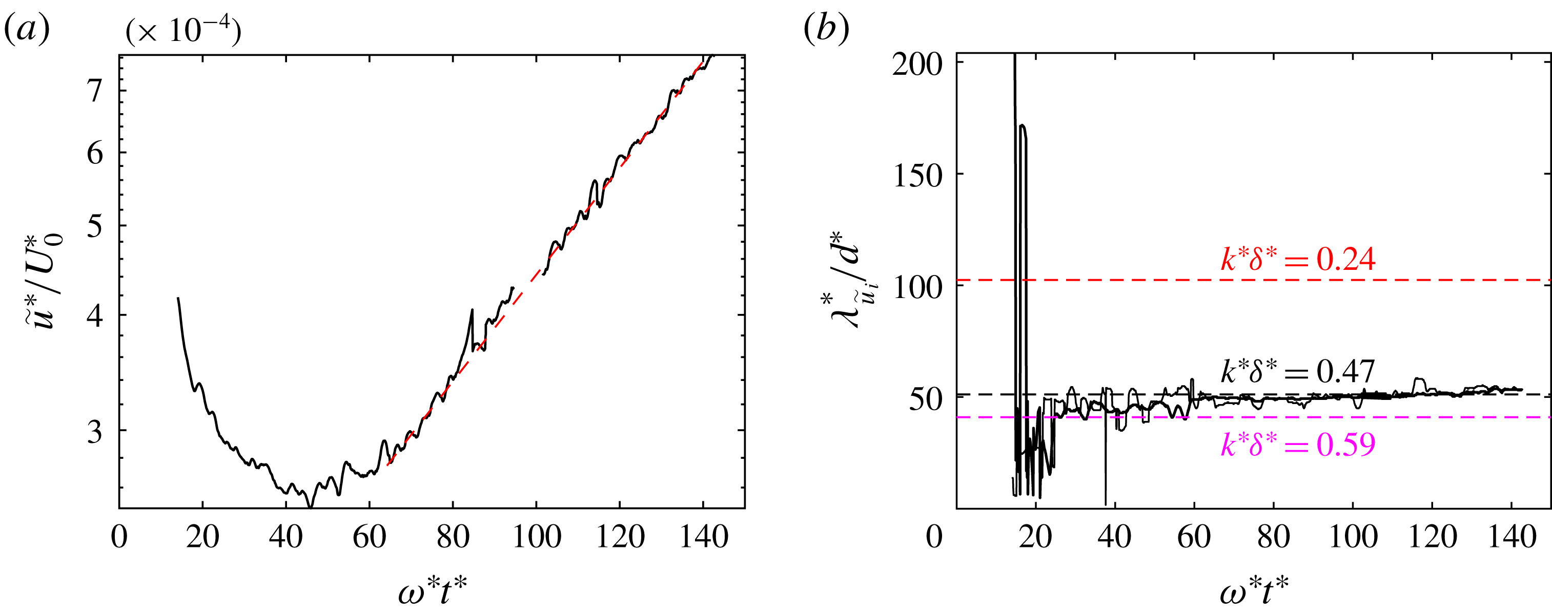Figure 11(a) shows that, in run 1, the value of $\widetilde{u}^{\ast }/U_{0}^{\ast }$ initially decreases, then starts to increase and attains an exponential growth from approximately the tenth oscillation period on, similarly to ripples of wavelength $\unicode[STIX]{x1D706}_{\unicode[STIX]{x1D702}}$ . Moreover, the evolution of the dominant wavelength of the bed profile in figure 7(a) matches closely the evolution of $\unicode[STIX]{x1D706}_{\widetilde{u}_{i}}$ , namely the dominant spatial periodicity of $\widetilde{u}_{1}$ and $\widetilde{u}_{2}$ in the vicinity of the bed, which is shown in figure 11(b). Hence it is evident that the formation of ripples is coupled with the development of recirculating cells. The maximum velocity of the steady streaming is attained in the vicinity of the bed surface and is approximately equal to $1.5\times 10^{-2}U_{0}^{\ast }$ and $0.6\times 10^{-2}U_{0}^{\ast }$ for runs 1 and 2, respectively. Close to the bed, the spatial periodicity and the flow direction of recirculating cells promote the accretion of the ripples characterised by a wavelength equal to $\unicode[STIX]{x1D706}_{\unicode[STIX]{x1D702}}^{\ast }$ . In particular, four pairs of recirculating cells can be observed for run 1 and two pairs for run 2. However, figure 10(a), which refers to run 1, shows that recirculating cells with different periodicity superimpose above the bed and at $x_{2}=13$ only two pairs of recirculating cells can be detected. This is compatible with the evolution of the bed profile described above, in particular with the growth of the mode characterised by $k^{\ast }\unicode[STIX]{x1D6FF}^{\ast }=0.24$ , as shown in figure 6(a). In run 2, contrarily, recirculating cells do not merge far from the bed (cf. figure 10 b).

Figure 11.

(a) Magnitude of the steady streaming averaged over the $x_{1}x_{2}$ -plane,  $\widetilde{u}^{\ast }$ , normalised by $U_{0}^{\ast }$ and plotted versus time with the vertical axis in a logarithmic scale. Note that the small gap in (a) around $\unicode[STIX]{x1D714}t=100$ is due to the loss of some select data. (b) Dominant wavelength of the streamwise (thick line) and wall-normal (thin line) components ( $i=1,2$ ) of the steady streaming velocity at $x_{2}^{\ast }=3.90\unicode[STIX]{x1D6FF}^{\ast }$ . Ripples appear nearly when the growth rate attains an exponential trend with constant rate. Each point of the curve is referred to the time-averaged value computed over the previous period for run 1.

3.2 Dynamics of surficial particles

The process generating the ripples has been described as primarily being driven by the steady secondary flow arising in the boundary layer. In this section, we will evaluate the role that moving particles play in the coupled problem of the bed-surface evolution. Blondeaux (Reference Blondeaux1990) found that the first observable (often called critical) wavenumber of ripples plotted versus $Re_{\unicode[STIX]{x1D6FF}}$ (for fixed values of the other parameters) exhibited discontinuities whenever particles in motion interacted with a different number of recirculating cells. Indeed, the selection of the critical wavenumber is closely related to the ratio between the sediment semi-excursion, $\ell _{s}^{\ast }$ , namely the amplitude of particle oscillations in the streamwise direction, and the wavelength of ripples, $\unicode[STIX]{x1D706}_{\unicode[STIX]{x1D702}}^{\ast }$ . However, $\ell _{s}^{\ast }$ is difficult to measure in the laboratory and Blondeaux (Reference Blondeaux1990) replaced it in his study with the fluid semi-excursion, $\ell _{f}^{\ast }$ , since the two quantities are well correlated. Mazzuoli et al. (Reference Mazzuoli, Kidanemariam, Blondeaux, Vittori and Uhlmann2016), who investigated by DNS the dynamics of a small number of spherical particles in an oscillatory boundary layer, computed the particle semi-excursion and found that it tended to increase almost linearly during the initial oscillation periods, independently of the presence of bottom roughness, as long as particle–particle interactions were relatively unimportant (tests 2–4 of Mazzuoli et al. Reference Mazzuoli, Kidanemariam, Blondeaux, Vittori and Uhlmann2016). The evolution of $\ell _{s}^{\ast }$ was more complex when many particles were considered. Presently, the motion of the top-layer particles, i.e. the spheres at the bed surface, is investigated. Top-layer particles consist of $O(2\times 10^{4})$ spheres. Approximately 12 % of these particles in run 1, and 15 % in run 2, are crest particles, i.e. lay within a distance $d^{\ast }$ from the sphere on top of the bed. The top-layer particles are tracked during each half-period starting from the phase, $\unicode[STIX]{x1D712}$ , when particle motion ceases and then restarts in the opposite direction.

In particular, the particles that at time $t_{j}^{(in)}=\unicode[STIX]{x03C0}(j+\unicode[STIX]{x1D712})$ , $j=0,1,2,\ldots$ are top-layer particles, are tracked for a half-period, $\unicode[STIX]{x1D712}$ being equal to 0.2 for both run 1 and run 2. Crest particles are more exposed to the flow, which gives them higher mobility than those lying in the troughs between the ripples. The trajectories of crest particles obtained for two periods of simulation 1 (when four ripples are present) are marked in figure 12. Figure 12 shows that, at the end of an oscillation, most of the particles recover almost their initial positions except a few particles which can escape a ripple and reach the neighbouring one.

Figure 12.

Trajectories of crest particles during the time interval $126.3<t<138.9$ (two oscillation periods) of simulation 1. The trajectory of one particle is highlighted by a thick red line.

Figure 13.

Probability that top-layer particles located at the instants $t=t_{}^{(in)}$ (for the last five oscillation periods of each run) in a certain position $x_{1}$ experience semi-excursion $\unicode[STIX]{x1D6FC}\equiv |\ell _{s}^{\ast }|>0.5\unicode[STIX]{x1D706}_{\unicode[STIX]{x1D702}}^{\ast }$ (black lines) or time maximum (over each half-period) drag force $\unicode[STIX]{x1D6FC}\equiv \max _{T}\langle F_{1s}^{\ast }\rangle >+0.1F_{ref}^{\ast }$ (red lines) or $\unicode[STIX]{x1D6FC}\equiv \min _{T}\langle F_{1s}^{\ast }\rangle <-0.1F_{ref}^{\ast }$ (blue lines). Dashed lines are equispaced by $\unicode[STIX]{x1D706}_{\unicode[STIX]{x1D702}}^{\ast }/\unicode[STIX]{x1D6FF}^{\ast }$ . The reference drag is defined as $F_{ref}^{\ast }=(1/2)\unicode[STIX]{x1D71A}^{\ast }U_{0}^{\ast }\unicode[STIX]{x1D714}^{\ast }\unicode[STIX]{x1D6FF}^{\ast \,3}$ . Probabilities are computed over the last periods of run 1 (a) and run 2 (b).

Figure 13(a) shows the probability that the semi-excursion, the time-maximum drag force and time-minimum drag force acting on the top-layer particles selected at the instants $t_{j}^{(in)}$ , $j=36,38,\ldots ,41$ , of run 1 and located within $[x_{1}-D,x_{1}+D]$ , exceed the threshold values $0.5\unicode[STIX]{x1D706}_{\unicode[STIX]{x1D702}}^{\ast }$ , $+0.1F_{ref}^{\ast }$ and $-0.1F_{ref}^{\ast }$ , respectively, with $F_{ref}^{\ast }=(1/2)\unicode[STIX]{x1D71A}^{\ast }U_{0}^{\ast }\unicode[STIX]{x1D714}^{\ast }\unicode[STIX]{x1D6FF}^{\ast \,3}$ . Similarly, figure 13(b) refers to the interval between the $t_{54}^{(in)}$ and $t_{59}^{(in)}$ , which is in the final part of simulation 2. For run 1, the values of the particle semi-excursion range between 0 and approximately $0.7\unicode[STIX]{x1D706}_{\unicode[STIX]{x1D702}}^{\ast }$ . Figure 13(a) illustrates that the probability of observing large values of $\ell _{s}^{\ast }$ increases in the vicinity of the ripple crests while it is approximately halved in the troughs. In fact, the drag force acting on crest particles is significantly larger than the drag force acting on other particles, which causes crest particles to move longer (and farther) in the flow direction. Crest particles, at time $t=t_{j}^{(in)}$ , are not aligned along the centre line between the ripple troughs where the streamlines of recirculating cells converge (cf. figure 10), instead, as described in § 3.1, they are mostly piled on the side of each ripple opposite to the flow direction. Therefore, the probability curves related to the drag in figure 13(a) are asymmetric with respect to the centre line of the ripples. Another consequence of the asymmetric shape of the ripple profile is that only a small number of crest particles reach the neighbouring ripple during a half-period, although visualisations show that several crest particles display values of $\ell _{s}^{\ast }$ larger than $0.5\unicode[STIX]{x1D706}_{\unicode[STIX]{x1D702}}^{\ast }$ , because at $t=t_{j}^{(in)}$ most of them are located farther than $0.5\unicode[STIX]{x1D706}_{\unicode[STIX]{x1D702}}^{\ast }$ from the downstream boundary between adjacent ripples. As a result, we observe the ripple crests moving to and fro over the span of $\unicode[STIX]{x1D706}_{\unicode[STIX]{x1D702}}^{\ast }$ . Similar dynamics cannot be detected for run 2 by visual inspection of figure 13(b). In this case, the variability of the drag force acting on top-layer particles is not as pronounced as in run 1 and, as shown in the following, results in the slower evolution of ripples. Also the semi-excursion of top-layer particles is almost independent of the streamwise coordinate and exhibits large values because the average (viscous) drag acts uniformly on the top-layer particles and is relatively strong. The drag coefficient for an isolated particle of run 2, i.e. the drag force normalised by the reference quantity $(1/2)\unicode[STIX]{x1D71A}^{\ast }U_{0}^{\ast \,2}d^{\ast \,2}$ , is approximately two times larger than in run 1). This is shown more clearly in § 3.3 where the sediment flux is related to the shear stress acting on the bed surface.

Figure 14.

Probability density functions of particle semi-excursion (a), drag (b) and velocity (c) of top-layer particles for the 41st and 58th half-periods of run 1 (red lines) and run 2 (black lines), respectively. Drag force is normalised by $F_{ref}^{\ast }=(1/2)\unicode[STIX]{x1D71A}^{\ast }U_{0}^{\ast }\unicode[STIX]{x1D714}^{\ast }\unicode[STIX]{x1D6FF}^{\ast \,3}$ . In the insets, the respective quantities are plotted in semi-logarithmic scale.

Figure 15.

Probability density functions of particle semi-excursion (a), drag (b) and velocity (c) of crest particles for the 41st and 58th half-periods of run 1 (red lines) and run 2 (black lines), respectively. Drag force is normalised by $F_{ref}^{\ast }=(1/2)\unicode[STIX]{x1D71A}^{\ast }U_{0}^{\ast }\unicode[STIX]{x1D714}^{\ast }\unicode[STIX]{x1D6FF}^{\ast \,3}$ . Quantities are normalised by the standard deviation of each sample.

In order to understand why the formation of ripples in run 1 occurs significantly earlier than in run 2, three quantities are presently considered for each top-layer particle throughout the simulations: the particle semi-excursion, the particle velocity and the drag force. Results are first shown in the following for the last simulated half-period, where the differences between the motion of crest particles and of other top-layer particles are pronounced. The probability density function (pdf) of $\ell _{s}$ was computed for the top-layer particles of both run 1 and run 2, which shows that approximately 88 % of top-layer particles set into motion stop within a distance equal to $4d^{\ast }$ from their (previous) rest position (see figure 14 a). Among these sluggish particles there are also crest particles that, however, predominately exhibit large mobility, in particular for run 1. In fact, the core of the pdfs of $\ell _{s}^{\ast }$ , normalised by $\unicode[STIX]{x1D706}_{\unicode[STIX]{x1D702}}^{\ast }$ , is found to be nearly coincident between run 1 and run 2 ( $d^{\ast }$ , $\unicode[STIX]{x1D6FF}^{\ast }$ and $\ell _{f}^{\ast }$ are found not to be relevant scales of the pdf core), while the tail of the curves, which is representative of the most mobile particles, deviates because crest particles behave differently in the two simulations and differently from the other top-layer particles. Such behaviour of crest particles reflects also on the particle velocity and drag, as can be understood from figure 14(b,c). However, by restricting the sample to crest particles and scaling the quantities presently considered by their standard deviation, a fair matching of the pdfs can be obtained, as shown in figure 15. This strategy is not relevant for non-crest particles. The existence of two separated scales suggests that (at least) two types of particle motion coexist: a ‘regular motion’ dominated by viscous forces (slow particles) and an ‘erratic motion’ affected by particle–particle interactions that manifest themselves in random fluctuations of particle forces (crest particles): approximately 50 % of crest particles of run 1 show a wide range of values of $\ell _{s}^{\ast }$ (between $0.10\unicode[STIX]{x1D706}_{\unicode[STIX]{x1D702}}^{\ast }$ and $0.45\unicode[STIX]{x1D706}_{\unicode[STIX]{x1D702}}^{\ast }$ ) with a nearly constant distribution of probability. Instead, the values of $\ell _{s}^{\ast }$ for run 2 are more accumulated around the mean value ( $0.08\unicode[STIX]{x1D706}_{\unicode[STIX]{x1D702}}^{\ast }$ ) than in the other simulation. This is also emphasised by the ratio between the standard deviation, $\unicode[STIX]{x1D70E}_{\ell _{s}}^{\ast }$ , and the mean value, $\langle \ell _{s}^{\ast }\rangle _{s}$ , being equal to 0.88 and 0.67 for runs 1 and 2, respectively. The fact that $\unicode[STIX]{x1D706}_{\unicode[STIX]{x1D702}}^{\ast }$ is not a relevant scale for the semi-excursion of crest particles appears from the values of the statistics shown in table 4. The standard deviation $\unicode[STIX]{x1D70E}_{\ell _{s}}^{\ast }$ computed for run 2 appears significantly smaller than that of run 1 when normalised by $\unicode[STIX]{x1D706}_{\unicode[STIX]{x1D702}}^{\ast }$ . However, the value for each run is approximately 0.03 when normalised by $\ell _{f}^{\ast }$ , which is actually a relevant scale for the semi-excursion of crest particles. The values of $\langle \ell _{s}^{\ast }\rangle _{s}$ for crest particles are equal to $3.6\times 10^{-2}\ell _{f}^{\ast }$ and $5.7\times 10^{-2}\ell _{f}^{\ast }$ for runs 1 and 2, respectively, which are smaller but of the same order (approximately half) as the value obtained by Mazzuoli et al. (Reference Mazzuoli, Kidanemariam, Blondeaux, Vittori and Uhlmann2016) at the end of test no. 6. Actually, in the present case there are factors that contribute to increase the friction between sediments, among them the fact that the bed surface is not macroscopically flat as in the cases investigated by Mazzuoli et al. (Reference Mazzuoli, Kidanemariam, Blondeaux, Vittori and Uhlmann2016) and the number of moving particles (and, consequently, of collisions) is much larger. The maximum value of the particle excursion, $\max _{s}\ell _{s}^{\ast }$ , for run 1 is approximately equal to $0.15\ell _{f}^{\ast }$ and is comparable with those computed from one of the experiments of Rousseaux et al. (Reference Rousseaux, Stegner and Wesfreid2004a ) ( $Re_{\unicode[STIX]{x1D6FF}}\simeq Re_{d}=135$ , $s=2.5$ ) which fell in the range $[0.15,\,0.25]\ell _{f}^{\ast }$ .

Table 4.

Statistics of crest particles.

The discrepancies between the pdfs of the two simulations are not strictly associated with the presence of ripples, as one could be tempted to presume, because the same differences were present since the initial wave cycles when the bedforms were not yet developed. Instead, they can be attributed to the different values of the Keulegan–Carpenter number, $K_{c}$ . In fact, large values of $\ell _{s}$ are associated with large values of $\ell _{f}$ . Moreover, the contribution to the average drag force acting on the particles due to the presence of recirculation cells is smaller in run 2 than in run 1, which leads to more homogeneous distribution of drag over the bed surface. Note that most frequently (in the sense of probability) top-layer particles exhibit a creeping velocity, in particular in the case of run 1 which shows a wider gap between very slow and fast moving particles than run 2 (cf. figure 14 c). Analogous to the process of segregation for polydispersed particulate flows, which occurs because of particle inertia when sediment particles differ in size and/or density, here the growth of bed-surface perturbations is promoted by the non-uniform distribution of drag over top-layer particles (due to the steady streaming) and is faster if the non-homogeneity is more pronounced.

In principle, the mechanism for the origin of the patterns of spheres on the surface of a movable bed is similar to that observed by Mazzuoli et al. (Reference Mazzuoli, Kidanemariam, Blondeaux, Vittori and Uhlmann2016) for beads rolling on a rough plane bottom (tests 4 and 6). In test no. 6 of Mazzuoli et al. (Reference Mazzuoli, Kidanemariam, Blondeaux, Vittori and Uhlmann2016), several movable beads were initially aligned in the direction of the flow oscillations and rapidly spread laterally until, after a few oscillations, they were randomly scattered over the whole bottom. The latter is approximately the initial configuration of the present simulations. The evolution of the values of $\ell _{s}$ , $F_{1s}$ and $u_{1s}$ , averaged over top-layer or crest particles and over each half-cycle, are shown in figure 16. The values of the considered quantities for top-layer particles are approximately constant throughout simulation 2, except for a short initial transient, while a slight monotonic decrease of the three quantities can be noted relative to crest particles. During the transient, both the semi-excursion and the velocity of the top-layer particles decrease because the spheres attain a closely packed configuration. Conversely, crest particles of run 1 manifest increasing mobility since the beginning of the simulation and show an approximately linear growth of the average $\ell _{s}$ and $u_{1s}$ , while drag seems to asymptotically reach a constant value after the initial transient. The increase of mobility of the crest particles is due to the emergence of ripples which push crest particles towards regions of the boundary layer characterised by higher velocity. The effect of the exponential growth of the ripple amplitudes is partly opposed by that of increasing inter-particle collisions. Since the inertia of particles is relatively small in both runs 1 and 2 (as indicated by the large values of $K_{c}$ ), the drag force reaches a limit as it balances the bed friction. Thus, the relative particle velocity, on which the viscous drag depends, remains constant while the absolute particle velocity increases. In fact, as will be clarified in the following section, the viscous drag dominates the other force contributions in the phases when the bed shear stress is at a maximum.

Figure 16.

Statistics of the motion of top-layer (solid lines) and crest (dashed lines) particles: (a) mean particle semi-excursion, (b) maximum velocity, (c) mean time-maximum drag. The values are computed for each half-period of simulation 1 (red lines/squares) and simulation 2 (black lines/circles). Particle semi-excursion for run 1 increases approximately with a linear trend: a similar trend was observed by Mazzuoli et al. (Reference Mazzuoli, Kidanemariam, Blondeaux, Vittori and Uhlmann2016) in their test nos. 2–4.

3.3 Bed shear stress, incipient particle motion and sediment flow rate

The wall-normal dependent total shear stress is a sum of the fluid shear stress $\unicode[STIX]{x1D70F}_{f}^{\ast }$ and the contribution stemming from the fluid–particle interaction $\unicode[STIX]{x1D70F}_{p}^{\ast }$ , viz.

(3.2) $$\begin{eqnarray}\unicode[STIX]{x1D70F}_{tot}^{\ast }=\unicode[STIX]{x1D70F}_{f}^{\ast }+\unicode[STIX]{x1D70F}_{p}^{\ast },\end{eqnarray}$$

where the fluid shear stress (under a turbulent flow condition) is comprised of the viscous and Reynolds shear stress contributions:

(3.3) $$\begin{eqnarray}\unicode[STIX]{x1D70F}_{f}^{\ast }(x_{2}^{\ast })=\unicode[STIX]{x1D71A}^{\ast }\unicode[STIX]{x1D708}^{\ast }{\displaystyle \frac{\unicode[STIX]{x2202}\langle u_{1}^{\ast }\rangle }{\unicode[STIX]{x2202}x_{2}^{\ast }}}(x_{2}^{\ast })-\unicode[STIX]{x1D71A}^{\ast }\langle u_{1}^{\prime \ast }u_{2}^{\prime \ast }\rangle (x_{2}^{\ast }),\end{eqnarray}$$

where the dependence on $t^{\ast }$ is omitted for the sake of clarity. Although the total shear stress in the presence of two-dimensional ripples is homogeneous in the spanwise direction, relatively small fluctuations about $\unicode[STIX]{x1D70F}_{tot}^{\ast }$ can be observed in the streamwise direction when the rolling-grain ripples form. Thus, $\unicode[STIX]{x1D70F}_{tot}^{\ast }$ is the average total shear stress acting on the bed. It is expected that, in the present configuration, the Reynolds shear stress makes a negligible contribution as the flow is essentially laminar. In the context of the immersed boundary method, the stress exerted by the particles is given by

(3.4) $$\begin{eqnarray}\unicode[STIX]{x1D70F}_{p}^{\ast }(x_{2}^{\ast })=\unicode[STIX]{x1D71A}^{\ast }\int _{x_{2}^{\ast }}^{L_{x_{2}}^{\ast }}\langle f_{1}^{\ast }\rangle \,\text{d}x_{2}^{\ast },\end{eqnarray}$$

where $f_{1}^{\ast }$ is the streamwise component of the immersed boundary method volume forcing exerted on the fluid, transferred to the Eulerian grid (cf. § 2). In a stationary channel flow scenario, the total shear stress varies linearly in the wall-normal direction with a slope equal to the value of the imposed driving pressure gradient. 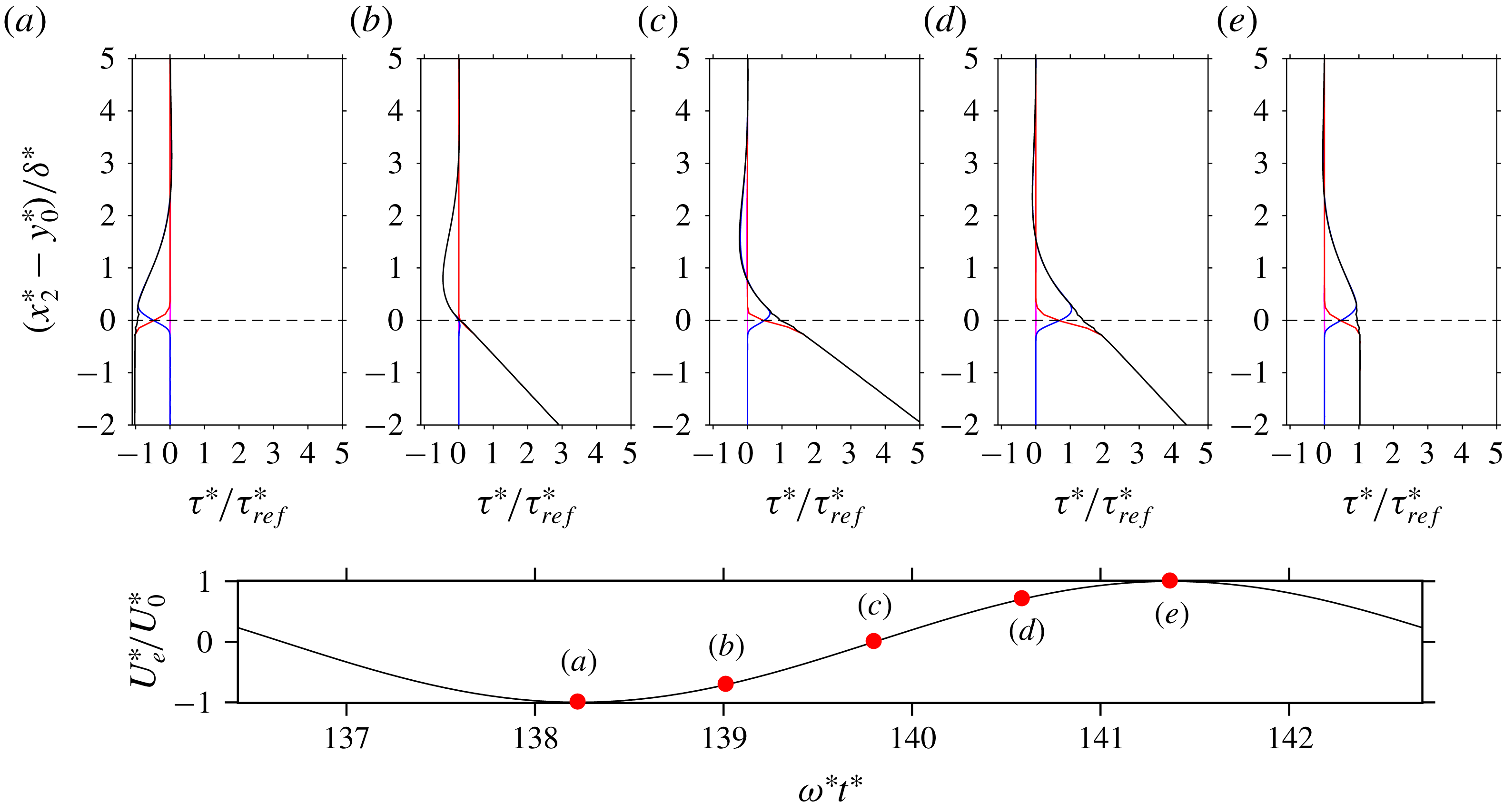In the present OBL configuration however, as a result of the non-stationarity, $\unicode[STIX]{x1D70F}_{tot}^{\ast }$ responds to the pressure gradient with a complex nonlinear behaviour. Figure 17 shows sample wall-normal profiles of the different contributions to the total shear stress, non-dimensionalised by $\unicode[STIX]{x1D70F}_{ref}^{\ast }=(1/2)\unicode[STIX]{x1D71A}^{\ast }U_{0}^{\ast }\unicode[STIX]{x1D714}^{\ast }\unicode[STIX]{x1D6FF}^{\ast }$ , at different time instants. As is expected, the contribution from the Reynolds shear stress is negligibly small across the entire wall-normal interval which is a further indication that the flow has not separated behind the ripple crests. In the clear fluid region, that is, in the region which is essentially devoid of sediment particles, only the fluid viscous shear stress contributes to $\unicode[STIX]{x1D70F}_{tot}$ . On the other hand, deep inside the sediment bed sufficiently below the fluid–bed interface, $\unicode[STIX]{x1D70F}_{f}$ vanishes and $\unicode[STIX]{x1D70F}_{tot}$ is entirely comprised of the stress exerted by the sediment particles. It is worth noting that, in this region, $\unicode[STIX]{x1D70F}_{tot}$ exhibits a linear variation with a slope equal to the imposed pressure gradient. This means that the particle shear resistance, which is proportional to the submerged weight of sediment bed, is instantaneously in equilibrium with the oscillating driving force (neglecting the small particle velocities in this region). In between these two regions, there exists a third ‘active-layer’ region, hereafter referred to as the mobile layer, where both $\unicode[STIX]{x1D70F}_{f}$ and $\unicode[STIX]{x1D70F}_{p}$ contribute to the total shear stress and where the particle erosion–deposition processes take place. Although there is no clear demarcation of these regions, it is observed that the thickness of the mobile layer varies depending on different phases of the oscillation period.

Figure 17.

Sample wall-normal profiles of the fluid viscous shear stress (blue line), Reynolds shear stress (magenta line), stress stemming from the fluid–particle interaction (red line) as well as the total shear stress $\unicode[STIX]{x1D70F}_{tot}$ (black line). The profiles correspond to selected times which are indicated in (f). Data correspond to run 1.

For modelling purposes, it is common practice to relate the non-dimensional boundary shear stress $\unicode[STIX]{x1D70F}_{b}^{\ast }=\unicode[STIX]{x1D70F}_{tot}^{\ast }(x_{2}^{\ast }=y_{0}^{\ast })$ , i.e. the Shields number

(3.5) $$\begin{eqnarray}\unicode[STIX]{x1D703}=\frac{\unicode[STIX]{x1D70F}_{b}^{\ast }}{(\unicode[STIX]{x1D71A}_{s}^{\ast }-\unicode[STIX]{x1D71A}^{\ast })g^{\ast }d^{\ast }}\end{eqnarray}$$

to the sediment flow rate. The value of $y_{0}^{\ast }$ is chosen as the distance from the bottom at which the average particle volume fraction $\langle \unicode[STIX]{x1D719}_{s}\rangle$ reaches 0.1. The instantaneous volumetric flow rate of the particle phase (per unit span), $q_{s}^{\ast }$ , is given by

(3.6) $$\begin{eqnarray}q_{s}^{\ast }(t^{\ast })=\frac{\unicode[STIX]{x03C0}d^{\ast \,3}}{6\,L_{x_{1}}^{\ast }L_{x_{3}}^{\ast }}\mathop{\sum }_{l=1}^{N_{p}}u_{1s}^{\ast (l)}(t^{\ast }),\end{eqnarray}$$

where $u_{1s}^{\ast (l)}(t^{\ast })$ is the streamwise component of the velocity of the $l$ th mobile particle at time $t^{\ast }$ . Since spherical particles do not gear to each other and can slide more easily than sand grains, many particles experience non-zero velocities, even if they are located below the bed surface. Thus, in order to exclude all particles which do not contribute to the shear-induced particle flux, a streamwise velocity threshold is set at 1 % of the gravitational velocity of the particles, $v_{s}^{\ast }$ (similar results are obtained even considering the threshold at a small percentage of $\unicode[STIX]{x1D714}^{\ast }\unicode[STIX]{x1D6FF}^{\ast }$ ). The particles selected with such a criterion approximately coincide with those constituting the mobile layer (cf. figure 18).

Figure 18.

The streamwise component of the particle velocity is plotted as a function of the wall-normal coordinate of run 1. Shaded by grey dots are the velocity of each particle at the instants $t=36.75\unicode[STIX]{x03C0}$ (I), $t=37.00\unicode[STIX]{x03C0}$ (II) and $t=37.25\unicode[STIX]{x03C0}$ (III) (phases are indicated in the inset), while thin solid, thick solid and dashed lines indicate the respective (binned) average values.

Figure 19.

Instantaneous dimensionless particle flow rate, normalised by the inertial scaling $d^{\ast }v_{s}^{\ast }$ , as a function of the Shields number $\unicode[STIX]{x1D703}$ during the last four cycles of the simulation interval. Run 1 (red line); run 2 (black line). The dashed line represents the the Meyer-Peter & Müller formula (Wong & Parker Reference Wong and Parker2006) for steady turbulent flow conditions $q_{s}=4.93(\unicode[STIX]{x1D703}-\unicode[STIX]{x1D703}_{c})^{1.6}$ . The symbols ▵, ○, ▫ indicate phases $t=(1/8)\unicode[STIX]{x03C0}$ , $t=(9/32)\unicode[STIX]{x03C0}$ and $t=(6/8)\unicode[STIX]{x03C0}$ , while small circle–cross and circle–plus symbols mark the instants at which the velocity far from the bottom vanishes ( $t=(4/8)\unicode[STIX]{x03C0}$ ) and reaches $U_{0}^{\ast }$ ( $t=\unicode[STIX]{x03C0}$ ), respectively. Grey circles indicate the experimental observations of Gilbert and Meyer-Peter (Nielsen Reference Nielsen1992).

Figure 19 shows the absolute value of the particle flow rate, normalised by $d^{\ast }v_{s}^{\ast }$ , as a function of the absolute value of the Shields number for the last four periods of run 1 and run 2. The arrows indicate the time development along the loop swept in a half-period. Following the loop, the particle flow rate exhibits a minimum in the early deceleration phase (see phase $t\simeq (1/8)\unicode[STIX]{x03C0}$ in figure 19). Then, while the free-stream velocity is still decelerating and the Shields number decreasing, the particle flow rate increases under the action of the imposed driving pressure gradient (between phases $t\simeq (1/8)\unicode[STIX]{x03C0}$ and $t\simeq (5/8)\unicode[STIX]{x03C0}$ in figure 19). Subsequently, the next acceleration phase starts and the Shields number rises. Finally, approximately at the phase $(3/4)\unicode[STIX]{x03C0}$ (i.e. $(1/4)\unicode[STIX]{x03C0}$ after the flow reversal), both the Shields number (i.e. the boundary shear stress) and the sediment flow rate are maximum. It can be noted that, except for two or three instants, each value of $|\unicode[STIX]{x1D703}|$ corresponds to two values of the dimensionless sediment flow rate. It is therefore clear, by comparing the diagrams of figure 19 obtained for the present runs with the experimental measurements of Gilbert and Meyer-Peter (grey symbols, Nielsen Reference Nielsen1992) and with the Meyer-Peter & Müller formula (dashed line, Wong & Parker Reference Wong and Parker2006) obtained for stationary channel flows, that the effects of the flow unsteadiness impact strongly on the motion of particles and should be taken into account in the models of sediment transport. Indeed, during the flow reversal, which is characterised by large values of the forcing pressure gradient and relatively small values of the bed shear stress, the sediment flow rate is not negligible. Hence, coarse prediction errors could be avoided by relating the sediment flow rate to a combination of the Shields number and some dimensionless expression of the pressure gradient such as the instantaneous Sleath parameter (Foster et al. Reference Foster, Bowen, Holman and Natoo2006; Frank et al. Reference Frank, Foster, Sou, Calantoni and Chou2015), defined as:

(3.7) $$\begin{eqnarray}{\mathcal{S}}=-{\displaystyle \frac{d^{\ast }}{\unicode[STIX]{x1D71A}^{\ast }v_{s}^{\ast 2}}}{\displaystyle \frac{\text{d}p_{f}^{\ast }}{\text{d}x_{1}^{\ast }}}={\displaystyle \frac{\unicode[STIX]{x1D713}}{K_{c}}}\sin (t),\end{eqnarray}$$

where the expression (2.1) was substituted in the second equality. Since the values of the Keulegan–Carpenter number, $K_{c}$ , are large in both of the present simulations, the contribution of the viscous drag is expected to dominate over that induced on the spheres by the pressure gradient. Besides the direct contribution to the particle force, the pressure gradient also causes the acceleration of the interstitial fluid which, due to its small inertia, responds much earlier than the clear fluid above the bed. Thus, such viscous pore flow develops and can mobilise the sediment particles much earlier than the phase at which the bed shear stress becomes appreciable. Even though the velocity of the particles set into motion during the flow reversal is small, the thickness of the mobile layer is relatively large in these phases because the pressure gradient acts uniformly over the entire bed. Finally, as the values of $|\unicode[STIX]{x1D703}|$ become large, crest particles, which are more exposed to the flow in the boundary layer and exhibit values of streamwise (particle) velocity of order $O(0.1)U_{0}^{\ast }$ , mostly contribute to the sediment flow rate.

Figure 19 also shows that, at corresponding phases, the Shields number and, therefore, the sediment flow rate normalised by $d^{\ast }v_{s}^{\ast }$ , are larger in run 2 than in run 1. To understand such difference it is useful to compare the Shields number to that we would observe in absence of sediments, i.e. in a Stokes boundary layer:

(3.8) $$\begin{eqnarray}\unicode[STIX]{x1D703}_{(St)}={\displaystyle \frac{\unicode[STIX]{x1D713}}{Re_{\unicode[STIX]{x1D6FF}}}}[\sin (\unicode[STIX]{x1D714}^{\ast }t^{\ast })-\cos (\unicode[STIX]{x1D714}^{\ast }t^{\ast })].\end{eqnarray}$$

Figure 20 shows that, scaling the Shields number by the maximum value of $\unicode[STIX]{x1D703}_{(St)}$ , the resulting curves of runs 1 and $2$ almost overlap and the amplitude of the oscillations is nearly equal to unity, because the bed shear stress approaches that of a Stokes boundary layer in both runs. Consequently, the quantity $(1/2)\unicode[STIX]{x1D71A}^{\ast }U_{0}^{\ast }\unicode[STIX]{x1D714}^{\ast }\unicode[STIX]{x1D6FF}^{\ast }$ is a relevant scale for the bed shear stress. Hence, for a given value of $\unicode[STIX]{x1D713}$ , by increasing the value of $Re_{\unicode[STIX]{x1D6FF}}^{\ast }$ the Shields parameter decreases (as in the present case) until turbulence appears and further modes of sediment transport occur (e.g. saltation). Moreover, it can be noted that the maximum value $\max (\unicode[STIX]{x1D703}_{(St)})=\sqrt{2}\unicode[STIX]{x1D713}/Re_{\unicode[STIX]{x1D6FF}}$ equals the maximum value of the Sleath number, i.e. approximately the maximum effect of the imposed pressure gradient on an isolated particle, $\max ({\mathcal{S}})=(\unicode[STIX]{x1D713}/K_{c})=2(d^{\ast }/\unicode[STIX]{x1D6FF}^{\ast })\unicode[STIX]{x1D713}/Re_{\unicode[STIX]{x1D6FF}}$ , if $d^{\ast }/\unicode[STIX]{x1D6FF}^{\ast }\sim 0.7$ . Therefore, even though the maximum shear stress and the maximum imposed pressure gradient are reached at different phases of the oscillation period, in the present cases (and in most of the experiments of Blondeaux et al. Reference Blondeaux, Sleath and Vittori1988) viscous effects prevail. It can be useful to point out that typically, in the field, the ratio $d^{\ast }/\unicode[STIX]{x1D6FF}^{\ast }$ does not significantly vary with respect to the other parameters (e.g. for $0.2~\text{mm}<d^{\ast }<1~\text{mm}$ and $T\sim 10~\text{s}$ , $0.1<d^{\ast }/\unicode[STIX]{x1D6FF}^{\ast }<0.6$ ), thus the ratio $\unicode[STIX]{x1D713}/Re_{\unicode[STIX]{x1D6FF}}$ can be practically used as the only parameter driving the sediment flow rate (as long as the flow is not turbulent). It can be inferred from the present results that the growth rate of ripples is related to the maximum sediment flow rate. In particular, the growth rate of ripples increases if the maximum bed shear stress is not much larger than the critical value of incipient sediment motion, sediments being more sensitive to the effect of the steady streaming. Consequently, if the ratio $\unicode[STIX]{x1D713}/Re_{\unicode[STIX]{x1D6FF}}$ is close to $\unicode[STIX]{x1D703}_{cr}/\sqrt{2}\sim 0.035$ ripples form more rapidly. In fact, for runs 1 and 2, $\unicode[STIX]{x1D713}/Re_{\unicode[STIX]{x1D6FF}}$ is equal to 0.076 and 0.110, respectively, and ripples form much more slowly in case 2. The relevance of $\unicode[STIX]{x1D713}/Re_{\unicode[STIX]{x1D6FF}}$ for the prediction of ripple genesis was also emphasised by Blondeaux (Reference Blondeaux1990) (see figure 11) because it is related to the ratio $\langle \ell _{s}^{\ast }\rangle _{s}/\unicode[STIX]{x1D706}_{\unicode[STIX]{x1D702}}^{\ast }$ . In particular, the dimensionless parameter used by Blondeaux (Reference Blondeaux1990) and by other authors before was $d^{\ast }/(s-1)g^{\ast }T^{\ast 2}$ which is equal to $(1/\unicode[STIX]{x03C0}^{2})(\unicode[STIX]{x1D713}/Re_{\unicode[STIX]{x1D6FF}}^{2})(d^{\ast 2}/\unicode[STIX]{x1D6FF}^{\ast 2})$ and was empirically found to be controlling the ripple wavelength.

Figure 20.

Evolution of the Shields number for run 1 (red line) and run 2 (black line) during the last simulated periods. In (b) the Shields number is normalised by the maximum Shields number attained in the absence of particles, i.e. in a Stokes boundary layer.