
1. Introduction
The ‘coffee-ring effect’ takes its name from the ring-like deposits left behind on a surface after a spilled droplet of coffee has evaporated into the surrounding air. As uncovered by the seminal work of Deegan et al. (Reference Deegan, Bakajin, Dupont, Huber, Nagel and Witten1997, Reference Deegan, Bakajin, Dupont, Huber, Nagel and Witten2000) for an axisymmetric droplet, surface inhomogeneities tend to pin the circular contact line of the droplet so that, to replenish fluid lost during evaporation, an outward radial capillary flow develops inside the droplet; this flow carries solute with it, leading to a build up of solute at the droplet edge. This radial flow may be enhanced by a singularity in the evaporative flux that occurs near the contact line when evaporation is diffusion-dominated (Deegan et al. Reference Deegan, Bakajin, Dupont, Huber, Nagel and Witten2000), but occurs even for uniform evaporation (Masoud & Felske Reference Masoud and Felske2009; Kang et al. Reference Kang, Vandadi, Felske and Masoud2016). Eventually, the solute becomes sufficiently concentrated near the contact line that particle concentration effects such as increased local suspension viscosity (Kaplan & Mahadevan Reference Kaplan and Mahadevan2015) and jamming (Popov Reference Popov2005) become relevant, forming the coffee ring that remains once all liquid has evaporated.
This behaviour is not limited to coffee, but is ubiquitous whenever a liquid droplet containing a solute is left to evaporate. It is vital to understand how to control the effect in many different biological, industrial and engineering settings (Anyfantakis & Baigl Reference Anyfantakis and Baigl2015). There are a number of different mechanisms that can be employed to control the shape of the deposit (Mampallil & Eral Reference Mampallil and Eral2018). A common approach to inhibit coffee-ring formation is to interfere with the pinning of the contact line by, for example, employing superhydrophobic substrates (see, for example, Cui et al. Reference Cui, Zhang, Zhang, Li, Wang, Gao, Wang, Zhu, Yu and Yang2012; Dicuangco et al. Reference Dicuangco, Dash, Weibel and Garimella2014), using electrowetting to encourage contact line slippage (for example, Li & Mugele Reference Li and Mugele2008), or utilizing an oil-coated substrate (for example, Li et al. Reference Li, Diddens, Segers, Wijshoff, Versluis and Lohse2020). Alternatively, one can encourage physical effects that counter the outward capillary flow, such as Marangoni effects (see, for example, Hu & Larson Reference Hu and Larson2006; Ristenpart et al. Reference Ristenpart, Kim, Domingues, Wan and Stone2007; Li et al. Reference Li, Lv, Li, Quéré and Zheng2015) or exploiting electrostatic or electro-osmotic controls (for example, Wray et al. Reference Wray, Papageorgiou, Craster, Sefiane and Matar2014; Kim et al. Reference Kim, Kang, Lee, Kang and Yoon2006). One can also introduce other liquids to the drop: the evaporation of binary droplets is a more complex phenomenon, exhibiting several different flow stages depending on, for example, the relative volatility of the liquid components, which can lead to an interesting variety of deposit patterns (see, for example, Kim et al. Reference Kim, Boulogne, Um, Jacobi, Button and Stone2016; Zhong & Duan Reference Zhong and Duan2016; Li et al. Reference Li, Lv, Diddens, Tan, Wijshoff, Versluis and Lohse2018; Pahlavan et al. Reference Pahlavan, Yang, Bain and Stone2021, and the references therein).
In this paper, we consider the role of droplet geometry on the coffee-ring effect. The geometry of a sessile drop can be controlled readily in a laboratory setting, which makes it a valuable tool for potential control of the deposition pattern. For example, a droplet on a sloped surface will be perturbed away from a spherical cap profile by gravity, which leads to a change in the angular dependence of the evaporative flux (Timm et al. Reference Timm, Dehdashti, Darban and Masoud2019; Tredenick et al. Reference Tredenick, Forster, Pethiyagoda, van Leeuwen and McCue2021). The droplet contact set can also be manipulated by machining or treating the substrate in such a way that pinning at particular points is promoted, altering the shape of the deposit (He et al. Reference He, Yang, Xue, Sun and Cao2017; Sáenz et al. Reference Sáenz, Wray, Che, Matar, Valluri, Kim and Sefiane2017; Kubyshkina et al. Reference Kubyshkina, Orejon, Dover and Sefiane2020).
Once asymmetry is introduced, there is no longer uniformity in the coffee-ring profile. Deegan et al. (Reference Deegan, Bakajin, Dupont, Huber, Nagel and Witten1997) noted that coffee stains tended to be darker near more curved regions of the contact line of a drying droplet, stating that the (diffusive) evaporative flux is larger in these regions, which in turn drives a stronger capillary flow. Sáenz et al. (Reference Sáenz, Wray, Che, Matar, Valluri, Kim and Sefiane2017) performed a range of experiments and simulations of different shaped contact sets, suggesting that in addition to the contact line curvature, the mean curvature of the droplet free surface plays an integral role in the evaporation rate.
While an increased evaporation rate near highly curved parts of the contact line certainly contributes to an enhanced transport of solute mass into these regions, it is not a necessary requirement. Just as the radial flow that generates a coffee ring persists for a uniform evaporation rate in an axisymmetric droplet, the effects of contact line curvature can also be seen for a uniform evaporative flux. In particular, Freed-Brown (Reference Freed-Brown2015) conducted a numerical investigation of the mass flux of solute into the contact line for a wide range of different droplet profiles evaporating under a uniform evaporative flux. Even in the absence of spatially-varying evaporative flux, the liquid velocity is still enhanced towards the highly curved parts of the boundary, so there is a greater mass flux of solute to this part of the boundary, again acting to strengthen the coffee-ring effect.
In the present work, we extend our recent analysis (Moore, Vella & Oliver Reference Moore, Vella and Oliver2021) to gain an understanding of the early stages of coffee-ring formation for arbitrary contact line geometries. In the model of Deegan et al. (Reference Deegan, Bakajin, Dupont, Huber, Nagel and Witten1997, Reference Deegan, Bakajin, Dupont, Huber, Nagel and Witten2000), the solute is sufficiently dilute in the fluid that it is advected radially outwards by the capillary flow, with all of the solute concentrated in an infinitesimally small ring at the contact line once the liquid has evaporated completely. Naturally, real coffee rings have finite dimensions, and the Deegan model can be adapted to incorporate the effects of finite solute concentration (see, for example, Popov Reference Popov2005; Kaplan & Mahadevan Reference Kaplan and Mahadevan2015). However, an important aspect of the dilute problem that is missing in the Deegan model is the effect of solute diffusion, which resists the development of large spatial gradients induced by particle advection close to the contact line. For a thin axisymmetric droplet, Moore et al. (Reference Moore, Vella and Oliver2021) performed an asymptotic analysis in the physically relevant limit of small capillary number and large solutal Péclet number to show that by including the effects of diffusion, the characteristic narrow peaked coffee ring develops even in the early stages of evaporation, for which the solute remains dilute. The local form of the coffee ring was shown to collapse onto a universal gamma distribution profile, and predictions were made about characteristics of this nascent coffee ring, such as its height and thickness under different evaporation laws. Critically, the results of the asymptotic analysis were used to determine when the assumption of a dilute solute breaks down; beyond this regime, it is necessary to incorporate a model for finite concentration effects. In particular, the window over which the dilute regime is valid was found to depend strongly on whether evaporation is kinetic- or diffusion-limited.
Droplet axisymmetry greatly simplifies both the capillary flow and the solute transport problem so that significant analytical progress is possible in the asymptotic analysis. Moore et al. (Reference Moore, Vella and Oliver2021) exploited this relative simplicity to construct consistent composite predictions for the solute mass profile. However, once axisymmetry is broken, the problem becomes much more challenging analytically and this approach is no longer feasible.
Our aim in the present analysis is thus threefold. First, we present an alternative asymptotic approach utilizing an integrated mass variable and an intermediate region that allows us to construct a composite solution for the solute concentration for an arbitrary, smooth, droplet contact set. We demonstrate the methodology in detail for a kinetic evaporation model – in which the evaporative flux is constant – as well as for a diffusive evaporation model for which the evaporative flux is singular at the contact line. These models correspond to two limits of the vapour confinement (high and low, respectively), and the asymptotic results allow us to derive a similarity profile for the nascent coffee ring in these cases.
Second, we use the asymptotic results to investigate the relative importance of droplet asymmetry and heterogeneity in the evaporative flux on mass flux into the contact line and the nascent coffee-ring structure by considering the particular example of a droplet with an elliptical contact set. When the evaporation is dominated by diffusion, we corroborate the findings of Sáenz et al. (Reference Sáenz, Wray, Che, Matar, Valluri, Kim and Sefiane2017) by demonstrating that there is an increased mass flux of solute into the contact line along the highly curved semi-major axis of the ellipse compared to an axisymmetric droplet of the same volume and contact line length. However, when considering the constant evaporative flux model, we demonstrate that asymmetry in the droplet profile alone results in the same behaviour, consistent with the numerical results of Freed-Brown (Reference Freed-Brown2015). In both cases, we derive analytical expressions for the nascent coffee-ring profile, as well as key characteristics such as its height and width.
Importantly, we also demonstrate that the increased mass flux does not necessarily translate to a higher coffee-ring peak. Indeed, for a diffusively-evaporating droplet, we show that as the eccentricity of the elliptical contact set is changed but the droplet volume and perimeter are fixed, the coffee-ring profile along the semi-major axis undergoes a transition from a thinner, higher coffee ring (compared to the corresponding axisymmetric droplet) to a lower, shallower coffee ring. On the other hand, for a uniformly evaporating droplet, the coffee-ring peak along the semi-major axis is always larger than that for the equivalent circular droplet, although there is still a transition from a narrower to a thicker ring.
Finally, we are able to show that this enhanced coffee-ring effect leads to a reduction in the applicability of the dilute model along the semi-major axis, although the duration of applicability is correspondingly longer along the semi-minor axis, where the coffee-ring effect is weaker.
The content of the paper is as follows. In § 2, we present a mathematical model for the evaporation of a thin droplet with an arbitrary, smooth contact set containing a dilute solute, describing the liquid flow in the droplet in the surface-tension-dominated limit. We then consider the solute transport problem in detail in § 3, focusing on the physically relevant regime in which advection dominates diffusion except in a boundary layer close to the pinned contact line. We use our asymptotic analysis to investigate the evaporation of droplets with an elliptical contact set in § 4, uncovering the role played by droplet geometry in the formation of the nascent coffee ring, as well as exploring the limitations of the dilute model. We conclude by summarizing our results in § 5, as well as discussing possible applications and extensions of the model.
2. Formulation of the mathematical model
A droplet of liquid of volume  $V^{*}$ lies on a planar substrate at
 $z^{*} = 0$, where we take Cartesian axes
 $(x^{*},y^{*},z^{*})$ centred with origin inside the droplet contact set
 $\varOmega ^{*}$. Here and hereafter, an asterisk denotes a dimensional variable. The droplet contact line is denoted by
 $\partial \varOmega ^{*}$, and throughout our analysis, we will assume that it is pinned; this is a reasonable assumption for the majority of the drying time (see, for example, Deegan et al. Reference Deegan, Bakajin, Dupont, Huber, Nagel and Witten2000; Kajiya, Kaneko & Doi Reference Kajiya, Kaneko and Doi2008; Orejon, Sefiane & Shanahan Reference Orejon, Sefiane and Shanahan2011). We will assume that the droplet is thin so that if we denote a typical size of the contact set by
 $R^{*}$, we have
 $\delta = V^{*}/R^{*3}\ll 1$. We note that in our analysis of elliptical contact sets in § 4, we will take
 $R^{*}$ to be the length of the semi-minor axis, so that when comparing droplets of the same initial volume and contact line perimeter,
 $\delta$ will necessarily change.
The incompressible Newtonian liquid has constant density  $\rho ^{*}$ and viscosity
 $\mu ^{*}$, while the air–liquid surface traction is taken to be due to a constant surface tension with coefficient denoted by
 $\sigma ^{*}$. We will assume that the droplet is sufficiently small that the effects of gravity are negligible, i.e. we assume that the Bond number
 $Bo = \rho ^{*} g^{*} R^{*2}/\sigma ^{*}$ is small, where
 $g^{*}$ is the gravitational acceleration. The liquid lies in the region
 $0< z^{*}< h^{*}(x^{*},y^{*},t^{*})$ for
 $(x^{*},y^{*})\in \varOmega ^{*}$, where the air–liquid interface lies at
 $z^{*} = h^{*}(x^{*},y^{*},t^{*})$. The liquid velocity and pressure are denoted by
 $\boldsymbol {u}^{*}(x^{*},y^{*},z^{*},t^{*})$ and
 $p^{*}(x^{*},y^{*},z^{*},t^{*})$, respectively.
The liquid contains a non-volatile solute of concentration  $\phi ^{*}(x^{*},y^{*},z^{*},t^{*})$, which is initially uniformly distributed, with concentration
 $\phi _{{init}}^{*}$. One of our key assumptions is that the solute is sufficiently dilute that the flow within the drop is unaffected by its presence. Under the dilute assumption, we can decouple the flow in the liquid drop from the solute transport. One of our aims is to test the validity of this assumption local to the pinned contact line, where the solute concentration increases as a result of the growth of the nascent coffee ring.
The droplet evaporates into the surrounding air, which induces a flux of vapour  $E^{*}$ at the droplet surface. The evaporative process is assumed to be quasi-steady, which is reasonable for a wide range of different liquid–substrate combinations (Hu & Larson Reference Hu and Larson2002). The evaporative flux
 $E^{*}$, combined with the geometry of the droplet, drives a liquid flow of typical size
 $U^{*} = \mathcal {E}^{*}/\delta \rho ^{*}$ towards the pinned contact line, where
 $\mathcal {E}^{*}$ is a typical size of the evaporative flux, which depends upon the evaporation model chosen (see, for example, Murisic & Kondic Reference Murisic and Kondic2011).
2.1. Dimensionless model
The derivation of the model for the liquid flow and solute transfer is a direct extension of the axisymmetric case presented in Moore et al. (Reference Moore, Vella and Oliver2021), so here we will present the model directly in dimensionless form in the interests of brevity. Exploiting the thinness of the droplet and assuming that the flow is sufficiently slow to be dominated by viscosity, the pertinent scalings are
 \begin{equation} (x^{*},y^{*}) = R^{*}(x,y), \quad z^{*} = \begin{cases} \delta R^{*}\hat{z}, & \text{in the droplet},\\ R^{*}z, & \text{in the air}, \end{cases} \quad t^{*} = \frac{R^{*}t_{f}}{U^{*}}t, \end{equation}
and
 \begin{equation} \left. \begin{gathered} h^{*} = \delta R^{*}h, \quad \boldsymbol{u}^{*} = (u^{*},v^{*},w^{*}) = U^{*}(u,v,\delta w), \\ p^{*} = p_{{atm}}^{*} + \frac{\mu^{*}U^{*}}{\delta^{2}R^{*}}\,p, \quad E^{*} = \delta \rho^{*}U^{*}E, \quad \phi^{*} = \phi_{{init}}^{*}\phi, \end{gathered} \right\} \end{equation}
where  $p_{{atm}}^{*}$ is the atmospheric pressure, and the (dimensionless) dryout time of the droplet is defined by
 \begin{equation} t_{f} = \left(\iint_{\varOmega}E\,{\rm d}S\right)^{{-}1}. \end{equation}
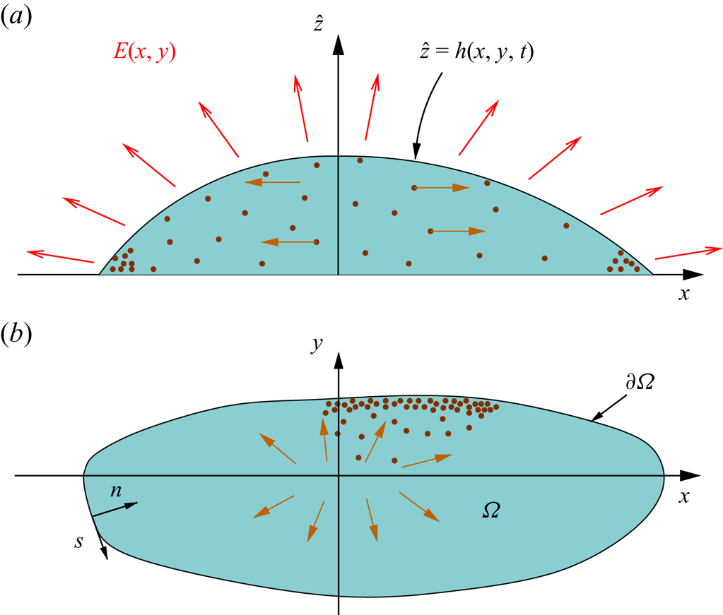
Note that we have scaled time such that the dimensionless lifetime of the droplet is  $0< t<1$, to simplify the analysis going forward. The dimensionless droplet configuration is shown in figure 1.
(a) Side-on and (b) top-down views of a partially-wetting liquid droplet with dimensionless contact set  $\varOmega$ and pinned contact line
 $\partial \varOmega$ in the plane
 $\hat {z} = 0$ of the rigid impermeable substrate. The droplet evaporates into the surrounding air with flux
 $E(x,y)$ as indicated by the red arrows. The orange arrows indicate the evaporation-induced solute velocity. The liquid–air interface is denoted by
 $\hat {z} = h(x,y,t)$. The local orthogonal curvilinear coordinate system
 $(s,n)$ embedded in the contact line described in § 2.3 can be seen in (b).

2.1.1. Flow model
As described in, for example, Deegan et al. (Reference Deegan, Bakajin, Dupont, Huber, Nagel and Witten2000), Freed-Brown (Reference Freed-Brown2015) and Moore et al. (Reference Moore, Vella and Oliver2021), since the droplet is assumed to be thin, to leading order the fluid flows within the drop according to the lubrication equations given by
 \begin{equation} \frac{1}{t_{f}}\,\frac{\partial h}{\partial t} + \boldsymbol{\nabla}\boldsymbol{\cdot}\left(h\bar{\boldsymbol{u}}\right) ={-} E, \quad \bar{\boldsymbol{u}} ={-}\frac{h^{2}}{3}\,\boldsymbol{\nabla} p, \quad p ={-}\frac{1}{{{Ca}}}\,\nabla^{2}h, \end{equation}
for  $(x,y)\in \varOmega$,
 $0< t<1$, where
 $\boldsymbol {\nabla } = (\partial /\partial x,\partial /\partial y)^{\textrm {T}}$. Here,
 $\bar {\boldsymbol {u}}(x,y,t)$ is the leading-order depth-averaged velocity of the droplet, the leading-order pressure
 $p(x,y,t)$ is independent of
 $\hat {z}$, and the capillary number is
 \begin{equation} {{Ca}} = \frac{U^{*}\mu^{*}}{\sigma^{*}\delta^{3}}. \end{equation}
Equations (2.4) are supplemented by boundary conditions that require the droplet thickness to vanish and there to be no flux of liquid through the pinned contact line, so that
 \begin{equation} h = h\bar{\boldsymbol{u}}\boldsymbol{\cdot}\boldsymbol{n} = 0 \quad \mathrm{on} \ \partial\varOmega, \end{equation}
where  $\boldsymbol {n}$ is the outward pointing unit normal to
 $\partial \varOmega$, while we must prescribe the initial droplet profile,
 $h_{0}$ say, so that
 \begin{equation} h(x,y,0) = h_{0}(x,y) \quad \mathrm{for} \ (x,y) \in \varOmega. \end{equation}
We note that, in the absence of suitable regularization (such as imposing a Navier slip condition, rather than no slip on the substrate), a local analysis (along the lines of that described in, for example, Saxton Reference Saxton2016) reveals that the contact angle is unbounded at the contact line for both the kinetic and diffusive models. Fortunately, these effects are localized, so we neglect them in the present analysis.
2.1.2. Solute model
As we have assumed that the solute is inert and dilute, its transport is governed by the competing effects of advection and diffusion; the strength of this competition is expressed by the solutal Péclet number
 \begin{equation} {{Pe}} = \frac{U^{*}R^{*}}{D^{*}}, \end{equation}
where  $D^{*}$ is the solutal diffusion coefficient. Since the droplet is thin, the diffusive flux across the droplet thickness has typical size
 $\phi _{{init}}^{*}D^{*}/\delta ^{2}R^{*2}$, while advection and diffusion parallel to the substrate have typical size
 $\phi _{{init}}^{*}U^{*}/R^{*}$. Provided that
 $\delta ^{2}\,{{Pe}}\ll 1$, therefore, diffusion across the droplet thickness dominates, and the solute concentration
 $\phi$ is independent of
 $\hat {z}$ to leading order. Hence, as described in detail elsewhere (see, for example, Wray et al. Reference Wray, Papageorgiou, Craster, Sefiane and Matar2014; Pham & Kumar Reference Pham and Kumar2017; Moore et al. Reference Moore, Vella and Oliver2021),
 $\phi (x,y,t)$ satisfies
 \begin{equation} \frac{1}{t_{f}}\,\frac{\partial}{\partial t}(h\phi) + \boldsymbol{\nabla}\boldsymbol{\cdot}\left(h\phi\bar{\boldsymbol{u}} - \frac{1}{{{Pe}}}\,h\,\boldsymbol{\nabla}\phi\right) = 0, \end{equation}
for  $(x,y)\in \varOmega$ and
 $0< t<1$, which is to be solved subject to the boundary condition of no solute flux through the contact line, given by
 \begin{equation} \left(h\phi\bar{\boldsymbol{u}} - \frac{1}{{{Pe}}}\,h\,\boldsymbol{\nabla}\phi\right)\boldsymbol{\cdot}\boldsymbol{n} = 0 \quad \mathrm{for} \ (x,y) \in \partial\varOmega, \end{equation}
together with the initial condition
 \begin{equation} \phi(x,y,0) = 1 \quad \mathrm{for} \ (x,y)\in\varOmega. \end{equation}
We reiterate that the reduced model is valid so long as  $\delta ^{2}\,{{Pe}}\ll 1$. For thicker droplets with
 $\delta ^{2}\,{{Pe}}$ of order unity or larger, other effects such as the capture and transport of solute along the droplet free surface may be relevant (Kang et al. Reference Kang, Vandadi, Felske and Masoud2016).
2.1.3. Evaporation models
The appropriate evaporation model depends on the chemical and thermal properties of the liquid and substrate, as well as properties of the surrounding air, such as the ambient humidity and the ease with which vapour can be transported away from the droplet. It is the purpose of this paper not to determine what is the most appropriate evaporation model, but rather to investigate the formation of the nascent coffee ring in different regimes. For this reason, we will concentrate on two illustrative cases by considering the kinetic and diffusive evaporative models, as in Moore et al. (Reference Moore, Vella and Oliver2021). These models are often considered to be the two limiting cases that bracket most realistic evaporation scenarios (Murisic & Kondic Reference Murisic and Kondic2011).
As described in detail by Murisic & Kondic (Reference Murisic and Kondic2011), in a kinetic evaporation model, evaporation is limited by the liquid phase alone, and the dimensionless evaporative flux in such cases is well approximated by  $E = 1/(1 + h/\mathcal {K})$, where
 $\mathcal {K}$ is a parameter that depends on the thermodynamic properties of the system. For water evaporating on silicon, Murisic & Kondic (Reference Murisic and Kondic2011) find that
 $\mathcal {K} \approx 10$, and since
 $h\lesssim 1$, we can therefore reasonably take the evaporative flux to be uniform across the drop, setting
 \begin{equation} E = 1 \quad \text{for all} \ (x,y)\in\varOmega. \end{equation}
We note that a constant evaporative flux may also occur in other situations where the evaporation model is not diffusion-limited, for example, for water droplets evaporating on a hydrogel bath (Boulogne, Ingremeau & Stone Reference Boulogne, Ingremeau and Stone2016).
In a diffusive evaporative model, evaporation is limited by the transport of the liquid vapour away from the air–liquid interface. Following, for example, Deegan et al. (Reference Deegan, Bakajin, Dupont, Huber, Nagel and Witten2000) and Hu & Larson (Reference Hu and Larson2002), we assume that this process is quasi-steady and dominated by diffusion, so that the dimensionless vapour concentration  $c$ satisfies the mixed boundary value problem
 \begin{equation} \left. \begin{aligned}
\displaystyle{\nabla^{2}c} & = 0, \quad \text{in } z>0, \\
\displaystyle{c(x,y,0)} & = 1, \quad \text{for } (x,y) \in
\varOmega, \\ \displaystyle{\frac{\partial c}{\partial
z}(x,y,0)} & = 0, \quad \text{for } (x,y)\notin \varOmega,
\\ \displaystyle{c} & \rightarrow 0, \quad \text{as }
x^{2}+y^{2}+z^{2}\rightarrow\infty. \end{aligned} \right\}
\end{equation}
Here, we have used the fact that the droplet is thin to linearize the boundary conditions onto the substrate,  $z = 0$. The dimensionless evaporative flux is then given by
 \begin{equation} E ={-}\frac{\partial c}{\partial z}(x,y,0), \quad \text{for} \ (x,y)\in\varOmega. \end{equation}
2.2. Small capillary number flow
As discussed in, for example, Deegan et al. (Reference Deegan, Bakajin, Dupont, Huber, Nagel and Witten2000), Hu & Larson (Reference Hu and Larson2002), Freed-Brown (Reference Freed-Brown2015) and Moore et al. (Reference Moore, Vella and Oliver2021), the pertinent physical limit of interest in a wide range of problems is that in which the capillary number is small. This is due to the fact that the time scale for evaporation is typically many orders of magnitude larger than the time scale for capillary relaxation. As  ${{Ca}}\rightarrow 0$, it follows from (2.4)–(2.7) that the leading-order flow is given by
 $$\begin{gather} p(x,y,t) \sim \frac{\alpha}{{{Ca}}}\,(1-t) + \frac{1}{\alpha^{3}(1-t)^{3}}\,P(x,y), \end{gather}$$
 $$\begin{gather}h(x,y,t) \sim \alpha(1-t)\,H(x,y), \end{gather}$$
 $$\begin{gather}\bar{\boldsymbol{u}}(x,y,t) \sim{-}\frac{H^{2}}{3\alpha(1-t)}\,\boldsymbol{\nabla} P, \end{gather}$$
where the constant
 \begin{equation} \alpha = \left(\iint_{\varOmega}H\,{\rm d}S\right)^{{-}1} \end{equation}
ensures that the initial dimensionless droplet volume is unity. The function  $H(x,y)$ is found from (2.4c) and (2.6b) to satisfy the Dirichlet problem
 \begin{equation} \nabla^{2}H ={-}1\ \mathrm{in} \ \varOmega, \quad H = 0\ \mathrm{on}\ \partial\varOmega, \end{equation}
while by (2.4a,b) and (2.6a), the pressure perturbation  $P(x,y)$ satisfies the Neumann problem
 \begin{equation} \boldsymbol{\nabla}\boldsymbol{\cdot}\left(-\frac{H^{3}}{3}\,\boldsymbol{\nabla} P\right) ={-}E + \frac{\alpha}{t_{f}}\,H \text{ in} \ \varOmega, \quad -\frac{H^{3}}{3}\,\boldsymbol{\nabla} P\boldsymbol{\cdot}\boldsymbol{n} = 0\ \text{on}\ \partial\varOmega. \end{equation}
We note that the solvability condition for (2.20) is satisfied automatically because of the definitions of  $t_{f}$ and
 $\alpha$ given by (2.3) and (2.18), respectively.
In the surface-tension-dominated limit, the initial free surface profile  $h_{0}(x,y)$ is unused. In reality, there is a short time scale over which an arbitrary profile
 $h_{0}(x,y)$ relaxes under surface tension to the form given by (2.16) (Lacey Reference Lacey1982; De Gennes Reference De Gennes1985; Oliver et al. Reference Oliver, Whiteley, Saxton, Vella, Zubkov and King2015). This process happens on the time scale for capillary action, namely
 $t = O({{Ca}})$, therefore extremely quickly compared to the evaporation-induced flow studied here. We will hence neglect its effects in our analysis.
Typically, (2.19) and (2.20) will need to be solved numerically to recover the leading-order flow in the droplet given by (2.17), although some analytical progress may be made in simple geometries. In particular, Deegan et al. (Reference Deegan, Bakajin, Dupont, Huber, Nagel and Witten2000), Popov (Reference Popov2005), Masoud & Felske (Reference Masoud and Felske2009) and Moore et al. (Reference Moore, Vella and Oliver2021) discuss the axisymmetric problem in detail. It is also worth noting that the velocity profile will necessarily include a stagnation point in the droplet interior. In particular, in the late stages of coffee-ring formation, the flow close to the stagnation point is the driving factor in the characteristic ‘fadeout’ of the coffee-ring profile (Witten Reference Witten2009).
2.3. Formulation in terms of contact line coordinates
Once the flow has been determined, the solute concentration  $\phi$ is determined from (2.9)–(2.11). As discussed in Moore et al. (Reference Moore, Vella and Oliver2021), the pertinent asymptotic limit for a wide range of real-world evaporation problems – including, for example, the experiments and simulations of Kajiya et al. (Reference Kajiya, Kaneko and Doi2008) and Sáenz et al. (Reference Sáenz, Wray, Che, Matar, Valluri, Kim and Sefiane2017) – is that in which the Péclet number is large, so that
 \begin{equation} \varepsilon:=1/{{Pe}}\ll1. \end{equation}
In this regime, solute advection dominates in the bulk of the droplet, increasing the concentration local to the contact line and driving a competing diffusive flux there.
We pursue this matched asymptotic analysis in detail in § 3, but to do so, it is expedient to introduce a local orthogonal curvilinear coordinate system,  $(s,n)$, embedded in the contact line geometry, as illustrated in figure 1(b). The normal direction,
 $n$, points into the droplet, and the arc length,
 $s$, is measured anticlockwise around the contact line, which has curvature
 $\kappa (s)$, defined to be negative if the centre of the osculating circle lies to the left of the contact line as it is traversed in the anticlockwise direction (e.g.
 $\kappa = -1$ for a circular contact set of unit radius). We also denote the
 $s$- and
 $n$-components of the depth-averaged velocity by
 $\bar {u}_{s}$ and
 $\bar {u}_{n}$, respectively.
Such a coordinate system is well-defined provided that  $\partial \varOmega$ is sufficiently smooth and there are no vanishingly small neck regions in the droplet footprint. We will assume that not only are these conditions met, but further, the region over which
 $(s,n)$ are well-defined extends much further than an
 $O(\varepsilon )$ distance from the contact line. (Such conditions will be met in the vast majority of physically relevant scenarios, so this is not a particularly restrictive assumption.) For situations in which a sharp corner exists on the boundary, Popov & Witten (Reference Popov and Witten2003) have performed a local analysis that reveals the underlying scaling laws associated with coffee-ring growth.
2.3.1. Local behaviour of the flow model
We can use the contact line coordinate system to determine the local behaviour of the droplet free surface profile, evaporative flux and liquid flow. These results will be of vital importance in determining the correct asymptotic structure as  $\varepsilon \rightarrow 0$ in § 3. We introduce the contact angle
 \begin{equation} \theta_{c}(s,t) = \lim_{n\rightarrow0^{+}}\frac{\partial h}{\partial n}(s,n,t), \end{equation}
which we assume exists and is non-zero for  $0< t<1$, so that the droplet contact angle decays linearly with time according to (2.16). We therefore write
 $\theta _{c}(s,t) = (1-t)\,\psi (s)$, where
 $\psi (s)$ is the initial contact angle profile. We note that the non-axisymmetry of the droplet may mean that
 $\psi$ varies with
 $s$ (see, for example, the variations in contact angle for polygonal drops in Sáenz et al. Reference Sáenz, Wray, Che, Matar, Valluri, Kim and Sefiane2017, and the case study of elliptical droplets in § 4). The contact angle acts as a degree of freedom in the sense that it is determined globally rather than locally. We note that we have abused notation in the sense that the contact angle introduced here is for the leading-order droplet profile in the small capillary number limit, as governed by (2.19), rather than that for the original model, governed by (2.4), (2.6) and (2.7) – the latter does not exist in the absence of regularization, as mentioned above.
The local behaviour of the liquid flow depends strongly on the chosen evaporative model. For a kinetic evaporative flux, with  $E = 1$, a local analysis of (2.17) and (2.20), and using the fact that
 $h\sim \theta _{c}(s,t)n$ as
 $n\rightarrow 0^{+}$, implies that, close to the contact line,
 \begin{equation} \bar{u}_{s} \sim \frac{-3n}{\theta_{c}(s,t)^{2}}\,\frac{\partial}{\partial s}\theta_{c}(s,t), \quad \bar{u}_{n} \sim \frac{-1}{\theta_{c}(s,t)}\ \text{as} \ n\rightarrow0^{+}. \end{equation}
For a diffusive evaporative flux, the change from a Dirichlet to a Neumann boundary condition in (2.13) dictates that
 \begin{equation} E(s,n) \sim \frac{\chi(s)}{\sqrt{n}} \quad \text{as} \ n\rightarrow0^{+}, \end{equation}
where  $\chi (s)$ is a degree of freedom. Then, by a similar analysis, we can show that the local behaviour of the liquid velocity at the contact line is given by
 \begin{equation} \bar{u}_{s} \sim \frac{4\theta_{c}(s,t)^{2}}{3}\,\frac{\partial}{\partial s}\left(\frac{\chi(s)}{\theta_{c}(s,t)^{3}}\right)\sqrt{n}, \quad \bar{u}_{n} \sim \frac{-2\chi(s)}{\theta_{c}(s,t)}\,\frac{1}{\sqrt{n}} \text{ as } n\rightarrow0^{+}. \end{equation}
It is clear that the singularity in the diffusive evaporative flux drives a stronger normal velocity close to the contact line than the kinetic evaporative flux. Moreover, while in both cases the local velocity behaviour depends on the shape of the free boundary at the contact line – with the degree of freedom  $\theta _{c}(s,t)$ being independent of the evaporation model – the coefficient of the normal velocity singularity in the diffusive regime also depends on the coefficient
 $\chi (s)$ of the evaporative flux singularity. The latter behaviour was noted by Sáenz et al. (Reference Sáenz, Wray, Che, Matar, Valluri, Kim and Sefiane2017) to have a strong effect on the local coffee-ring profile.
2.3.2. Local formulation of the solute problem and the integrated mass variable
In the region in which the  $(s,n)$ coordinate system is well-defined, the solute transport equation (2.9) can be written as
 \begin{equation} \frac{1}{t_{f}}\,\frac{\partial}{\partial t}(a h\phi) + \frac{\partial}{\partial s}\left(h\phi\bar{u}_{s} - \frac{\varepsilon h}{a}\,\frac{\partial\phi}{\partial s}\right) + \frac{\partial}{\partial n}\left(ah\phi\bar{u}_{n}-\varepsilon ah\,\frac{\partial\phi}{\partial n}\right) = 0, \end{equation}
where the scale factor  $a = 1+\kappa (s)\,n$, while the no-flux boundary condition (2.10) becomes
 \begin{equation} h\phi\bar{u}_{n}-\varepsilon h\,\frac{\partial\phi}{\partial n} = 0 \quad \text{on} \ n = 0. \end{equation}
To facilitate our matched asymptotic analysis, we will find it convenient to introduce the integrated mass variable, defined by
 \begin{equation} \mathcal{M}(s,n,t) = \int_{0}^{n}a(s,\nu)\,\phi(s,\nu,t)\,h(s,\nu,t)\,{\rm d}\nu. \end{equation}
If we integrate (2.26) in the normal direction from  $0$ to
 $n$ and apply (2.27), then we see that the integrated mass variable satisfies
 \begin{equation} \frac{1}{t_{f}}\,\frac{\partial\mathcal{M}}{\partial t} + \frac{\partial}{\partial s}\int_{0}^{n} \left( h\phi\bar{u}_{s} - \frac{\varepsilon h}{a}\,\frac{\partial\phi}{\partial s}\right) {\rm d}\nu + ah\phi\bar{u}_{n} - \varepsilon ah\,\frac{\partial\phi}{\partial n} = 0, \end{equation}
while, by the initial condition (2.11), we have
 \begin{equation} \mathcal{M}(s,n,0) = \alpha \int_{0}^{n}a(s,\nu)\,H(s,\nu)\,{\rm d}\nu, \end{equation}
where  $\alpha$ and
 $H$ are given by (2.18) and (2.19), respectively.
2.4. Summary
In summary, given a model for the evaporative flux  $E$, such as (2.12) or (2.14), we first determine at leading order in
 ${{Ca}}\ll 1$ the dryout time,
 $t_{f}$, the free surface profile,
 $h$, the liquid pressure,
 $p$, and the liquid velocity,
 $\bar {\boldsymbol {u}}$, from (2.3) and (2.15)–(2.20). The local behaviour of the leading-order free surface profile at the contact line is given by (2.22), while the liquid velocity has local behaviour given by (2.23a,b) in the kinetic evaporative regime, and by (2.25a,b) in the diffusive evaporative regime.
Once the leading-order free surface and the fluid velocity have been found, the solute concentration,  $\phi$, may be determined by solving (2.9)–(2.11), which in the region of validity of the contact-line-based coordinate system imply (2.26)–(2.27) for
 $\phi$ and hence (2.29)–(2.30) for the integrated mass variable defined in (2.28). We will exploit both forms of the solute concentration problem in our upcoming asymptotic analysis.
3. Asymptotic solution of the advection-dominated limit
We seek to determine how the interplay between advection and diffusion in (2.9)–(2.11) drives the growth of the nascent coffee ring for  ${{Pe}}\gg 1$ (
 $\varepsilon \ll 1$), in which case solute transport is dominated by advection in the outer region away from the contact line (Deegan et al. Reference Deegan, Bakajin, Dupont, Huber, Nagel and Witten1997, Reference Deegan, Bakajin, Dupont, Huber, Nagel and Witten2000; Popov Reference Popov2005; Witten Reference Witten2009; Moore et al. Reference Moore, Vella and Oliver2021). Close to the contact line, where the solute concentration builds up rapidly and large concentration gradients form, the advective transport is balanced by diffusion in an inner region. As described by Moore et al. (Reference Moore, Vella and Oliver2021), the asymptotic analysis is strongly dependent on the choice of evaporative model. We give details of the analysis in §§ 3.1–3.5 for the kinetic evaporative flux (2.12), and summarize the corresponding results for the diffusive evaporative flux (2.14) in § 3.6.
3.1. Outer region
In the bulk of the drop, we expand  $\phi \sim \phi _{0}$ as
 $\varepsilon \rightarrow 0$. At leading order, we recover from (2.9) and (2.11) the initial value problem
 \begin{equation} \frac{1}{t_{f}}\,\frac{\partial}{\partial t}(h\phi_{0}) + \boldsymbol{\nabla}\boldsymbol{\cdot}\left(h\bar{\boldsymbol{u}}\phi_{0}\right) = 0\ \mathrm{in} \ \varOmega, \quad \phi_{0}(x,y,0) = 1\ \text{in} \ \varOmega. \end{equation}
Thus the leading-order behaviour in the bulk is simply to advect solute towards the contact line (see, for example, Deegan et al. Reference Deegan, Bakajin, Dupont, Huber, Nagel and Witten2000; Popov Reference Popov2005; Witten Reference Witten2009), as expected in the large solutal Péclet number limit. The solution of (3.1a,b) may be written in the form
 \begin{equation} (h\phi_{0})(x,y,t) = \frac{\alpha\,H(X,Y)}{J(X,Y,t)}, \end{equation}
where  $(X,Y)$ is the initial location of the fluid element positioned at
 $(x,y)$ at time
 $t$, and
 $J(X,Y,t)$ is the Jacobian of the Eulerian–Lagrangian transformation.
Hence, in the dilute model, the solute in the bulk simply follows streamlines to the contact line, as discussed previously by, for example, Deegan et al. (Reference Deegan, Bakajin, Dupont, Huber, Nagel and Witten2000) and Witten (Reference Witten2009) – even though the flow is unsteady here, the particle paths coincide with the streamlines by virtue of the separable nature of the time dependence in (2.17). What is particularly useful about the form of the solution (3.2) is that once we have calculated  $H$ and
 $\bar {\boldsymbol {u}}$, rather than solving the hyperbolic problem (3.1a,b), we can instead solve for the Jacobian by integrating Euler's identity,
 \begin{equation} \frac{\text{D}}{\text{D}t}(\log{J}) = t_{f}\,\boldsymbol{\nabla}\boldsymbol{\cdot}\bar{\boldsymbol{u}}, \end{equation}
along a streamline from  $(X,Y)$, treating (3.3) as a first-order ordinary differential equation with the initial condition
 $J(X,Y,0) = 1$. Further, we can avoid calculating the divergence numerically by utilizing (2.17) and (2.20). This methodology lends itself particularly well to geometries in which the Poisson problem (2.19) is solvable analytically, as in the example of an elliptical contact set that we consider in § 4. We discuss the numerical treatment of (3.3) further in Appendix A.
We note that according to (2.29), the integrated mass variable  $\mathcal {M} \sim \mathcal {M}_{0}$ as
 $\varepsilon \rightarrow 0$, where
 $\mathcal {M}_{0}$ evolves according to
 \begin{equation} \frac{1}{t_{f}}\,\frac{\partial\mathcal{M}_{0}}{\partial t} + \frac{\partial}{\partial s}\int_{0}^{n}h\phi_{0}\,\bar{u}_{s}(s,\nu,t)\,{\rm d}\nu + (1+\kappa n)h\phi_{0}\bar{u}_{n} = 0. \end{equation}
Taking the limit  $n\rightarrow 0^{+}$, we deduce that
 \begin{equation} \mathcal{M}_{0}(s,0^{+},t) ={-}t_{f}\int_{0}^{t}(h\phi_{0}\bar{u}_{n})(s,0^{+},\tau)\,{\rm d}\tau,\end{equation}
which is simply the leading-order accumulated mass flux that has flowed into the contact line from the outer region up to time  $t$. This quantity will be essential later in the matching between the outer and inner regions.
That an inner region is necessary is evident by considering the local behaviour of the solute concentration at the contact line. Upon recalling (2.22) and (2.23a,b), we expand (3.1a,b) as  $n\rightarrow 0^{+}$ to deduce that
 \begin{equation} \phi_{0} \sim \frac{B(s,t)}{n} \quad \text{as} \ n\rightarrow0^{+}, \end{equation}
where  $B(s,t)$ is a degree of freedom that can be determined only by solving (3.2)–(3.3) for
 $\phi _{0}$. Hence the solute concentration is singular at the contact line, and we therefore expect large solute concentration gradients to form. Such large gradients will in turn induce a local diffusive flux, as we will now describe.
3.2. Inner region
To retain a leading-order balance between advection and diffusion, we introduce the inner scalings
 \begin{equation} n = \varepsilon \hat{n}, \quad h = \varepsilon \hat{h}, \quad \bar{u}_{s} = \varepsilon \hat{u}_{s}, \quad \bar{u}_{n} = \hat{u}_{n}, \quad \phi = \varepsilon^{{-}2}\hat{\phi}, \quad \mathcal{M} = \hat{\mathcal{M}}, \end{equation}
where the scalings for the droplet thickness and the velocity components are determined from the local behaviours (2.22) and (2.23a,b), while the scaling for  $\phi$ is determined from global conservation of solute mass.
Upon substituting these scalings into (2.26)–(2.27) and expanding  $\hat {\phi } \sim \hat {\phi }_{0}$ as
 $\varepsilon \rightarrow 0$, to leading order we have
 \begin{equation} \frac{\partial}{\partial \hat{n}}\left(\hat{h}\hat{u}_{n}\hat{\phi}_{0} - \hat{h}\,\frac{\partial\hat{\phi}_{0}}{\partial\hat{n}}\right) = \frac{\partial}{\partial\hat{n}}\left(-\hat{n}\hat{\phi}_{0} - \theta_{c}(s,t)\,\hat{n}\,\frac{\partial\hat{\phi}_{0}}{\partial\hat{n}}\right) = 0, \end{equation}
for  $n>0$, which must be solved subject to
 \begin{equation} {-}\hat{n}\hat{\phi}_{0} - \theta_{c}(s,t)\,\hat{n}\,\frac{\partial\hat{\phi}_{0}}{\partial\hat{n}} = 0 \quad \text{on} \ n=0. \end{equation}
Hence
 \begin{equation} \hat{\phi}_{0} = C(s,t)\exp\left(\frac{-\hat{n}}{\theta_{c}(s,t)}\right),\end{equation}
where  $C(s,t)$ must be determined by matching.
At this point it is clear that we cannot match naïvely between the leading-order inner solution for the concentration (3.10) and the leading-order outer solution given by (3.2) and (3.6), since (3.10) shows that  $\hat {\phi }_{0}$ decays exponentially in the far field, while (3.6) shows that
 $\phi _{0}=O(1/n)$ as we approach the contact line.
It is here that we turn to the integrated mass variable,  $\hat {\mathcal {M}}$, as defined by (2.28). In the inner region, the curvature term at the contact line may be neglected in the integrand in (2.28), so that
 \begin{equation} \hat{\mathcal{M}} \sim \hat{\mathcal{M}}_{0}(s,\hat{n},t) = \int_{0}^{\hat{n}}\theta_{c}(s,t)\,\nu\,\hat{\phi}_{0}(s,\nu,t)\,{\rm d}\nu \end{equation}
as  $\varepsilon \rightarrow 0$, with (3.10) giving
 \begin{equation} \hat{\mathcal{M}}_{0} = C(s,t)\,\theta_{c}(s,t)^{3}\left(1 - \left(\frac{\hat{n}}{\theta_{c}(s,t)} + 1\right) \exp\left(\frac{-\hat{n}}{\theta_{c}(s,t)}\right)\right). \end{equation}
We deduce immediately from (3.12) that
 \begin{equation} \hat{\mathcal{M}}_{0}(s,\hat{n},t)\rightarrow C(s,t)\theta_{c}(s,t)^{3} \quad \text{as}\ \hat{n}\rightarrow\infty. \end{equation}
Therefore, matching the integrated mass variable using (3.5) and (3.13), we deduce that
 \begin{equation} C(s,t) = \frac{\mathcal{M}_{0}(s,0^{+},t)}{\theta_{c}(s,t)^{3}}. \end{equation}
We observe that  $C(s,t)$ depends on both the accumulated mass flux
 $\mathcal {M}_{0}(s,0^{+},t)$ transported from the outer region into the inner region, and the contact angle
 $\theta _{c}(s,t)$, so that the geometry of
 $\varOmega$ will also be a factor in determining the local solute profile.
Although we now have our leading-order outer and inner solutions for  $\phi$, we are as yet unable to form a composite expansion for the solute mass
 $m = h\phi$ – which has the advantage over the concentration
 $\phi$ in potential comparisons to experimental data since it is related to the absorbance of the deposit through the Beer–Lambert law (Swinehart Reference Swinehart1962) – since in the outer region
 $m$ is bounded but finite as we approach the contact line (cf. (2.22) and (3.6)), while in the inner region
 $m$ decays exponentially in the far field. Moore et al. (Reference Moore, Vella and Oliver2021) addressed this issue for the axisymmetric case by proceeding to higher order in the inner region. However, given the arbitrary geometry considered here, this approach is significantly more challenging. Instead, we will construct a composite by introducing an intermediate region.
3.3. Intermediate region
Let us make the change of variables
 \begin{equation} n = \varDelta\mathring{n},
\quad h = \varDelta\mathring{h}, \quad \bar{u}_{s} =
\varDelta\mathring{u}_{s}, \quad \bar{u}_{n} =
\mathring{u}_{n}, \quad \phi = \varepsilon^{{-}1}\mathring{\phi},
\end{equation}
where  $\varDelta (\varepsilon )\rightarrow 0$ as
 $\varepsilon \rightarrow 0$ and
 $\varepsilon \ll \varDelta \ll \varepsilon ^{1/2}$. The choice of upper bound on the range of
 $\varDelta$ allows us to neglect the time derivative and the tangential components of advection and diffusion in (2.26) in the intermediate region in the analysis below. However, provided that this condition is met, we will see that the choice of
 $\varDelta$ is arbitrary.
Substituting the scalings (3.15a–e) into (2.26), we deduce that
 \begin{equation} -\frac{\partial}{\partial \mathring{n}}\left(\mathring{n}\mathring{\phi} + \frac{\varepsilon}{\varDelta}\,\theta_{c}(s,t)\,\mathring{n}\,\frac{\partial\mathring{\phi}}{\partial\mathring{n}}\right) = O(\varDelta), \end{equation}
as  $\varepsilon,\varDelta \rightarrow 0$ with
 $\mathring {n} = O(1)$, so that
 \begin{equation} \mathring{\phi}\sim\mathring{\phi}_{0} = \exp\left(-\frac{\varDelta\mathring{n}}{\varepsilon\,\theta_{c}(s,t)}\right)\left[D(s,t) + E(s,t)\,{Ei}\left(\frac{\varDelta\mathring{n}}{\varepsilon\,\theta_{c}(s,t)}\right)\right] \end{equation}
in the intermediate region, where  $D(s,t)$ and
 $E(s,t)$ are unknown functions to be determined by matching, and
 ${Ei}(x)$ is the exponential integral.
We match with the leading-order outer solution by introducing a further intermediate variable  $N$, related to
 $n$ and
 $\mathring {n}$ by the scalings
 \begin{equation} n = \varDelta^{\beta}N = \varDelta\mathring{n} \quad (0<\beta<1). \end{equation}
From the local expansion (3.6) of the outer solution, we have
 \begin{equation} \phi \sim \frac{B(s,t)}{\varDelta^{\beta} N} \quad \text{as} \ \varepsilon,\varDelta\rightarrow0 \quad \text{with} \ N=O(1). \end{equation}
From the far-field expansion of the intermediate solution (3.17), we have
 \begin{equation} \phi \sim \frac{E(s,t)\,\theta_{c}(s,t)}{\varDelta^{\beta}N} \quad \text{as} \ \varepsilon,\varDelta\rightarrow0 \quad \text{with} \ N = O(1), \end{equation}
where we have used the fact that  ${Ei}(x)\sim \textrm {e}^{x}/x$ as
 $x\rightarrow \infty$. Matching in (3.19) and (3.20) gives
 \begin{equation} E(s,t) = \frac{B(s,t)}{\theta_{c}(s,t)}. \end{equation}
To determine  $D(s,t)$, we match with the inner solution in a similar manner. First, recalling the leading-order inner solution given by (3.10) and (3.14), we anticipate that
 \begin{equation} D(s,t) = \frac{1}{\varepsilon}\,\frac{\mathcal{M}_{0}(s,t)}{\theta_{c}(s,t)^{3}}. \end{equation}
Then, expanding the intermediate solution (3.17) for  $\varDelta/\varepsilon \gg 1$ and
 $\mathring {n} = O(1)$, we have
 \begin{equation} \phi = \frac{1}{\varepsilon}\,\mathring{\phi} \sim \frac{1}{\varepsilon^{2}}\,\frac{\mathcal{M}_{0}(s,t)}{\theta_{c}(s,t)^{3}}\exp\left(-\frac{\varDelta\mathring{n}}{\varepsilon\,\theta_{c}(s,t)}\right) + \frac{1}{\varepsilon}\,\frac{B(s,t)}{\theta_{c}(s,t)}\,\frac{\varepsilon\,\theta_{c}(s,t)}{\varDelta \mathring{n}}. \end{equation}
The first term on the right-hand side of (3.23) dominates the second provided that  $\varDelta \ll \varepsilon \log (1/\varepsilon )$, so we obtain the required overlap between the intermediate and inner solutions for
 $\varepsilon \ll \varDelta \ll \varepsilon \log (1/\varepsilon )$, and
 $D(s,t)$ is indeed given by (3.22).
In summary, eliminating  $\mathring {n}$ in favour of
 $n = \varDelta \mathring {n}$, the leading-order intermediate solution is given by
 \begin{align} \mathring{\phi} \sim
\mathring{\phi}_{0} =
\frac{\mathcal{M}_{0}(s,t)}{\varepsilon\,\theta_{c}(s,t)^{3}}
\exp\left(\frac{-n}{\varepsilon\theta_{c}(s,t)}\right) +
\frac{B(s,t)}{\theta_{c}(s,t)} \exp\left(\frac{-n}{\varepsilon\theta_{c}(s,t)}\right)\,{Ei}\left(\frac{n}{\varepsilon\,\theta_{c}(s,t)}\right),
\end{align}
as  $\varepsilon \rightarrow 0$ with
 $\varepsilon \ll n \ll \varepsilon ^{1/2}$. As mentioned above, clearly the intermediate solution is independent of the particular choice of
 $\varDelta$. In particular, it allows a transition between the
 $1/n$ singularity in the local expansion of the leading-order outer solute concentration (3.6) and the exponential decay of the leading-order inner solute concentration (3.10).
3.4. Composite solution
We can now construct an additive composite solution for the solute concentration. A composite profile is given by
 $$\begin{gather} \phi_{{comp}}(x,y,t) =
\phi_{0}(x,y,t) +
\frac{1}{\varepsilon}\,\frac{B(s,t)}{\theta_{c}(s,t)}
\exp\left(\frac{-{n}}{\varepsilon\theta_{c}(s,t)}\right)\,{Ei}\left(\frac{n}{\varepsilon\,\theta_{c}(s,t)}\right)
\nonumber\\ +
\frac{1}{\varepsilon^{2}}\,\frac{\mathcal{M}_{0}(s,t)}{\theta_{c}(s,t)^{3}}
\exp\left(\frac{-{n}}{\varepsilon\theta_{c}(s,t)}\right) -
\frac{B(s,t)}{n} -
\frac{1}{\varepsilon}\,\frac{B(s,t)}{\theta_{c}(s,t)}
\exp\left(\frac{-{n}}{\varepsilon\theta_{c}(s,t)}\right)\log\left(\frac{n}{\varepsilon\,\theta_{c}(s,t)}\right),
\end{gather}$$
where  $\phi _{0}$ is given by (3.1a,b). The final two terms in the first line are the intermediate and inner solutions, where we have accounted for the overlap contribution (which is the same as the inner solution) using Van Dyke's matching rule (Van Dyke Reference Van Dyke1964). On the second line, the first term is the overlap contribution between the outer and intermediate regions, while the final term is the leading-order term of the local expansion at the contact line of the intermediate solution (3.24), which is included to ensure that the expansion is valid uniformly throughout the droplet – if it were not included, then the composite expansion would become unbounded at the contact line due to the logarithmic singularity in the exponential integral for small arguments. It can be checked readily that we recover the leading-order inner, intermediate and outer solutions if we expand the composite solution in those regions. We note that the composite expansion (3.25) is available only where the
 $(s,n)$ coordinates are well-defined. While this includes the all-important neighbourhood of the contact line, it does not include the whole contact set in general. In §§ 3.7 and 4.5, we will use the composite solution to plot transient profiles of the solute mass throughout an evaporating droplet.
3.5. Similarity form and properties of the nascent coffee ring
We note that in the limit  $\varepsilon \rightarrow 0$, the properties of the nascent coffee ring are dominated by contributions from the leading-order inner solution described in § 3.2. In particular, the leading-order inner solute mass is given by
 \begin{equation} \hat{m}_{0}(s,\hat{n},t) = \frac{1}{\varepsilon}\,\hat{\phi}_{0}(s,\hat{n},t)\,\hat{h}_{0}(s,\hat{n},t) = \frac{1}{\varepsilon}\,\frac{\mathcal{M}_{0}(s,0^{+},t)}{\theta_{c}(s,t)^{2}}\,\hat{n} \exp\left(\frac{-\hat{n}}{\theta_{c}(s,t)}\right). \end{equation}
Following Moore et al. (Reference Moore, Vella and Oliver2021), we can find a similarity form of the coffee-ring profile by introducing the time-dependent modified Péclet number  ${{Pe}}_{t}$, given by
 \begin{equation} {{Pe}}_{t} := \frac{{{Pe}}}{1-t}, \end{equation}
which measures the relative importance of advection and diffusion accounting for the time dependence of the evaporation-induced liquid velocity, which scales with  $(1-t)^{-1}$, as seen in (2.17). Combining (3.26) with (3.27), we see that the local solute mass profile can be expressed as
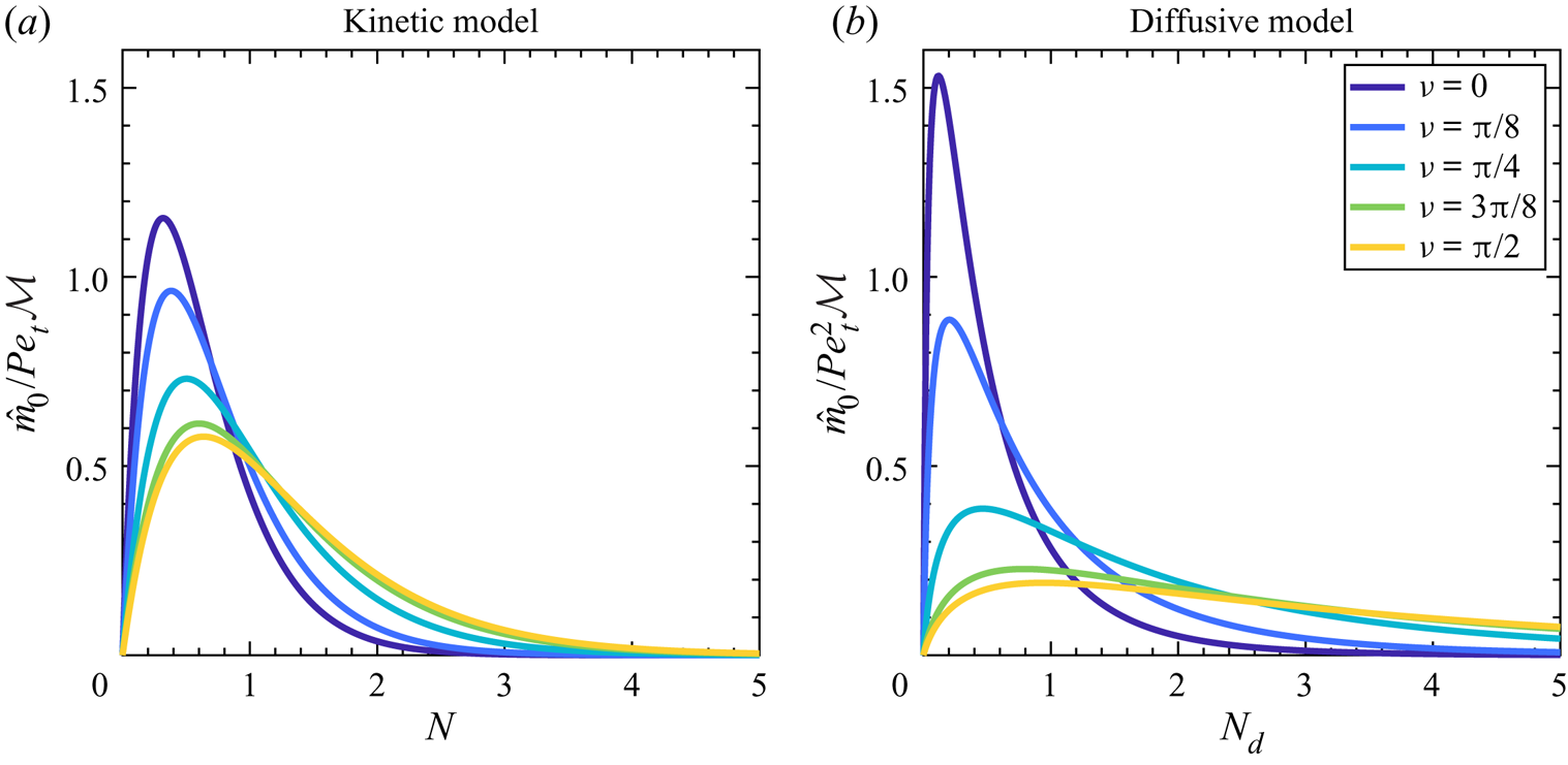
 \begin{equation} \frac{\hat{m}_{0}(s,N,t)}{{{Pe}}_{t}\,\mathcal{M}_{0}(s,0^{+},t)} = \frac{N}{\psi(s)^{2}}\, \text{e}^{{-}N/\psi(s)} = f\left(N;2,\frac{1}{\psi(s)}\right), \quad N = {{Pe}}_{t}\,n, \end{equation}
where  $f(x;k,l) = l^{k}x^{k-1}e^{-lx}/\varGamma (k)$ is the probability density function of a gamma distribution. Note that this is similar to the analysis presented for the axisymmetric droplet in Moore et al. (Reference Moore, Vella and Oliver2021), but with the additional dependence on the droplet geometry through
 $\psi (s)$ and
 $\mathcal {M}_{0}(s,0^{+},t)$.
We can use the similarity form (3.28) to estimate characteristics of the nascent coffee ring to leading order in  $\varepsilon$. In particular, the peak of the solute mass
 $m_{{max}}(s,t)$ (the intensity of the coffee ring) and its location
 $n_{{max}}(s,t)$ are given by
 \begin{equation} m_{{max}}(s,t) = \frac{{{Pe}}_{t}\,\mathcal{M}_{0}(s,0^{+},t)}{\psi(s)\,\text{e}}, \quad n_{{max}}(s,t) = \frac{\psi(s)}{{{Pe}}_{t}}. \end{equation}
A measure of the radial thickness of the nascent coffee ring is given by the full-width at half-maximum,  $w_{1/2}(s)$, which is determined readily from (3.28) to be
 \begin{equation} w_{1/2}(s,t) = n_{{max}}(s,t)\left[W_{0}\left(-\frac{1}{2\text{e}}\right) - W_{{-}1}\left(-\frac{1}{2\text{e}}\right)\right], \end{equation}
where  $W_{0}(x)$ and
 $W_{-1}(x)$ are the Lambert W functions (i.e. solutions of
 $w\,\textrm {e}^{w} = x$, Olver et al. Reference Olver, Lozier, Boisvert and Clark2010). Notably, the ring width is simply a constant fraction of the peak location. Correspondingly, when the peak is located further from the contact line, the ring must be thicker.
In each of (3.28)–(3.30), it is only through  $\psi (s)$ and
 $\mathcal {M}_{0}(s,0^{+},t)$ that any dependence on
 $s$ may arise. To understand asymmetries in the nascent coffee ring, these functions must be understood. One of the aims of the following sections is to investigate them in detail for some specific problems.
3.6. Asymptotic results for a diffusive evaporative flux
Before we move on to validate the asymptotic predictions, we now state the equivalent asymptotic results for the diffusive evaporation model in which the corresponding dimensionless evaporative flux is square-root singular at the contact line, with local expansion given by (2.24). As previously, we may neglect the effects of solute diffusion in the bulk of the droplet, so that the outer solution as described in § 3.1 remains the same as in the kinetic evaporative model. In particular, the local behaviour of the normal velocity (2.25) means that at the contact line,
 \begin{equation} \phi_{0} \sim \frac{B_{d}(s,t)}{\sqrt{n}} \quad \text{as} \ n\rightarrow0^{+}, \end{equation}
where  $B_{d}(s,t)$ is a degree of freedom; we note that this is a weaker singularity than in (3.6).
In addition to weakening the outer solute singularity, (2.25) also necessitates a different scaling for the inner region in which the advective and diffusive fluxes balance, namely
 \begin{equation} n = \varepsilon^{2}\hat{n}_{d}, \quad h = \varepsilon^{2}\hat{h}, \quad \bar{u}_{s} = \varepsilon\hat{u}_{s}, \quad \bar{u}_{n} = \frac{1}{\varepsilon}\,\hat{u}_{n}, \quad \phi = \frac{1}{\varepsilon^{4}}\,\hat{\phi}. \end{equation}
Thus the size of the inner region is an order of magnitude smaller for the diffusive evaporative flux –  $O(\varepsilon ^{2})$ compared to
 $O(\varepsilon )$ – while the solute concentration is two orders of magnitude larger –
 $O(1/\varepsilon ^{4})$ compared to
 $O(1/\varepsilon ^{2})$. This fits with the experimentally observed tendency for a diffusive evaporative flux to produce narrower, higher coffee rings than for a constant evaporative flux (Kajiya et al. Reference Kajiya, Kaneko and Doi2008).
After substituting (3.32a–e) into (2.9)–(2.11) and expanding as  $\varepsilon \rightarrow 0$, the leading-order inner solute concentration is given by
 \begin{equation} \hat{\phi}_{0} = C_{d}(s,t)\exp\left(\frac{-4\chi(s)\,\sqrt{\hat{n}_{d}}}{\theta_{c}(s,t)}\right), \end{equation}
where the coefficient  $C_{d}(s,t)$ can be determined using the integrated mass variable,
 $\mathcal {M}$, in a manner similar to that in which it was determined in the kinetic regime in § 3.2. We find that
 \begin{equation} C_{d}(s,t) = \frac{64\chi(s)^{4}\mathcal{M}_{0}(s,0^{+},t)}{3\theta_{c}(s,t)^{5}}. \end{equation}
To form a composite solution for the solute concentration, we again introduce an intermediate region through the scaling
 \begin{equation} n = \varDelta\mathring{n}_{d}, \quad h = \varDelta\mathring{h}, \quad \bar{u}_{s} = \varDelta^{1/2}\mathring{u}_{s}, \quad \bar{u}_{n} = \frac{1}{\varDelta^{1/2}}\,\mathring{u}_{n}, \quad \phi = \frac{1}{\varepsilon}\,\mathring{\phi}, \end{equation}
where now  $\varepsilon ^{2}\ll \varDelta \ll \varepsilon ^{2/3}$. Again, this range of
 $\varDelta$ is chosen so that we may neglect the lower-order terms in (2.26) in the intermediate region (though again, the solution is independent of the choice of
 $\varDelta$). Pursuing a similar analysis to § 3.3, we find that the corresponding leading-order intermediate solution is given by
 \begin{align} \mathring{\phi}\sim\mathring{\phi}_{0} = \exp\left(-\frac{\varDelta^{1/2}}{\varepsilon}\,\frac{4\chi(s)\sqrt{\mathring{n}_{d}}}{\theta_{c}(s,t)}\right)\left[D_{d}(s,t) + E_{d}(s,t)\,{Ei}\left(\frac{\varDelta^{1/2}}{\varepsilon}\,\frac{4\chi(s)\,\sqrt{\mathring{n}_{d}}}{\theta_{c}(s,t)}\right)\right], \end{align}
as  $\varepsilon,\varDelta \rightarrow 0$ with
 $\mathring {n}=O(1)$, where again
 $D_{d}(s,t)$ and
 $E_{d}(s,t)$ must be determined by matching. The procedure follows in a manner similar to the kinetic case in § 3.3, and we find that
 \begin{equation} D_{d}(s,t) = \frac{64\chi(s)^{4}\mathcal{M}_{0}(s,0^{+},t)}{3\varepsilon^{3}\,\theta_{c}(s,t)^{5}}, \quad E_{d}(s,t) = \frac{4B(s,t)\,\chi(s)}{\theta_{c}(s,t)}. \end{equation}
It follows that an additive composite expansion for the solute concentration profile is given by
 \begin{align} \phi_{{comp}}(x,y,t) & =
\phi_{0}(x,y,t) +
\frac{1}{\varepsilon}\,\frac{4\chi(s)\,B_{d}(s,t)}{\theta_{c}(s,t)}
\exp\left(\frac{-4\chi(s)\,\sqrt{n}}{\varepsilon\,\theta_{c}(s,t)}\right){Ei}\left(\frac{4\chi(s)\,\sqrt{n}}{\varepsilon\,\theta_{c}(s,t)}\right)
\nonumber\\ & \quad +
\frac{1}{\varepsilon^{4}}\,\frac{64\chi(s)^{4}\mathcal{M}_{0}(s,0^{+},t)}{3\theta_{c}(s,t)^{5}}
\exp\left(\frac{-4\chi(s)\,\sqrt{n}}{\varepsilon\,\theta_{c}(s,t)}\right)
- \frac{B_{d}(s,t)}{\sqrt{n}} \nonumber\\ & \quad
-\frac{1}{\varepsilon}\,\frac{4\chi(s)\,B_{d}(s,t)}{\theta_{c}(s,t)}
\exp\left(\frac{-4\chi(s)\,\sqrt{n}}{\varepsilon\,\theta_{c}(s,t)}\right)\log\left(\frac{4\chi(s)\,\sqrt{n}}{\varepsilon\,\theta_{c}(s,t)}\right).
\end{align}
As in the kinetic regime, we note that the final term is included so that the composite solution remains asymptotic throughout the whole drop.
The equivalent similarity profile for the nascent coffee ring in the diffusive evaporative regime is given by
 \begin{equation} \frac{\hat{m}_{0}(s,N_{d},t)}{{{Pe}}_{t}^{2}\,\mathcal{M}_{0}(s,0^{+},t)} = \frac{2\chi(s)}{3\psi(s)}\,f\left(\sqrt{N_{d}},3,\frac{4\chi(s)}{\psi(s)}\right), \quad N_{d} = {{Pe}}_{t}^{2}\,n, \end{equation}
where the shape function of the gamma distribution is now  $3$ compared to
 $2$ in the kinetic regime. The coffee-ring peak
 $m_{{max}}(s,t)$ and its location
 $n_{{max}}(s,t)$ are
 \begin{equation} m_{{max}}(s,t) = \frac{16 {{Pe}}_{t}^{2}\,\mathcal{M}_{0}(s,0^{+},t)\,\chi(s)^{2}}{3\psi(s)^{2}\, \text{e}^{2}}, \quad n_{{max}}(s,t) = \frac{\psi(s)^{2}}{4{{Pe}}_{t}^{2}\,\chi(s)^{2}}, \end{equation}
with the full-width at half-maximum given by
 \begin{equation} w_{1/2}(s,t) = n_{{max}}(s,t)\left[W_{{-}1}\left(\frac{-1}{\sqrt{2}\,\text{e}}\right)^{2} - W_{0}\left(\frac{-1}{\sqrt{2}\,\text{e}}\right)^{2}\right], \end{equation}
so that, again, the ring is thicker the further the peak location is from the contact line.
Note that the similarity form and the properties of the nascent coffee ring for both kinetic and diffusive evaporation depend strongly on the behaviour of the local droplet contact angle through  $\psi (s)$ and the accumulated mass flux into the boundary
 $\mathcal {M}_{0}(s,0^{+},t)$. In the diffusive regime, the heterogeneity of evaporation,
 $\chi (s)$, also plays a role. In § 4, we discuss to what extent each factor is relevant in determining the shape of the coffee ring for a specific example. We will also utilize the asymptotic results to discuss the limitations of the dilute assumption, in particular investigating the role that droplet geometry has on the breakdown of the model.
3.7. Validation for an axisymmetric droplet
We now seek to validate our results by comparing to the axisymmetric case in which  $\varOmega$ is simply circular, given by
 $r = \sqrt {x^{2}+y^{2}} \leq 1$. This case was dealt with in detail by Moore et al. (Reference Moore, Vella and Oliver2021) by proceeding to higher order in the inner region rather than by introducing an intermediate region (as in § 3.3), so that the resulting composite expansions (in §§ 3.4 and 3.6) are different. In this subsection, we validate them by showing excellent agreement with the numerical simulations of Moore et al. (Reference Moore, Vella and Oliver2021).
3.7.1. Kinetic regime
The simplified geometry allows us to evaluate the leading-order flow solution explicitly. In the kinetic evaporative regime, (2.15)–(2.20) give
 \begin{equation} H = \frac{1-r^{2}}{4}, \quad P = P_{0} - \frac{48}{1-r^{2}}, \quad \bar{u}_{r} = \frac{{\rm \pi} r}{4(1-t)}, \quad t_{f} = \frac{1}{\rm \pi}, \quad \alpha = \frac{8}{\rm \pi}. \end{equation}
Here,  $P_{0}$ is an arbitrary constant and
 $\bar {u}_{r}$ is the radial velocity. (We note that there is a slight difference between (3.42a–e) and the corresponding results in Moore et al. (Reference Moore, Vella and Oliver2021); this is due to the fact that the droplet aspect ratio
 $\delta$ in that paper is defined so that it contains an additional
 $2/{\rm \pi}$.)
Now, noting that for an axisymmetric droplet,  $s = \theta$,
 $n = 1-r$,
 $\kappa = -1$ and
 $\bar {u}_{n} = -\bar {u}_{r}$, we can use (3.42a–e) to determine the leading-order solute concentration in each region, finding from (3.1a,b), (3.10) and (3.24),
 $$\begin{gather} \phi_{0} = \frac{1}{\sqrt{1-t}}\left(\frac{1-\sqrt{1-t}\,r^{2}}{1-r^{2}}\right), \end{gather}$$
 $$\begin{gather}\hat{\phi}_{0} = \frac{{\rm \pi}^{2}}{64(1-t)^{3}}\left[1-\sqrt{1-t}-\frac{t}{2}\right]\exp\left(\frac{-{\rm \pi}(1-r)}{4\varepsilon(1-t)}\right), \end{gather}$$
 $$\begin{gather}\mathring{\phi}_{0} = \exp\left(\frac{-{\rm \pi}(1-r)}{4\varepsilon(1-t)}\right)\left[\frac{{\rm \pi}^{2}}{64\varepsilon}\,\frac{(1-\sqrt{1-t}-t/2)}{(1-t)^{3}} +\frac{\rm \pi}{8}\,\frac{(1-\sqrt{1-t})}{(1-t)^{3/2}}\,{Ei}\left(\frac{{\rm \pi}(1-r)}{4\varepsilon(1-t)}\right)\right]. \end{gather}$$
Combining these expressions and evaluating the overlap contributions, we find that an additive composite expansion for the solute concentration is given by
 \begin{align} \phi_{{comp}} & = \phi_{0}(r,t) + \frac{1}{\varepsilon}\,\mathring{\phi}_{0}(r,t) + \frac{1}{\varepsilon^{2}}\hat{\phi}_{0}(r,t) - \frac{(1-\sqrt{1-t})}{2\sqrt{1-t}}\,\frac{1}{1-r} \nonumber\\ & \quad -\frac{1}{\varepsilon^{2}}\,\frac{{\rm \pi}^{2}(1-\sqrt{1-t}-t/2)}{64(1-t)^{3}}\exp\left(-\frac{{\rm \pi}(1-r)}{4\varepsilon(1-t)}\right) \nonumber\\ & \quad -\frac{1}{\varepsilon}\,\frac{\rm \pi}{8}\,\frac{(1-\sqrt{1-t})}{(1-t)^{3/2}}\exp\left(-\frac{{\rm \pi}(1-r)}{4\varepsilon(1-t)}\right)\log\left(\frac{{\rm \pi}(1-r)}{4\varepsilon(1-t)}\right). \end{align}
It is worth noting that the composite solution presented here is valid only to  $O(1/\varepsilon ^{2})$ in the inner region, while the composite solution derived by Moore et al. (Reference Moore, Vella and Oliver2021) is valid to
 $O(1)$.
3.7.2. Diffusive regime
Similarly, in the diffusive regime, (2.15)–(2.20) give
 \begin{align} \left. \begin{aligned}
H & = \frac{1-r^{2}}{4}, \quad \bar{u}_{r} =
\frac{1}{r(1-t)}\left(\frac{1}{\sqrt{1-r^{2}}} -
(1-r^{2})\right), \quad t_{f} = \frac{1}{4}, \quad \alpha =
\frac{8}{\rm \pi}, \\ P & = P_{0} -
\frac{384}{\rm \pi}\left[\frac{1}{\sqrt{1-r^{2}}} +
\frac{1}{3(1-r^{2})^{3/2}} -
\frac{1}{2}\log\left(\frac{1-\sqrt{1-r^{2}}}{1+\sqrt{1-r^{2}}}\right)
+ \log\left(\frac{r}{\sqrt{1-r^{2}}}\right)\right],
\end{aligned} \right\}
\end{align}
where again,  $P_{0}$ is an arbitrary constant. The leading-order solute concentrations in the outer, inner and intermediate regions are then given by
 \begin{align} \phi_{0} & = \frac{1}{(1-t)^{1/4}\sqrt{1-r^{2}}}\left[1-(1-t)^{3/4}(1-(1-r^{2})^{3/2})\right]^{1/3}, \end{align}
 \begin{align} \hat{\phi}_{0} & = \frac{1}{24(1-t)^{5}}\left(1-(1-t)^{3/4}\right)^{4/3}\exp\left(-\frac{\sqrt{2(1-r)}}{\varepsilon(1-t)}\right), \end{align}
 \begin{align} \mathring{\phi}_{0} & = \exp\left(-\frac{\sqrt{2(1-r)}}{\varepsilon(1-t)}\right)\left[\frac{1}{24\varepsilon^{3}(1-t)^{5}}\left(1-(1-t)^{3/4}\right)^{4/3} \right. \nonumber\\ & \quad\left. + \frac{1}{(1-t)^{5/4}}\left(1-(1-t)^{3/4}\right)^{1/3}{Ei}\left(\frac{\sqrt{2(1-r)}}{\varepsilon(1-t)}\right)\right]. \end{align}
We can use these to form an additive composite expansion, given by
 \begin{align} \phi_{{comp}} & = \phi_{0}(r,t) + \frac{1}{\varepsilon}\,\mathring{\phi}_{0}(r,t) + \frac{1}{\varepsilon^{4}}\,\hat{\phi}_{0}(r,t) - \frac{1}{\sqrt{2}(1-t)^{1/4}\sqrt{1-r}}\left(1-(1-t)^{3/4}\right)^{1/3} \nonumber\\ & \quad -\frac{1}{\varepsilon^{4}}\,\frac{1}{24(1-t)^{5}}\left(1-(1-t)^{3/4}\right)^{4/3}\exp\left(-\frac{\sqrt{2(1-r)}}{\varepsilon(1-t)}\right) \nonumber\\ & \quad -\frac{1}{\varepsilon}\,\frac{1}{(1-t)^{5/4}}\left(1-(1-t)^{3/4}\right)^{1/3}\exp\left(-\frac{\sqrt{2(1-r)}}{\varepsilon(1-t)}\right)\log\left(\frac{\sqrt{2(1-r)}}{\varepsilon(1-t)}\right). \end{align}
3.7.3. Comparisons to numerical results
To check the validity of our asymptotic analysis, we compare profiles of the solute mass  $m = h\phi _{{comp}}$ against a numerical solution of (2.9)–(2.11). While the axisymmetry greatly facilitates the numerical solution, the thinness of the boundary layer as discussed in § 3.2 means that care has to be taken with resolution close to the contact line: we use the numerical scheme validated in Moore et al. (Reference Moore, Vella and Oliver2021).
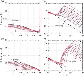
The results are shown for  ${{Pe}} = 200$ in figure 2. In the figure, one can clearly see the transport of the solute mass from the droplet bulk towards the contact line as the droplet evaporates, leading to ring formation in the boundary layer. Moreover, it is evident that the asymptotics do an excellent job of capturing the dynamics, particularly as
 $t$ increases. This gives us confidence in using our asymptotic results to consider the nascent coffee-ring characteristics for more complicated geometries, where numerical solutions of (2.9)–(2.11) are much more computationally challenging (see, for example, Sáenz et al. Reference Sáenz, Wray, Che, Matar, Valluri, Kim and Sefiane2017).
Profiles of the solute mass as an axisymmetric droplet evaporates under (a,b) a kinetic evaporative flux, and (c,d) a diffusive evaporative flux with  ${{Pe}} = 200$. In each panel, the bold black curve represents the initial mass profile
 $m(r) = 2(1-r^{2})/{\rm \pi}$. Also shown are plots at time intervals of 0.1 up to
 $t = 0.9$ in which solid blue curves represent the results from the numerical solution of (2.9)–(2.11), and dashed red curves show the composite mass profiles
 $m = h\phi _{{comp}}$. Panels (b,d) display a doubly-logarithmic plot of the mass profile near the contact line.

4. Droplets with an elliptical contact set
For the rest of this paper, we will specialize to droplets that have an elliptical contact set, namely those given by
 \begin{equation} \varOmega = \left\{(x,y)\left|\left(\frac{x}{1+a}\right)^{2} + y^{2} \leq 1\right.\right\}, \end{equation}
where  $a \geq 0$ is a constant that encodes the eccentricity,
 $e(a) = [a(2+a)]^{1/2}/(1+a)$, of the ellipse.
The forthcoming analysis is more readily approached by introducing the planar elliptical coordinate system  $(\mu,\nu )$, which is defined by
 \begin{equation} x = \sqrt{2a+a^{2}}\cosh\mu\cos\nu, \quad y = \sqrt{2a+a^{2}}\sinh\mu\sin\nu, \end{equation}
where  $0 \leq \mu \leq \mu ^{*} = \textrm {acosh}(1/e(a))$, and
 $\mu = \mu ^{*}$ represents the contact line. We use the symmetry of the problem to restrict our analysis to the quarter of the ellipse in the first quadrant for which the fluid domain transforms to the rectangle
 $0\leq \mu \leq \mu ^{*}$,
 $0\leq \nu \leq {\rm \pi}/2$.
We note that in terms of  $(\mu,\nu )$, the local coordinate system defined in § 2.3 is given by
 \begin{align} \left. \begin{aligned} s(\nu) & = E(\nu,\text{i}\sqrt{2a+a^{2}}), \\ n(\mu,\nu)^{2} & = (2a+a^{2})[(\cosh\mu^{*}-\cosh\mu)^{2}\cos^{2}\nu +(\sinh\mu^{*}-\sinh\mu)^{2}\sin^{2}\nu], \end{aligned} \right\} \end{align}
where  $E(\phi,k) = \int _{0}^{\phi } (1-k^{2}\sin ^{2}\theta )^{1/2}\,\textrm {d}\theta$ is the incomplete elliptic integral of the second kind, with amplitude
 $\phi$ and elliptic modulus
 $k$.
Unlike the case of an axisymmetric drop, the  $(s,n)$-coordinate system is not well-defined throughout the whole quarter-ellipse. For the system to be well-defined at a point, we require a unique normal through that point, and hence a unique value of
 $(s,n)$. This is true everywhere in the quarter-ellipse aside from the interval
 $0 \leq x \leq 1-1/(1+a)$ along the semi-major axis, so that we need
 $1/(1+a) \gg 1/{{Pe}}$ (or
 $1/{{Pe}}^{2}$ for the diffusive regime) for our analysis in § 3.2 to be valid. This is satisfied (for
 ${{Pe}}\gg 1$) provided that
 $a\ll {{Pe}}$, so our analysis is limited to eccentricities
 $e(a) \lesssim 1-1/2{{Pe}}^{2}$. We also note that since the relation between
 $s$ and
 $\nu$ in (4.3) is independent of
 $\mu$, we can use these interchangeably in the rest of our analysis; for convenience, we will use
 $\nu$. It is also important to note that both (4.2a,b) and (4.3) are contact set dependent, in that they change with
 $a$. In particular, while
 $\nu$ indicates heuristically the angular position of a particular point, the
 $\nu$-coordinate of a point with one ellipse eccentricity is not the same for an ellipse with a different eccentricity; the exceptions to this are the points on the semi-major and semi-minor axes, for which
 $\nu = 0$ and
 $\nu = {\rm \pi}/2$ for all
 $a$. Hence in the following, when we wish to make explicit comparisons between different ellipses, we will focus on the semi-axes; happily, this is also where the effects of contact line curvature are seen most clearly.
Our aim in this section is to illustrate the effect of the droplet geometry on the nascent coffee ring. To effect sensible comparisons for elliptical contact sets with different eccentricities, we will consider droplets that have the same initial volume,  $V^{*}$, and contact line perimeter,
 $P^{*}$. When changing the droplet shape, but keeping
 $V^{*}$ and
 $P^{*}$ fixed, we change the characteristic length scaling,
 $R^{*}$, and velocity scaling,
 $U^{*}$, in our model, as well as the values of
 $\delta$ and
 ${{Pe}}$. Here, we discuss how these change when comparing an axisymmetric droplet to an elliptical droplet of the same volume and perimeter.
For an axisymmetric droplet ( $e(0) = 0$), we denote these quantities by a subscript zero. Thus, taking the characteristic length scale to be the radius of the circular contact set, we have
 \begin{equation} R_{0} = \frac{P^{*}}{2{\rm \pi}}, \quad \delta = \frac{V^{*}}{R_{0}^{*3}}, \quad U^{*}_{0} = \frac{\mathcal{E}^{*}}{\rho\delta_{0}}, \quad {{Pe}}_{0} = \frac{R_{0}^{*}U_{0}^{*}}{D^{*}}. \end{equation}
For an elliptical droplet, recall that we took the dimensional length of the semi-minor axis as our reference length scale for the size of the contact set,  $R^{*}$. This length scale changes with the eccentricity of the droplet as encoded through
 $a$. Therefore, using a subscript
 $a$ to denote the different properties, the equivalent values for an ellipse are given by
 \begin{equation} \left. \begin{aligned} R_{a}^{*} & = 2{\rm \pi} \left(\int_{0}^{2{\rm \pi}}\left[(1+a)^{2}\cos^{2}\theta + \sin^{2}\theta\right]{\rm d}\theta\right)^{{-}1}R_{0}^{*},\\ \delta_{a} & = \frac{\delta_{0}R_{0}^{*3}}{R_{a}^{*3}}, \quad U_{a}^{*} = \frac{\delta_{0}U_{0}^{*}}{\delta_{a}}, \quad {{Pe}}_{a} = \frac{R_{a}^{*}U_{a}^{*}}{R_{0}^{*}U_{0}^{*}}\,{{Pe}}_{0}. \end{aligned} \right\} \end{equation}
4.1. Free surface profile
In an elliptical geometry, the Poisson problem (2.19) can be solved explicitly, yielding
 \begin{align} H = \frac{1}{2}\left(1+\frac{1}{(1+a)^{2}}\right)^{{-}1}\left[1-\frac{2a+a^{2}}{(1+a)^{2}}\cosh^{2}\mu\cos^{2}\nu - (2a+a^{2})\sinh^{2}\mu\sin^{2}\nu\right]. \end{align}
We can use this free surface profile to determine the constant  $\alpha$ used to rescale volume (see (2.18)), finding
 \begin{equation} \alpha = \frac{4}{{\rm \pi}(1+a)}\left(1+\frac{1}{(1+a)^{2}}\right). \end{equation}
It is worth noting that if we expand (4.6) as the contact line is approached,  $\mu ^{*}-\mu \rightarrow 0$, then we have
 \begin{equation} H \sim \frac{1}{(1+a)}\left(1+\frac{1}{(1+a)^{2}}\right)^{{-}1}(1 + (2a+a^{2})\sin^{2}\nu)(\mu^{*}-\mu), \end{equation}
so that, recalling (4.3) to determine  $\mu ^{*}-\mu$ as a function of
 $n$, the rescaled contact angle,
 $\psi (\nu ) = \theta _{c}(\nu,t)/(1-t)$, may be found from (2.22), (4.3) and (4.8) to be
 \begin{equation} \psi(\nu) = \frac{4}{{\rm \pi}(1+a)^{2}}[1 + (2a+a^{2})\sin^{2}\nu]^{1/2}. \end{equation}
4.2. Diffusive evaporative flux and dryout times
As described in Kellogg (Reference Kellogg1929), it is possible to solve the concentration problem (2.13) for an elliptical contact set. The resulting evaporative flux is given by
 \begin{align} E(\mu,\nu) = \frac{1}{K[e(a)]}\left[1-\frac{2a+a^{2}}{(1+a)^{2}}\cosh^{2}\mu\cos^{2}\nu - (2a+a^{2})\sinh^{2}\mu\sin^{2}\nu\right]^{{-}1/2}, \end{align}
where  $K(k) = \int _{0}^{{\rm \pi} /2}(1-k^{2}\sin ^{2}\theta )^{-1/2}\,\textrm {d}\theta$ is the complete elliptic integral of the first kind with elliptic modulus
 $k$. Expanding (4.10) close to the contact line, we have
 $E \sim \chi (\nu )\,n^{-1/2}$ with
 \begin{equation} \chi(\nu) = \frac{1}{K[e(a)]}\left(\frac{1+a}{2}\right)^{1/2}(1 + (2a+a^{2})\sin^{2}\nu)^{{-}1/4}. \end{equation}
The dryout time is evaluated from (2.3), yielding
 \begin{equation} t_{f} = \begin{cases}
\displaystyle{\frac{1}{{\rm \pi}(1+a)}}, & \text{in the kinetic
regime}, \\ \displaystyle{\frac{K[e(a)]}{2{\rm \pi}(1+a)}},
& \text{in the diffusive regime}. \end{cases}
\end{equation}
4.3. Fluid velocity
Unfortunately, no such analytical progress is possible for the pressure problem (2.20), which must be solved numerically for each evaporative model. We have found that a convenient way to approach this is to subtract out the most singular terms in  $P$ at the contact line; we describe this process and the details of our numerical methodology in Appendix A.
We can, however, make some comments about the velocity close to the contact line, making use of the fact that in the local coordinate system, the normal velocity is given by
 \begin{equation} \bar{u}_{n} ={-}\bar{u}_{\mu}. \end{equation}
4.3.1. Kinetic evaporation
For the kinetic evaporative model, we combine (2.23a,b) and (4.9) to show that
 \begin{equation} \bar{u}_{\mu} \sim \frac{{\rm \pi}(1+a)^{2}}{4(1-t)}[1+(2a+a^{2})\sin^{2}\nu]^{{-}1/2}, \end{equation}
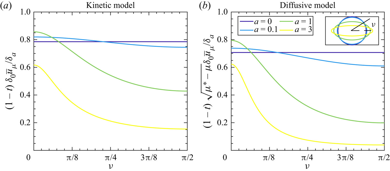
as  $\mu ^{*}-\mu \rightarrow 0$. To illustrate the effects of the droplet geometry on the velocity profile, we display the normal velocity close to the contact line (4.14) as a function of the elliptical polar angle
 $\nu$ in figure 3(a) for different eccentricities. We have scaled
 $(1-t)\bar {u}_{\mu }$ by
 $\delta _{0}/\delta _{a}$ so that for each curve, the droplet has the same initial volume and perimeter, with just the eccentricity of the ellipse changing (cf. (4.5)). The axisymmetric case is illustrated by the purple line. Initially, as we increase
 $a$, it is clear that the velocity is increased in the regions with higher curvature, namely close to the semi-major axis, while being diminished close to the semi-minor axis. However, since
 $\delta _{a}$ increases with
 $a$, eventually the velocity is lower than the equivalent axisymmetric problem around the whole contact line. Nevertheless, the velocity is still relatively stronger along the more highly curved parts of the boundary, and this disparity grows as
 $a$ increases, that is, for more eccentric ellipses, the stronger the flow in the direction of the semi-major axis in comparison to that along the semi-minor axis.
The angular dependence of the normal velocity close to the contact line for (a) a kinetic evaporative model as given by (4.14), and (b) a diffusive evaporative model as given by (4.15). In each panel, we vary the shape of the elliptical contact set by changing  $a$, but scale in such a way that each droplet has the same initial volume and perimeter. For illustration, we show the different droplet footprints in the inset to (b). Displayed are the axisymmetric case,
 $a = 0$ (
 $e(0) = 0$, purple),
 $a = 0.1$ (
 $e(0.1) \approx 0.417$, blue),
 $a = 1$ (
 $e(1) \approx 0.866$, green) and
 $a = 3$ (
 $e(3) \approx 0.968$, yellow).

4.3.2. Diffusive evaporation
Similarly, for a diffusive evaporative model, combining (2.25), (4.3), (4.9) and (4.11) gives
 \begin{equation} \bar{u}_{\mu} \sim \frac{{\rm \pi}(1+a)^{5/2}}{2^{3/2}K(e(a))(1-t)}\,\frac{1}{1+(2a+a^2)\sin^{2}\nu}(\mu^{*}-\mu)^{{-}1/2}, \end{equation}
as  $\mu ^{*}-\mu \rightarrow 0$. We plot
 $(1-t)\sqrt {\mu ^{*}-\mu }\,\delta _{0}\bar {u}_{\mu }/\delta _{a}$ for different ellipse eccentricities in figure 3(b), where we again scale appropriately to fix the initial droplet volume and perimeter. We see very similar behaviour to the kinetic regime: for all ellipse eccentricities, the normal velocity is stronger along the semi-major axis than the semi-minor axis, with this effect being amplified as
 $a$ increases. For
 $a$ small, the velocity is also stronger along the semi-major axis compared to the equivalent axisymmetric droplet, but as
 $a$ gets larger, the velocity is weaker everywhere around the contact line.
4.4. Accumulated mass flux
4.4.1. Kinetic evaporation
We can use the local expansions for the outer solute concentration, (3.6), the contact angle, (4.8), and the velocity, (4.14), together with (4.3)–(4.13) to express the accumulated mass flux into the contact line for a kinetic evaporative model as
 \begin{equation} \mathcal{M}_{0}(\nu,0,t) = \frac{1}{{\rm \pi}(1+a)}[1+(2a+a^{2})\sin^{2}\nu]^{1/2}\int_{0}^{t}B(\nu,\tau)\,{\rm d}\tau. \end{equation}
To investigate how  $\mathcal {M}_{0}$ varies with
 $\nu$ and
 $a$, however, we need to determine
 $B(\nu,t)$, which must be found numerically. The solution procedure is therefore as follows. First, we solve (2.20) numerically to determine
 $\bar {\boldsymbol {u}}$ from (2.17). Since (2.20) is independent of
 $t$, we need do this only once. We can then use the velocity profile to solve the leading-order outer solute problem, (3.1a,b) – again numerically – which then allows us to determine
 $B(\nu,t)$. Finally, we can use
 $B(\nu,t)$ to evaluate the integral in (4.16). The details of the numerical methodologies for each step are recorded in Appendix A.
We display the resulting accumulated mass flux into the contact line (4.16) in figures 4(a,b). In figure 4(a), we display  $\mathcal {M}_{0}$ as a function of the elliptical polar angle
 $\nu$ at different stages of the evaporation for
 $a = 1$. Clearly, even at small times, there is a larger mass flux accumulating along the parts of the contact line with higher curvature, consistent with the results of Freed-Brown (Reference Freed-Brown2015) and Sáenz et al. (Reference Sáenz, Wray, Che, Matar, Valluri, Kim and Sefiane2017). This disparity increases as
 $t$ increases. We display the two extremes by plotting
 $\mathcal {M}_{0}$ along each semi-major axis for various values of the eccentricity
 $a$ in figure 4(b). As previously, we have used the scalings (4.5) to compare droplets that have the same initial volume and contact line perimeter. It is apparent from the figure that as
 $a$ increases, the accumulated mass flux along the semi-major axis increases compared to the axisymmetric case, while the accumulated mass flux along the semi-minor axis decreases compared to the same. These behaviours are accentuated further as the ellipse becomes more eccentric. It is worth stressing that this is in spite of the normal velocity along
 $\partial \varOmega$ being smaller everywhere than in the equivalent axisymmetric problem for large values of
 $a$ (as seen in figure 3a).
The angular dependence of the accumulated mass flux at the contact line under (a,b) a kinetic evaporative flux, as given by (4.16), and (c,d) a diffusive evaporative flux, as given by (4.17). (a,c) Profiles of  $\mathcal {M}_{0}(\nu,0,t)$ at
 $t = 0.1$ (purple),
 $t = 0.2$ (blue),
 $t = 0.4$ (green) and
 $t = 0.8$ (yellow) for an ellipse with
 $a = 1$ (
 $e(1) \approx 0.866$). (b,d) The accumulated mass flux along the semi-major (solid) and semi-minor (dashed) axes for different ellipse eccentricities:
 $a = 0$ (black),
 $a = 0.1$ (
 $e(0.1) \approx 0.417$, purple),
 $a = 1$ (
 $e(1) \approx 0.866$, blue) and
 $a = 3$ (
 $e(3) \approx 0.968$, green). In each of (b,d), we have scaled appropriately so that the droplets have the same perimeter and initial volume.

4.4.2. Diffusive evaporation
The equivalent expression for the accumulated mass flux under a diffusive evaporative model is determined from (4.9), (4.11) and (4.15) to be
 \begin{equation} \mathcal{M}_{0}(\nu,0,t) = \frac{1}{\rm \pi}\sqrt{\frac{1}{2(1+a)}}[1+(2a+a^{2})\sin^{2}\nu]^{{-}1/4}\int_{0}^{t}B_{d}(\nu,\tau)\,{\rm d}\tau. \end{equation}
Again, we must determine  $B_{d}(\nu,\tau )$ numerically by solving the leading-order outer solute advection problem for
 $\phi _{0}$. The procedure is identical to the that in the kinetic regime, and we display the resulting profiles of
 $\mathcal {M}_{0}(\nu,0,t)$ in figures 4(c,d). The broad behaviour of accentuated mass accumulation along the semi-major axis is very similar to the kinetic regime, although it is notable that
 $\mathcal {M}_{0}(\nu,0,t)$ is larger at earlier times in the diffusive regime. While under both evaporative models all of the mass will be driven to the contact line at the dryout time (since diffusion is a lower-order effect in the outer region), the stronger evaporative flux in the diffusive regime means that mass accumulates faster at the contact line in this regime.
4.5. Mass profiles
With the accumulated mass flux  $\mathcal {M}_{0}$ in hand, we are able to construct the leading-order solute mass profiles,
 $m = h\phi _{{comp}}$, using (3.25) in the kinetic regime and (3.38) in the diffusive regime. Our aim is to consider the relative influence of the droplet geometry and the evaporative flux on the resulting coffee-ring profile.
4.5.1. Kinetic evaporation
To isolate the role of geometry-induced fluid flow, we first consider the kinetic evaporative model. We display in figure 5 mass profiles along the semi-minor and semi-major axes for an ellipse with  $a = 1$ (
 $e(1) = 0.866$). The droplet has been chosen to have the same initial volume and perimeter as the axisymmetric droplet depicted in figure 2, so that the equivalent Péclet number is
 ${{Pe}}_{a} \approx 35$. In the figure, the bold black lines represent the initial mass profile, while the blue lines represent the mass profile evolution along the semi-major axis (figure 5a,b) and semi-minor axis (figure 5c,d). As the droplet evaporates, we can see clearly the formation of the nascent coffee ring along both axes, with a characteristic thin, sharp peak growing close to the pinned contact line. It is noticeable that the peak along the semi-major axis is larger than that along the semi-minor axis. At
 $90\,\%$ of the drying time, the coffee-ring peak is approximately three times higher along the semi-major axis than the semi-minor axis. The coffee-ring effect is also enhanced when compared to the axisymmetric case: the peak along the semi-major axis is approximately
 $1.4$ times larger than that for the equivalent axisymmetric droplet shown in figure 2, with the peak on the semi-minor axis approximately
 $2.2$ times smaller.
Profiles of the solute mass  $m = h\phi _{{comp}}$ along the semi-major (a,b) and semi-minor (c,d) axes of an elliptical droplet with
 $a = 1$ (
 $e(1) = 0.866$) evaporating under a kinetic flux for
 ${{Pe}} \approx 35$ (so that the droplet has the same initial volume and perimeter as the axisymmetric droplet shown in figure 2). In each panel, the bold black curve represents the initial mass profile, while plots at time intervals of 0.1 up to
 $t = 0.9$ are shown as solid blue curves. Panels (b,d) display a doubly-logarithmic plot of the mass profiles near the contact line, where we see the formation of the nascent coffee ring as
 $t$ increases. It is notable that the coffee-ring effect is much stronger along the semi-major axis due to the strong accumulated mass flux in this region.

It is also worth noting that the peak along the semi-minor axis is slightly further from the contact line compared to the semi-major axis. For example (and accounting for the rescalings in (4.5)), at  $90\,\%$ of the drying time, the peak along the semi-major axis is at
 $2-x \approx 5.8\times 10^{-4}$, while along the semi-minor axis it is at
 $1-y \approx 1.3\times 10^{-3}$. For reference, the axisymmetric peak location is comparable to the peak on the semi-major axis, with
 $1-r \approx 6.5\times 10^{-4}$ in figure 2.
We further illustrate the effect of ellipse geometry in figures 6(a,b), where we show the variation of the maximum coffee-ring peak (figure 6a) and its distance from the contact line (figure 6b) along each semi-axis with ellipse eccentricity. Each ellipse has the same initial volume and perimeter, with the Péclet number of the axisymmetric drop taken to be  ${{Pe}}_{0} = 200$. The equivalent Péclet numbers for the elliptical drops are then calculated from (4.5). The results are shown at
 $90\,\%$ of the drying time.
Variation with eccentricity of the dimensionless peak coffee-ring height (a,c), and its dimensionless distance from the contact line (b,d), at  $90\,\%$ of the drying time. Each ellipse has the same initial perimeter and volume. We display results for both the kinetic (a,b) and diffusive (c,d) regimes. In each panel, the red squares indicate results for the semi-minor axis, while the blue circles indicate results for the semi-major axis. In the insets to (a,c), we display the ratio of the current peak height at
 $e(a)$ to the equivalent axisymmetric droplet to highlight how increasing the eccentricity of the droplet leads to a local maximum in the peak height.

Initially, as the ellipse eccentricity is increased, the peak height along the semi-major axis increases, until reaching a maximum at  $a \approx 1.5$ (
 $e(a) \approx 0.917$), where it is approximately
 $1.46$ times larger than the equivalent axisymmetric droplet (cf. the inset to figure 6a). For larger eccentricities, the peak height then decreases again, although remaining higher than the axisymmetric case for the eccentricities displayed. It is worth noting that as
 $e(a)$ approaches unity, the assumptions made in deriving the model begin to break down, with the aspect ratio of the droplet contact set becoming larger than
 $O(1)$. Moreover, the Péclet number as given by (4.5) decreases with
 $a$, so the existence of a maximum is not unexpected.
On the other hand, the peak height along the semi-minor axis decreases monotonically as the eccentricity of the ellipse increases. Indeed, as  $e(a)$ gets closer to unity, the rate of decrease of the height gets faster. For
 $a = 3$ (
 $e(a) \approx 0.968$), the peak height along the semi-minor axis has decreased by almost a factor of
 $7$.
Along the semi-minor axis, the location of the coffee-ring peak moves radially inwards away from the pinned contact line of the droplet. Correspondingly, according to the analysis of § 3.5, as the ellipse eccentricity increases, the thickness of the nascent coffee ring as measured by the full-width at half-maximum increases. Along the semi-major axis, the distance of the peak from the contact line location decreases slightly at very small eccentricities, before again becoming larger than the equivalent axisymmetric case as  $e(a)$ approaches unity. The effect is noticeably weaker than that along the semi-minor axis.
Thus, in summary, on the semi-minor axis, as the eccentricity of the ellipse increases, the coffee ring gets progressively shallower and wider compared to an axisymmetric droplet of the same initial volume and perimeter. On the semi-major axis, the coffee ring initially becomes narrower and higher, before transitioning to a ring that is wider and higher than the equivalent axisymmetric droplet.
These behaviours can be probed further by considering the similarity analysis of § 3.5. The local similarity profile is given by (3.28), which becomes
 \begin{align} \frac{\hat{m}_{0}}{{{Pe}}_{t}\,\mathcal{M}_{0}(\nu,0,t)} = \frac{{\rm \pi}^{2}(1+a)^{4}}{16}\,\frac{N}{[1+(2a+a^{2})\sin^{2}\nu]}\exp\left(\frac{-{\rm \pi}(1+a)^{2}N}{4[1+(2a+a^{2})\sin^{2}\nu]^{1/2}}\right), \end{align}
where  $N = {{Pe}}_{t}\,n$, and
 $n$ is given by (4.3). The leading-order coffee-ring peak and its location are found from (3.29) to be
 \begin{align} \frac{m_{{max}}}{{{Pe}}_{t}\,\mathcal{M}_{0}(\nu,0,t)} = \frac{{\rm \pi}(1+a)^{2}}{4\text{e}\,[1+(2a+a^{2})\sin^{2}\nu]^{1/2}}, \quad {{Pe}}_{t}\,n_{{max}} = \frac{4[1+(2a+a^{2})\sin^{2}\nu]^{1/2}}{{\rm \pi}(1+a)^{2}}. \end{align}
It is clear that the right-hand side of (4.19a) is monotonically decreasing in  $\nu$. In particular, its value along
 $\nu = 0$ is
 $(1+a)^{2}$ times larger than that along
 $\nu = {\rm \pi}/2$. Thus the geometry-induced flow alone drives an enhanced coffee ring along the semi-major axis. Moreover, we note that since, for a fixed
 $a$,
 $\mathcal {M}_{0}(\nu,0,t)$ is a decreasing function of
 $\nu$ (cf. figure 3c), including the accumulated mass flux accentuates this effect further.
The peak location and hence the full-width at half-maximum (cf. (3.30)) are independent of the accumulated mass flux, so that their behaviour as functions of  $\nu$ is governed purely by the local free surface profile. As is seen clearly from (4.19b), as
 $\nu$ increases, the ring peak is further from the contact line, leading to a thicker coffee ring. The scale factor in terms of distance from the contact line – and hence thickness of the ring – between the semi-major and semi-minor axes is given by
 $1/(1+a)^{2}$.
All of these features can be seen by plotting the similarity profile (4.18) for a droplet with  $a = 1$ for different values of
 $\nu$, which is shown in figure 7(a): as
 $\nu$ increases, the mass profiles get progressively shallow and broader, with the location of the peak moving away progressively from the contact line at
 $n = 0$. The accumulated mass flux
 $\mathcal {M}_{0}(\nu,0,t)$ simply acts to accentuate the coffee-ring height, with the peak location and the full-width at half-maximum remaining unchanged.


A previous study by Freed-Brown (Reference Freed-Brown2015) demonstrated numerically that the mass flux of solute is stronger along the semi-major axis of a uniformly evaporating elliptical droplet. Here we have expanded upon this study, illustrating clearly that this increased mass flux combines with the effect of the local droplet profile, leading to an enhanced coffee ring along the more highly curved parts of the contact line. Moreover, this is for a constant evaporative flux, showing that this asymmetry in the solute distribution can be driven by geometry-induced flow alone, which may have useful applications in evaporative-driven patterning processes (Harris et al. Reference Harris, Hu, Conrad and Lewis2007).
4.5.2. Diffusive evaporation
If one also allows the evaporative flux to vary as a result of the droplet geometry, then the asymmetries in the nascent coffee ring become more exaggerated. To show this, we plot in figure 8 mass profiles along the semi-minor and semi-major axes for an ellipse with  $a = 1$ (
 $e(1) = 0.866$) evaporating under a diffusive flux (the droplet again has the same initial volume and perimeter as that in figures 2 and 5). The coffee-ring effect is enhanced significantly by the contact line geometry: the peak of the ring at
 $90\,\%$ of the drying time is
 $\approx 13$ times larger along the semi-major axis than the semi-minor axis. Moreover, the peak is also approximately
 $1.1$ times larger than that in the equivalent axisymmetric diffusive problem.
Profiles of the solute mass  $m = h\phi _{{comp}}$ along the semi-major (a,b) and semi-minor (c,d) axes of an elliptical droplet with
 $a = 1$ (
 $e(1) = 0.866$) evaporating under a diffusive flux for
 ${{Pe}} \approx 35$. In each panel, the bold black curve represents the initial mass profile, while plots at time intervals of 0.1 up to
 $t = 0.9$ are shown as solid blue curves.

We illustrate how the properties of the nascent coffee ring vary with ellipse eccentricity in figures 6(c,d), where we show how the ring peak and its distance from the contact line change with  $e(a)$ for a fixed initial droplet volume and perimeter. The results are displayed at
 $90\,\%$ of the drying time, with the Péclet number of the equivalent axisymmetric drop taken to be
 ${{Pe}}_{0} = 200$, and the corresponding parameters for the droplets with elliptical footprints evaluated from (4.5).
The results behave in a qualitatively similar manner to the kinetic regime. In particular, the peak height along the semi-major axis initially increases as we increase the eccentricity, before reaching a maximum. For the diffusive case, the maximum is at  $a \approx 0.5$ (
 $e(a) \approx 0.745)$, with the peak approximately
 $20\,\%$ larger than the equivalent axisymmetric droplet (cf. the inset to figure 6c). As the eccentricity increases further, the peak height begins to decrease again, eventually decreasing below the axisymmetric peak. It is worth noting, however, that the width of the coffee ring is larger than in the equivalent axisymmetric droplet. Hence for larger eccentricities, we have a shallower but wider coffee ring, as necessitated by the overall increased accumulated mass flux into the contact line along the semi-major axis (cf. figure 4).
For a diffusively evaporating droplet, the similarity profile can be found from (3.39) to be given by
 $$\begin{gather} \frac{\hat{m}_{0}}{{{Pe}}_{t}^{2}\,\mathcal{M}_{0}(\nu,0,t)} = \frac{{\rm \pi}^{4}(1+a)^{10}}{48K[e(a)]^{4}}\,\frac{N_{d}}{(1+(2a+a^{2})\sin^{2}\nu)^{3}} \nonumber\\ \times \exp\left(\frac{-{\rm \pi}(1+a)^{5/2}\sqrt{N_{d}}}{K(e(a))\,[1+(2a+a^{2})\sin^{2}\nu]^{3/4}}\right), \end{gather}$$
where  $N_{d} = {{Pe}}_{t}^{2}\,n$. The coffee-ring peak and its location are given by
 $$\begin{gather} \frac{m_{{max}}}{{{Pe}}_{t}^{2}\,\mathcal{M}_{0}(\nu,0,t)} = \frac{{\rm \pi}^{2}(1+a)^{5}}{6 \text{e}^{2}\,K[e(a)]^{2}}\,\frac{1}{[1+(2a+a^{2})\sin^{2}\nu]^{3/2}}, \end{gather}$$
 $$\begin{gather}{{Pe}}_{t}^{2}\,n_{{max}} = \frac{8K[e(a)]^{2}}{{\rm \pi}^{2}(1+a)^{5}}[1+(2a+a^{2})\sin^{2}\nu]^{3/2}. \end{gather}$$
In the diffusive regime, even when we discount the accumulated mass flux into the contact line, there is a more significant strengthening of the coffee-ring effect compared to the kinetic evaporative model. Along the semi-major axis of the ellipse, the peak height is  $(1+a)^{3}$ larger,
 $1/(1+a)^{3}$ closer to the contact line, and
 $1/(1+a)^{3}$ thinner than along the semi-minor axis. This can be seen clearly in figure 7(b), where we plot the similarity profile (4.20) for different values of
 $\nu$. Generally speaking, even though there are variations with the angle-like variable
 $\nu$, the coffee ring in the kinetic regime is much more uniform than that in the diffusive regime.
4.6. Summary
Our findings corroborate those of Sáenz et al. (Reference Sáenz, Wray, Che, Matar, Valluri, Kim and Sefiane2017), who consider experiments and simulations of different-shaped droplets evaporating under the diffusive evaporative model, demonstrating that there is a more pronounced coffee ring near the most highly curved parts of the droplet contact line. While Sáenz et al. (Reference Sáenz, Wray, Che, Matar, Valluri, Kim and Sefiane2017) attribute this to the asymmetry in the evaporative flux (specifically, that it is stronger along these parts of the boundary), we have demonstrated that this is not the only factor; indeed, the similarity profile (4.20) shows that there is an enhanced coffee-ring effect along the semi-major axis of an ellipse due purely to the flow asymmetry induced by the droplet geometry. Thus in the diffusive regime, it is a combined effect of the droplet geometry, the increased mass flux and the increased evaporative flux that contributes to the change in the coffee-ring structure with contact line curvature.
4.7. Limitations of the dilute regime
All of the above results hold under the assumption that the solute remains dilute as it evaporates. However, as solute is carried to the contact line, the concentration increases there. As a result, several effects that we have neglected, most notably concentration-dependent diffusivity and suspension viscosity, become relevant locally. Eventually, the solute may jam, leading to an effective moving of the fluid boundary inwards from the initial pinned edge. While we do not seek to investigate these effects in the current analysis, it is clearly important to understand the limitations of the dilute assumption. Moreover, even if the window over which the dilute model is valid is quite short, it is necessarily the first stage of the coffee-ring formation, so the analysis presented here represents the early-time solution that will apply before these effects become relevant.
4.7.1. Kinetic evaporation
Let us suppose that the critical solute concentration at which finite concentration effects are important is given by  $\phi _{c}^{*}$. This value will depend upon the solute under consideration. For the purposes of illustration, we will assume that
 $\phi _{c}^{*} = 0.1$, while we will take indicative values of the initial concentration from Deegan et al. (Reference Deegan, Bakajin, Dupont, Huber, Nagel and Witten2000), with
 $\phi _{{init}}^{*}$ ranging from
 $10^{-6}$ to
 $10^{-2}$.
Now, according to our asymptotic analysis, the maximum value of the solute concentration,  $\phi _{{max}}(t)$, occurs at the contact line. Thus we can evaluate the composite profile (3.25) on
 $\partial \varOmega$ to find that
 \begin{equation} \phi_{{max}}(\nu,t) = {{Pe}}^{2}\,\frac{\mathcal{M}_{0}(\nu,0,t)}{\theta_{c}(\nu,t)^{3}} + {{Pe}}\,\frac{\gamma\,B(\nu,t)}{\theta_{c}(\nu,t)}+ \lim_{\substack{(x,y)\rightarrow\partial\varOmega \\ n\rightarrow 0}} \left(\phi_{0}(x,y,t) - \frac{B(\nu,t)}{n}\right), \end{equation}
where  $\gamma$ is the Euler–Mascheroni constant.
Note that  $\phi _{{max}}$ depends on the elliptical polar angle; our previous analysis has indicated that the maximum is higher along the semi-major axis of the ellipse than along the semi-minor axis, and we expect this to translate directly into a reduced range of validity of the dilute model. To investigate this, in figure 9 we plot
 $\phi _{{max}}(\nu,t)$ as a function of time for an elliptical droplet with
 $a = 1$ and for different Péclet numbers. In each panel, the value of
 $\phi _{{max}}(\nu,t)$ along the semi-major axis is given by the dashed curve, while its value along the semi-minor axis is given by the dotted curve. For reference, the equivalent maximum concentration for an axisymmetric droplet of the same volume and perimeter is shown in each panel by the solid curve. Figures 9(a–c) show the results for
 ${{Pe}} = 200, 400, 800$, respectively, which are defined with respect to the axisymmetric droplet, and the corresponding Péclet number for the elliptical case can be found using (4.5). To help interpret the results, we have also included reference values of
 $\phi _{c} = \phi _{c}^{*}/\phi _{{init}}^{*}$ as the dashed red lines.
The maximum solute concentration,  $\phi _{{max}}(\nu,t)$, for an elliptical droplet with
 $a = 1$ (
 $e(a) = 0.866$) evaporating under a constant evaporative flux as given by (4.23). In each plot, the dashed curve displays the maximum concentration on the semi-major axis,
 $\phi _{{max}}(0,t)$, the dotted curve displays the concentration on the semi-minor axis,
 $\phi _{{max}}({\rm \pi} /2,t)$, and the solid curve shows the equivalent results for an axisymmetric droplet of the same volume and perimeter. The results are shown for (a)
 ${{Pe}} = 200$, (b)
 ${{Pe}} = 400$, (c)
 ${{Pe}} = 800$, where the Péclet number is defined with respect to the axisymmetric droplet. In each panel, the horizontal dashed red lines denote particular values of the critical concentration
 $\phi _{c}$. For each curve, the dilute regime lies to the left of the intersection with the red lines.

As is seen clearly in figure 9, our intuition is correct: for a given value of  $\phi _{c}$, the solute concentration along the semi-major axis reaches the critical value much earlier than along the semi-minor axis. Moreover, compared to an axisymmetric droplet of the same volume and contact line length, the critical solute concentration is reached sooner along the semi-major axis and later on the semi-minor axis. For a fixed
 ${{Pe}}$, the time window over which the dilute regime remains valid increases as
 $\phi _{c}$ increases, while for a fixed
 $\phi _{c}$, the time window decreases as
 ${{Pe}}$ increases.
To take a concrete example, let us consider  $\phi _{c} = 10^{5}$, which corresponds to a solute that is initially extremely dilute compared to the critical concentration. For
 ${{Pe}} = 200$, the dilute regime is valid for
 $\approx 80\,\%$ of the drying time for an axisymmetric drop, while for an elliptical drop, the dilute regime breaks down after
 $\approx 76\,\%$ of the drying time along the semi-major axis, and after
 $\approx 87\,\%$ of the drying time along the semi-minor axis. On the other hand, for
 ${{Pe}} = 800$, the dilute regime is valid for
 $\approx 60\,\%$ of the drying time for an axisymmetric drop, while it breaks down after
 $\approx 55\,\%$ of the drying time along the semi-major axis, and after
 $\approx 75\,\%$ of the drying time along the semi-minor axis, for the equivalent elliptical drop.
It is of note that in each of these cases, the dilute regime takes up a large percentage of the total drying time, indicating that the asymptotic analysis that we have presented here gives a very good account of the nascent coffee-ring formation and, in particular, allows us to predict the solute mass distribution within the droplet when finite concentration effects start to become relevant. Moreover, the solute mass profiles presented in, for example, § 4.5, would be apt for comparison to experimental measurements of transient coffee-ring profiles for an elliptical droplet evaporating under a kinetic evaporative flux.
However, it is worth noting that the time windows over which the dilute regime is valid do significantly reduce as  $\phi _{c}$ decreases. For
 ${{Pe}} = 200$ and
 $\phi _{c} = 10$, breakdown occurs after
 $\approx 8\,\%$ of the drying time for the axisymmetric droplet,
 $\approx 5\,\%$ of the drying time along the semi-major axis of the equivalent elliptical droplet, and
 $\approx 18\,\%$ of the drying time along the semi-minor axis. Nevertheless, our analysis is appropriate for the time window before breakdown, and provides the initial conditions for the regime in which finite concentration effects are relevant, so it is likely to be an important consideration in understanding the characteristics of the final coffee ring.
We should also note that it may be that finite concentration effects are extremely localized in the model, so that, for example, even in problems where they are relevant close to the highly curved parts of the contact line, the dilute model may still give an excellent description of the coffee-ring dynamics for other parts of the boundary. This seems particularly reasonable given that the solute simply follows the streamlines in the droplet bulk (where the dilute regime is still valid), and the streamlines are independent of  $t$. However, these comments do depend on the type of model chosen to incorporate finite concentration effects, and whether such a model causes non-local changes to the liquid flow. We do not seek to address these questions any further here.
4.7.2. Diffusive evaporation
By the composite solution (3.38), the maximum concentration in the diffusive evaporative regime is given by
 $$\begin{gather} \phi_{{max}}(\nu,t) =
{{Pe}}^{4}\,\frac{64\chi(\nu)^{4}\,\mathcal{M}_{0}(\nu,0,t)}{3\theta_{c}(\nu,t)^{5}}+
{{Pe}}\,\frac{4\gamma\,\chi(\nu)\,B_{d}(\nu,t)}{\theta_{c}(\nu,t)}\nonumber\\
+ \lim_{\substack{(x,y)\rightarrow\partial\varOmega\\
n\rightarrow 0}} \left(\phi_{0}(x,y,t) - \frac{B_{d}(\nu,t)}{\sqrt{n}}\right). \end{gather}$$
It is apparent immediately that this is two orders of magnitude larger than (4.23) and, accordingly, the time window over which the dilute regime is valid for this mode of evaporation is much smaller, as can be seen in figure 10. For  ${{Pe}} = 200$ and
 $\phi _{c} = 10^{5}$, we see that breakdown occurs for an axisymmetric droplet at just
 $\approx 1\,\%$ of the drying time, with this value decreasing rapidly as
 $\phi _{c}$ decreases or
 ${{Pe}}$ increases. Breakdown along the semi-major axis of the equivalent ellipse occurs at a similar time, while there is an appreciable increase in the validity of the dilute model along the semi-minor axis to
 $\approx 23\,\%$ of the drying time. Again, this tails off sharply as
 $\phi _{c}$ decreases. Hence if finite concentration effects can be treated locally, then we may see a sizeable time frame over which the dilute model presented here gives an accurate description of the nascent coffee ring along parts of the contact line with smaller curvature. Overall, however, it is clear that we need to consider these effects much sooner in the diffusive evaporative flux regime.
The maximum solute concentration,  $\phi _{{max}}(\nu,t)$, for an elliptical droplet with
 $a = 1$ (
 $e(a) = 0.866$) evaporating under a diffusive flux as given by (4.24). In each plot, the dashed curve displays the maximum concentration on the semi-major axis,
 $\phi _{{max}}(0,t)$, the dotted curve displays the concentration on the semi-minor axis,
 $\phi _{{max}}({\rm \pi} /2,t)$, and the solid curve shows the equivalent results for an axisymmetric droplet of the same volume and perimeter. The results are shown for (a)
 ${{Pe}} = 200$, (b)
 ${{Pe}} = 400$, (c)
 ${{Pe}} = 800$, where the Péclet number is defined with respect to the axisymmetric droplet. In each panel, the horizontal dashed red lines denote particular values of the critical concentration
 $\phi _{c}$.

It is noticeable that there is marginal difference between the breakdown time along the semi-major axis and the equivalent axisymmetric droplet, and indeed some cases where it appears to be reduced along the semi-major axis compared to the axisymmetric case. Given the extremely small time frames under consideration, this is likely a combined effect of the numerical sensitivities in evaluating  $\mathcal {M}_{0}(\nu,0,t)$ and
 $B_{d}(\nu,t)$, and the fact that the equivalent Péclet numbers are significantly smaller for an elliptical droplet (cf. (4.5)).
5. Summary and discussion
In this paper, we have presented a systematic asymptotic analysis of the solute profile as a thin surface-tension-dominated droplet of arbitrary contact set evaporates in the limit of large solutal Péclet number,  ${{Pe}}\gg 1$. Throughout, we have assumed that the droplet contact line remains pinned as the droplet evaporates. To illustrate the mathematical methodology, we focused on two particular evaporation models that are expected to bracket the most common evaporative behaviours: a simplified kinetic evaporation model in which the flux is uniform above the droplet surface, and a diffusive evaporation model in which the flux is singular at the contact line. In the former case, we were able to isolate the effect of the droplet geometry alone on the nascent coffee-ring characteristics, while for the latter regime, we were able to investigate the combined effects of the droplet geometry and an inhomogeneous evaporative flux.
Our analysis builds upon our previous work (Moore et al. Reference Moore, Vella and Oliver2021), which revealed that it is the competing effects of solute diffusion and advection local to the contact line that drive the formation of the characteristic coffee-ring profile in the early stages of evaporation. In a more general geometry, the analysis is significantly more challenging, but we were able to make asymptotic progress by utilizing a local orthogonal coordinate system  $(s,n)$ that is embedded in the droplet contact line. This allows us to solve the leading-order local solute transport problem explicitly. To match with the advection-dominated region of the droplet, we exploited a formulation in terms of an integrated mass variable, which revealed that the local coffee-ring profile is approximately a similarity profile
 $\hat {m}_{0}$ that is given by
 \begin{equation} \frac{\hat{m}_{0}(s,N,t)}{{{Pe}}_{t}\,\mathcal{M}_{0}(s,0^{+},t)} = f\left(N;2,\frac{1}{\psi(s)}\right), \quad N = {{Pe}}_{t}\,n \end{equation}
for a kinetic evaporative flux, and by
 \begin{equation} \frac{\hat{m}_{0}(s,N_{d},t)}{{{Pe}}_{t}^{2}\,\mathcal{M}_{0}(s,0^{+},t)} = \frac{2\chi(s)}{3\psi(s)}\,f\left(\sqrt{N_{d}},3,\frac{4\chi(s)}{\psi(s)}\right), \quad N_{d} = {{Pe}}_{t}^{2}\,n \end{equation}
for a diffusive evaporative flux. In (5.1) and (5.2),  $\mathcal {M}_{0}(s,0^{+},t)$ is the mass accumulated at the contact line,
 $\psi (s) = \theta _{c}(s,t)/(1-t)$ is the rescaled local contact angle of the droplet,
 $\chi (s) \sim E(s,n)\,n^{1/2}$ is the strength of the singularity in the local evaporative flux in the diffusive regime,
 $f(x;k,l) = l^{k}x^{k-1}\,\textrm {e}^{-lx}/\varGamma (k)$ is the probability density function of a gamma distribution,
 ${{Pe}}_{t} = {{Pe}}/(1-t^{*}/t_{f}^{*})$ is the modified Péclet number, and
 $t_{f}^{*}$ is the dimensional dryout time of the drop. Characteristics of the nascent coffee ring such as the ring height and width can then be found readily from these similarity profiles.
Equations (5.1) and (5.2) display the characteristic narrow peaked profile of the nascent coffee ring, and it is notable that this profile is dependent on the location on the contact line through the coordinate  $s$. Hence asymmetry in the droplet profile, the evaporative flux and the rate at which solute mass is transported to the contact line may all contribute to variation in the nascent coffee-ring profile.
After validating our asymptotic analysis in the axisymmetric regime by comparing to numerical simulations, we moved on to consider the example of a thin droplet with an elliptical contact set. For both evaporative models, the flow in the ellipse is stronger towards the semi-major axis where the contact line curvature is higher, and this effect is accentuated as the eccentricity of the ellipse increases. The increased velocity coupled with the geometry of the local free surface profile leads to an increase in the accumulated mass flux into the more highly curved part of the elliptical boundary. We showed that for droplets of identical volume and contact line perimeter, increasing the ellipse eccentricity increases (respectively, decreases) the accumulated mass flux into the boundary along the semi-major (semi-minor) axis. This effect was more pronounced (although of a similar order of magnitude) for a diffusive evaporative flux. The increased accumulated mass flux contributes to a strengthened (respectively, weakened) coffee ring along the semi-major (semi-minor) axis.
It is notable that this effect is exhibited by both the kinetic and diffusive evaporative models. In particular, while it certainly contributes if present, inhomogeneity in the evaporative flux is not necessary to observe a variation in the coffee-ring effect. This qualifies the conclusion of Sáenz et al. (Reference Sáenz, Wray, Che, Matar, Valluri, Kim and Sefiane2017) that attributes coffee-ring asymmetry to an inhomogeneous evaporative flux.
For both evaporative models, the decreased mass flux into the contact line along the semi-minor axis manifests itself as a shallower, wider coffee ring than an equivalent axisymmetric droplet of the same initial volume and perimeter. However, the behaviour along the semi-major axis is richer. As the eccentricity of the droplet contact set increases initially, for both evaporative models the coffee ring becomes higher and narrower. The height reaches a maximum before falling in both evaporation models, with the effect starker for diffusive evaporation. However, to compensate for the increased mass flux, the ring then starts to broaden as compared to the axisymmetric droplet. As the eccentricity of the ellipse approaches unity, in the kinetic model, we found that the coffee-ring height was comparable to the axisymmetric droplet, but the ring was thicker, while for the diffusive model, we found that the height was in fact lower than the axisymmetric droplet, but the ring was much thicker.
We concluded by using our asymptotic results to investigate when the dilute regime breaks down and finite concentration effects are likely to become relevant close to the contact line, where the solute concentration is maximal. As may be expected, the enhanced flow and coffee-ring effect along the semi-major axis reduces the time window over which the dilute model is valid as compared to the equivalent axisymmetric droplet. However, this effect is very much localized; indeed, along the semi-minor axis, the time window is lengthened correspondingly. Clearly, finite concentration effects may be present in some parts of the droplet for a significantly longer period than others. It is notable that the dilute regime is valid for significantly longer for a kinetic evaporative flux compared to a diffusive flux; this is due to the significantly enhanced coffee-ring effect in the latter regime. This longer time period of validity coupled with the variable coffee-ring effect along different parts of the contact line suggests that the kinetic evaporative model may be ripe for exploitation in engineering applications in which controlling the deposit shape dynamically is important, for example in colloidal patterning (Choi et al. Reference Choi, Stassi, Pisano and Zohdi2010) and in printing conductors (Layani et al. Reference Layani, Gruchko, Milo, Balberg, Azulay and Magdassi2009).
Even in situations where the time window of applicability is relatively small, the dilute model necessarily applies in the early stages of coffee-ring formation. Hence the analysis derived here provides a description of the flow profile and solute distribution before finite concentration effects are introduced. There are a number of different avenues that could be pursued to model such effects, whether through a simple jamming model (such as that in Popov Reference Popov2005), accounting for the increasing concentration through suspension-dependent viscosity and diffusivity (as in Kaplan & Mahadevan Reference Kaplan and Mahadevan2015), or through more complicated two-phase suspension models (see, for example, Guazzelli & Pouliquen Reference Guazzelli and Pouliquen2018). These are all interesting avenues for future studies.
There are also a number of other possible extensions of the model presented here to account for some of the physical effects that have been neglected. First, we have shown that the evaporative flux law plays a critical role in the asymptotic structure, and hence the characteristics of the nascent coffee ring, for two common evaporation models. It may therefore be possible to dictate the early stages of solute transfer by suitably controlling the surrounding environment and hence the evaporative flux. Such ideas have been utilized previously to pattern colloidal films (see, for example, Harris et al. Reference Harris, Hu, Conrad and Lewis2007). Hence it would be of interest to consider how the model changes for other evaporation laws: possibilities include incorporating the effects of vapour convection (see, for example, Boulogne et al. Reference Boulogne, Ingremeau and Stone2016) or finite concentration effects in the vapour phase (see, for example, Bruna & Chapman Reference Bruna and Chapman2012a,Reference Bruna and Chapmanb).
The presence of surfactants on the air–liquid interface (Hu & Larson Reference Hu and Larson2006) or evaporative cooling (Li et al. Reference Li, Lv, Li, Quéré and Zheng2015) may lead to Marangoni convection in the droplet, competing with the evaporation-driven capillary flow. It would be of interest to investigate how the interplay between the Marangoni flow and the diffusive transport of solute alters the distribution of the solute at early stages of the evaporative process. Marangoni effects are also seen in the evaporation of binary droplets (see, for example, Kim et al. Reference Kim, Boulogne, Um, Jacobi, Button and Stone2016; Li et al. Reference Li, Lv, Diddens, Tan, Wijshoff, Versluis and Lohse2018), although we expect the introduction of a second fluid to present a significant modelling challenge.
Finally, in this study we have used the theoretical model to estimate the limits on its validity that occur ultimately when the solute is no longer dilute close to the pinned contact line. However, there are, of course, other assumptions in the model that may be violated first. One possibility is that the contact line may depin and the droplet recede. We have discounted this possibility supported by experimental evidence that the coffee-ring effect tends to promote pinning (see, for example, Deegan et al. Reference Deegan, Bakajin, Dupont, Huber, Nagel and Witten2000; Orejon et al. Reference Orejon, Sefiane and Shanahan2011; Weon & Je Reference Weon and Je2013). Of course, depinning may yet occur at late stages of the evaporation, though this process is a function of many variables, including the substrate material, the liquid and the initial solute concentration (Orejon et al. Reference Orejon, Sefiane and Shanahan2011; Larson Reference Larson2014). A full characterization is therefore beyond the scope of this study, and provides an interesting direction for future consideration.
Acknowledgements
The authors would like to thank the anonymous referees whose comments helped to improve the submitted version of this manuscript.
Declaration of interests
The authors report no conflict of interest.
Appendix A. Numerical methods
In this appendix, we describe the numerical approaches necessary to solve for the liquid flow and the solute concentration for thin droplets with an elliptical contact set. We will present the methodology for the kinetic evaporative model in which  $E = 1$, but the methodology extends readily to the diffusive regime, as discussed presently.
A.1. Solution of the pressure problem for a droplet with an elliptical contact set
To find the liquid velocity, we must find the pressure perturbation  $P(x,y)$ that satisfies the Neumann problem (2.20). Let us first define
 \begin{equation} P = 8\left(1+\frac{1}{(1+a)^{2}}\right)^{3}\left(\mathcal{P} + \mathcal{P}_{s}\right), \quad \mathcal{P}_{s} ={-}\frac{3}{\mathcal{H}+|\boldsymbol{\nabla}\mathcal{H}|^{2}}\,\frac{1}{\mathcal{H}}, \quad \mathcal{H} = 1 - \left(\frac{x}{1+a}\right)^{2} - y^{2}, \end{equation}
which reduce (2.20) to
 $$\begin{gather} \boldsymbol{\nabla}\boldsymbol{\cdot}\left(-\frac{\mathcal{H}^{3}}{3}\,\boldsymbol{\nabla}\mathcal{P}\right) = 2\mathcal{H} - \left(3+\frac{2}{(1+a)^{2}}\right)\frac{\mathcal{H}}{\mathcal{H}+|\boldsymbol{\nabla}\mathcal{H}|^{2}} \nonumber\\ {}- \mathcal{H}\,\boldsymbol{\nabla}\mathcal{H}\boldsymbol{\cdot}\boldsymbol{\nabla}\left(\frac{1}{\mathcal{H}+|\boldsymbol{\nabla}\mathcal{H}|^{2}}\right)-\mathcal{H}^{2}\nabla^{2}\left(\frac{1}{\mathcal{H}+|\boldsymbol{\nabla}\mathcal{H}|^{2}}\right) \end{gather}$$
in  $\varOmega$, such that
 \begin{equation} {-}\frac{\mathcal{H}^{3}}{3}\,\boldsymbol{\nabla}\mathcal{P}\boldsymbol{\cdot}\boldsymbol{n} = 0 \quad \text{on} \ \partial\varOmega. \end{equation}
We have chosen the form of  $\mathcal {P}_{s}$ to leave the boundary condition (A3) unchanged while also subtracting out the
 $O(1/n)$ singularity in
 $P$ at the contact line (which improves convergence of the numerical solution).
Using symmetry, we solve the problem for  $x,y >0$, and to simplify the domain, we solve in the planar elliptical coordinate system
 $(\mu,\nu )$, which is defined in (4.2a,b). We solve (A2)–(A3) using MATLAB's inbuilt finite element code in the PDE Toolbox. To show that the code converges, we consider the particular case when
 $a = 1$ and vary the value of
 $h_{{max}}$, the maximum allowed size of an element in the simulation. In figure 11, we display the absolute error in each velocity component at the centre of the rectangle for different values of
 $h_{{max}}$ and the solution calculated on a very fine grid (for which
 $h_{{max}} = 8\times 10^{-4}$). We see that the error decreases proportionally to
 $h_{{max}}^{2}$ as we refine the grid, as anticipated.
Doubly-logarithmic plot of the relative error of the computed velocity components at the centre of the rectangle for various mesh sizes compared to the solution on an extremely fine mesh ( $h_{{max}} = 8\times 10^{-4}$).

A.2. Solution of the leading-order outer solute problem
To solve for the leading-order outer solute mass as given by (3.2), we need to solve for the Jacobian  $J$ using Euler's identity (3.3). We note that by setting
 \begin{equation} \tau ={-}\log\left(1-t\right), \quad \bar{\boldsymbol{u}} = \frac{\bar{\boldsymbol{U}}}{1-t}, \end{equation}
where  $\bar {\boldsymbol {U}}$ is independent of
 $t$ and is given by the solution of (2.20), we reduce the problem to solving
 \begin{equation} \frac{\text{D}}{\text{D}\tau}(\log{J}) = t_{f}\,\boldsymbol{\nabla}\boldsymbol{\cdot}\bar{\boldsymbol{U}} \quad \text{for} \ \tau > 0, \end{equation}
subject to  $\log {J} = 0$ at
 $\tau = 0$.
Our methodology for solving this problem numerically is as follows. First, we pick a location  $\boldsymbol {x}^{{\dagger} }$ on the contact line. Then, following Freed-Brown (Reference Freed-Brown2015), we can find the initial location of the point,
 $\boldsymbol {x}_{0}$ say, that reaches
 $\boldsymbol {x}^{{\dagger} }$ at time
 $\tau = \tau ^{{\dagger} }$ by solving
 \begin{equation} \frac{\text{D}\boldsymbol{x}}{\text{D}\tau} ={-}t_{f}\bar{\boldsymbol{U}} \quad \text{subject to} \quad \boldsymbol{x} = \boldsymbol{x}^{{\dagger}}\ \text{at} \ \tau = 0, \quad \boldsymbol{x} = \boldsymbol{x}_{0}\ \text{at} \ \tau =\tau^{{\dagger}}. \end{equation}
Once  $\boldsymbol {x}_{0}$ is found, we then find the value of the Jacobian at
 $\boldsymbol {x}^{{\dagger} }$ at
 $\tau = \tau ^{{\dagger} }$ by integrating (A5) along a streamline starting from
 $\boldsymbol {x}_{0}$.
Since (A5) and (A6) are autonomous, they are relatively straightforward to solve using MATLAB's inbuilt ode15s solver. We do so with 2000 time stations clustered at times at which the velocity is largest (i.e. when we approach the contact line).
To find the coefficient of local concentration as given by (3.6) in the kinetic regime and (3.31) in the diffusive regime, we choose a number of angular stations close to the contact line, then repeat the above procedure at dimensionless time intervals of  $5\,\%$ of the drying time up to
 $95\,\%$ of the drying time. We then interpolate the data to obtain results at intermediate time steps.