1. Introduction
There are many situations in nature where fluid spreads under gravity through porous rock. Important examples include the long-term migration of hydrocarbons from their primary source (Dake Reference Dake2010), the extraction of natural gas (Farcas & Woods Reference Farcas and Woods2007), the flow of groundwater (Kresic & Stevanovic Reference Kresic and Stevanovic2010) and the evolution of sequestered carbon dioxide (Orr Reference Orr2009). A key structural feature of the host rock, particularly in sedimentary environments, is the horizontal layering of different rock types, which alternate between more permeable pathways for fluid flow and much less permeable boundaries of a different mineral composition. Structures of this kind control the dispersal of fluid through the subsurface (e.g. Hesse & Woods Reference Hesse and Woods2010; Boait et al. Reference Boait, White, Bickle, Chadwick, Neufeld and Huppert2012). While horizontal migration along high-permeability layers provides one dominant mode of flow (Bear Reference Bear1988; Huppert & Woods Reference Huppert and Woods1995; Nordbotten & Celia Reference Nordbotten and Celia2006; Hesse et al. Reference Hesse, Tchelepi, Cantwell and Orr2007; Pegler, Huppert & Neufeld Reference Pegler, Huppert and Neufeld2014a ), leakage through faults, fractures or other local damaged zones in confining low-permeability barriers often constitutes the primary means of vertical migration. In this work, we focus on situations motivated by the flow of groundwater in otherwise unsaturated aquifers. The recharge of aquifers at higher elevations, for example, can drive a flow of water along a high-permeability layer. Any subsequent vertical migration through leakage points in the confining boundaries, either to higher or lower strata, controls the extent to which subsurface flows either infiltrate deeper underground or are driven upwards and contribute to surface flow via fracture springs (Kresic & Stevanovic Reference Kresic and Stevanovic2010).
Previous fluid-mechanical studies of gravity currents subject to leakage have primarily considered situations where the aquifer is idealized as being very much deeper than the current (Pritchard, Woods & Hogg Reference Pritchard, Woods and Hogg2001; Pritchard Reference Pritchard2007; Neufeld, Vella & Huppert Reference Neufeld, Vella and Huppert2009; Neufeld et al. Reference Neufeld, Vella, Huppert and Lister2011; Vella et al. Reference Vella, Neufeld, Huppert and Lister2011). These cover a range of geometries, including two-dimensional, three-dimensional, as well as different allowances for localized or spatially distributed leakage zones. The universal conclusion from these studies is that the rate at which fluid leaks though the leakage pathway always balances the rate of injection asymptotically. This can occur because the hydrostatic head of the current above the leakage point is free to accumulate until the leakage it drives balances the injection rate to leading order.
More recently, Pegler, Huppert & Neufeld (Reference Pegler, Huppert and Neufeld2014b ) considered leakage in the generalized situation more typical of sedimentary environments, in which the flow is confined vertically between horizontal boundaries both above and below. The confinement was found to introduce two fundamental new dynamical elements with opposite effects on leakage.
First, confinement constrains the maximum thickness of the current and therefore the maximum possible leakage rate that can be driven by gravity under an accumulated pressure head. The key implication of this constraint is that the rate of leakage does not necessarily balance the rate of injection asymptotically. The confinement can therefore reduce the long-term rate of leakage by orders of magnitude compared to the equivalent situations without the confinement.
The second effect introduced by confinement is the back-pressure arising from driving fluid horizontally through regions of the medium where fluid spans the full depth. This force does not arise in infinitely deep porous media because of the lack of any geometrical constraints on vertical fluid motion. The back-pressure generated by confinement was found to introduce higher fluid pressures at the leakage zone and therefore enhance leakage. Motivated by geological carbon dioxide (
 $\text{CO}_{2}$
) storage, Pegler et al.
Reference Pegler, Huppert and Neufeld2014b
specialized to situations where the back-pressure originates primarily from the viscous resistance associated with the long-range mobilization of ambient fluid between the leakage point and the edge of the aquifer. With this assumption, the back-pressure can be idealized as constant to leading order. This may be more appropriate for
 $\text{CO}_{2}$
storage, where the ambient saline water is appreciably viscous.
However, the idealization of a constant back-pressure is inappropriate in applications where there is a significant change in back-pressure resulting from the evolution of the invading fluid. An archetypal example is the invasion of a dry porous medium by water, where any fluid motion of the ambient air may be neglected owing to the very large viscosity contrast with water (it is approximately fifty times more viscous). A fundamental difference in this situation compared to when back-pressure is dominated by ambient stresses is that there is a leading-order build-up of back-pressure in response to the evolution of the invading fluid downstream of the leakage point. The resistance to introducing fluid downstream of the leakage point increases with the volume of fluid retained there, and hence it is possible for the leakage rate to grow significantly over time. This is in contrast to the situations considered by Pegler et al. (Reference Pegler, Huppert and Neufeld2014b ), where the change in leakage driven by the back-pressure arising from growth of the current was neglected compared to the contribution associated with mobilizing ambient fluid. The focus of this paper is to elucidate the regimes of flow that arise under the influence of a back-pressure generated by the invading fluid. Importantly, the conclusions regarding the effect of confinement on the long-term proportion of fluid retained in the medium are found to differ significantly from those found to apply when the back-pressure is instead controlled by the long-range mobilization of ambient fluid.
We also present a laboratory study of fluid injection into a leaky porous medium. This is used to test our theoretical predictions, with previous laboratory studies of gravity currents subject to leakage having been performed solely in cases without any confinement (Neufeld et al. Reference Neufeld, Vella and Huppert2009; Zheng et al. Reference Zheng, Soh, Huppert and Stone2013).
We begin in § 2 by developing our model of leakage from a confined porous layer. Numerical and asymptotic solutions are presented in § 3 and compared with experimental data in § 4. We end in § 5 by summarizing our results and discussing their implications.
2. Theoretical development
Consider an incompressible fluid layer of density
 ${\it\rho}$
, viscosity
 ${\it\mu}$
and free surface
 $z=h(x,t)$
flowing in a two-dimensional porous medium of homogeneous permeability
 $k$
and porosity
 ${\it\phi}$
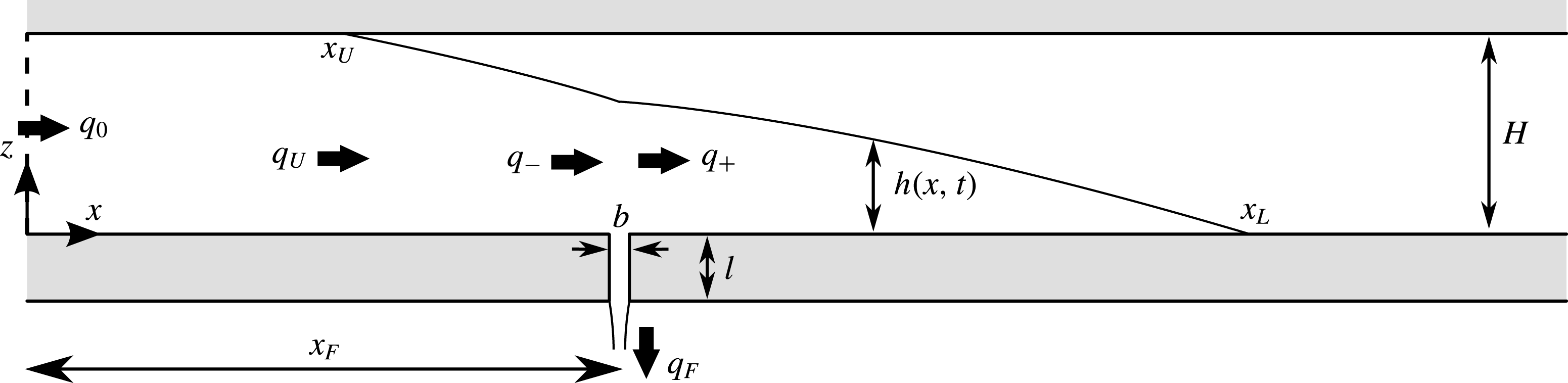
(see figure 1). Two horizontal impermeable boundaries along
 $z=0$
and
 $z=H$
are assumed to confine the medium vertically into a layer. The lower boundary contains an outlet of horizontal extent
 $b$
, vertical length
 $l$
and horizontal position centred on
 $x=x_{F}$
, through which fluid can leak. The fluid flow is modelled using Darcy’s law with momentum- and mass-continuity equations given respectively by
 $$\begin{eqnarray}\displaystyle \boldsymbol{u}=\frac{k}{{\it\mu}}(-\boldsymbol{{\rm\nabla}}p-{\it\rho}g\hat{\boldsymbol{z}})\quad \text{and}\quad \boldsymbol{{\rm\nabla}}\boldsymbol{\cdot }\boldsymbol{u}=0, & & \displaystyle\end{eqnarray}$$
where
 $\boldsymbol{u}(\boldsymbol{x},t)\equiv (u,w)$
is the Darcy velocity,
 $p(\boldsymbol{x},t)$
is the fluid pressure,
 $g$
is the gravitational acceleration and
 $\hat{\boldsymbol{z}}$
is the vertical unit vector (Bear Reference Bear1988).
Cross-section of a two-dimensional porous medium containing horizontal boundaries along
 $z=0$
and
 $H$
and an outlet centred on
 $x=x_{F}$
which allows fluid to leak from the medium.

We consider the situation where fluid invades the medium from an initially dry state. As a source condition, we impose
 $$\begin{eqnarray}\displaystyle q(0,t)=q_{0},\quad \text{where }q(x,t)\equiv \int _{0}^{h(x,t)}u(x,z,t)\,\text{d}z & & \displaystyle\end{eqnarray}$$
is the horizontal velocity integrated across the depth of the current and
 $q_{0}$
is the constant flux per unit width at which fluid is introduced at
 $x=0$
. This condition represents the introduction of fluid along a fault in a geological formation, for example.
Assuming that the current is much longer than it is tall, we neglect the viscous stresses due to vertical velocity
 $w$
in the vertical component of Darcy’s equation (2.1a
) to yield the equation describing hydrostatic pressure,
 $$\begin{eqnarray}\displaystyle \frac{\partial p}{\partial z}=-{\it\rho}g\quad \text{and hence}\quad p(\boldsymbol{x},t)=P(x,t)-{\it\rho}g[z-h(x,t)] & & \displaystyle\end{eqnarray}$$
on integration, where the constant of integration
 $P(x,t)\equiv p(x,h,t)$
is the unknown pressure along the upper interface of the current. Depending on whether the interface is a free surface or lies in contact with the upper boundary of the medium, the manner in which
 $P(x,t)$
is determined differs.
2.1. The free-surface region
Assuming that the ambient air is of negligible viscosity and density, we can approximate its pressure as a constant
 $p_{0}$
. On the free surface, continuity of stress with the ambient fluid determines the constant of integration in (2.3b
) as
 $P(x,t)=p_{0}$
, assuming negligible surface tension (with significant surface tension,
 $p_{0}$
may be better represented by the capillary entry pressure). Then (2.3b
) yields
 $$\begin{eqnarray}p(\boldsymbol{x},t)=p_{0}-{\it\rho}g[z-h(x,t)]\quad \text{if }h(x,t)<H.\end{eqnarray}$$
Using (2.4) to evaluate the pressure field in the horizontal component of Darcy’s equation (2.1a ), we obtain the horizontal velocity
 $$\begin{eqnarray}\displaystyle u=-U\frac{\partial h}{\partial x},\quad \text{where }U\equiv \frac{{\it\rho}gk}{{\it\mu}} & & \displaystyle\end{eqnarray}$$
is the velocity scale associated with purely vertical gravity-driven flow in a porous medium. Equation (2.5a
) shows that the horizontal velocity
 $u=u(x,t)$
is independent of the vertical coordinate
 $z$
and is proportional to the free-surface slope
 $\partial h/\partial x$
. To determine the evolution of the free surface
 $h(x,t)$
, we use the depth-integrated form of the continuity equation (2.1b
) given by
 $$\begin{eqnarray}\displaystyle {\it\phi}\frac{\partial h}{\partial t}=-\frac{\partial q}{\partial x},\quad \text{where }q=-Uh\frac{\partial h}{\partial x} & & \displaystyle\end{eqnarray}$$
is the flux per unit width, obtained by substituting (2.5a
) into (2.2b
). Using (2.6b
) to evaluate
 $q$
in (2.6a
), we obtain the governing nonlinear diffusion equation
 $$\begin{eqnarray}{\it\phi}\frac{\partial h}{\partial t}=U\frac{\partial }{\partial x}\left(h\frac{\partial h}{\partial x}\right).\end{eqnarray}$$
At the front
 $x=x_{L}(t)$
, we impose the conditions of vanishing thickness and flux,
 $$\begin{eqnarray}\displaystyle h(x_{L},t)=0\quad \text{and}\quad q(x_{L},t)=0. & & \displaystyle\end{eqnarray}$$
By suitably combining (2.8a,b ) (see appendix A), the frontal rate of propagation can be determined as equal to the interstitial flow rate, and hence
 $$\begin{eqnarray}{\it\phi}{\dot{x}}_{L}=u(x_{L},t)=-U\frac{\partial h}{\partial x}(x_{L},t),\end{eqnarray}$$
where we have used (2.5a
) to evaluate
 $u$
.
If the free surface lies below the upper boundary at the input (
 $h(0,t)<H$
), we can combine (2.2a
) and (2.6b
) to yield the boundary condition
 $$\begin{eqnarray}q(0,t)=-Uh(0,t)\frac{\partial h}{\partial x}(0,t)=q_{0}\quad \text{if }h(0,t)<H.\end{eqnarray}$$
Note that (2.10) is only applicable before the current makes contact with the upper boundary (
 $h(0,t)<H$
).
If the current contains a component lying downstream of the outlet (
 $x_{F}<x_{L}$
), then we impose the conditions of continuity on the height and flux between the regions just upstream and downstream of the outlet given by
 $$\begin{eqnarray}\displaystyle h_{+}=h_{-}\quad \text{and}\quad q_{+}=q_{-}-q_{F}(t), & & \displaystyle\end{eqnarray}$$
where the
 $\pm$
subscripts represent quantities just downstream and just upstream of the outlet,
 $q$
is given by (2.6b
) and
 $q_{F}(t)$
is the leakage rate through the outlet, to be determined in § 2.3.
2.2. The depth-filled region
If the current lies in contact with the upper boundary, as illustrated in figures 1 and 2(b), then it forms two regions separated by a second contact line on
 $x=x_{U}(t)$
. The two regions are referred to as the downstream free-surface region,
 $x_{U}<x<x_{L}$
, wherein
 $h<H$
, and the depth-filled region,
 $0\leqslant x\leqslant x_{U}$
, wherein
 $h=H$
.
The three possible flow configurations of the current: (a) it lies completely detached from the top boundary (
 $h(0,t)<H$
); (b) it contains a region wherein the current fills the depth of the medium upstream of the outlet (
 $h(0,t)<H$
but
 $h(x_{F},t)<H$
); or (c) the depth-filled region contains the outlet and the entire free surface lies downstream of the outlet (
 $h(x_{F},t)=H$
).

The expression for the flux in the free-surface region (2.6b
) does not apply in the depth-filled region because the condition of pressure continuity used to evaluate
 $P(x,t)$
and obtain (2.4) is unavailable. Instead, we determine the flow rate in the depth-filled region by noting that the uniformity of the height of the current in that region
 $(h=H)$
implies that the flux per unit width is horizontally uniform,
 $$\begin{eqnarray}\frac{\partial q}{\partial x}=0\quad \text{in }0<x<x_{U}(t),\end{eqnarray}$$
in accord with (2.6a
). If the upper contact line lies upstream of the outlet (
 $x_{U}<x_{F}$
), as shown in figure 2(b), an integration of (2.12) subject to (2.2a
) implies that the flux through the depth-filled region is simply equal to the injection flux,
 $$\begin{eqnarray}q=q_{0}\quad \text{in }0<x<x_{U}\quad \text{if }x_{U}<x_{F}.\end{eqnarray}$$
If instead the outlet lies in the interior of the depth-filled region, as illustrated in figure 2(c), then (2.2a ) together with (2.11b ) implies that
 $$\begin{eqnarray}q=\left\{\begin{array}{@{}ll@{}}q_{0}\quad & \text{in }0<x<x_{F}\\ q_{+}(t)=q_{0}-q_{F}(t)\quad & \text{in }x_{F}<x<x_{U}\end{array}\right.\quad \text{if }x_{U}>x_{F}.\end{eqnarray}$$
In formulating the leakage rate
 $q_{F}(t)$
in § 2.3 we will need the pressure field
 $p(\boldsymbol{x},t)$
associated with the flow fields (2.13) and (2.14). To calculate this, we use the horizontal component of Darcy’s equation (2.1a
) which, when rearranged in favour of the pressure gradient, is given by
 $$\begin{eqnarray}\frac{\partial p}{\partial x}=-\frac{{\it\mu}u}{k}=-\frac{{\it\mu}q}{kH}\quad \text{in }0<x<x_{U},\end{eqnarray}$$
where
 $q=Hu$
is the (piecewise uniform) flux per unit width given by (2.13) if
 $x_{U}<x_{F}$
and (2.14) otherwise. In the former case, an integration of (2.15), followed by a comparison with (2.3b
) and use of the continuity condition
 $p(x_{U},H,t)=p_{0}$
, determines the pressure field as
 $$\begin{eqnarray}p(\boldsymbol{x},t)=p_{0}+{\it\rho}g(H-z)+\frac{{\it\mu}q_{0}}{k}[x_{U}(t)-x].\end{eqnarray}$$
With
 $q$
given instead by (2.14), we obtain the conditional relationship
 $$\begin{eqnarray}p(\boldsymbol{x},t)=\left\{\begin{array}{@{}ll@{}}p_{0}+{\it\rho}g(H-z)+\displaystyle \frac{\displaystyle {\it\mu}}{\displaystyle k}\{q_{+}(t)[x_{U}(t)-x_{F}]+q_{0}[x_{F}-x]\} & \text{in }0<x<x_{F},\\ p_{0}+{\it\rho}g(H-z)+\displaystyle \frac{\displaystyle {\it\mu}}{\displaystyle k}q_{+}(t)[x_{U}(t)-x] & \text{in }x_{F}<x<x_{U},\end{array}\right.\end{eqnarray}$$
where
 $q_{+}(t)\equiv q_{0}-q_{F}(t)$
is the retained flux given in (2.14).
When the current lies in contact with the upper boundary,
 $h(0,t)=H$
, (2.10) cannot be applied because the free surface lies downstream of
 $x=0$
. Instead, we impose the condition of flux continuity at the upper contact line given by
 $$\begin{eqnarray}-\!UH\frac{\partial h}{\partial x}(x_{U},t)=\left\{\begin{array}{@{}ll@{}}q_{0}\quad & \text{if }x_{U}(t)<x_{F},\\ q_{0}-q_{F}(t) & \text{if }x_{U}(t)>x_{F},\end{array}\right.\end{eqnarray}$$
where the flux on the right-hand side is evaluated using (2.13) or (2.14), depending on whether the upper contact line lies upstream or downstream of the outlet.
The upper contact line at
 $x_{U}(t)$
is a freely moving boundary whose evolution must be determined. Mathematically, the condition which determines
 ${\dot{x}}_{U}(t)$
is
 $$\begin{eqnarray}h(x_{U}(t),t)=H,\end{eqnarray}$$
which states that the upper contact line lies where the free surface intersects the upper boundary. It is convenient for numerical implementation to obtain, if possible, an explicit evolution equation for the upper contact line
 ${\dot{x}}_{U}$
analogous to (2.9). Differentiation of (2.19) with respect to time yields
 $$\begin{eqnarray}{\dot{x}}_{U}=-\frac{\partial h}{\partial t}\bigg/\frac{\partial h}{\partial x}\quad \text{at }x=x_{U}^{+},\end{eqnarray}$$
which shows that the propagation of the contact line is associated with vertical thickening of the current just ahead of it. However, at this juncture the argument used in appendix A cannot be continued to develop an equation for
 ${\dot{x}}_{U}$
because the flux towards the upper contact line
 $q(x_{U},t)$
does not vanish in accord with (2.18). The same difficulty arises in modelling the contact line that separates a floating and grounded component of a gravity current in a Hele-Shaw cell (Pegler et al.
Reference Pegler, Kowal, Hasenclever and Worster2013). To evaluate the right-hand side of (2.20) numerically, we utilize the same method of Pegler et al. (Reference Pegler, Kowal, Hasenclever and Worster2013), whereby
 $\partial h/\partial t$
is calculated using the result of a trial integration step under an artificial imposition of
 ${\dot{x}}_{U}=0$
. The predicted penetration of the current through the top boundary
 ${\it\delta}h=h-H$
arising from this trial is then used to evaluate the rate of propagation (2.20) as
 $$\begin{eqnarray}{\dot{x}}_{U}=-\frac{{\it\delta}h}{{\it\delta}t}\bigg/\frac{\partial h}{\partial x},\end{eqnarray}$$
where
 ${\it\delta}t$
is the time step. It is notable that the difficulty described above does not arise in studies where ambient fluid viscosity is included (Pegler et al.
Reference Pegler, Huppert and Neufeld2014a
). In that case, conditions of vanishing thickness and flux of the ambient fluid at the contact line can be utilized to obtain an evolution equation describing its rate of propagation (given by (2.8b) in Pegler et al.
Reference Pegler, Huppert and Neufeld2014a
) using an analogous argument to that given in appendix A. The break-down of that equation as the ambient viscosity tends to zero occurs because the Darcy’s law used to describe the ambient flow is degenerate in that singular limit.
2.3. The leakage law
It is assumed that the flow rate through the outlet is related to the applied pressure gradient across it according to Darcy’s law, which implies that
 $$\begin{eqnarray}\displaystyle q_{F}(t)=\frac{bk_{F}}{{\it\mu}l}[p(x_{F},0,t)-p_{0}+{\it\rho}gl], & & \displaystyle\end{eqnarray}$$
where
 $k_{F}$
is the permeability of the outlet. The first two terms in (2.22) represent the pressure difference between the top and bottom of the outlet. The third term represents the added driving force due to gravity acting on fluid along the interior of the outlet.
Using (2.4) to evaluate
 $p(x_{F},0,t)$
in (2.22) if
 $h(x_{F},t)<H$
and (2.14) if
 $h(x_{F},t)=H$
, we obtain the conditional leakage law given by
 $$\begin{eqnarray}\displaystyle q_{F}(t)=\left\{\begin{array}{@{}ll@{}}\displaystyle \frac{\displaystyle b{\it\rho}gk_{F}}{\displaystyle l{\it\mu}}(h(x_{F},t)+l) & \text{if }h(x_{F},t)<H,\\ \displaystyle \frac{\displaystyle bk_{F}}{\displaystyle l{\it\mu}}\left\{{\it\rho}g(H+l)+\displaystyle \frac{\displaystyle {\it\mu}}{\displaystyle kH}[x_{U}(t)-x_{F}][q_{0}-q_{F}(t)]\right\} & \text{if }h(x_{F},t)=H.\end{array}\right. & & \displaystyle\end{eqnarray}$$
Note that the right-hand side of (2.23b
) is itself dependent on
 $q_{F}(t)$
because the contribution to leakage due to back-pressure is linearly proportional to the flux it drives,
 $q_{0}-q_{F}(t)$
. Making
 $q_{F}(t)$
the subject of (2.23b
), we obtain finally
 $$\begin{eqnarray}\displaystyle q_{F}(t)=\widetilde{q}_{F}(t)\equiv \left\{\begin{array}{@{}ll@{}}\displaystyle \frac{\displaystyle b{\it\rho}gk_{F}}{\displaystyle {\it\mu}l}[h(x_{F},t)+l] & \text{if }h(x_{F},t)<H,\\ \displaystyle \frac{\displaystyle bk_{F}}{\displaystyle {\it\mu}l}\left[\displaystyle \frac{\displaystyle {\it\rho}g(H+l)+\displaystyle \frac{\displaystyle {\it\mu}q_{0}}{\displaystyle kH}[x_{U}(t)-x_{F}]}{\displaystyle 1+\displaystyle \frac{\displaystyle bk_{F}}{\displaystyle lkH}[x_{U}(t)-x_{F}]}\right] & \text{if }h(x_{F},t)=H.\end{array}\right. & & \displaystyle\end{eqnarray}$$
While the flow is detached from the upper boundary above the outlet (
 $h(x_{F},t)<H$
), (2.24a
) implies that leakage rate is linearly related to the hydrostatic head
 $h(x_{F},t)$
. This is the equivalent leakage rate applicable at all times in a deep porous medium (Pritchard et al.
Reference Pritchard, Woods and Hogg2001). If the current instead fills the full depth of the medium above the outlet (
 $h(x_{F},t)=H$
) then the leakage law switches to (2.24b
). The contribution to leakage due to the hydrostatic head is then fixed at a constant, but there is a new contribution due to the back-pressure associated with driving fluid downstream. The emergent back-pressure depends on the length of the depth-filled region downstream of the outlet,
 $x_{U}(t)-x_{F}$
. This feature is absent in the study of Pegler et al. (Reference Pegler, Huppert and Neufeld2014b
), where the dominance of back-pressure generated by long-range mobilization of ambient fluid causes the leakage rate to become effectively fixed once
 $h(x_{F},t)=H$
. Importantly, the back-pressure generated by the invading fluid in the present context will be shown to increase leakage rates significantly over time.
Before the current reaches the outlet, there is no accumulation of fluid above it (
 $h(x_{F},t)=0$
). Equation (2.24a
) then predicts that leakage occurs at a rate
 $q_{min}\equiv bk_{F}U/k$
owing to the effect of gravity acting on fluid filling the interior of the outlet. The leakage rate predicted by (2.24) is then unphysical because there is no fluid above the outlet to draw. This inconsistency arises because of the assumption made initially in (2.22) that the outlet is always filled with fluid. Generally, this assumption is invalid if the current delivers a smaller flux towards the outlet than is predicted to leak according to (2.24). We accommodate this by assuming that, if the rate at which fluid flows towards the outlet
 $q_{-}$
is less than the minimum leakage flux associated with a fluid-filled outlet
 $q_{min}$
, then all fluid reaching the outlet leaks through it. Therefore, we impose
 $$\begin{eqnarray}q_{F}=\left\{\begin{array}{@{}ll@{}}q_{-} & \text{if }q_{-}<q_{min}\equiv bk_{F}U/k,\\ \widetilde{q}_{F} & \text{if }q_{-}>q_{min},\end{array}\right.\end{eqnarray}$$
where
 $\widetilde{q}_{F}$
is the rate given by (2.24). Only once the flux per unit width of fluid flowing towards the outlet satisfies
 $q_{-}>q_{min}$
does accumulation above the outlet (
 $h(x_{F},t)>0$
) occur consistently with (2.24).
2.4. The significance of ambient back-pressure
The pressure fields given by (2.4), (2.16) and (2.17) were calculated under the assumption that ambient viscosity is negligible. This is opposite to the assumption made by Pegler et al. (Reference Pegler, Huppert and Neufeld2014b ), who considered situations where the ambient contribution to the back-pressure is dominant over any perturbation to it due to the presence of the invading fluid. The situations for which these two different assumptions are applicable can be catalogued by the dimensionless parameter
 $$\begin{eqnarray}A\equiv \frac{{\it\mu}_{a}}{{\it\mu}}\frac{L}{x_{U}},\end{eqnarray}$$
where
 ${\it\mu}_{a}$
is the viscosity of an ambient fluid,
 $x_{U}$
is the characteristic extent of the current and
 $L$
is the length scale over which the ambient fluid is mobilized (see the discussion surrounding (2.13) in Pegler et al.
Reference Pegler, Huppert and Neufeld2014b
). The parameter
 $A$
represents the ratio of the contributions to the back-pressure arising from the long-range mobilization of the ambient fluid along the length of the medium to that arising from the current. In taking a uniform reference pressure in obtaining (2.4), (2.16) and (2.17), it was assumed that the latter is negligible and hence
 $A\ll 1$
. Pegler et al. (Reference Pegler, Huppert and Neufeld2014b
) assumed instead that the back-pressure is dominated by the contribution due to ambient fluid, for which
 $A\gg 1$
. The parameter settings for the different modelling assumptions are thus summarized by
 $$\begin{eqnarray}\displaystyle \begin{array}{@{}l@{}}A\gg 1\quad \text{and}\quad {\it\mu}_{a}/{\it\mu}=\text{any value (Pegler et al. 2014b)}\\ A\ll 1\quad \text{and}\quad {\it\mu}_{a}/{\it\mu}\ll 1~\text{(present study)}.\end{array} & & \displaystyle\end{eqnarray}$$
Note that there are two different dynamical respects in which the ambient viscosity can be considered significant: one, measured by
 ${\it\mu}_{a}/{\it\mu}$
, is its effect on local flow dynamics; the other, measured by
 $A$
, is its effect on back-pressure. For illustration, we note that the settings
 ${\it\mu}_{a}/{\it\mu}\ll 1$
but
 $A\gg 1$
give the unusual situation in which the ambient viscosity can be neglected in the local flow dynamics but is dominant in the determination of the back-pressure. This is a special limiting case of the situations considered by Pegler et al. (Reference Pegler, Huppert and Neufeld2014b
). The case
 ${\it\mu}_{a}/{\it\mu}\ll 1$
and
 $A\ll 1$
considered in this paper corresponds to the different situation in which ambient viscosity is negligible in all respects, resulting in the new mathematical feature of a time-dependent back-pressure in (2.24). In this regard, the situations considered here differ fundamentally from those of Pegler et al. (Reference Pegler, Huppert and Neufeld2014b
).
For the invasion of water into an air-filled porous medium,
 ${\it\mu}_{a}/{\it\mu}\approx 0.01$
and hence we can form the illustrative estimate
 $A\approx 0.01L/x_{U}$
. With
 $x_{U}=O(L)$
, it is thus found that
 $A\ll 1$
and hence that the contribution to the back-pressure due to the ambient air is negligible. The assumption of a constant ambient pressure
 $p_{0}$
used in the calculation of the pressure fields (2.4), (2.16) and (2.17) is therefore reasonable in this application. The situation relevant to geological CO
 $_{2}$
storage is very different because the ambient saline is at least an order of magnitude more viscous than the injected CO
 $_{2}$
. Typical values of the viscosity ratio
 ${\it\mu}_{a}/{\it\mu}\approx 10$
–100 imply that
 $A>10(L/x_{L})$
. Given also that
 $x_{U}<L$
, we find that
 $A>10$
is at least one order of magnitude larger than unity. With the added realistic assumption that the ambient fluid comprises the majority of fluid in the aquifer,
 $x_{U}\ll L$
and
 $A\gg 10$
is yet larger. This indicates that the ambient flow is likely to dominate the determination of back-pressure in the context of geological CO
 $_{2}$
storage, for which the situations considered by Pegler et al. (Reference Pegler, Huppert and Neufeld2014b
) are therefore more relevant.
3. Theoretical analysis
We make the system given by (2.7)–(2.9) and (2.24)–(2.25) dimensionless by defining the scaled variables
 $$\begin{eqnarray}x\equiv \frac{UH^{2}}{q_{0}}\hat{x},\quad t\equiv \frac{{\it\phi}UH^{3}}{q_{0}^{2}}\hat{t},\quad h\equiv H{\hat{h}},\quad q\equiv q_{0}\hat{q}.\end{eqnarray}$$
The horizontal length and time scales in (3.1) are representative of the time and extent at which a gravity current introduced at a constant rate
 $q_{0}$
into a two-dimensional porous medium attains the depth of the medium
 $H$
. On dropping hats, the free-surface evolution equation (2.7) becomes
 $$\begin{eqnarray}\frac{\partial h}{\partial t}=\frac{\partial }{\partial x}\left(h\frac{\partial h}{\partial x}\right).\end{eqnarray}$$
The frontal height condition (2.8a ) and evolution equation (2.9) become
 $$\begin{eqnarray}\displaystyle h(x_{L},t)=0,\quad {\dot{x}}_{L}=-\frac{\partial h}{\partial x}(x_{L},t). & & \displaystyle\end{eqnarray}$$
The input condition relevant before the current makes contact with the upper boundary (2.10) becomes
 $$\begin{eqnarray}-\!h(0,t)\frac{\partial h}{\partial x}(0,t)=1\quad \text{if }h(0,t)<1.\end{eqnarray}$$
The conditions (2.18) and (2.19) at the upper contact line, applicable once contact is made with the upper boundary, become
 $$\begin{eqnarray}\displaystyle \left.\begin{array}{@{}rl@{}}h(x_{U},t)\, & =1,\\ \displaystyle -\frac{\partial h}{\partial x}(x_{U},t)\, & =\left\{\begin{array}{@{}ll@{}}1 & \text{if }x_{U}<X,\\ 1-q_{F}(t) & \text{if }x_{U}>X.\end{array}\right.\end{array}\right\}\quad \text{if }h(0,t)=1. & & \displaystyle\end{eqnarray}$$
Finally, the leakage law given by combining (2.24) and (2.25) becomes
 $$\begin{eqnarray}\displaystyle q_{F}(t)=\left\{\begin{array}{@{}ll@{}}q_{-}(t) & \text{if }h(X,t)=0\quad \text{and}\quad q_{-}(t)<Q,\\ Q+(1-Q)\displaystyle \frac{\displaystyle h(X,t)}{\displaystyle D} & \text{if }0<h(X,t)<1,\\ 1-\displaystyle \frac{\displaystyle D-1}{\displaystyle D/(1-Q)+[x_{U}(t)-X]} & \text{if }h(X,t)=1.\end{array}\right. & & \displaystyle\end{eqnarray}$$
The system above depends on the three dimensionless parameters
 $$\begin{eqnarray}\displaystyle X\equiv \frac{{\it\mu}q_{0}x_{F}}{{\it\rho}gkH^{2}},\quad Q\equiv \frac{q_{min}}{q_{0}}\equiv \frac{bk_{F}{\it\rho}g}{{\it\mu}q_{0}},\quad D\equiv \frac{l}{H}\left(\frac{1}{Q}-1\right). & & \displaystyle\end{eqnarray}$$
These represent the dimensionless outlet position
 $X$
, the ratio of the threshold leakage rate to the injection rate
 $Q$
, and the hydrostatic parameter
 $D$
which, when positive, represents the ratio of the hydrostatic head for which leakage driven by gravity alone balances the injection rate, to the depth of the medium. This definition is consistent with (3.6b
), which implies that
 $q_{F}=1$
if
 $h=D$
. With
 $D<0$
, the injection rate
 $q_{0}$
is less than the threshold
 $q_{min}$
defined in (2.25). This occurs only if
 $Q>1$
in accord with (3.7c
), implying that the parameter settings
 $D<0$
and
 $Q>1$
must go together. In such situations, the leakage driven by gravity along the length of the outlet alone is sufficient to match the injection rate without the need for any accumulation of fluid above the outlet. With
 $0<D<1$
, the hydrostatic head required for gravity-driven leakage to balance the injection rate lies in the interior of the medium. With
 $D>1$
, it lies higher than the upper boundary. Therefore, leakage driven by gravity alone cannot balance the injection rate.
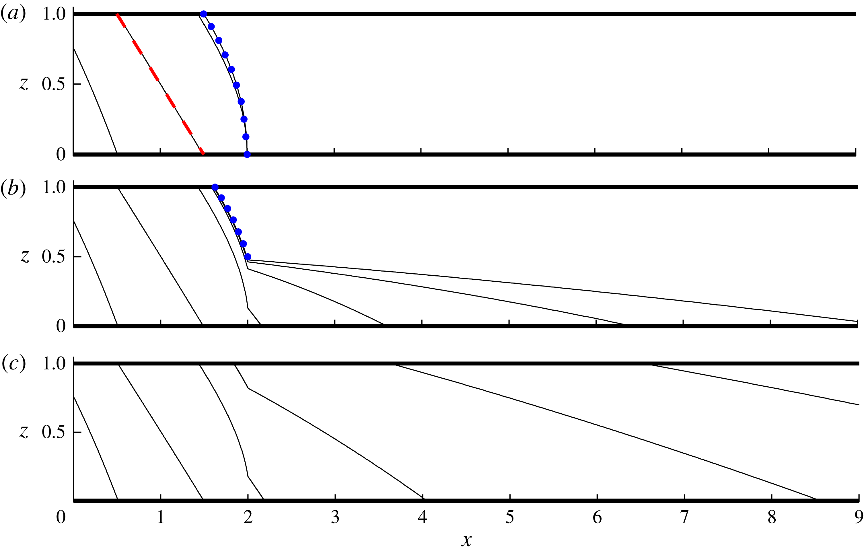
Numerically determined solutions (solid curves) for (a) any
 $D<0$
and
 $Q>1$
, (b)
 $D=0.5$
and
 $Q=0.5$
, and (c)
 $D=2$
and
 $Q=0.5$
, all with outlet position
 $X=2$
, shown at
 $t=0.2,1,2,5,20$
and
 $50$
. The steady states given by (3.9) and (3.11) are shown as dotted curves (blue online) in (a,b), respectively.

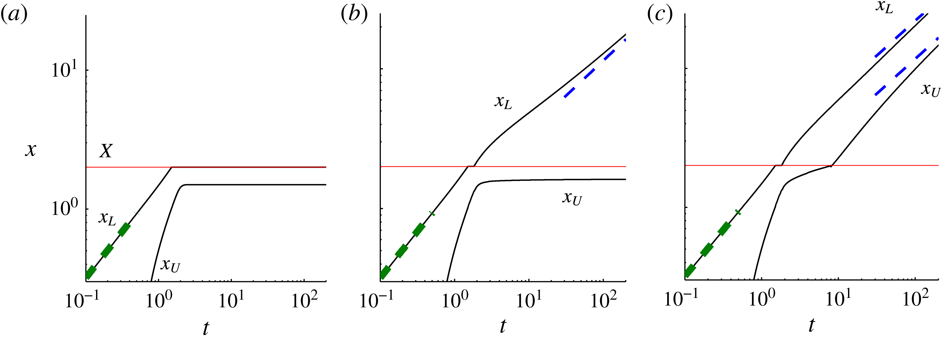
(a–c) The contact-line positions
 $x_{L}(t)$
and
 $x_{U}(t)$
for (a) any
 $D<0$
and
 $Q>1$
, (b)
 $D=0.5$
and
 $Q=0.5$
, and (c)
 $D=2$
and
 $Q=0.5$
. The horizontal lines (red online) indicate the outlet position
 $X=2$
. The early-time evolution of the frontal contact line
 $x_{L}=1.48\,t^{2/3}$
is shown as a thick dashed line (green online) in each panel. The long-term asymptotic positions determined in § 3.3 are shown as thin dashed lines (blue online) in (b,c).

Three illustrative numerical solutions to (3.2)–(3.6) are shown in figure 3 for (a) any
 $D<0$
and
 $Q>1$
, (b)
 $D=0.5$
and
 $Q=0.5$
, and (c)
 $D=2$
and
 $Q=0.5$
, each with the dimensionless outlet position
 $X=2$
. The numerical solutions were obtained using a second-order finite-difference scheme in which the regions upstream and downstream of the outlet are transformed onto fixed numerical domains. Once formed, the upper contact line
 $x_{U}(t)$
was propagated by employing trial integration steps with a stationary upper contact line
 ${\dot{x}}_{U}=0$
, as described in the final paragraph of § 2.1.
The three illustrative numerical examples reveal three different long-term regimes of flow. If
 $D<0$
, all the invading fluid leaks directly through the outlet and no fluid propagates downstream of it. If
 $0<D<1$
, some fluid propagates downstream of the outlet but the free surface in that region remains detached from the upper boundary for all time. If
 $D>1$
, the current fills the full depth of the medium above the outlet and the free surface advances indefinitely downstream.
3.1. Flow regimes preceding leakage
The dimensionless parameters in the system
 $X,Q$
and
 $D$
all relate to leakage. Therefore, the dimensionless solutions are all equivalent before any contact with the outlet occurs, that is, while
 $x_{L}(t)<X$
. During this time, the flow evolves as a gravity current injected at a constant rate into a confined porous medium, corresponding to the limiting case of zero ambient fluid viscosity in the analysis of Pegler et al. (Reference Pegler, Huppert and Neufeld2014a
). Initially, while the current lies below the upper boundary, the evolution is the same as a gravity current injected into a porous medium without an upper boundary, which is described by a similarity solution of horizontal and vertical extents
 $x_{L}=1.482\,t^{2/3}$
and
 $h(0,t)=1.296\,t^{1/3}$
, respectively (Huppert & Woods Reference Huppert and Woods1995). The first of these is plotted as a thick dashed line (green online) in each panel of figure 4, where it is seen to match our numerically determined evolution of
 $x_{L}$
at early times.
If the outlet lies sufficiently far downstream of the input (specifically if
 $X>0.882$
), then the current will make contact with the upper boundary before it reaches the outlet. By setting
 $h(0,t)=1.296\,t^{1/3}=1$
, the time of first contact between the fluid and the upper boundary is determined as
 $t\approx 0.459$
. The solution after this time adjusts relatively quickly towards an asymptotic solution obtained by Pegler et al. (Reference Pegler, Huppert and Neufeld2014b
) as
 $$\begin{eqnarray}h\sim x_{L}-x,\quad x_{U}\sim t-{\textstyle \frac{1}{2}},\quad x_{L}\sim t+{\textstyle \frac{1}{2}}\quad (t\gtrsim 1\text{ but }x_{L}(t)<X),\end{eqnarray}$$
which describes a linear height profile of constant slope that translates horizontally with unit speed. The asymptotic solution (3.8) is shown as a dashed line (red online) in figure 3(a) at
 $t=1$
, where it is seen to match our numerically obtained solution closely.
3.2. Transient evolution
Once the current reaches the outlet (
 $x_{L}(t)=X$
), the rate at which fluid flows towards the outlet
 $q_{-}$
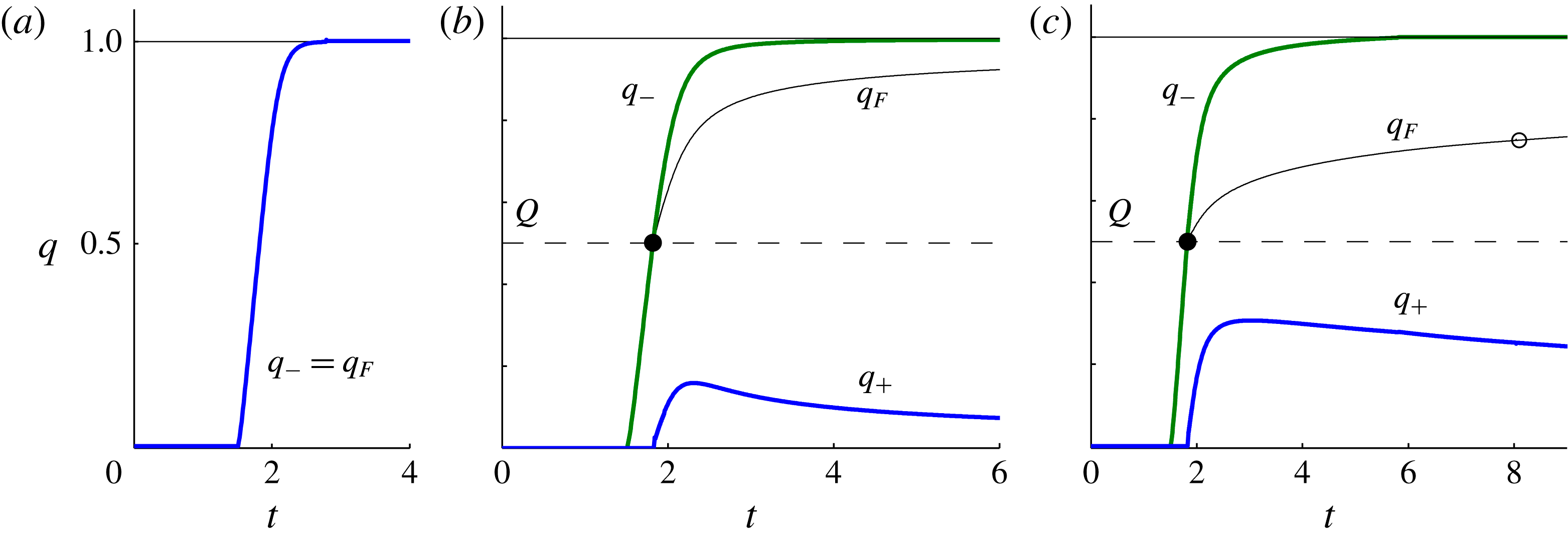
begins to increase from zero, as illustrated for our three examples in figure 5(a–c). With a non-zero threshold flux
 $Q$
, there is an interval of time during which the flux flowing towards the outlet is less than the threshold needed to accumulate fluid above it (
 $q_{-}<Q$
), and hence all the fluid reaching the outlet initially leaks in accord with (3.6a
). During this interval, the front is pinned at the outlet, as illustrated by the examples with
 $Q=0.5$
in figures 4(b,c).
The dimensionless leakage rate,
 $q_{F}(t)$
(black), flux towards the outlet
 $q_{-}(t)$
(green online), and flux flowing downstream of the outlet
 $q_{+}(t)$
(blue online), for the three numerical examples (a) any
 $D<0$
and
 $Q>1$
, (b)
 $D=0.5$
and
 $Q=0.5$
, and (c)
 $D=2$
and
 $Q=0.5$
, all with
 $X=2$
. The injection rate
 $q=1$
and threshold flux
 $q=Q$
are represented by a solid and dashed horizontal line, respectively. While
 $q_{-}<Q$
, all fluid reaching the outlet leaks through it. Once
 $q_{-}>Q$
, a residual flux
 $q_{-}-q_{F}=q_{+}>0$
feeds the component of the current downstream of the outlet. The time at which the leakage law transitions from purely gravitational leakage (3.6b
) to leakage with pressure build-up (3.6c
) is indicated by an open circle in (c).

When
 $D<0$
and
 $Q>1$
, shown in figure 3(a), the threshold leakage rate exceeds the flux of injection. The threshold flux is therefore never exceeded and all fluid leaks directly though the outlet for all time, as illustrated in figure 3(a). In that example, the rate of leakage matches the injection flux
 $q_{F}\approx 1$
to within 1 % by
 $t=3$
, as indicated in figure 5(a). The free surface is observed to approach a steady profile (cf. Pritchard et al.
Reference Pritchard, Woods and Hogg2001; Pritchard Reference Pritchard2007; Neufeld et al.
Reference Neufeld, Vella and Huppert2009; Hesse & Woods Reference Hesse and Woods2010). This profile can be determined analytically by integrating the steady form of (3.2) subject to the input condition (3.5b
) and the condition of vanishing thickness
 $h(X,t)=0$
to give
 $$\begin{eqnarray}h\sim [2(X-x)]^{1/2}\quad (t\rightarrow \infty ),\end{eqnarray}$$
which is plotted as a dotted curve (blue online) in figure 3(a). Setting
 $h=1$
in (3.9), the asymptotic position of the upper contact line is determined as
 $x_{U}\sim X-1/2$
, assuming that
 $X>1/2$
. If
 $X<1/2$
then the current remains detached from the upper boundary for all time.
With
 $D=0.5$
and
 $Q=0.5$
, the threshold flux is less than the injection rate (
 $Q<1$
). In this case, the front of the current is only temporarily pinned at the outlet, as illustrated in figures 3(b) and 4(b). The threshold flux is attained (
 $q_{-}=Q$
) at a time
 $t\approx 1.8$
, indicated by a filled circle in figure 5(b). The residual between the rate at which fluid flows towards the outlet and the rate at which it leaks,
 $q_{+}=q_{-}-q_{F}$
, then introduces fluid downstream of the outlet. Eventually, the height of the current above the outlet approaches the hydrostatic parameter
 $$\begin{eqnarray}h\sim D\quad (t\rightarrow \infty )\end{eqnarray}$$
and, consistent with (3.6b
), the leakage flux
 $q_{F}\rightarrow 1$
and the retained flux
 $q_{+}=q_{-}-q_{F}\rightarrow 0$
. The leakage rate therefore balances the injection rate asymptotically in an equivalent manner to that identified previously in the context of infinitely deep porous media (Pritchard et al.
Reference Pritchard, Woods and Hogg2001). Like the case
 $D<0$
, the free surface upstream of the outlet approaches a steady state. By integrating the steady form of (2.6a
) subject to (3.10), we obtain the steady-state height profile
 $$\begin{eqnarray}h\sim [D^{2}+2(X-x)]^{1/2},\end{eqnarray}$$
which is plotted as a dotted curve (blue online) in figure 3(b). Setting
 $h=1$
in (3.11), we determine the asymptotic position of the upper contact line
 $x_{U}\sim X-(1-D^{2})/2$
. If
 $X<(1-D^{2})/2$
then the current remains detached from the upper boundary.
When
 $D>1$
, the current eventually fills the entire depth of the medium above the outlet, as illustrated by our solution with
 $D=2$
in figure 3(c). The time at which this occurs,
 $t\approx 8$
, is indicated by an open circle in figure 5(c). At this critical time, the leakage law (3.6) switches from the second condition to the third. Leakage due to gravity then becomes fixed at a constant rate but
 $q_{F}(t)$
continues to increase owing to the build-up of back-pressure between the upper contact line and the outlet. The back-pressure increases with growth of the downstream current, and hence the retained flux flowing downstream of the outlet
 $q_{+}(t)$
decays to long times (see figure 5
c).
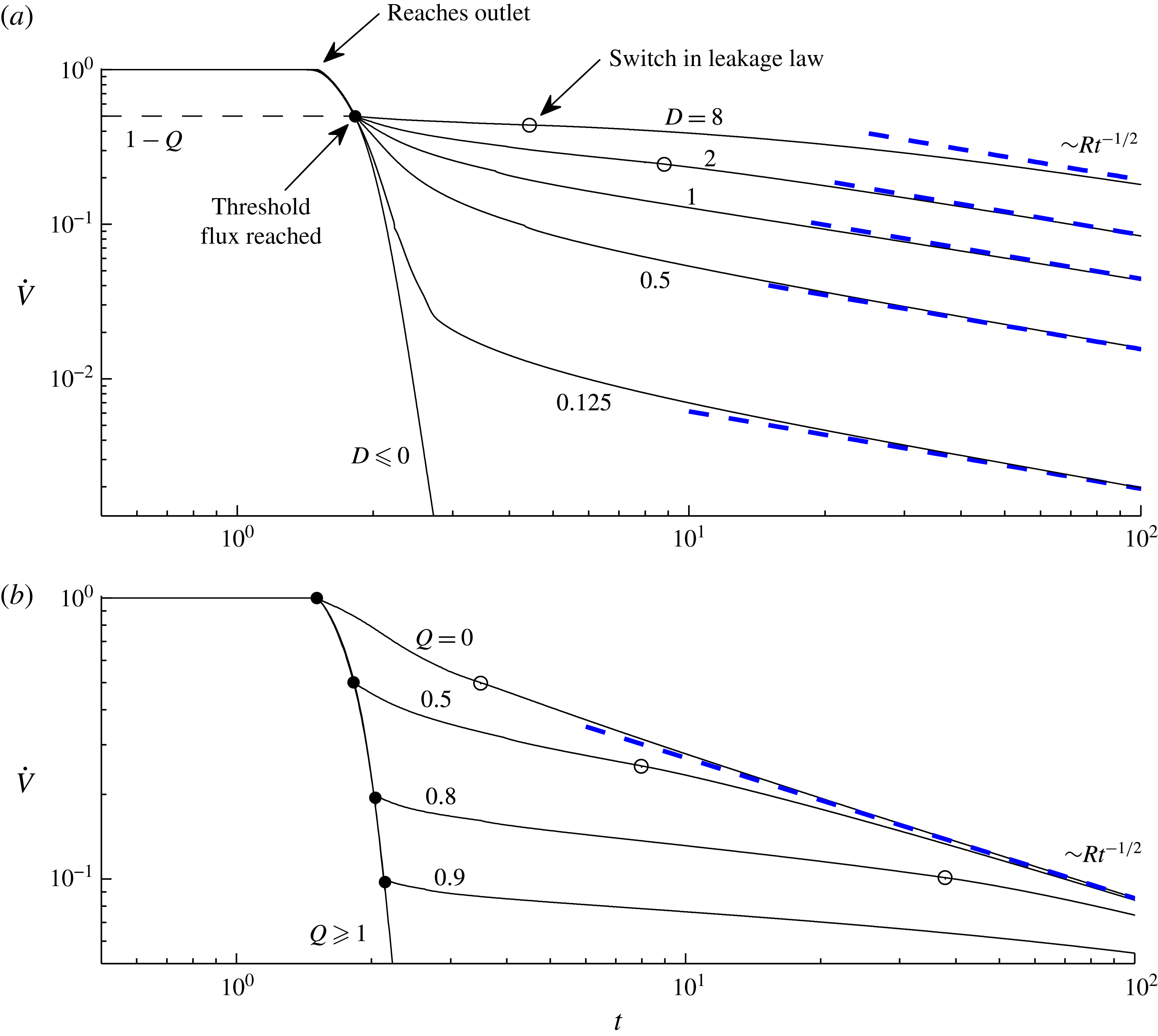
In understanding how fluid disperses underground, an important quantity is the ratio of fluid retained in a layer compared to that which migrates vertically from it to another level in the formation. This can be measured using the dimensionless rate of change of the volume of the current, given by
 $$\begin{eqnarray}\displaystyle \dot{V}(t)\equiv 1-q_{F}(t),\quad \text{where }V(t)=\int _{0}^{x_{L}(t)}h(x,t)\,\text{d}x & & \displaystyle\end{eqnarray}$$
is the total volume of the current and we have used a dot to denote
 $\text{d}/\text{d}t$
. The evolution of
 $\dot{V}(t)$
is potted as a function of time for various hydrostatic parameters
 $D$
in figure 6(a) and various threshold fluxes
 $Q$
in figure 6(b). The illustrative fracture position
 $X=2$
is chosen in all cases (variation of
 $X$
only changes the time when the asymptotic solution (3.8) reaches the outlet, so we have omitted a detailed consideration of its variation). Before the current reaches the outlet (
 $t<0.88$
),
 $\dot{V}$
is initially unity because no leakage occurs during that time (
 $q_{F}=0$
). Following the initiation of leakage, there is a sharp reduction in
 $\dot{V}$
. Once the threshold
 $q_{-}=Q$
is attained,
 $\dot{V}$
continues to decrease, before approaching a milder asymptotic rate of decay at long times. The asymptotes for
 $\dot{V}$
(shown as dashed lines, blue online), to be determined in § 3.3, increase with
 $D$
because the outlet permeability is larger in these cases (see (3.7)). The plot of figure 6(b) shows that the asymptotic volume change
 $\dot{V}$
is independent of
 $Q$
, which therefore only affects the transient evolution. However, the time scales on which the current spans the depth of the medium and subsequently approaches the asymptotic flow vary significantly with
 $Q$
.
3.3. Long-term flow regimes
Our numerical solutions indicated three distinct long-term regimes of flow dependent on whether
 $D<0$
,
 $0<D<1$
or
 $D>1$
. We refer to these as regimes
 $\text{A}$
,
 $\text{B}$
and
 $\text{C}$
, respectively. Regime
 $\text{A}$
arises when fluid flows directly through the leakage pathway, occurring if
 $D<0$
. In this case, the long-term asymptotic flow is described entirely by the steady state (3.9). Regime
 $\text{B}$
arises when the current remains detached from the upper boundary and the asymptotic condition (3.10) is applicable, occurring if
 $0<D<1$
. Finally, regime
 $\text{C}$
arises if the free surface contacts the upper boundary above the outlet, occurring if
 $D>1$
. The long-term flow is then subject to the alternative asymptotic condition
 $x_{U}(t)\rightarrow \infty$
.
The rate of change of the dimensionless volume of fluid in the medium
 $\dot{V}$
defined by (3.12) plotted as a function of time. In (a), solutions are shown for a selection of hydrostatic parameters
 $D=0.125{-}8$
and
 $D\leqslant 0$
with the dimensionless threshold flux
 $Q=0.5$
and outlet position
 $X=2$
fixed. In (b), solutions are shown for a selection of dimensionless threshold fluxes
 $Q=0{-}0.9$
and
 $Q\geqslant 1$
, all with fixed
 $D=2$
and
 $X=2$
. The time at which the threshold flux is reached, occurring when
 $q_{-}=Q$
and
 $\dot{V}=1-Q$
, at which the leakage law switches from (3.6a
) to (3.6b
) and fluid begins to propagate downstream of the outlet, is indicated by a filled circle. The time at which the current contacts the upper boundary directly above the outlet (
 $h(X,t)=1$
), corresponding to the switch in the leakage law from (3.6b
) to (3.6c
) for cases of
 $D>1$
, is indicated by an unfilled circle. Panel (a) illustrates the approach of
 $\dot{V}$
towards different asymptotes (3.18c
) (dashed lines, blue online), as
 $D$
varies. Panel (b) illustrates that, while the asymptotic evolution of
 $\dot{V}$
is independent of
 $Q$
, the time scales on which
 $\dot{V}$
approaches the asymptote increases significantly with
 $Q$
.

To investigate the long-term flow relevant to regime
 $\text{B}$
, we consider the solution to (3.2)–(3.6) subject to (3.10). A scaling analysis of these equations shows that there is no constant horizontal length scale associated with the flow, indicating a self-similar asymptotic regime. The relevant similarity variables are
 $$\begin{eqnarray}\displaystyle {\it\eta}=t^{-1/2}(x-X),\quad h=h({\it\eta}),\quad q_{+}=R\,t^{-1/2}, & & \displaystyle\end{eqnarray}$$
where the constant
 $R$
will be referred to as the retainment coefficient. Recasting (3.2) in terms of (3.13), we obtain
 $$\begin{eqnarray}-\!{\textstyle \frac{1}{2}}{\it\eta}h^{\prime }=(hh^{\prime })^{\prime },\end{eqnarray}$$
where we use a prime to denote
 $\text{d}/\text{d}{\it\eta}$
. The frontal conditions (3.3a,b
) become
 $$\begin{eqnarray}\displaystyle h({\it\eta}_{L})=0,\quad h^{\prime }({\it\eta}_{L})=-{\textstyle \frac{1}{2}}{\it\eta}_{L}. & & \displaystyle\end{eqnarray}$$
and the asymptotic condition (3.10) becomes
 $$\begin{eqnarray}\displaystyle h(0)=D. & & \displaystyle\end{eqnarray}$$
In terms of the rescaled similarity variables
 $\widetilde{h}=h/D$
,
 $\widetilde{{\it\eta}}=D^{1/2}{\it\eta}$
, and
 $\widetilde{R}=D^{-3/2}R$
, (3.14)–(3.16) are rendered free of
 $D$
and are then equivalent to the similarity system described by Neufeld et al. (Reference Neufeld, Vella and Huppert2009) in the context of flow downstream of a leakage point in a deep porous medium. This equivalence occurs because the free surface remains detached from the upper boundary downstream and hence the confinement plays no role there. The unique solution to the rescaled system, which we denote here by
 $\widetilde{h}=F(\widetilde{{\it\eta}})$
,
 $\widetilde{{\it\eta}}_{L}=1.62$
and
 $\widetilde{R}=0.443$
, can be determined numerically and describes all instances of the dimensionless asymptotic solution relevant here if
 $0<D<1$
. In terms of the similarity variables (3.13), it can be expressed as
 $$\begin{eqnarray}\displaystyle h=DF(D^{-1/2}{\it\eta}),\quad {\it\eta}_{L}=1.62\,D^{1/2},\quad R=0.443\,D^{3/2}, & & \displaystyle\end{eqnarray}$$
which shows how it scales with the hydrostatic head
 $D$
. The height (3.17a
) is plotted for
 $D=0.1,0.5$
and 1 in figure 7. The superlinear relationship between the retainment coefficient and the asymptotic hydrostatic head
 $R\propto D^{3/2}$
given by (3.17c
) is plotted as a function of
 $D$
for
 $0<D\leqslant 1$
in figure 8.
If
 $D>1$
, the asymptotic condition (3.10) cannot apply because the hydrostatic head needed to balance the injection rate using gravity alone lies outside the medium. As shown earlier by our numerical solution with
 $D=2$
, the surface instead accumulates to fill the depth of the medium above the outlet and proceeds to advance indefinitely downstream. In this case, the long-term rate of leakage is controlled by (3.6c
) instead of (3.6b
), representing a critical switch in the relevant long-term leakage dynamics. Given that
 $x_{U}\gg 1$
at long times, we neglect the first term involving
 $Q$
in the denominator of the third equation in (3.6) to yield the asymptotic leakage law
 $$\begin{eqnarray}q_{F}(t)\sim 1-\displaystyle \frac{\displaystyle D-1}{\displaystyle x_{U}(t)-X}\quad (t\rightarrow \infty ).\end{eqnarray}$$
In the study of Pegler et al. (Reference Pegler, Huppert and Neufeld2014b
), the leading-order constancy of back-pressure implies an asymptotic condition different from (3.18) in which
 $q_{F}$
is simply fixed at a constant less than the input flux. This is responsible for fundamental differences in the asymptotic flows and leakage rates that arise between the two problems.
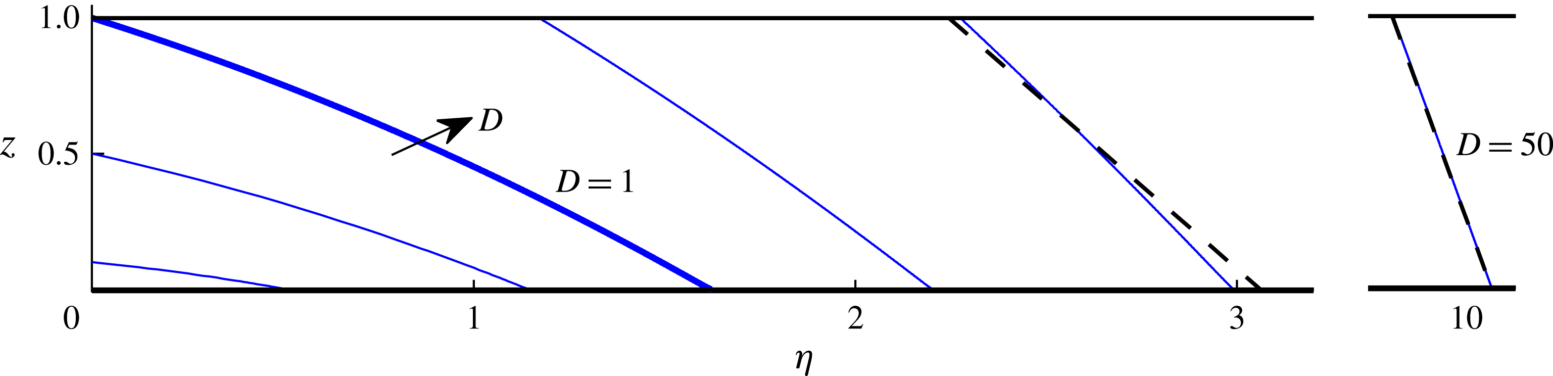
The long-term free-surface height
 $h({\it\eta})$
downstream of the outlet described by the similarity equations (3.14)–(3.16) for illustrative hydrostatic parameters
 $D=0.1,0.5,1,2,4$
and
 $50$
. The case
 $D=1$
(thick line) separates cases where the fluid contacts the upper boundary above the outlet (
 $D>1$
; regime
 $\text{C}$
) from those where the current remains detached below it (
 $D<1$
; regime
 $\text{B}$
). The analytical approximation obtained in appendix B is shown as a dashed black line for
 $D=4$
and 50.

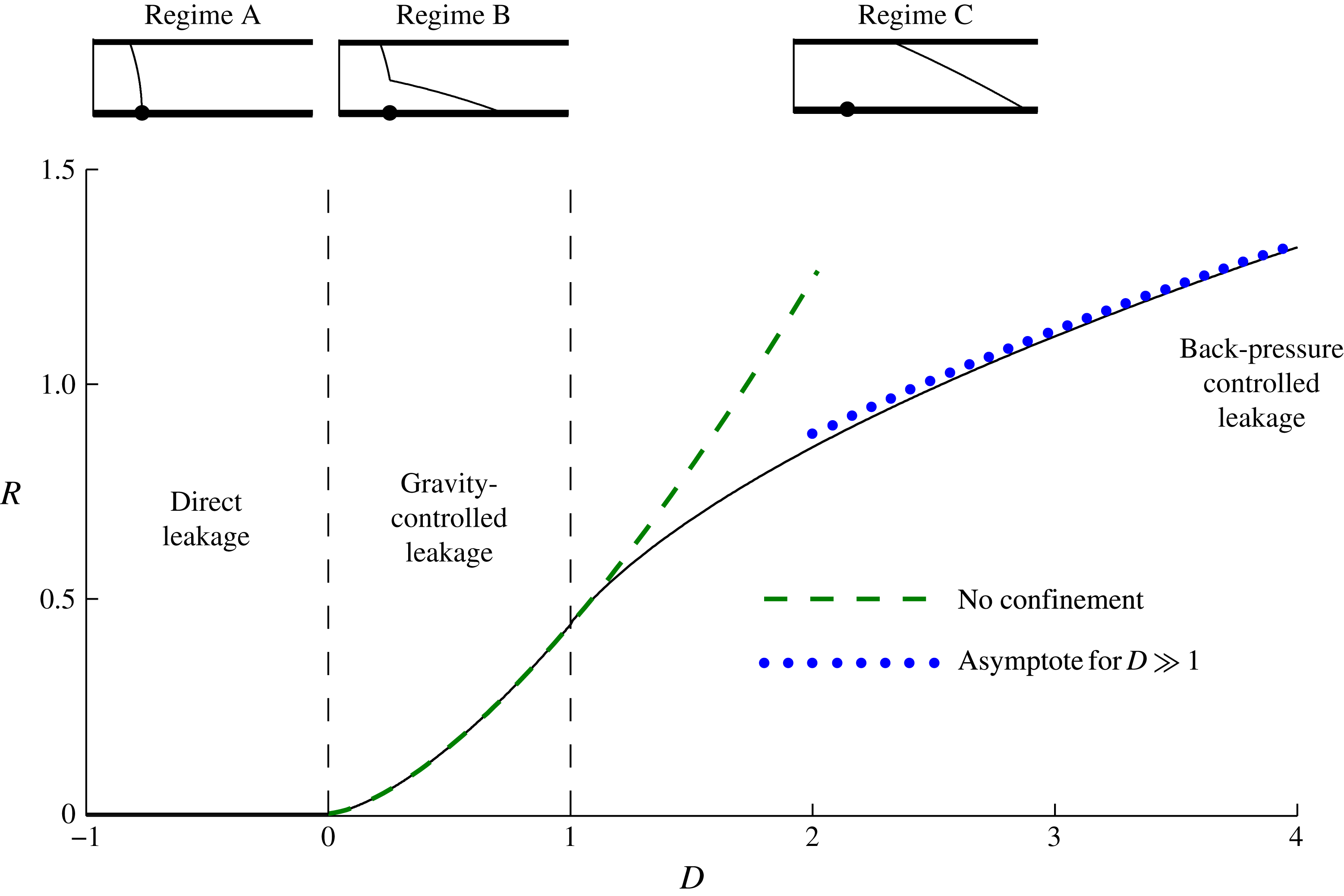
The retainment coefficient
 $R(D)$
in the long-term asymptotic evolution of the rate of change of the volume
 $\dot{V}\sim R\,t^{-1/2}$
as a function of
 $D$
. For
 $D\leqslant 0$
, all injected fluid leaks and
 $R=0$
(regime
 $\text{A}$
). For
 $0<D<1$
, the coefficient
 $R=0.443\,D^{3/2}$
given by (3.17c
) is shown as a dashed curve (green online, regime
 $\text{B}$
). For
 $D>1$
, the leakage rate is controlled by the back-pressure (regime
 $\text{C}$
). The switch in leakage dynamics from purely gravitational leakage for
 $0<D<1$
to fixed gravity-driven leakage with back-pressure for
 $D>1$
causes the curve of
 $R(D)$
to change from increasing superlinearly to sublinearly. This results in reduced fluid retainment compared to the same situation with the confining boundary absent. The asymptote for
 $D\gg 1$
given by (B 10) is shown as a dotted curve (blue online).

The relevant asymptotic conditions (3.5a,b
), which replace (3.10) for
 $D>1$
, are given by
 $$\begin{eqnarray}\displaystyle h(x_{U},t)=1,\quad q_{+}(t)=-\frac{\partial h}{\partial x}(x_{U},t)\sim \displaystyle \frac{\displaystyle D-1}{\displaystyle x_{U}(t)-X}\quad (t\rightarrow \infty ), & & \displaystyle\end{eqnarray}$$
where the latter follows on substitution of (3.18) into (3.5b
). Remarkably, a scaling analysis of (3.2)–(3.6) with (3.19a,b
) reveals the same similarity scalings (3.13) relevant if
 $0<D<1$
. This equivalence is coincidental: with
 $0<D<1$
, it arises from the diffusive scaling for the horizontal extent
 $x\sim t^{1/2}$
associated with a scaling of terms in (3.2) with
 $h\sim 1$
. The same scaling applies for
 $D>1$
because
 $x\sim t^{1/2}$
is also implied by the inverse dependence of
 $q_{+}\sim x/t$
on
 $x_{U}\sim x$
in (3.19b
), representing the reduction in the downstream flow rate arising from the build-up of back-pressure. In the analysis of Pegler et al. (Reference Pegler, Huppert and Neufeld2014b
), the relevant asymptotic scalings for
 $D>1$
instead imply that
 $q_{+}=O(1)$
and
 $x=O(t)$
, thus resulting in a different and more dramatic critical transition at
 $D=1$
than occurs here.
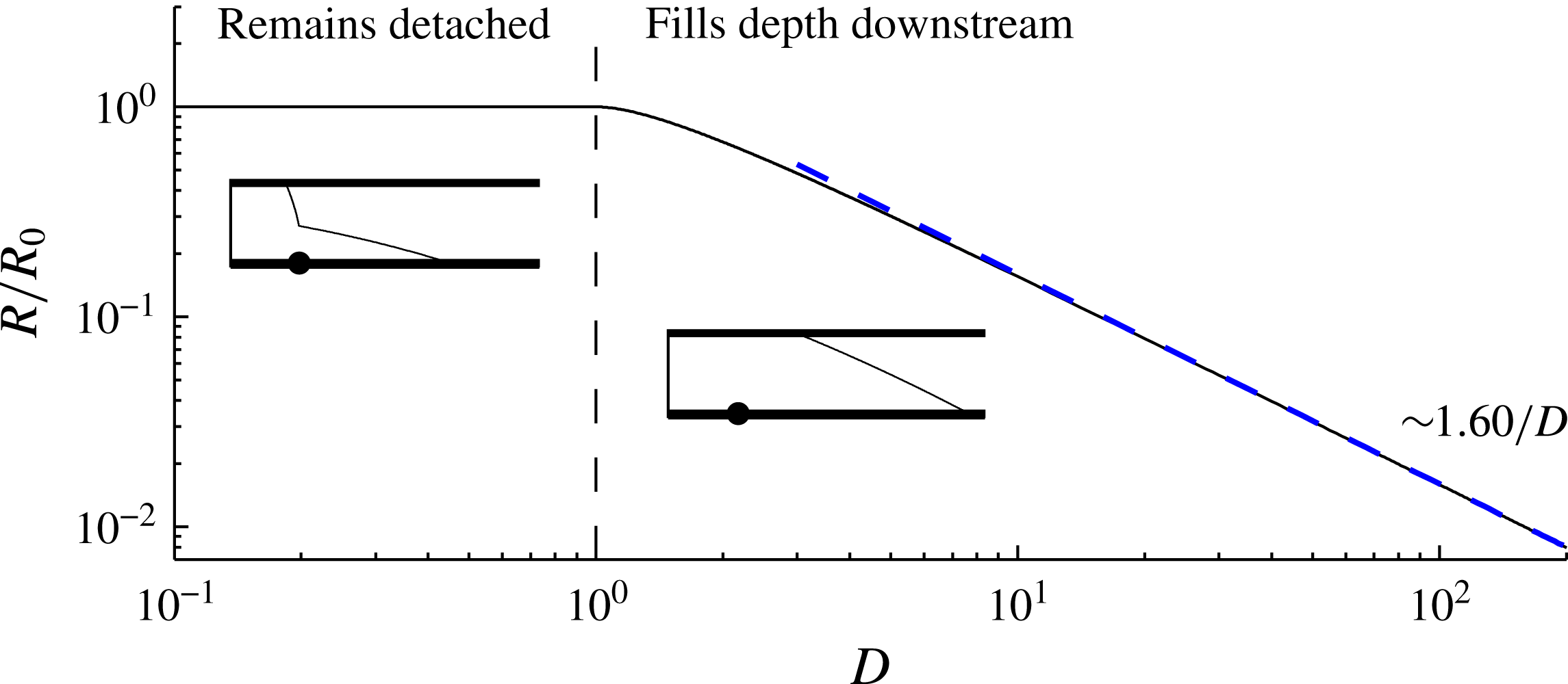
The asymptotic volume of fluid retained in the medium as a proportion of that which would be retained in the absence of the confining upper boundary C, as given by (3.21), measuring the relative reduction in fluid retainment by the confinement. The asymptote
 $C\sim 1.60/D$
for
 $D\gg 1$
is shown as a diagonal dashed line (blue online).

Recasting (3.19a,b ) in terms of (3.13), we obtain
 $$\begin{eqnarray}\displaystyle h({\it\eta}_{U})=1,\quad h^{\prime }({\it\eta}_{U})=-R=-\frac{D-1}{{\it\eta}_{U}}\quad \text{if }D>1. & & \displaystyle\end{eqnarray}$$
The system given by (3.14)–(3.16) and (3.20) was solved using a second-order finite difference scheme in which
 ${\it\eta}_{U}$
is treated as a shooting parameter. The height profiles for
 $D=2,4$
and 50 are plotted in figure 7 and the retainment coefficient is shown extended to cases of
 $D>1$
in figure 8. The free surface is seen to become shorter, steeper and lie further downstream as
 $D$
is increased. An analytical approximation obtained by considering the limit
 $D\gg 1$
is calculated in appendix B and plotted as a dashed black line for
 $D=4$
and 50. The associated asymptote for
 $R$
is shown as a dotted curve in figure 8.
The plot of the retainment coefficient
 $R$
in figure 8(b) shows that the function
 $R(D)$
switches from the superlinear relationship (3.17c
) for
 $0<D\leqslant 1$
to a sublinear relationship for
 $D>1$
. For values of
 $D>1$
,
 $R$
therefore drops below the long-term value applicable to an infinitely deep medium (shown extended into the region
 $D>1$
by the dashed curve (green online) in figure 8). The confinement therefore reduces the proportion of fluid retained to long times. To measure the increase in long-term fluid retainment relative to the leakage rate applicable without the confinement given by (3.17c
) and denoted here by
 $R_{0}=0.433D^{3/2}$
, we calculate the ratio
 $$\begin{eqnarray}C=\frac{R}{R_{0}}=\left\{\begin{array}{@{}ll@{}}1 & D\leqslant 1,\\ {\sim}\!1.60/D & D\rightarrow \infty ,\end{array}\right.\end{eqnarray}$$
which we have plotted in figure 9. The reduction of
 $C$
below unity for
 $D>1$
implies a reduction in fluid retainment compared to the same situation without the confinement. The large-
 $D$
asymptote in (3.21) is determined using the leading term in (B 10) and is shown as a blue diagonal dashed line in figure 9. The presence of the upper boundary is found to reduce the long-term proportion retained by 10 % if
 $D=1.4$
, by 50 % if
 $D=2.9$
and by 90 % if
 $D=16$
. The enhancement of vertical migration through a geological formation by confinement is therefore significant for large
 $D$
. This conclusion is in complete contrast to the effect of confinement found in situations where back-pressure is dominated by the viscous stresses associated with mobilizing ambient fluid (Pegler et al.
Reference Pegler, Huppert and Neufeld2014b
). In that situation, the approximate constancy of the back-pressure implies that the reduction of leakage caused by constraining the hydrostatic head remains a dominant effect to long times. In the present situation, the reduction of leakage caused by constraining the hydrostatic head is instead ultimately overridden by the long-term build-up of back-pressure and, moreover, results in greater long-term leakage than would occur if the confining boundary were absent.
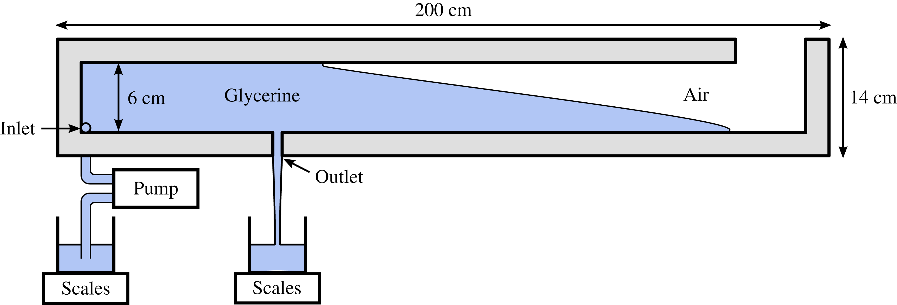
Schematic of our experimental Hele-Shaw cell.

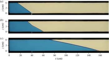
Sequence of photographs showing the evolution of experiment (d), as described in table 1: (a)
 $t=50$
s, (b)
 $t=100$
s, (c)
 $t=500$
s. The images have been stretched vertically by a factor of four. Our theoretically predicted position of the free surface is shown as a solid black curve. No fitting parameters have been used in making the comparison.

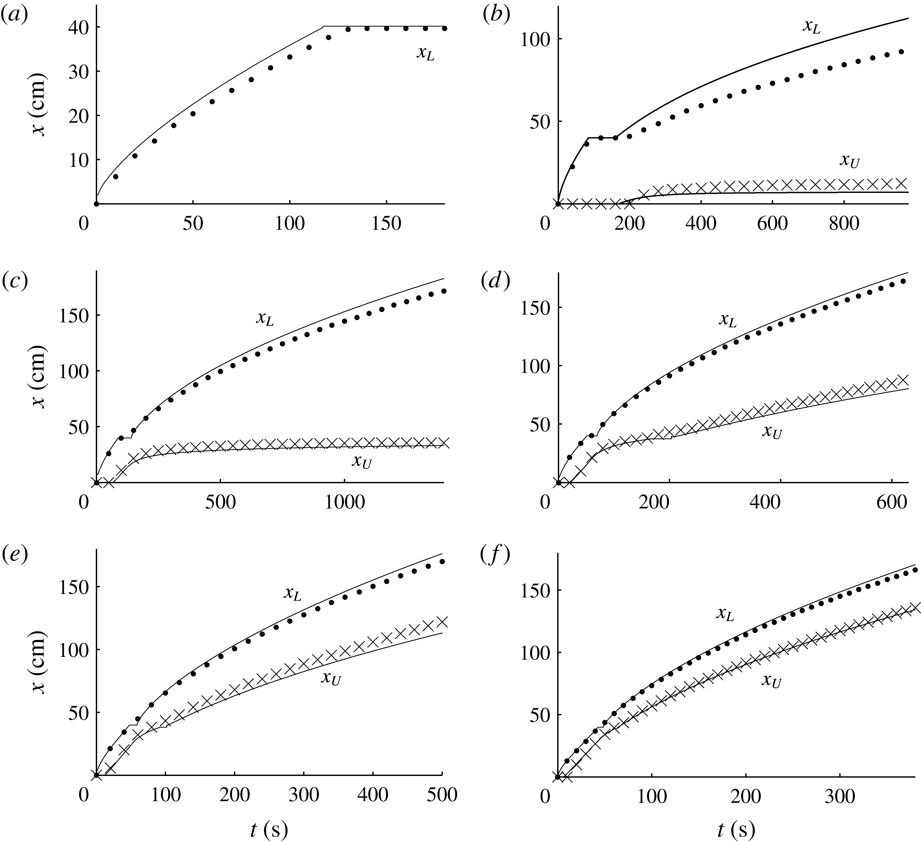
Comparisons between our experimental data for contact-line positions,
 $x_{L}(t)$
(filled circles) and
 $x_{U}(t)$
(crosses), and our theoretical predictions (solid curves), for the six experiments listed in table 1: (a)
 $D=-0.30$
; (b)
 $D=0.28$
; (c)
 $D=1.04$
; (d)
 $D=1.93$
; (e)
 $D=3.02$
; (f)
 $D=5.21$
.

4. Experimental study
We conducted a series of laboratory experiments to compare with our theoretical predictions. Our experiments were performed in a Hele-Shaw cell composed of two acrylic sheets, each 200 cm long and 14 cm high (see figure 10) and spacing
 $w\approx 0.38\pm 0.01~\text{cm}$
, forming a porous medium of permeability
 $k=w^{2}/12$
and porosity
 ${\it\phi}=1$
. The gap width was set by spacers, which bounded a confined region of internal height
 $H=6~\text{cm}$
. An opening of horizontal breadth
 $b=0.6~\text{cm}$
, vertical length
 $l=4~\text{cm}$
and central distance
 $x_{F}=40~\text{cm}$
from the left-hand edge was left in the lower spacer to form the outlet. The working fluid was glycerine of kinematic viscosity
 ${\it\nu}\equiv {\it\mu}/{\it\rho}\approx 4.35$
–
 $8.08\pm 0.02~\text{cm}^{2}~\text{s}^{-1}$
, which was measured before each experiment using a U-tube viscometer. Slight absorption of water from air caused the viscosity to vary between experiments.
The glycerine was injected into the medium through an inlet located at the lower left-hand corner of the cell using a peristaltic pump. The rate of injection
 $q_{0}$
was monitored by measuring the weight of the glycerine supply over the course of the experiment. The experiments were recorded using a digital camera and the recorded images analysed to obtain the positions of the upper and lower contact lines
 $x_{U}(t)$
and
 $x_{L}(t)$
. The value for the outlet permeability
 $k_{F}\approx 7.5\times 10^{-3}~\text{cm}^{2}$
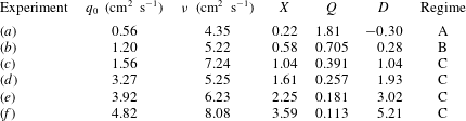
was determined empirically from calibration experiments in which the leakage rate was monitored over time. The parameters for six of our experiments (a)–(f), listed in table 1, spanned hydrostatic parameters from
 $D=-0.30$
to 5.21. Experiment (d) is shown in supplementary movie 1 available at http://dx.doi.org/10.1017/jfm.2015.315, and compared with our theoretically predicted interface position in the time-lapse sequence of figure 11. The measured frontal positions are compared with the theoretical predictions for all the experiments in figure 12. No fitting parameters have been used. Generally excellent agreement is seen between the data and the predictions.
Slight overprediction of the frontal positions
 $x_{L}(t)$
can be attributed to rounding of the noses of our experimental currents (see figure 11), which is not accommodated in our idealized theoretical model. We expect this rounding to be caused by a combination of the surface tension between glycerine and air and the traction exerted along the base of the current by the lower boundary. The discrepancy is most significant in experiment (b) because the region of the current downstream of the outlet is thinnest in that case and hence more sensitive to the effects of a rounded nose. Slight underprediction of the positions of the upper contact line
 $x_{U}(t)$
can likewise be attributed to the meniscus of the glycerine extending slightly along the top boundary.
Parameter values used in our experiments, arranged in order of ascending hydrostatic parameter
 $D$
.

5. Conclusions
We have considered the invasion of a dry porous medium by fluid in situations where the medium is confined vertically by horizontal boundaries, with one boundary containing a localized outlet or leakage point. It was found that, if the invading fluid can fill the full depth of the medium in the region of the leakage zone, then the long-term volume of fluid that leaks can be significantly greater than the rates of leakage obtained from previous studies of leakage in infinitely deep porous media. The enhancement of leakage arises from the build-up of back-pressure resulting from driving the invading fluid downstream of the leakage point. The rate of vertical fluid migration through the subsurface can therefore be much greater than predicted by studies which assume infinite depth, in situations where the rock forms layered strata, as is typical in sedimentary geological formations. Excellent agreement was obtained between the predictions and data from a new series of laboratory experiments.
Our primary theoretical results were to show that the long-term asymptotic flow can be classified into three distinct regimes by a dimensionless parameter
 $D$
. When positive,
 $D$
is the ratio of the steady-state height of the current at which the leakage driven by gravity alone balances the injection rate, to the depth of the medium. If
 $D<0$
, gravity acting along the outlet alone can independently drive a leakage rate which balances the injection rate. In those cases, all the invading fluid leaks directly through the outlet, with no fluid propagating downstream of it.
If
 $0<D<1$
, the injection rate is large enough to accumulate fluid above the outlet but small enough that the current remains detached from the upper boundary to long times. The hydrostatic head above the outlet approaches the asymptotic height at which gravity-driven leakage balances the injection rate, equivalent to the situation applicable to leakage from an infinitely deep porous medium. Likewise, the asymptotic proportion of injected fluid retained decreases according to
 $0.433D^{3/2}t^{-1/2}$
. The rate of leakage therefore balances the rate of injection asymptotically with a coefficient that increases superlinearly with the asymptotic hydrostatic head above the outlet
 $D$
.
If
 $D>1$
, there is a critical transition as the current fills the entire depth of the medium above the outlet and the free surface proceeds to migrate downstream indefinitely. Filling the full depth of the medium downstream of the outlet fixes gravity-driven leakage at a constant rate, but introduces a new force driving leakage given by the back-pressure associated with driving the invading fluid downstream of the outlet. Although the rate at which leakage is driven by gravity becomes constant as a result of fixing the hydrostatic head at the depth of the medium, the increase in back-pressure over time causes the leakage rate to approach the injection rate asymptotically. In this regime, the proportion of injected fluid retained approaches the asymptote
 $R(D)t^{-1/2}$
, where the function
 $R(D)$
is sublinear (with an asymptote
 $R(D)\sim (D/2)^{1/2}$
for
 $D\gg 1$
), contrasting with the superlinear relationship applicable for
 $0<D<1$
. The presence of the upper boundary therefore causes the rate at which fluid is retained in the medium to be potentially considerably smaller than if
 $D<1$
.
The conclusion relating to the effect of confinement on vertical migration is different to that which has been found in situations where an aquifer is saturated by an ambient viscous fluid (Pegler et al.
Reference Pegler, Huppert and Neufeld2014b
). In that situation, the back-pressure originates primarily from the displacement of ambient fluid towards the far field and hence there is relatively little change in back-pressure resulting from the introduction of invading fluid. The leakage rate is therefore effectively fixed once the depth of the medium above the outlet becomes filled, thus resulting in substantially more fluid retained to long times than occurs in the analogous cases where
 $D<1$
. This contrasts completely with the present situation, where the effect of constraining gravity-driven leakage from fixing the hydrostatic head at the depth of the medium is ultimately overridden by a significant build-up of pressure arising from the accumulation of injected fluid downstream of the leakage point. In summary, while the effect of confining boundaries can significantly reduce long-term leakage in aquifers saturated by an ambient fluid, the results of this paper indicate that confinement can only increase vertical migration if the host rock is unsaturated.
Acknowledgements
This work was supported by the PANACEA project funded by the European Commission. We are grateful to C. Hitch and D. Page-Croft for assistance in the preparation of our laboratory apparatus. The research of J.A.N. is supported by a Royal Society University Research Fellowship. H.E.H. is partially supported by a Wolfson Royal Society merit award and a Leverhulme Emeritus Fellowship.
Supplementary movie
Supplementary movie is available at http://dx.doi.org/10.1017/jfm.2015.315.
Appendix A. Frontal contact-line evolution
We derive the evolution equation for the layer fronts (2.8) from the frontal conditions (2.8a,b
). Differentiating (2.8a
) with respect to
 $t$
, rearranging for
 ${\dot{x}}_{L}$
and using (2.6a
) to substitute for
 $\partial h/\partial t$
in favour of the flux gradient
 $\partial q/\partial x$
, we obtain
 $$\begin{eqnarray}{\dot{x}}_{L}=-\frac{\partial h/\partial t}{\partial h/\partial x}=\frac{{\it\phi}^{-1}\partial q/\partial x}{\partial h/\partial x}=\lim _{x\rightarrow x_{L}}\left(\frac{q}{{\it\phi}h}\right)=\frac{u}{{\it\phi}},\end{eqnarray}$$
where all the quantities involving a partial derivative are evaluated a short distance upstream of
 $x=x_{L}$
. The third equality follows from l’Hôpital’s rule, which is applicable because the flux
 $q$
and the thickness
 $h$
both vanish together in the limit
 $x\rightarrow x_{L}$
in accord with (2.8a,b
).
Appendix B. Analytical approximation for
 $D\gg 1$

We determine an analytical approximation for the solution to the asymptotic similarity system given by (3.14), (3.15) and (3.20) for cases of
 $D\gg 1$
. With reference to (3.7), this corresponds to the physical limits of a shallow medium, a high rock permeability or a low outlet permeability, for example. It will be found to provide a reasonable approximation for
 $D\gtrsim 2$
.
The free surfaces in the numerical solutions with
 $D=4$
and 50 shown in figure 7 have a relatively short horizontal extent compared to the distance of the free surface from the outlet (
 ${\rm\Delta}{\it\eta}\equiv ({\it\eta}_{L}-{\it\eta}_{U})\ll {\it\eta}_{U}$
). This motivates an analysis based on a small perturbation to the horizontal coordinate,
 $$\begin{eqnarray}{\it\eta}={\it\eta}_{0}+\tilde{{\it\eta}},\end{eqnarray}$$
where
 ${\it\eta}_{0}$
is a constant representing the leading-order horizontal position of the interface, to be determined, and
 $\tilde{{\it\eta}}\ll {\it\eta}_{0}$
is the perturbation to the spatial coordinate. Substituting (B 1) into (3.14) and neglecting higher-order terms, we obtain
 $$\begin{eqnarray}-\!{\textstyle \frac{1}{2}}{\it\eta}_{0}h^{\prime }\approx (hh^{\prime })^{\prime },\end{eqnarray}$$
where
 $h=h(\tilde{{\it\eta}})$
and we have used a prime here to denote
 $\text{d}/\text{d}\tilde{{\it\eta}}$
. With
 $\tilde{{\it\eta}}_{U}={\it\eta}_{U}-{\it\eta}_{0}$
and
 $\tilde{{\it\eta}}_{L}={\it\eta}_{L}-{\it\eta}_{0}$
, the conditions at the upper boundary (3.20a,b
) and front of the current (3.15a,b
) take the leading-order forms
 $$\begin{eqnarray}\displaystyle h(\tilde{{\it\eta}}_{U})=1,\quad h^{\prime }(\tilde{{\it\eta}}_{U})\approx -(D-1)/{\it\eta}_{0}, & & \displaystyle\end{eqnarray}$$
 $$\begin{eqnarray}\displaystyle h(\tilde{{\it\eta}}_{L})=0,\quad h^{\prime }(\tilde{{\it\eta}}_{L})\approx -{\textstyle \frac{1}{2}}{\it\eta}_{0}. & & \displaystyle\end{eqnarray}$$
Integrating (B 2) subject to (B 3b ) and (B 4b ), we obtain
 $$\begin{eqnarray}\displaystyle h^{\prime }=-{\textstyle \frac{1}{2}}{\it\eta}_{0}\quad \text{where }{\it\eta}_{0}=[2(D-1)]^{1/2}. & & \displaystyle\end{eqnarray}$$
Equation (B 5a
) shows that the free surface is linear to leading order, with a slope
 $h^{\prime }$
that is steeper for solutions of larger extent
 ${\it\eta}_{0}$
. This is consistent with the flow rate
 $u$
in the free-surface region being proportional to the slope in accord with (2.5). Integration of (B 5a
) subject to (B 3a
) and (B 4a
) yields
 $$\begin{eqnarray}\displaystyle h(\tilde{{\it\eta}})=\frac{\tilde{{\it\eta}}_{L}-\tilde{{\it\eta}}}{{\rm\Delta}{\it\eta}},\quad \text{where }{\rm\Delta}{\it\eta}\equiv ({\it\eta}_{L}-{\it\eta}_{U})=\frac{2}{{\it\eta}_{0}}=\left[\frac{2}{D-1}\right]^{1/2}. & & \displaystyle\end{eqnarray}$$
To determine the edges of the free surface
 $\tilde{{\it\eta}}_{U}$
and
 $\tilde{{\it\eta}}_{L}$
, we utilize the equation of global volume conservation, which is given dimensionally by
 $$\begin{eqnarray}\int _{0}^{t}q_{+}({\it\tau})\,\text{d}{\it\tau}={\it\phi}\int _{x_{F}}^{x_{L}(t)}h(x,t)\,\text{d}x.\end{eqnarray}$$
This equation relates the time-integrated volumetric flux of input downstream
 $q_{+}(t)$
to the total volume of fluid in that region. Recasting (B 7) in terms of the similarity variables (3.13), evaluating the time integral on the left-hand side and using (3.20b
) and (B 6a
), we obtain
 $$\begin{eqnarray}\displaystyle 2R=\frac{2(D-1)}{{\it\eta}_{U}}=\int _{0}^{{\it\eta}_{L}}h\,\text{d}{\it\eta}\approx {\it\eta}_{U}+\frac{{\rm\Delta}{\it\eta}}{2}, & & \displaystyle\end{eqnarray}$$
where the first term in the last equation originates from the volume between the outlet and the upper contact line
 $0<{\it\eta}<{\it\eta}_{U}$
and the second term from the free-surface region
 ${\it\eta}_{U}<{\it\eta}<{\it\eta}_{L}$
. Substituting
 ${\it\eta}_{U}={\it\eta}_{0}-\tilde{{\it\eta}}_{U}$
and neglecting higher-order terms in
 $\tilde{{\it\eta}}\ll {\it\eta}_{0}$
, we obtain the first-order perturbations to the contact-line positions
 $$\begin{eqnarray}\displaystyle \tilde{{\it\eta}}_{U}=-{\textstyle \frac{1}{4}}{\rm\Delta}{\it\eta},\quad \tilde{{\it\eta}}_{L}={\textstyle \frac{3}{4}}{\rm\Delta}{\it\eta}. & & \displaystyle\end{eqnarray}$$
The asymptotic solution given by (B 6a,b
) and (B 9a,b
) is shown as a black dashed line for the examples of
 $D=4$
and 50 in figure 7, showing good agreement with our numerical solution.
Using (B 5), (B 6b
) and (B 9a
) to evaluate
 ${\it\eta}_{U}={\it\eta}_{0}+\tilde{{\it\eta}}_{U}$
in the first equation in (B 8) and neglecting the higher-order terms, we obtain the leading-order coefficient
 $R$
, along with its first-order correction, as
 $$\begin{eqnarray}R\sim \left(\frac{D-1}{2}\right)^{1/2}\left[1+\frac{1}{4(D-1)}\right]\quad (D\gg 1),\end{eqnarray}$$
which is plotted as a dotted curve (blue online) in figure 8.