


1 Introduction
The swept-wing geometry gives rise to a three-dimensional laminar boundary layer, featuring the so-called cross-flow (CF). Cross-flow is a weak secondary flow component, perpendicular to the outer inviscid streamline, caused by the relative imbalance between the pressure and inertial forces within the boundary layer. The CF component inherently forms an inflection point, which results in the inviscid cross-flow instability (CFI). This instability is characterised by co-rotating vortices of stationary (steady) or travelling (unsteady) nature, depending on external disturbances (Downs & White Reference Downs and White2013). An extensive review on the topic has been compiled by Saric, Reed & White (Reference Saric, Reed and White2003).
Cross-flow instability has a pivotal role in the process of laminar-to-turbulent transition. As such, suppression of CFI presents a promising route towards transition delay and aerodynamic drag reduction (Joslin Reference Joslin1998). Different strategies have been proposed and investigated to control transition induced by stationary CFI modes. A brief review of these can be found in Serpieri, Yadala Venkata & Kotsonis (Reference Serpieri, Yadala Venkata and Kotsonis2017). A strategy that has received considerable attention is the use of discrete roughness elements (DRE), first proposed by Saric and co-workers (see Saric et al. (Reference Saric, Reed and White2003)) and later generalised as upstream flow deformation (UFD) by Wassermann & Kloker (Reference Wassermann and Kloker2002). Primary stationary CFI modes appear in a selected band of unstable (or critical) spanwise wavenumbers and eventually undergo secondary instability leading to final transition (Saeed, Mughal & Morrison Reference Saeed, Mughal and Morrison2016). The DRE/UFD strategy is based on forcing shorter wavelength CFI modes (i.e. subcritical modes), which deter the growth of the critical mode, thus delaying transition. While initial wind-tunnel tests (Saric et al. Reference Saric, Reed and White2003; Schuele, Corke & Matlis Reference Schuele, Corke and Matlis2013) and numerical simulations (Wassermann & Kloker Reference Wassermann and Kloker2002) have shown successful transition delay, later flight tests (Saric et al. Reference Saric, West, Tufts and Reed2015) were inconclusive. Additionally, a recent study by Lovig, Downs & White (Reference Lovig, Downs and White2014) indicated a dependency of the DRE performance on background roughness and baseline transition location. The aforementioned studies indicate a high sensitivity of the DRE/UFD technique to flow conditions, and particularly background disturbance levels (private communication with W. Saric).
An alternative CFI control strategy is based upon direct suppression of the inherent cause of the instability, which in this case is the CF component of the boundary layer. Numerical simulations employing wall suction (Messing & Kloker Reference Messing and Kloker2010) or body forcing (Dörr & Kloker Reference Dörr and Kloker2015b ), configured such as to suppress the CF component, were proven to delay transition. Dörr & Kloker achieved base-flow modification by applying a body force against the local CF. They observed a reduction in the amplification rates of both the steady and unsteady CFI modes, thus stabilising the boundary layer and yielding transition delay. An essential difference from the DRE/UFD approach is that base-flow modification relies directly on the suppression of the mean boundary layer, rendering its performance relatively independent of the nature of CFI (i.e. modes’ wavelength and stationary or travelling type). However, to this point, the concept of base-flow modification for suppression of CFI has not been demonstrated experimentally.
In the present study, the base-flow modification strategy is demonstrated experimentally, by alternating current dielectric barrier discharge (AC-DBD) plasma actuators. Thorough reviews on plasma actuators and their applications can be found in Corke, Enloe & Wilkinson (Reference Corke, Enloe and Wilkinson2010), Wang et al. (Reference Wang, Choi, Feng, Jukes and Whalley2013) and Benard & Moreau (Reference Benard and Moreau2014). While the application of AC-DBD actuators on two-dimensional boundary layers has been extensively studied, utilisation of these devices to control CFI is rather limited (e.g. Schuele et al. (Reference Schuele, Corke and Matlis2013), Dörr & Kloker (Reference Dörr and Kloker2015b ), Shahriari (Reference Shahriari2016), Serpieri et al. (Reference Serpieri, Yadala Venkata and Kotsonis2017), Wang, Wang & Fu (Reference Wang, Wang and Fu2017)). Prior to the experimental investigation, a preliminary theoretical/numerical study is performed. The stability of the boundary layer, under the influence of the plasma body force, is numerically estimated using the simple model proposed by Serpieri et al. (Reference Serpieri, Yadala Venkata and Kotsonis2017). Following the predictions of the model, experimental demonstration of the plasma-based base-flow modification is achieved by installing an AC-DBD plasma actuator that produces a two-dimensional body force, close to the leading edge of a swept-wing model. Two forcing conditions are investigated, namely forcing along and against the local CF. Infrared (IR) thermography is employed to visualise laminar-to-turbulent transition.
2 Methodology
2.1 Experimental set-up and measurement technique
The experiments were carried out in the closed-loop, Low Turbulence Tunnel (LTT) at TU Delft Aerodynamics (turbulence intensity
 ${<}0.15\,\%$
). The swept-wing model features an in-house designed airfoil shape (66018M3J), streamwise chord (c) of 1.27 m and a
 $45^{\circ }$
sweep. Details of the employed swept-wing model and the wind tunnel are given in Serpieri & Kotsonis (Reference Serpieri and Kotsonis2016) and Serpieri et al. (Reference Serpieri, Yadala Venkata and Kotsonis2017). The flow over the wing’s pressure side was investigated. For this study, the wing incidence angle was set at
 $\unicode[STIX]{x1D6FC}=3^{\circ }$
. Experiments were performed for three free-stream velocities, namely
 $U_{\infty }=25$
, 27.5 and
 $30~\text{m}~\text{s}^{-1}$
, corresponding to chord Reynolds numbers of 2.1, 2.3 and 2.5 million, respectively. The swept-wing reference system is referred to as
 $xyz$
. It is such that its
 $x$
axis is perpendicular to the leading edge,
 $y$
axis is perpendicular to the chord plane and
 $z$
axis is parallel to the leading edge. The corresponding velocity components are represented by
 $uvw$
. The free-stream velocity is referred to as
 $U_{\infty }$
.
IR thermography was employed to inspect the laminar-to-turbulent transition front (Saric, Carpenter & Reed Reference Saric, Carpenter and Reed2011; Serpieri et al.
Reference Serpieri, Yadala Venkata and Kotsonis2017). To enhance contrast, the swept-wing model was irradiated with six 1 kW halogen lamps, through glass windows in the test section. Surface temperature distributions were captured using an Optris PI640 IR camera with a thermal sensitivity of 75 mK, operating in the spectral band of
 $7.5{-}13~\unicode[STIX]{x03BC}\text{m}$
. Dewarping, deskewing and spatial calibration was applied in order to cast the raw images in the
 $xz$
plane. After the temperature of the wing surface has reached an equilibrium, the camera registers 100 snapshots, at a rate of 5 Hz for every tested flow case. These are averaged in order to increase the signal-to-noise ratio. It should be noted that the results presented here are used to extract pertinent features of the flow topology, such as transition location. As such, no effort was made to correct the measured temperatures for emissivity and reflectivity effects.
In this study, stationary CFI modes were forced at a spanwise wavelength of
 $\unicode[STIX]{x1D706}_{z}=8~\text{mm}$
which, for the tested flow conditions, is near the most unstable stationary mode as predicted by linear stability theory (LST). The choice for artificially forcing the critical CFI mode stems from a range of objectives. Most importantly, promotion of the critical mode presents a ‘worst case scenario’ for any given control scheme, thus ultimately giving a maximum bound on the performance of the control. Furthermore, for the studied flow conditions, natural (unforced) transition is downstream of the pressure minimum (located at
 $x/c\approx 0.63$
, see Serpieri et al. (Reference Serpieri, Yadala Venkata and Kotsonis2017)) and is dominated by laminar separation. DRE forcing further assists in bringing transition upstream and achieving CFI-dominated conditions. Finally, by conditioning the initial amplitude of individual CF vortices, a more uniform and spanwise invariant transition front is achieved. An array of micron-sized DREs with diameter
 $d_{DRE}=2~\text{mm}$
and height
 $k_{DRE}=60~\unicode[STIX]{x03BC}\text{m}$
was employed to lock the critical CFI mode (Saric et al.
Reference Saric, Reed and White2003). The DREs were installed near the wing leading edge, at
 $x/c=0.017$
(neutral point of
 $\unicode[STIX]{x1D706}_{z,crit}=8$
mm mode is at
 $x/c=0.0068$
). The ratio of DRE height and local displacement thickness is
 $k_{DRE}/\unicode[STIX]{x1D6FF}^{\ast }=0.47$
.
2.2 AC-DBD plasma actuator
In the vicinity of the leading edge attachment line of a swept-wing, inviscid streamlines are almost aligned with the
 $z$
direction. As such, forcing in the
 $x$
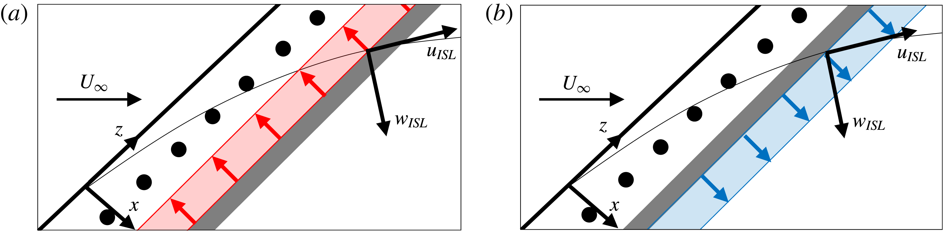
direction will largely impact the CF component of the base flow. This is capitalised upon in the present study, where an AC-DBD plasma actuator that generates a spanwise invariant plasma forcing was designed. This design is adopted to avoid unwanted forcing of CFI modes as well as to ensure a simple and robust forcing configuration (figure 1).
Schematic of the forcing mechanism (not to scale). Inviscid streamline (thin black line) and local velocity components (
 $u_{ISL},w_{ISL}$
). DRE arrangement (●) and plasma actuator exposed electrode (grey bar). (a)
 $-F_{x}$
plasma forcing (red arrows); (b)
 $F_{x}$
plasma forcing (blue arrows).
Due to the extreme sensitivity of CFI to surface roughness (Saric et al.
Reference Saric, Reed and White2003), it was imperative to ensure minimum protuberance due to the actuator. With this goal in mind, computer-controlled spraying of micrometric conductive silver particles was employed to fabricate the electrodes, with thicknesses in the order of a few microns.
 $500~\unicode[STIX]{x03BC}\text{m}$
thick polyethylene terephthalate (PET) foils were used as dielectric material. The foils were wrapped around the leading edge and extended to
 $x/c=0.69$
to form an uninterrupted smooth surface. The electrode width was
 $w=5~\text{mm}$
, on both sides of the dielectric, with no relative overlap or gap. Furthermore, AC-DBD actuators are known to impart unsteady fluctuations at the AC driving frequency, which can potentially trigger transition (Benard, Noté & Moreau Reference Benard, Noté and Moreau2017). This was observed in the study of Serpieri et al. (Reference Serpieri, Yadala Venkata and Kotsonis2017), which recommended forcing at higher frequencies (also discussed by Dörr & Kloker (Reference Dörr and Kloker2016)). Based on the above, forcing at
 $f_{ac}=10~\text{kHz}$
was employed for the present study. The actuator was installed such that the electrodes’ interface was at
 $x/c=0.035$
. Two plasma actuators were fabricated, one to exert
 $-F_{x}$
forcing (figure 1
a) and the second to exert
 $F_{x}$
forcing (figure 1
b) on the boundary layer. The air-exposed electrode was supplied with a sinusoidal AC signal of peak-to-peak amplitude between 5 and 9 kV, while the encapsulated electrode was grounded. The actuator was powered using a GBS Electronik Minipuls 4 high-voltage amplifier, controlled by LabView software.
It should be noted that the relative chordwise position of the DREs to the plasma actuator is not significant as long as they are positioned downstream of the first neutral point (to ensure the CFI is formed and growing). However, the position of the plasma actuator will affect its orientation with respect to the external streamline. Aligning the plasma body force to operate normal to the inviscid streamline is expected to enhance the effectiveness of the control, as this technique is based on attenuating the CF component.
2.3 Simplified plasma forcing model
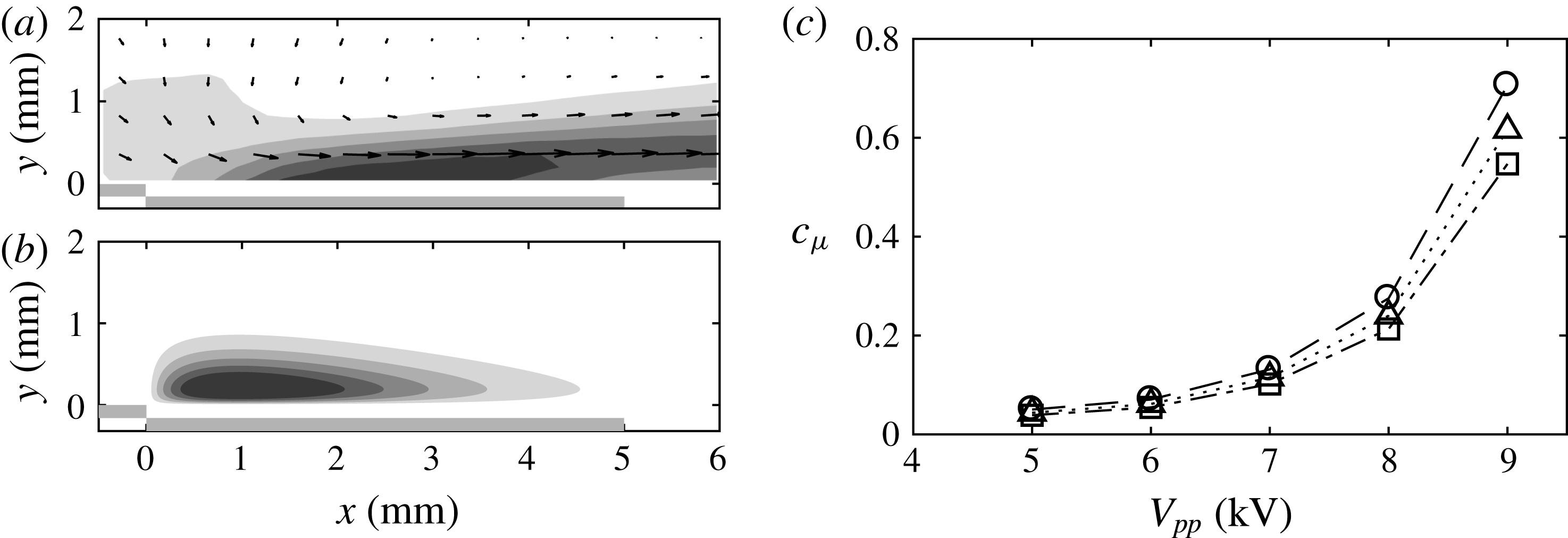
A number of parameters related to the flow and the AC-DBD actuator have an impact on boundary layer stability, which necessitates the definition of an efficient numerical model to carry out a preliminary assessment of the control effectiveness. With this objective, Serpieri et al. (Reference Serpieri, Yadala Venkata and Kotsonis2017) proposed a simplified model to demonstrate the effect of steady plasma forcing on boundary layer stability. This model is employed in the current study. An experimentally acquired, steady plasma body force (figure 2
b) was included into the boundary layer solver as a source term (
 $F_{x}/\unicode[STIX]{x1D70C}$
) in the
 $x$
-momentum equation. The steady two-dimensional incompressible boundary layer equations are solved to obtain the laminar boundary layer solution. This modified boundary layer yields the base-flow input for the linear stability solver, thus retrieving growth rates and
 $N$
factors of the amplified CFI modes.
3 Results
3.1 AC-DBD plasma actuator characterisation
The time-averaged velocity field induced by the actuator used in the current study, when operated at
 $V_{pp}=9~\text{kV}$
,
 $f_{ac}=10~\text{kHz}$
is shown in figure 2(a). This field was acquired in a dedicated characterisation experiment using high-speed particle image velocimetry (PIV), in quiescent conditions (Serpieri et al.
Reference Serpieri, Yadala Venkata and Kotsonis2017). The corresponding body force (figure 2
b) is computed using the empirical model proposed and validated by Maden et al. (Reference Maden, Maduta, Kriegseis, Jakirli, Schwarz, Grundmann and Tropea2013). The body-force magnitude was calibrated such that the integrated body-force value matches the thrust calculated from the experimental velocity field using the momentum balance method (Kotsonis et al.
Reference Kotsonis, Ghaemi, Veldhuis and Scarano2011). The effect of two-dimensional forcing on the stability of the boundary layer was investigated by introducing this steady, volume-distributed plasma body force
 $F_{x}(x,y),F_{y}=0$
(see Maden et al. (Reference Maden, Maduta, Kriegseis, Jakirli, Schwarz, Grundmann and Tropea2013), Dörr & Kloker (Reference Dörr and Kloker2015a
)), into the boundary layer solver.
(a) Time-averaged induced velocity-magnitude field for
 $V_{pp}=9~\text{kV}$
,
 $f_{ac}=10~\text{kHz}$
(six levels from 0 (white) to
 $3~\text{m}~\text{s}^{-1}$
(black)). The two grey lines below
 $y=0$
depict the electrodes of the AC-DBD plasma actuator. (b) Body force computed using the empirical model by Maden et al. (Reference Maden, Maduta, Kriegseis, Jakirli, Schwarz, Grundmann and Tropea2013) (six levels from 0 (white) to
 $3~\text{kN}~\text{m}^{-3}$
(black)). (c) Variation of momentum coefficient
 $c_{\unicode[STIX]{x1D707}}$
with input peak-to-peak voltage
 $V_{pp}$
(○:
 $U_{\infty }=25~\text{m}~\text{s}^{-1}$
, ▵:
 $U_{\infty }=27.5~\text{m}~\text{s}^{-1}$
, ▫:
 $U_{\infty }=30~\text{m}~\text{s}^{-1}$
).
The integrated actuator thrust (
 $T_{x}$
) is further used to compute the momentum coefficient
 $c_{\unicode[STIX]{x1D707}}$
by (3.1),
 $$\begin{eqnarray}c_{\unicode[STIX]{x1D707}}=\frac{T_{x}}{\frac{1}{2}\unicode[STIX]{x1D70C}u_{e}^{2}\unicode[STIX]{x1D703}_{u}},\end{eqnarray}$$
where
 $u_{e}$
is the local (at electrode interface) boundary layer edge velocity and
 $\unicode[STIX]{x1D703}_{u}$
is the local momentum thickness of the corresponding baseline case along the chordwise direction. The momentum coefficient
 $c_{\unicode[STIX]{x1D707}}$
is used to compare the actuator’s authority for different flow conditions. The variation of
 $c_{\unicode[STIX]{x1D707}}$
with the input voltage for different free-stream velocities investigated in the current study is presented in figure 2(c). Henceforth,
 $c_{\unicode[STIX]{x1D707}}$
will be employed to discuss the different forcing conditions.
3.2 Base-flow and stability modification
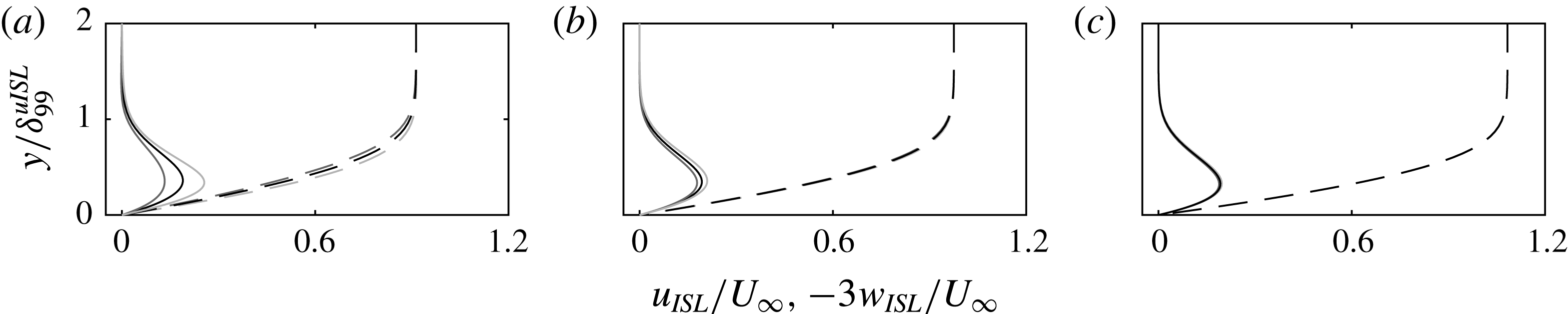
The numerical boundary layer solutions at three different chord locations for the baseline (i.e. no forcing),
 $-F_{x}$
and
 $F_{x}$
forcing cases are shown in figure 3. At the actuator’s location, the external inviscid streamline angle is approximately
 $55^{\circ }$
with respect to
 $x$
. Thus,
 $F_{x}$
forcing imparts momentum partially along the cross-flow and has an enhancing effect on both the streamwise and spanwise velocity components. Contrary to this,
 $-F_{x}$
forcing opposes both velocity components, thus diminishing their magnitude, as evident in figure 3. However, the profiles of the forced cases tend to collapse on the baseline flow case close to
 $x/c\approx 0.3$
(figure 3
c). This is expected considering the low magnitude of the body force and its localised spatial extent, as shown in figure 2.
Computed boundary layer velocity profiles for
 $Re_{c}=2.1\times 10^{6}$
(
 $U_{\infty }=25~\text{m}~\text{s}^{-1}$
), parallel (
 $u_{ISL}$
: dashed line) and perpendicular (
 $w_{ISL}$
: solid line, magnified by factor of three) to the local inviscid streamline at three chord locations, namely: (a)
 $x/c=0.05$
, (b)
 $x/c=0.1$
and (c)
 $x/c=0.3$
. The three cases shown are: baseline (black),
 $c_{\unicode[STIX]{x1D707}}=-0.71$
(dark grey),
 $c_{\unicode[STIX]{x1D707}}=0.71$
(light grey). The wall normal axis is non-dimensionalised with the boundary layer thickness based on
 $0.99\cdot u_{ISL}$
from the local unforced profile.
Stability diagrams for stationary CFI modes (i.e. zero frequency), indicating growth rates (
 $\unicode[STIX]{x1D6FC}_{i}$
) and
 $N$
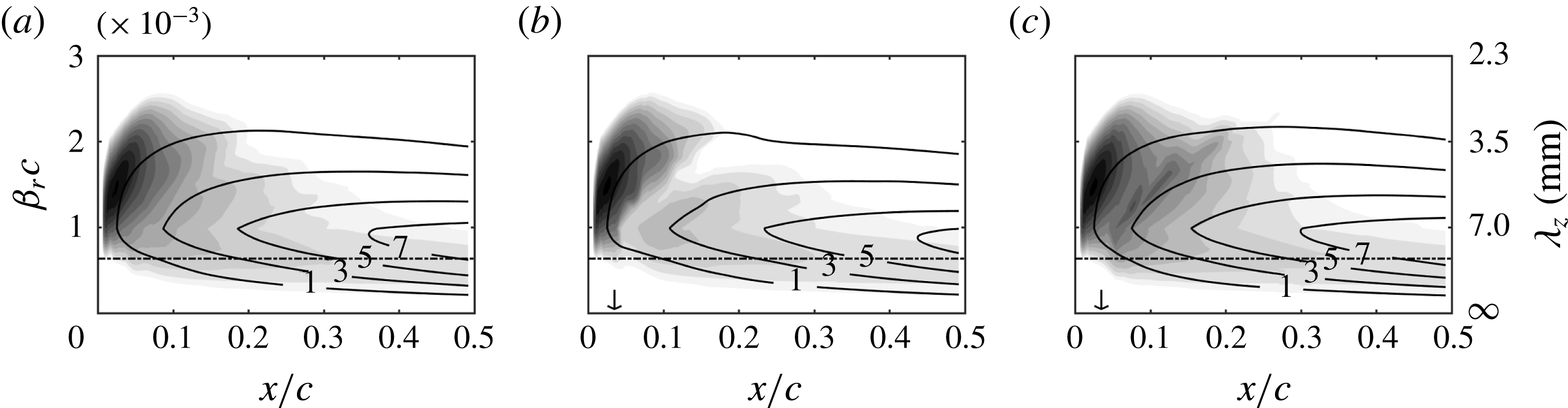
factors, for the three tested cases shown in figure 3, are presented in figure 4. It is evident that the
 $\unicode[STIX]{x1D706}_{z,crit}=8~\text{mm}$
mode (chosen as the mode forced by DRE in the experiment, indicated by the dashed line) is one of the most unstable stationary modes for these conditions. Comparing the stability plots of the baseline (figure 4
a) and forced cases (figures 4
b and c) confirms that
 $-F_{x}$
forcing hinders the growth of stationary CFI modes, thus stabilising the boundary layer. As expected,
 $F_{x}$
forcing augments the growth rate of all stationary CFI modes and has a destabilising effect on the boundary layer. In both cases, the effect of forcing is rather local. Indeed, upstream of
 $x/c\approx 0.3$
, the growth rates show insignificant disparity, as suggested by the almost identical velocity profiles at that station (figure 3
c). However, the integral effect on the stability of the boundary layer, illustrated by the
 $N$
factor, is evident well downstream of the forcing location. Assuming that the critical
 $N$
factor does not significantly change due to actuation, the transition location can be expected to shift downstream with
 $-F_{x}$
forcing and upstream with
 $F_{x}$
forcing.
Streamwise amplification rate (
 $-\unicode[STIX]{x1D6FC}_{i}c$
) (15 levels from 0 (white) to 65 (black)) (spanwise wavenumber
 $\unicode[STIX]{x1D6FD}_{r}=2\unicode[STIX]{x03C0}/\unicode[STIX]{x1D706}_{z}$
). Black contour lines show the amplification factor (
 $N$
). Dash-dotted black line indicates the
 $\unicode[STIX]{x1D706}_{z,crit}=8~\text{mm}$
mode. The three cases shown are: (a) baseline, (b)
 $c_{\unicode[STIX]{x1D707}}=-0.71$
, (c)
 $c_{\unicode[STIX]{x1D707}}=0.71$
. Vertical arrows in (b) and (c) represent the location of the plasma forcing.
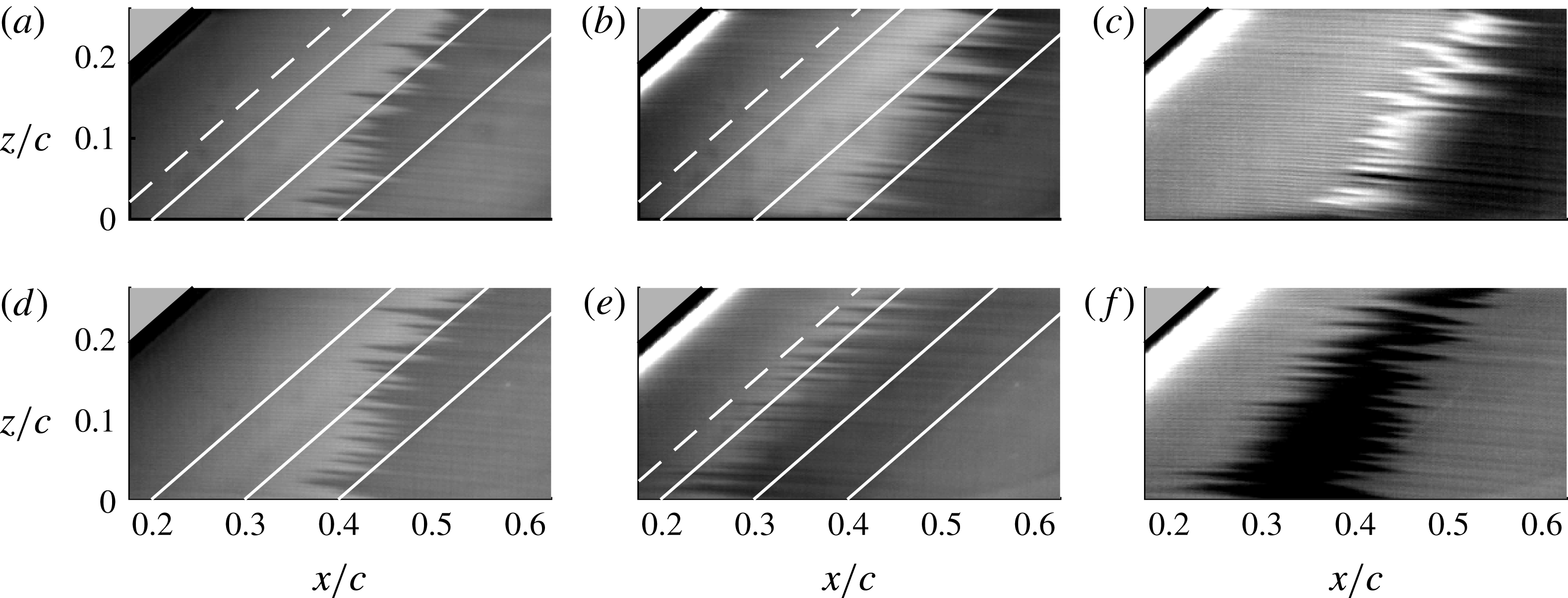
IR thermography mean fields (
 $Re_{c}=2.1\times 10^{6}$
,
 $U_{\infty }=25~\text{m}~\text{s}^{-1}$
). The flow comes from the left. The IR mean fields are dewarped and plotted in the
 $xz$
plane. (a) Baseline. (b)
 $-F_{x}$
(
 $c_{\unicode[STIX]{x1D707}}=-0.71$
). (c) Subtraction of (a) from (b). (d) Baseline. (e)
 $F_{x}$
(
 $c_{\unicode[STIX]{x1D707}}=0.71$
). (f) Subtraction of (d) from (e). The solid white lines represent constant chord positions. Dashed line at
 $x/c=0.15$
refers to figure 6(a).
3.3 Thermal imaging of the flow topology
The flow topology, visualised through IR imaging, is shown in figure 5 for
 $Re_{c}=2.1\times 10^{6}$
(
 $U_{\infty }=25~\text{m}~\text{s}^{-1}$
). In the baseline (i.e. no forcing) cases shown in figures 5(a) and (d) the actuators configured for
 $-F_{x}$
and
 $F_{x}$
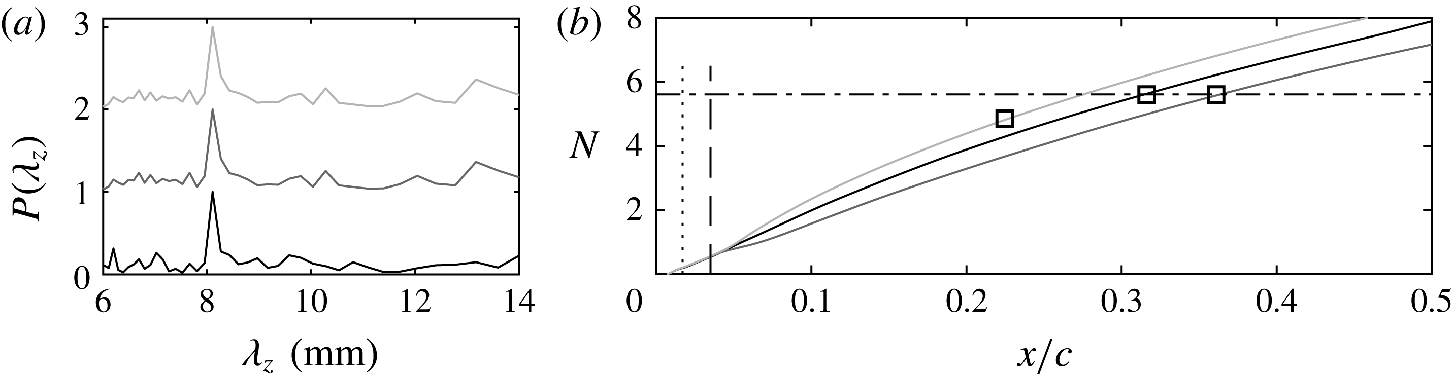
forcing, respectively, are installed on the wing; however, they are not operative. The observed flow arrangement is the result of the steady forcing by the installed DRE. Spatial fast Fourier transform (FFT) analysis along constant chord lines shown in figure 6(a) confirms that the
 $\unicode[STIX]{x1D706}_{z,crit}=8~\text{mm}$
mode forced by the DRE is indeed the spanwise dominant mode in the boundary layer. It should be stressed that no thermal calibration was performed on the recorded IR images. As such, the FFT analysis is only used to identify the spectral components and not the amplitude of CFI modes. To this effect, the wavenumber spectra presented in figure 6(a) are normalised with their respective maxima. Furthermore, in both baseline IR fields, the laminar breakdown occurs along the characteristic jagged pattern reported for CFI-induced transition (Saric et al.
Reference Saric, Reed and White2003, Reference Saric, Carpenter and Reed2011; Serpieri & Kotsonis Reference Serpieri and Kotsonis2016), at approximately the same chordwise position (
 $x/c\approx 0.32$
).
The flow arrangement when
 $-F_{x}$
and
 $F_{x}$
plasma forcing is applied is shown in figures 5(b) and (e) respectively. FFT analysis again confirms that the spanwise dominant mode in the boundary layer is the
 $\unicode[STIX]{x1D706}_{z,crit}=8~\text{mm}$
mode forced by the DRE (figure 6
a). In addition, to facilitate visualisation of the movement of the transition front, figures 5(c) and (f) show the subtraction of the IR field with plasma forcing from the corresponding baseline case.
 $F_{x}$
forcing evidently shifts the transition front upstream, compared to the baseline case. Instead,
 $-F_{x}$
forcing, at the same conditions, shifts the transition front downstream.
3.4 Transition location
The evolution of
 $N$
factors for the
 $\unicode[STIX]{x1D706}_{z,crit}=8~\text{mm}$
stationary CFI mode along the chord, computed by the simplified model is presented in figure 6(b) (black curve). While the existence of other stationary CFI modes cannot be excluded, the 8 mm mode is the most dominant and observed to drive transition (figure 6
a), as it is conditioned by the DREs. Hence, the
 $N$
factors of only this mode are presented. In compliance with the stability diagrams (figure 4), the integral effect of local weakening or enhancement of amplification results in a global decreasing and increasing response on the
 $N$
factors for
 $-F_{x}$
and
 $F_{x}$
forcing, respectively. Using the transition locations obtained from IR thermography measurements (figure 5), the critical
 $N$
factor for the baseline flow case is observed to be
 $N_{crit}\approx 5.6$
. Due to the artificial decrease of
 $N$
factors when
 $-F_{x}$
forcing is applied, the critical value
 $N_{crit}$
at which transition naturally occurs in the baseline case is reached downstream, thus delaying transition. The increase in
 $N$
factors with
 $F_{x}$
forcing results in arriving at
 $N_{crit}$
upstream of the baseline case, thus promoting laminar-to-turbulent transition. The experimentally detected transition locations of the forced flow cases are shown in figure 6(b), indicating the ability of the simplified modelling approach in capturing the overall trends of transition manipulation with forcing.
(a) Normalised wavenumber spectra along dashed line in figure 5(a), (b) and (e). Baseline (black line),
 $-F_{x}$
(dark grey),
 $F_{x}$
(light grey).
 $-F_{x}$
and
 $F_{x}$
cases are shifted by 1 and 2 for better visualisation. (b)
 $N$
factors of the
 $\unicode[STIX]{x1D706}_{z,crit}=8~\text{mm}$
stationary CFI mode. Location of DRE (dotted line) and location of plasma actuator (dashed line). Experimental transition locations (▫). Baseline
 $N_{crit}\approx 5.6$
(dash-dotted line).
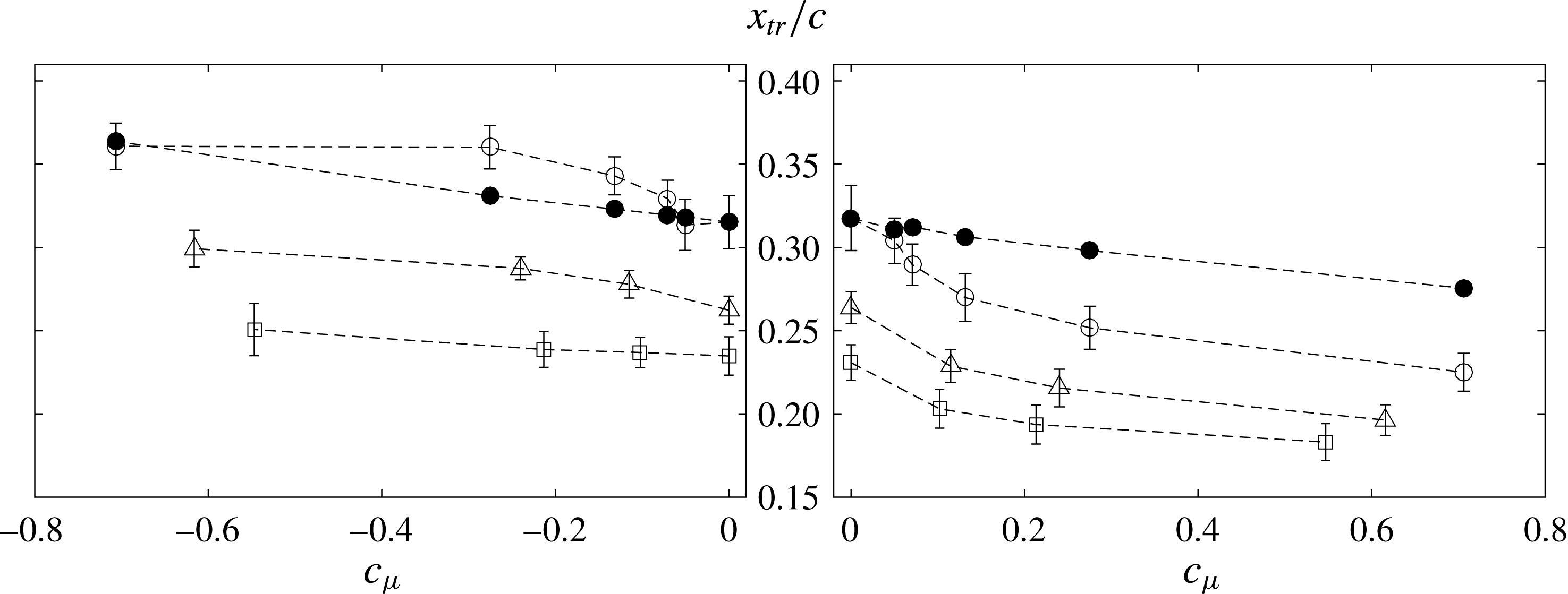
The aforementioned analysis can be extended to all tested cases, namely the variations in forcing momentum coefficient and Reynolds number. Experimentally measured transition locations extracted from the time-averaged IR fields are presented in figure 7, for both
 $-F_{x}$
and
 $F_{x}$
plasma forcing. Transition delay or advancement is proportional to the magnitude of
 $c_{\unicode[STIX]{x1D707}}$
.
Within the tested cases, the largest transition delay is approximately 4.5 %, occurring at the lowest Reynolds number and highest momentum coefficient tested. At higher Reynolds numbers, the displacement of the transition fronts with
 $c_{\unicode[STIX]{x1D707}}$
shows similar trends. For
 $Re_{c}=2.3\times 10^{6}$
(
 $U_{\infty }=27.5~\text{m}~\text{s}^{-1}$
) (▵),
 $c_{\unicode[STIX]{x1D707}}=-0.62$
and
 $Re_{c}=2.5\times 10^{6}$
(
 $U_{\infty }=30~\text{m}~\text{s}^{-1}$
) (▫),
 $c_{\unicode[STIX]{x1D707}}=-0.55$
the transition delay is 3.7 % and 1.6 %, respectively. The continuity in increasing the transition delay with
 $-c_{\unicode[STIX]{x1D707}}$
is well-defined; however, the percentage of delay decreases. Effectively, the current control technique is a direct approach against the weak CF velocity component. This component scales inviscidly with the free-stream velocity and thus, the authority of the applied body force on the boundary layer reduces as the Reynolds number increases (see variation of
 $c_{\unicode[STIX]{x1D707}}$
in figure 2
c).
Experimentally measured transition locations (
 $x_{tr}/c$
) versus momentum coefficient
 $c_{\unicode[STIX]{x1D707}}$
(○:
 $Re_{c}=2.1\times 10^{6}$
,
 $U_{\infty }=25~\text{m}~\text{s}^{-1}$
, ▵:
 $Re_{c}=2.3\times 10^{6}$
,
 $U_{\infty }=27.5~\text{m}~\text{s}^{-1}$
, ▫:
 $Re_{c}=2.5\times 10^{6}$
,
 $U_{\infty }=30~\text{m}~\text{s}^{-1}$
, ●: transition location predicted by the simplified numerical model for
 $Re_{c}=2.1\times 10^{6}$
,
 $U_{\infty }=25~\text{m}~\text{s}^{-1}$
).
Furthermore, the critical mode in the boundary layer changes with the Reynolds number (as predicted by LST, not shown here); however, the applied forcing is observed to still have an effect. This further demonstrates the inherent insensitivity of the base-flow modification strategy to the wavenumber of the stationary CFI modes, in contrast to the UFD/DRE approaches.
The uncertainty bands in figure 7 represent the width of the transition-front, estimated by the standard deviation of the jagged transition-front. The transition-front width observed here appears rather insensitive to the plasma forcing. A possible reduction in the transition-front width would suggest the amplification of travelling CFI modes in the boundary layer, as these modes blur the transition-front to a more spanwise uniform arrangement (Downs & White Reference Downs and White2013). This suggests that no fluctuations in the frequency band of travelling CFI modes were introduced, further confirming the recommendations of Serpieri et al. (Reference Serpieri, Yadala Venkata and Kotsonis2017) towards employing high AC driving frequencies.
The transition location for different
 $c_{\unicode[STIX]{x1D707}}$
predicted by the simplified model is also shown in figure 7. It is evident that the model is able to capture the experimental trend, but fails to predict the transition location accurately. This is expected, considering the range of assumptions and simplifications entering the chain of modelling steps (Serpieri et al.
Reference Serpieri, Yadala Venkata and Kotsonis2017). Notwithstanding the caveats brought forth, the simplified modelling approach presents a robust, fast and efficient tool, ideally suited for augmenting the experimental design process and providing basic, back-of-envelope scaling of the control performance.
4 Concluding remarks
The present study provides the first experimental proof of concept of plasma-based base-flow modification for CFI control. Nevertheless, several key points need to be addressed for the successful establishment of base-flow modification as a viable technique for the control of swept-wing boundary layers. A brief overview is given here. Cross-flow-dominated transition is known to be extremely sensitive to surface roughness effects (Saric et al. Reference Saric, Reed and White2003, Reference Saric, Carpenter and Reed2011, Reference Saric, West, Tufts and Reed2015). The DRE/UFD approach has shown promising results for control of CF-dominated transition; however, it also revealed the strong sensitivity of this technique to a number of parameters such as free-stream turbulence and background roughness (Lovig et al. Reference Lovig, Downs and White2014; Saric et al. Reference Saric, West, Tufts and Reed2015). While the base-flow modification strategy can be expected to be more robust to these effects, it also requires more energy to realise control of transition compared to the DRE/UFD strategy.
As mentioned earlier, any potential flow control system, aimed at swept-wing transition delay, needs to adhere to strict roughness and thickness thresholds. Although plasma actuators have been praised for their non-obtrusive character, conventional construction techniques typically followed in laboratory settings result in electrode thicknesses of tens of microns, which are prohibitive in the case of CF-dominated transition. In this study a prototype automated fabrication technique was developed to construct submicron metallic electrodes, which should be further developed, characterised and scaled. Furthermore, in Serpieri et al. (Reference Serpieri, Yadala Venkata and Kotsonis2017) plasma actuators were found to introduce velocity fluctuations in the band of travelling cross-flow instabilities. In the present study, the issue was circumvented by high AC driving frequency (
 $f_{ac}=10~\text{kHz}$
). However, upscaling this technique to higher Reynolds numbers will scale the frequency of instabilities as well. This will effectively require a further increase of the AC frequency, which will in turn challenge the current plasma generation approach. In addition, possible receptivity mechanisms between the plasma formation and incoming disturbances (i.e. free-stream turbulence) could give rise to the generation of secondary instabilities either through nonlinear interactions or transient growth. Dedicated studies of these mechanisms should be pursued.
A simplified numerical model was used to gain a preliminary handle on the expected control performance and confirm the working principle. Although the captured trends and order of magnitude for transition delay/advancement were satisfactory, ample room for improvement remains for such models, mainly in incorporating non-parallel and nonlinear theories. Notwithstanding the level of approximation, simple, fast and robust models are indispensable for the design of this type of control concept and experiment.
Finally, a key point is the future upscaling of the plasma forcing to higher Reynolds numbers. In the present study, the employed actuator was relatively weak and positioned in the simplest possible fashion (i.e. aligned to the leading edge in a straight line). Higher overall momentum coefficients can be achieved by increasing the dielectric thickness, applied voltage and number of successive actuators. Additionally, a technique enabled by the proposed automated electrode fabrication can be the use of curved electrodes, which follow the shape of the inviscid streamline, further optimising the forcing to fully counteract the CF component.
Acknowledgement
S.Y.V. is funded by the French Government programme ‘Investissements d’Avenir’ (LABEX INTERACTIFS, reference ANR-11-LABX-0017-01).


 Open access

