1. Introduction
Steep groups of surface gravity waves can arise from a variety of mechanisms, both linear and nonlinear. Frequency and directional dispersion can facilitate constructive interference between wave components (see, for example, Fedele et al. Reference Fedele, Brennan, De León, Dudley and Dias2016) while nonlinear wave–wave interactions alter the dispersive characteristics of a wave field allowing for self-focusing (Janssen Reference Janssen2003). Interactions with wind, current and bathymetry have been identified as further focusing mechanisms. Reviews by Kharif & Pelinovsky (Reference Kharif and Pelinovsky2003), Kharif, Pelinovsky & Slunyaev (Reference Kharif, Pelinovsky and Slunyaev2008b), Dysthe, Krogstad & Müller (Reference Dysthe, Krogstad and Müller2008) and Adcock & Taylor (Reference Adcock and Taylor2014) provide an extensive overview of steep wave formation and ‘rogue waves’. The characteristics of steep wave groups have been investigated in numerous previous studies, both in the context of random seas and isolated wave groups.
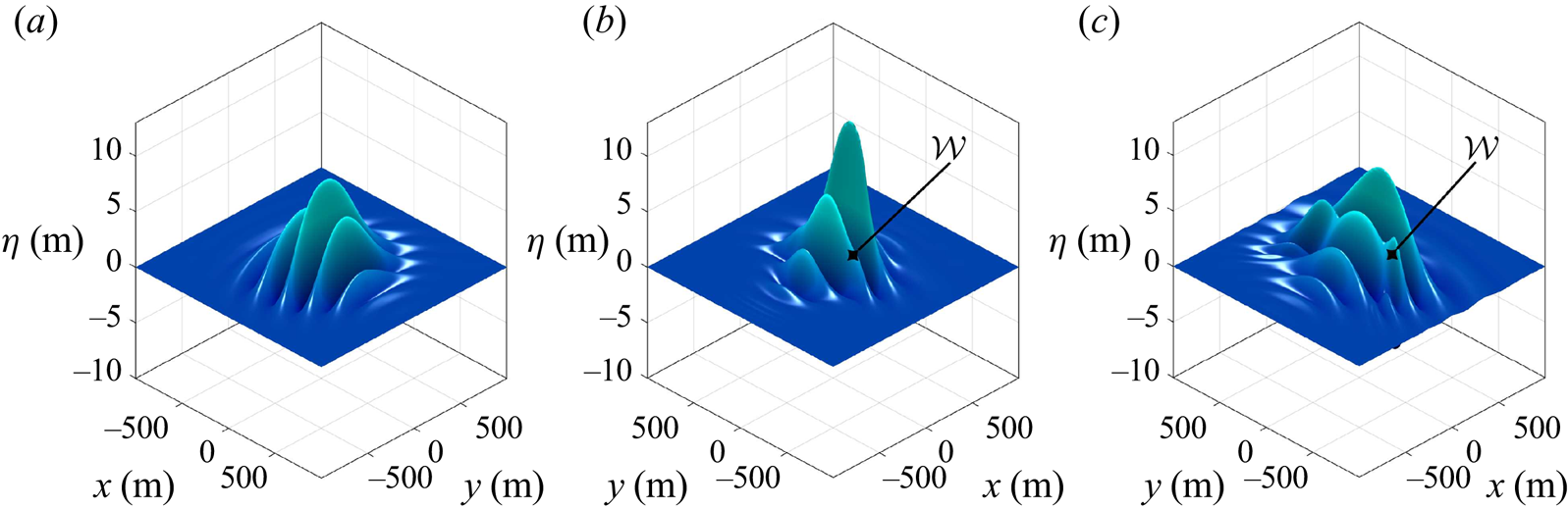
The random sea approach, characterised by an initially uniform phase distribution, captures the natural variability of wave focusing as well as interactions between neighbouring focused events and the global evolution of the background sea state. Steep wave events in a random sea have been found to exhibit front–rear asymmetry (Xiao et al. Reference Xiao, Liu, Wu and Yue2013; Adcock, Taylor & Draper Reference Adcock, Taylor and Draper2015; Fujimoto, Waseda & Webb Reference Fujimoto, Waseda and Webb2019), contraction in the direction of propagation (Adcock et al. Reference Adcock, Taylor and Draper2015) and a localised reduction in spreading at focus (Adcock et al. Reference Adcock, Taylor and Draper2015; Latheef, Swan & Spinneken Reference Latheef, Swan and Spinneken2017). Steep wave groups in a random sea have also been observed to exhibit a prolonged ‘lifetime’ due to nonlinear interactions (Fujimoto et al. Reference Fujimoto, Waseda and Webb2019). Random sea simulations and experiments are, however, innately inefficient because the vast majority of the observed wave events are not particularly steep. An alternative approach based on isolated wave groups has thus been pursued by previous studies, characterised by a coherent phase distribution designed to focus wave components in time and space. This is less computationally expensive, allows error waves associated with low-order numerical wave paddles or initial conditions to be easily identified and discounted (since the error waves separate out from the main group) and highlights changes in group shape. The wave–wave interactions which arise for an isolated wave group are driven by the same physical processes as those of a random sea, and we use the isolated wave group approach in this study. Numerical simulations of isolated wave groups performed by Gibbs & Taylor (Reference Gibbs and Taylor2005) as well as Gibson & Swan (Reference Gibson and Swan2007) reported ‘rapid’ changes to the underlying wave spectrum, altering the amplitude and phase speed of the resonant components, and attributed the spectral changes to third-order resonant interactions. Barratt et al. (Reference Barratt, Bingham and Adcock2020) used the potential flow code OceanWave3D to simulate focusing wave groups, depicted before focus in figure 1(a), at nonlinear focus in figure 1(b), and after focus in figure 1(c). Directional energy transfers were found to cause the formation of ‘wing waves’, localised oblique protrusions at the periphery of the wave group marked with  $\mathcal {W}$ in figure 1. The formation of wing waves has been attributed by Barratt et al. (Reference Barratt, Bingham and Adcock2020) to third-order resonant interactions. Thus, previous studies indicate that third-order resonant interactions influence the characteristics of steep wave groups formed by dispersive focusing.
Surface elevation ( $\eta$) of a steep wave group formed by dispersive focusing, simulated by Barratt, Bingham & Adcock (Reference Barratt, Bingham and Adcock2020) with OceanWave3D: (a) pre-focus,
 $t/T_0=-7.5$; (b) nonlinear focus,
 $t/T_0=1.3$; (c) post-focus,
 $t/T_0=7.5$. Times are defined relative to the linear focus time, normalised by the characteristic period (
 $T_0$). The formation of ‘wing waves’, localised regions of elevation due to energised oblique components, is demarcated with
 $\mathcal {W}$. These results have been compared against the higher-order spectral (HOS) simulations of Gibbs & Taylor (Reference Gibbs and Taylor2005); the maximum surface elevation agrees within 0.3 % with total energy conservation within 0.024 % over 40 wave periods.

Third-order resonance for deep-water waves has been shown by Phillips (Reference Phillips1960) to occur between four wave components that satisfy the conditions
 \begin{equation} \boldsymbol{k}_{1}\pm\boldsymbol{k}_{2}\pm\boldsymbol{k}_{3}\pm\boldsymbol{k}_{4}=0, \end{equation}
and with the same combination of signs,
 \begin{equation} {\omega_{1}}\pm{\omega_{2}}\pm{\omega_{3}}\pm{\omega_{4}}=\delta\omega, \end{equation}
consistent with the deep-water linear dispersion relationship,
 \begin{equation} {\omega_{i}}^{2}=g{k_{i}}. \end{equation}
Here, the wavenumber and angular frequency of each component are denoted with  $\boldsymbol {k}_i$ and
 $\omega _i$, respectively. The gravitational constant is denoted with
 $g$, and
 $\delta \omega$ represents an angular frequency mismatch which detunes the interaction. Resonant interactions can be categorised as either exactly resonant, if
 $\delta \omega$ is strictly zero, or nearly resonant, if
 $\delta \omega$ is
 $O(\epsilon ^{2}\omega _0)$, based on a characteristic frequency (
 $\omega _0$). As discussed by Stiassnie (Reference Stiassnie2017), the Zakharov equation accounts for exactly and nearly resonant quartets, with an associated dynamic time scale of
 $O(\epsilon ^{-2}T_0)$, based on the characteristic time scale of the wave field (
 $T_0$). In contrast, the Hasselmann (Reference Hasselmann1962) equation only accounts for exactly resonant quartets, with an associated kinetic time scale of
 $O(\epsilon ^{-4}T_0)$. A quartet of interacting wave components is termed ‘degenerate’ if only three unique wave components are involved – one of the components participates twice in the interaction (e.g.
 $\boldsymbol {k}_{1}=\boldsymbol {k}_{2}$). Degenerate quartet interactions form the basis of stability analyses for a regular/monochromatic wave. In this study, we consider the role of degenerate interactions in the spectral evolution of narrow-banded focusing wave groups. Previous studies indicate that quartet interactions are particularly prevalent for narrow-banded wave fields and wave fields which are ‘out of equilibrium’, both of which are considered in this study.
Narrow-banded wave fields have been a particular focus of previous studies due to their large third-order interactions. Longuet-Higgins (Reference Longuet-Higgins1976) investigated the resonant interactions of a narrow-banded wave spectrum, using the Davey & Stewartson (Reference Davey and Stewartson1974) equation, and calculated a resonance angle of  $\arctan {(\pm 1/\sqrt {2})}=\pm 35.26^{\circ }$ relative to the spectral peak. Notably, the angle calculated by Longuet-Higgins (Reference Longuet-Higgins1976) matches the resonance angle of the Phillips (Reference Phillips1960) ‘figure-of-eight’ loop for a degenerate quartet and the instability region of the
 $2+1$ nonlinear Schrödinger equation (NLS) equation, as calculated by Zakharov (Reference Zakharov1968), Benney & Roskes (Reference Benney and Roskes1969) and Davey & Stewartson (Reference Davey and Stewartson1974). Crawford et al. (Reference Crawford, Lake, Saffman and Yuen1981) used the Zakharov equation to investigate the stability of a wave train to three-dimensional modulations and observed instability bands contained within the Phillips resonance loop. The eigenvalue stability analysis of McLean (Reference McLean1982b) also revealed quartet instability bands within the Phillips resonance loop for a finite-amplitude regular wave and showed that the dominant quartet instabilities are unidirectional in deep water. Alber (Reference Alber1978) performed a stability analysis, based on the Davey & Stewartson (Reference Davey and Stewartson1974) equation, and found that a homogeneous spectrum of random waves is unstable to oblique inhomogeneous disturbances at angles less than
 ${\pm }35.26^{\circ }$ if the bandwidth is sufficiently narrow but becomes stable for broader bandwidths. Conversely, Stuhlmeier & Stiassnie (Reference Stuhlmeier and Stiassnie2017) observed evidence of instability for broad-banded spectra subject to small inhomogeneous disturbances, using a discretised version of the Zakharov equation without bandwidth limits. In this study, our simulations of narrow-banded wave groups exhibit directional energy transfers which resemble the Philips resonance loop for a degenerate quartet. However, as the wave group becomes more broad-banded we observe other directional energy transfers not encompassed by the Phillips resonance loop. We discuss the impact of the spectral evolution on the shape, kinematics and lifespan of the wave groups and assess the effects of steepness, finite depth, directional spreading and the high-wavenumber tail.
Spectral equilibrium is another factor which has been linked by previous studies to the importance of third-order interactions. The role of wave-field equilibrium in the formation of extreme waves has been highlighted by Trulsen (Reference Trulsen, Velarde, Tarakanov and Marchenko2018); sudden changes in water depth and meteorological conditions were identified as possible causes for non-equilibrium. Random wave fields which are ‘out of equilibrium’ are expected to evolve on the dynamic  $O(\epsilon ^{-2}T_0)$ time scale, as discussed by Annenkov & Shrira (Reference Annenkov and Shrira2006) and Annenkov & Shrira (Reference Annenkov and Shrira2018). Onorato & Suret (Reference Onorato and Suret2016) identified wind, current and topography and factors which can bring a wave field out of equilibrium. As noted by Trulsen (Reference Trulsen, Velarde, Tarakanov and Marchenko2018), random wave-field simulations initialised with artificial spectra exhibit rapid spectral evolution during the early stages of the simulation (see, e.g., Dysthe et al. Reference Dysthe, Trulsen, Krogstad and Socquet-Juglard2003; Socquet-Juglard et al. Reference Socquet-Juglard, Dysthe, Trulsen, Krogstad and Liu2005; Toffoli et al. Reference Toffoli, Onorato, Bitner-Gregersen and Monbaliu2010; Xiao et al. Reference Xiao, Liu, Wu and Yue2013). A similar effect has been observed experimentally by Shemer, Sergeeva & Liberzon (Reference Shemer, Sergeeva and Liberzon2010) for waves generated from an artificial spectrum in a laboratory tank. Gramstad & Trulsen (Reference Gramstad and Trulsen2007) performed modified nonlinear Schrödinger (MNLS) simulations based on the equation of Trulsen & Dysthe (Reference Trulsen and Dysthe1996) and found that the occurrence of freak waves relates to crest and group length, highlighting the role of spectral bandwidth and spreading. The theory of wave turbulence associates nonlinear interactions (and non-Gaussian properties) with intermittency and Fadaeiazar et al. (Reference Fadaeiazar, Alberello, Onorato, Leontini, Frascoli, Waseda and Toffoli2018) found that directional spreading reduces intermittency also indicating that spreading may be an important feature of spectral equilibrium. Various early studies have furthered the discussion of wave-field equilibrium, including: the wind speed investigation of Waseda, Toba & Tulin (Reference Waseda, Toba and Tulin2001), the NLS simulations of Onorato et al. (Reference Onorato, Osborne, Serio and Bertone2001), the wave turbulence study of Onorato et al. (Reference Onorato, Osborne, Serio, Resio, Pushkarev, Zakharov and Brandini2002), the kurtosis evolution analysis of Janssen (Reference Janssen2003) and the phase-resolved stochastic analysis of Stiassnie & Shemer (Reference Stiassnie and Shemer2005). In this study, we perform simulations based on Gaussian as well as Joint North Sea Wave Project (JONSWAP) spectra, with different spreading functions, and consider the role of directional spreading and the high-wavenumber tail in spectral equilibrium for steep wave groups formed by dispersive focusing.
In summary, we perform numerical simulations of narrow-banded wave groups, formed by dispersive focusing, using a fully nonlinear potential flow code. We investigate the rapid spectral evolution due to third-order interactions and assess the effects of steepness, finite depth, directional spreading and the tail of the spectrum. We also consider the implications of third-order interactions for the shape, lifetime and kinematics of the wave groups, as well as the implications for wave loads acting on a column. Our simulations indicate that the directional energy transfers of a narrow-banded wave group initially resemble the Phillips resonance loop but agreement deteriorates as the wave group becomes more broad-banded. We also observe that the localised nonlinear features of an individual steep wave event may depend on the spectral equilibrium of the underlying sea state.
2. Details of the numerical simulations
We perform numerical simulations with the fully nonlinear potential flow code OceanWave3D, described in Engsig-Karup, Bingham & Lindberg (Reference Engsig-Karup, Bingham and Lindberg2009). Time marching of the initial conditions has been performed both excluding and including the nonlinear terms in the free-surface boundary conditions. The linear and nonlinear simulations begin with identical amplitudes and phases for the wave components, highlighting the influence of wave–wave interactions. We use the method of phase separation (Fitzgerald et al. Reference Fitzgerald, Taylor, Eatock Taylor, Grice and Zang2014) to remove the bound harmonics from the nonlinear simulations, isolating the free wave components.
2.1. Initial conditions
We prescribe the initial conditions in terms of surface elevation,  $\eta (x,y,t)$, and velocity potential at the free surface,
 $\tilde {\phi }(x,y,t)$, calculated 15 characteristic wave periods before the time of linear focus. Time is thus defined relative to the linear focus time (
 $t/T_{0}=0$), and the free-surface quantities time marched for 30 wave periods, terminating the simulation 15 wave periods after the linear focus time. Typical of the North Sea, the initial peak of the wavenumber spectrum for all simulations is located at
 $k_p=0.02796\ \textrm {m}^{-1}$, which corresponds to a characteristic wavelength (
 $\lambda _{0}$) of 225 m and characteristic wave period (
 $T_{0}$) of 12.0–12.8 s for depths in the range of 48.7–200 m.
The variance density spectrum  $F(k,\theta )$ of the initial conditions has been defined as the product of a wavenumber magnitude spectrum
 $S(k)$ and a spreading function
 $D(\theta )$. Two types of wavenumber magnitude spectra are considered in this study, a Gaussian spectrum:
 \begin{equation} {S}(k)={S_0}\exp{\left(\frac{-(k-k_p)^{2}}{2{k_w}^2}\right)}, \end{equation}
and a JONSWAP spectrum with  $\gamma =3.3$ (Hasselmann et al. Reference Hasselmann, Barnett, Bouws, Carlson, Cartwright, Enke, Ewing, Gienapp, Hasselmann and Kruseman1973). The coefficient
 $S_0$ of (2.1) is taken to be unity since the focused amplitude of the wave event is determined by
 $A_L$ in (2.3). The JONSWAP spectrum represents a realistic spectrum for fetch-limited seas. Here,
 $k_{p}$ denotes the wavenumber corresponding to the initial peak of the wavenumber spectrum and
 $k_{w}$ represents the bandwidth of the Gaussian spectra. A value of
 $k_{p}=0.02796\ \textrm {m}^{-1}$ has been used for both the Gaussian and JONSWAP spectra and a bandwidth of
 $k_{w}=0.004606\ \textrm {m}^{-1}$ has been used for all the Gaussian cases. The Gaussian spectra have been calculated from three bandwidths below the spectral peak (
 $k=k_{p}-3k_{w}$) to three bandwidths above the spectral peak (
 $k=k_{p}+3k_{w}$) and the JONSWAP spectrum has been calculated up to
 $k/k_p=10$ based on the resolution of the grid in the OceanWave3D simulations. Note that the Gaussian wavenumber magnitude spectrum used in the study closely approximates the shape of the spectral peak for a JONSWAP spectrum with
 $\gamma =3.3$.
Two different spreading functions have been implemented in this study: a frequency-independent Gaussian spreading function
 \begin{equation} D(\theta)=\frac{1}{\varsigma_{0}\sqrt{2{\rm \pi}}}\exp{\left({\frac{-\theta^{2}}{2{\varsigma_{0}^{2}}}}\right)}, \end{equation}
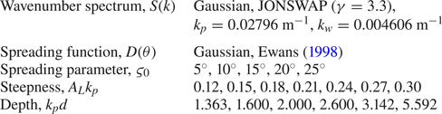
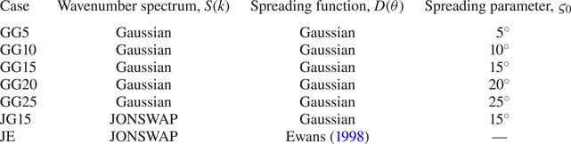
and the frequency-dependent spreading function of Ewans (Reference Ewans1998). The Gaussian spreading function includes an initial spreading parameter ( $\varsigma _{0}$) listed in table 1 for the various test cases. The Ewans (Reference Ewans1998) spreading function has been selected to account for the oblique angle of high-wavenumber components in the tail of the spectrum frequently observed in the field measurements of fetch-limited seas as described by Banner & Young (Reference Banner and Young1994), Hwang et al. (Reference Hwang, Wang, Walsh, Krabill and Swift2000), Leckler et al. (Reference Leckler, Ardhuin, Peureux, Benetazzo, Bergamasco and Dulov2015) and Peureux, Benetazzo & Ardhuin (Reference Peureux, Benetazzo and Ardhuin2018).
Parameter space of initial conditions.

Quasi-determinism theory, based on Boccotti (Reference Boccotti1983) and Lindgren (Reference Lindgren1970) (see Boccotti (Reference Boccotti2000) for a comprehensive review), indicates that the average shape of an extreme event in a random, linear Gaussian field is the scaled auto-correlation function, used in this study to calculate the initial conditions of the extreme wave groups. The wave field is, thus, spatially inhomogeneous, and the linear surface elevation of the wave group,  $\eta (x,y,t)$, is given by
 \begin{equation} \eta(x,y,t)={A_{L}}\frac{\sum_{i,j}{F(k_{i},\theta_{j}) \cos{(k_{i}\cos{\theta_{j}}x+k_{i}\sin{\theta_{j}}y-\omega_{i}{t}+ \varphi_{0})}}}{\sum_{i,j}{F(k_{i},\theta_{j})}}. \end{equation}
Here,  $k_{i}$ is the magnitude of the wavenumber for each component,
 $\theta _{i}$ is the direction of propagation,
 $A_{L}$ is the linear amplitude of the wave group at focus (
 $t/T_{0}=0$) and the angular frequency of each component (
 $\omega _{i}$) is calculated from the arbitrary-depth linear dispersion relationship,
 $\omega _{i}=\sqrt {gk_{i}\tanh {(k_{i}d)}}$. Table 1 lists the linear steepnesses of the simulated wave groups as well as the dimensionless depths, both based on the initial peak of the wavenumber spectrum
 $k_{p}$. The phase offset (
 $\varphi _0$) is required for the four-phase separation technique (Fitzgerald et al. Reference Fitzgerald, Taylor, Eatock Taylor, Grice and Zang2014) used to remove bound harmonics from the wave spectrum; we have performed the simulations with phase offsets of
 $0^{\circ }$,
 $90^{\circ }$,
 $180^{\circ }$,
 $270^{\circ }$ for every case, which allows the free harmonics to be approximately separated from the bound harmonics. We apply exact second-order corrections to the initial conditions based on the formulation of Dalzell (Reference Dalzell1999) together with an approximate form of third-order correction based on Barratt et al. (Reference Barratt, Bingham and Adcock2020). Note that we evaluate the second-order terms of Dalzell (Reference Dalzell1999) at the mean water level but we evaluate the linear terms at the free surface to minimise the formation of second-order error waves.
2.2. Code description and simulation fidelity
OceanWave3D discretises the potential flow equations for surface gravity waves in a three-dimensional spatial domain using Cartesian coordinates ( $x,y,z$). The code is based upon an Eulerian frame of reference and cannot capture overturning waves. A non-conformal transform is used to map the solution to a time-invariant domain comprised of structured rectilinear grids
 \begin{equation} \sigma\equiv\frac{z+d(x,y)}{\eta(x,y,t)+d(x,y)}, \end{equation}
and uniform depth,  $d(x,y)=d$, in this study. Classic fourth-order Runge–Kutta time marching combined with finite differencing of the spatial derivatives yields a linear system of equations, solved with the generalised minimum residual (GMRES) algorithm. Left preconditioning is performed once every iteration with multi-grid Gauss–Seidel relaxation. The multi-grid scheme is based on direct coarse grid approximation and follows a ‘V-cycle’, descending from the finest grid resolution down to the coarsest grid resolution before ascending again from the coarsest grid resolution to the finest grid resolution, with one pre-smoothing and one post-smoothing step. We apply a relative tolerance of
 $10^{-6}$ for convergence of the GMRES algorithm at each time step.
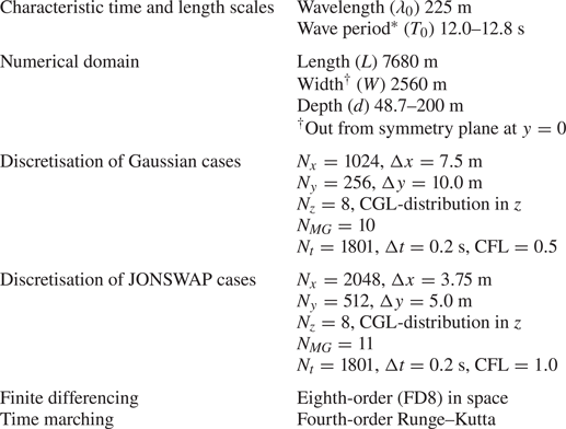
The grid-convergence study of Barratt et al. (Reference Barratt, Bingham and Adcock2020), based on grid halving in all three spatial dimensions, informs our selection of the grid resolution. The size of the numerical domain is listed in table 2, indicating the length ( $L$) in the x-direction, width (
 $W$) in the y-direction and depth (
 $d$) in the vertical, z-direction. The length and width of the domain are fixed for all simulations. However, we vary the depth of the domain. The horizontal grid distribution (
 ${\rm \Delta} {x}$,
 ${\rm \Delta} {y}$) is uniform throughout the domain. We utilise a symmetry plane along the centreline of the wave group (
 $y=0$). Thus, the width of the domain listed in table 2 only represents half of the effective domain width. The position of the symmetry plane results in asymmetric stencils along the centre of the wave group. However, by performing simulations with and without a symmetry plane, Barratt et al. (Reference Barratt, Bingham and Adcock2020) confirmed that the additional numerical diffusion due to the asymmetric stencils is negligible. We use powers of two for the number of grids (
 $N_{x}$,
 $N_{y}$,
 $N_{z}$) in all three spatial dimensions, to ensure the maximum number of multi-grid levels (
 $N_{MG}$) for the preconditioning scheme. The number of grids in the horizontal directions (
 $N_{x}$,
 $N_{y}$) has been doubled for the JONSWAP cases, compared with the Gaussian cases, to better resolve the smaller-wavelength components in the tail of the JONSWAP spectrum.
Numerical details of OceanWave3D simulations.

We use eighth-order finite differencing, confirmed by Barratt et al. (Reference Barratt, Bingham and Adcock2020) to exhibit a grid-independent iteration count for simulations similar to those of this study. Central-differencing schemes have been used, except at the boundaries, and the order of finite differencing is consistent throughout. We include a single layer of ghost nodes, outside the domain of interest, for all surfaces except the free surface. The presence of ghost nodes at the bottom boundary allows both continuity and the Neumann boundary condition to be simultaneously satisfied while improving the numerical stability of the preconditioning scheme, even for anisotropic grid distributions in the vertical direction. Thus, we use the symmetric half of a Chebyshev–Gauss–Lobatto (CGL) distribution in the vertical direction:  $\sigma _{j}=\sin {(({\rm \pi} [\,j-1])/(2[N_{z}-1]))}$, where
 $j$ denotes the index of the grid point with
 $j=1$ at the bottom and
 $j=N_{z}$ at the free surface. The time step size, based on the Courant–Friedrichs–Lewy (CFL) condition, influences diffusion error but not dispersion error. Thus, we use the same time step for the JONSWAP and Gaussian cases based upon the permissible levels of diffusivity, resulting in CFL values of 1.0 and 0.5 respectively.
2.3. Spectral parameters
We analyse the spectral evolution of the various simulations performed in this study in terms of moments of the wavenumber–amplitude spectrum as well as spreading bandwidth. We also consider the wave action density spectrum to determine the time scales of energy transfer between wave components. The zeroth moment of the discrete wavenumber–amplitude spectrum ( $\mathcal {M}_{0}$)
 \begin{equation} \mathcal{M}_{0}=\sum_{i}|\hat{\eta}(k_{i},\theta_i)|, \end{equation}
represents a summation of amplitudes for the Fourier components of surface elevation in the discrete wavenumber spectrum,  $\hat {\eta }(k_{i},\theta _{i})$, and thus represents the amplitude of the wave which would be formed by perfect constructive interference between all wave components. For linear evolution,
 $\mathcal {M}_{0}$ in (2.5) equals
 $A_{L}$ as defined in (2.3) for the entirety of the simulation. The zeroth spectral moment
 $\mathcal {M}_{0}$ can be expected to increase as energy transfers in a narrow-banded spectrum lead to broadening of the spectrum. We use the first moment of the wavenumber–amplitude spectrum
 \begin{equation} \mathcal{M}_{1}=\sum_{i}{k_{i}}|\hat{\eta}(k_{i},\theta_i)|, \end{equation}
normalised by the zeroth spectral moment ( $\mathcal {M}_{0}$) to define a mean wavenumber (
 $\mathcal {K}$)
 \begin{equation} \mathcal{K}=\mathcal{M}_{1}/\mathcal{M}_{0}. \end{equation}
The mean wavenumber  $\mathcal {K}$ increases if high-wavenumber components grow in amplitude while low-wavenumber components diminish in amplitude. Thus,
 $\mathcal {K}$ increases if energy transfer from low-wavenumber components to high-wavenumber components prevails and decreases in the opposite scenario. We also consider the root-mean-square (RMS) spreading (
 $\varsigma$)
 \begin{equation} \varsigma=\sqrt{\frac{\sum_{i}{\theta_{i}}^{2}|\hat{\eta}(k_{i},\theta_i)|}{\mathcal{M}_{0}}}, \end{equation}
which quantifies the bandwidth of directional spreading. Note that the initial value of (2.8) matches the parameter  $\varsigma _{0}$ in (2.2) if the frequency-independent Gaussian spreading function is used. The spectral parameters defined in (2.7) and (2.8) have been evaluated for both the Gaussian and JONSWAP cases based on wavenumber components in the range:
 $0<k_x/k_p\leq 2$ and
 $-2\leq k_y/k_p \leq 2$. We restrict the calculation to the vicinity of the spectral peak to assess the Gaussian spectrum as a model for the peak of a JONSWAP spectrum. Thus, we do not include the full tail of the JONSWAP spectrum in the calculation of the spectral parameters. However, we note that the considered range of wavenumbers accounts for 96 %–98 % of the total energy for the JONSWAP cases, calculated at every time step for each simulation.
The total wave action of a wave group is a conserved quantity (see Komen et al. Reference Komen, Cavaleri, Donelan, Hasselmann, Hasselmann and Janssen1994), and the spectrum of wave action density has been calculated from the amplitude spectrum to quantify the component growth rates. The energy density spectrum  $E({k_i},\theta _{i})$, associated with the amplitude spectrum of surface elevation in wavenumber space, has been calculated based upon the amplitude of each Fourier component,
 $a_i$, and the discrete wave number intervals (
 ${\rm \Delta} k_{x},{\rm \Delta} k_{y}$) together with the density of water (
 $\rho$)
 \begin{equation} E({k_{i}})=\frac{\frac{1}{2}\rho g a_i^{2}}{{\rm \Delta} k_{x}{\rm \Delta} k_{y}}. \end{equation}
Using the linear dispersion relation, the wave action density spectrum is given by
 \begin{equation} A({k_{i}})=\frac{E({k_{i}})}{\omega_{i}}, \end{equation}
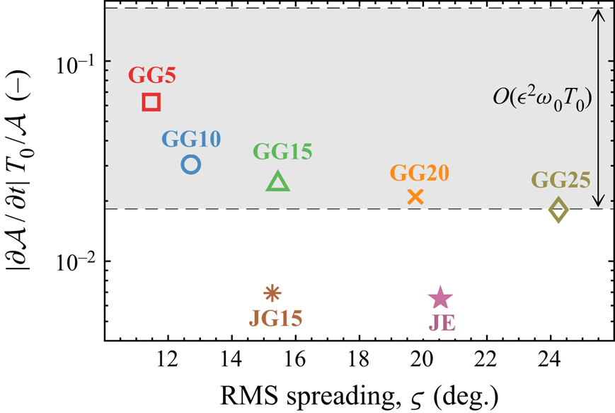
In this study, we consider the growth rate of specific wave components. For context, Stiassnie (Reference Stiassnie2001) notes that the growth rate associated with the Hasselmann equation is
 \begin{equation} {[{\partial \mathcal{A}({k_i},\theta_{i})}/{\partial t}]}{T_0}\big/{\mathcal{A}({k_i}, \theta_{i})}=O(\epsilon^{4}\omega_{0}{T_0}), \end{equation}
where  $\omega _{0}$ represents the characteristic wave period, and the growth rate associated with the Zakharov equation is
 \begin{equation} {[{\partial \mathcal{A}({k_i},\theta_{i})}/{\partial t}]}{T_0}\big/{\mathcal{A} ({k_i},\theta_{i})}=O(\epsilon^{2}\omega_{0}{T_0}).\end{equation}
3. Results and discussion
We begin our analysis with a base case, followed by an investigation of steepness, finite-depth, directional spreading and the high-wavenumber tail of the spectrum.
3.1. Directional energy transfers due to third-order interactions
The selected base case features a Gaussian wavenumber spectrum with a Gaussian spreading function and a spreading parameter ( $\varsigma$) of
 $15^{\circ }$, denoted as case ‘GG15’. We prescribe a linear steepness (
 $A_{L}k_{p}$) of 0.3 for the base case at the linear focus time (
 $t/T_0=0$), from (2.3), together with a dimensionless depth (
 $k_{p}d$) of 3.142. Results are shown for the linear version of the base case, in which the nonlinear terms of the free-surface boundary conditions are neglected, and the fully nonlinear version of the base case which includes all terms in the free-surface boundary conditions. Figure 1 shows the surface elevation corresponding to the nonlinear version of the base case, including the wing waves (demarcated with
 $\mathcal {W}$) which form as a result of directional energy transfers.
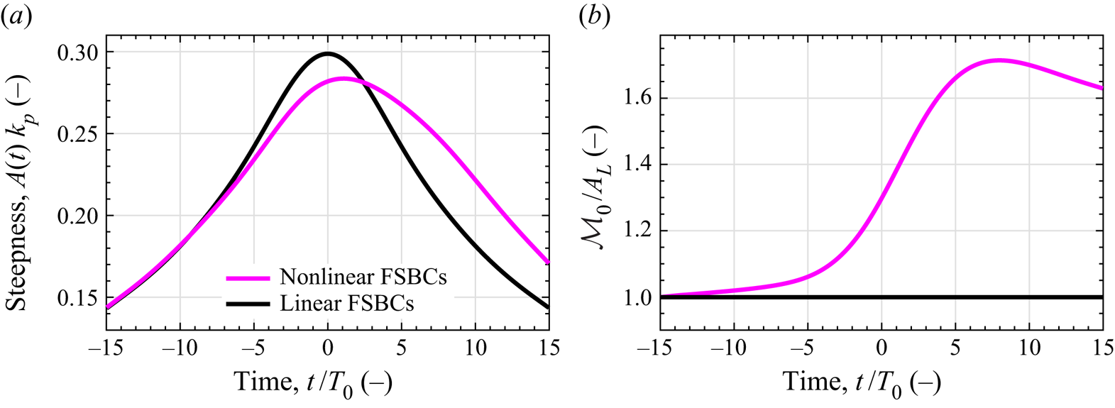
The steepness of the wave envelope over time ( $A(t)k_{p}$) is shown in figure 2(a) for both the linear and nonlinear version of the base case. As expected, the linear envelope is symmetric about the focal time. However, the nonlinear envelope exhibits asymmetry about
 $t/T_{p}=0$ due to nonlinear wave–wave interactions which modify the amplitude and dispersion of the wave components, extending the life span of this focused wave event. Nonlinear interactions are known to alter the phase speed of the participating wave components, which can counteract dispersion and preserve the form of a focused wave event – the competing effects of nonlinearity and dispersion is a central idea to the Benjamin–Feir index (see Janssen Reference Janssen2003). Figure 2(b) shows the zeroth spectral moment of the amplitude spectrum (
 $\mathcal {M}_{0}$), normalised by the linear focus amplitude (
 $A_{L}$). For linear evolution, the ratio equals unity at all times. However, for nonlinear evolution the zeroth moment can be seen to increase during the focusing of the wave group reaching a maximum value of
 ${\mathcal {M}_{0}}/A_{L}=1.7$ at
 $t/T_0=8.0$ in figure 2(b). Although the zeroth moment increases continuously during the wave focusing event, the amplitude of the nonlinear event at focus is smaller than the amplitude of the linear event due to modifications in phase speed. For the linear simulation, the phase of each component has been selected to ensure perfect constructive interference at
 $t/T_0=0$. For the nonlinear simulation, nonlinear dispersion prevents perfect constructive interference at focus. Thus, the steepness of the focused event is reduced, despite the increase in zeroth moment shown in figure 2(b). Although the spectral evolution of the nonlinear event does not increase the amplitude of the wave envelope in this case, the wave–wave interactions significantly alter the shape of the wave group and the magnitude of the wave kinematics, discussed in § 3.2. Adjusting the initial phase of the wave components could evidently result in a nonlinear event which is locally larger than the linear version of the event.
Comparison for case GG15 with linear and nonlinear free-surface boundary conditions (FSBCs), a steepness of  $A_{L}k_{p}=0.3$ and a dimensionless depth of
 $k_{p}d=3.142$. (a) Steepness of the wave envelope over time. The amplitude
 $A(t)$ is based on the maximum elevation of the wave envelope at time
 $t$. The linear case is represented by the black line (thick black) and the nonlinear case is represented by the magenta line (thick magenta). (b) The zeroth moment of the wavenumber–amplitude spectrum (
 $\mathcal {M}_{0}$) normalised by the linear focus amplitude (
 $A_{L}$). The dimensionless ratio is plotted over time for the nonlinear case (thick magenta) and the linear case (thick black). For the linear case, the ratio
 $\mathcal {M}_{0}/A_{L}$ equals unity at all instances in time.

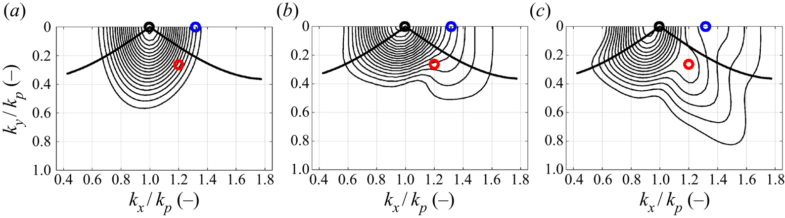
For the base case, we also consider the evolution of the wave spectrum due to nonlinear wave–wave interactions, calculated with a discrete Fourier transform of the wave group surface elevation. Figure 3 depicts contour plots of the amplitude spectrum in wavenumber space for: the initial condition,  $t/T_{0}=-15$; the time of nonlinear focus,
 $t/T_{0}=1.3$; and the end of the simulation,
 $t/T_{0}=15$. Segments of the Phillips ‘figure-of-eight’ resonance loop are also shown. The initial condition in figure 3(a) is narrow-banded and remains narrow-banded during the early stages of focusing due to the low steepness of the initially dispersed wave group. However, evolution of the amplitude spectrum occurs as the wave group steepens and approaches focus, see figure 2. In particular, energy transfer to high-wavenumber components is evident in figure 3(b), with a directional bias qualitatively consistent with the Phillips resonance loop, at angles of
 ${\pm }35.26^{\circ }$ to the spectral peak, accompanied by unidirectional energy transfers along the
 $k_{x}$-axis. A low-wavenumber sidelobe can be seen at nonlinear focus in figure 3(b), although the footprint is considerably smaller than the high-wavenumber sidelobe. The spectral changes observed in figure 3(b) are, thus, reminiscent of the Class I instability band for a regular wave train of finite amplitude, described by McLean (Reference McLean1982b), and we attribute the spectral changes to ‘quasi-degenerate’ interactions. A degenerate quartet is comprised of only three unique wave components (since one component participates twice,
 $\boldsymbol {k}_{1}=\boldsymbol {k}_{2}$) and forms the basis of stability analyses for a regular/monochromatic wave, assuming that
 $\boldsymbol {k}_{1}$ and
 $\boldsymbol {k}_{2}$ both equate to the characteristic wavenumber
 $\boldsymbol {k}_{0}$ of the regular wave. Phillips (Reference Phillips1960) showed that the interacting components of a degenerate quartet form the ‘figure-of-eight’ resonance loop, and the eigenvalue stability analysis of McLean (Reference McLean1982b) indicates that the instability band of a finite-amplitude regular wave includes components on the
 $k_{x}$-axis if the water is deep. In this study, we consider narrow-banded wave spectra which form focused wave groups. The concentration of energy around the spectral peak means that we anticipate interactions in which
 $\boldsymbol {k}_{1}$ and
 $\boldsymbol {k}_{2}$ resemble the characteristic wavenumber
 $\boldsymbol {k}_{0}$ (wavenumber of the initial spectral peak) but may not strictly equate. Thus, we expect
 $\boldsymbol {k}_{1}\approx \boldsymbol {k}_{2}\approx \boldsymbol {k}_{0}$ for our narrow-banded wave groups, rather than
 $\boldsymbol {k}_{1}=\boldsymbol {k}_{2}=\boldsymbol {k}_{0}$ as expected for a regular/monochromatic wave. Interactions of the form
 $\boldsymbol {k}_{1}\approx \boldsymbol {k}_{2}$ are not strictly degenerate. Thus, we use the term ‘quasi-degenerate’ to describe quartet interactions with
 $\boldsymbol {k}_{1}\approx \boldsymbol {k}_{2}$. Despite the resemblance of the directional energy transfers figure 3(b) to the Phillips resonance loop, it seems improbable that all the directional energy transfers in figure 3(b) are the result of exactly degenerate quartets, due to the strict definition. Thus, we attribute the directional energy transfers evident in 3(b) to quasi-degenerate interactions since the definition of quasi-degenerate interactions is more relaxed and encompasses a large number of interactions with resonance loops that resemble the classic Phillips resonance loop. After nonlinear focus, figure 3(c), the amplitude spectrum continues to broaden with directional energy transfer to high-wavenumber components not encompassed by the Phillips resonance loop. Divergence from the figure-of-eight is likely due to the degenerate nature of the resonance loop. Broadening of the spectrum during focusing, thus, appears to facilitate non-degenerate interactions (
 $\boldsymbol{k}_{1}{\neq}\,\boldsymbol{k}_{2}$) after focus, resulting in high-angle oblique energy transfers along a
 ${\pm }55^{\circ }$ angle. Notably, there are spectral changes which arise during focus that do not reverse after focus indicating permanent changes to the spectrum. We note that suppressed linear dispersion has been observed by Steer et al. (Reference Steer, Borthwick, Onorato, Chabchoub and van den Bremer2019) for modulations which propagate at
 ${\pm }35.26^{\circ }$ to the wave group, which can increase the lifetime of a focused wave event. Thus, the
 ${\pm }35.26^{\circ }$ energy transfers apparent in figure 3(b) may contribute to the lifetime extension depicted in figure 2(a). The formation of a high-wavenumber sidelobe has also been associated by Adcock & Taylor (Reference Adcock and Taylor2016) with contraction of the wave group in the direction of propagation. The amplitude spectrum at nonlinear focus also exhibits a contraction of the spectrum along the
 $k_{y}$-direction, which implies lateral expansion of the wave group and a focused wave event which is less directionally spread than the initial wave spectrum.
Discrete amplitude spectra of surface elevation corresponding to case GG15 with a steepness of  $A_{L}k_{p}=0.3$ and a dimensionless depth of
 $k_{p}d=3.142$: (a) initial condition,
 $t/T_{0}=-15$; (b) nonlinear focus,
 $t/T_{0}=1.3$; (c) post-focus,
 $t/T_{0}=15$. Contour levels (black solid line) are evenly distributed between 0.01 and 0.105 m in intervals of 0.005 m. The thick black line (thick black) represents a segment of the Phillips ‘figure-of-eight’ resonance loop and the open circles specify particular wavenumber components for further analysis:
 $\mathcal {Q}$ (thick black circle)
 $k_{x}/k_{p}=0.995$,
 $k_{y}/k_{p}=0.000$;
 $\mathcal {R}$ (thick red circle)
 $k_{x}/k_{p}=1.200$,
 $k_{y}/k_{p}=0.263$;
 $\mathcal {S}$ (thick blue circle)
 $k_{x}/k_{p}=1.317$,
 $k_{y}/k_{p}=0.000$.

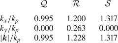
Three specific components in the wavenumber spectrum ( $\mathcal {Q}$,
 $\mathcal {R}$,
 $\mathcal {S}$) have been selected for further analysis of the growth rate – the components are shown in figure 3 and listed in table 3. Component
 $\mathcal {Q}$ coincides with the initial peak of the wavenumber spectrum, component
 $\mathcal {S}$ denotes a component on the
 $k_x$-axis, in the instability band of a finite-amplitude regular wave train, and component
 $\mathcal {R}$ coincides with the local maximum of the oblique ridge at
 ${\pm }55^{\circ }$ formed by non-degenerate interactions.
Wavenumber components selected for growth analysis shown in figure 3.

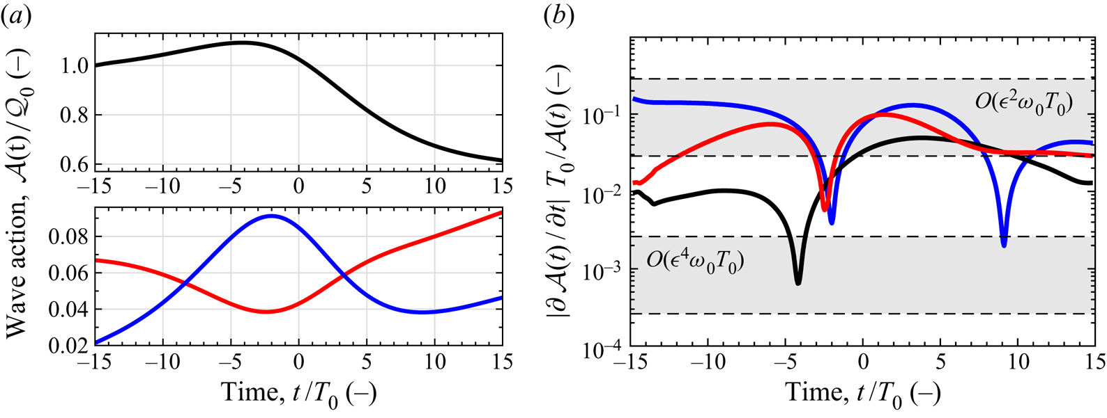
Figure 4(a) shows the wave action density of the three components. Before focus, the wave action density of component  $\mathcal {Q}$ grows, indicating energy transfer to the spectral peak, while the wave action density of component
 $\mathcal {R}$ declines, due to contraction of the spectrum in the
 $k_{y}$-direction, and component
 $\mathcal {S}$ grows, due to energy transfers to higher wavenumbers. Before nonlinear focus occurs at
 $t/T_{0}=1.3$, the wave action density of component
 $\mathcal {Q}$ begins to decline, signalling the onset of a downshift in the spectral peak, and component
 $\mathcal {R}$ begins to grow, continuing to grow for the remainder of the simulation. Component
 $\mathcal {S}$ reaches a maximum in wave action density before nonlinear focus and thereafter begins to decline, which is likely a result of spectral broadening inhibiting quasi-degenerate interactions. Previous work by Longuet-Higgins (Reference Longuet-Higgins1978), McLean (Reference McLean1982b), Francius & Kharif (Reference Francius and Kharif2003) and Fedele (Reference Fedele2014) has also demonstrated the suppression of unidirectional instabilities at high wave steepnesses, which may also constrain the growth in wave action density for component
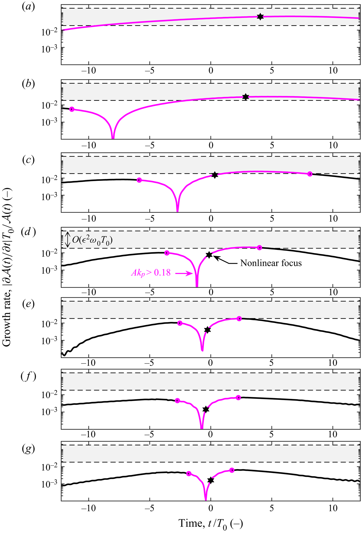
 $\mathcal {S}$ during focus. The corresponding dimensionless growth rates for the three components (
 $\mathcal {Q}$,
 $\mathcal {R}$,
 $\mathcal {S}$) are shown in figure 4(b) in terms of wave action density. For context, the dynamic time scale associated with near resonance and the Zakharov equation,
 $O(\epsilon ^2 \omega _0 T_0)$, is shown together with the kinetic time scale associated with exact resonance and the Hasselmann equation,
 $O(\epsilon ^4 \omega _0 T_0)$.
Component-wise analysis of the wave action density spectrum for case GG15 with a steepness of  $A_{L}k_{p}=0.3$ and a dimensionless depth of
 $k_{p}d=3.142$: (a) the wave action density of each component over time, normalised by the initial wave action density of the spectral peak (
 $\mathcal {Q}_{0}$); (b) the non-dimensional growth rate of each component over time, plotted on a logarithmic ordinate. The components correspond to those indicated in figure 3:
 $\mathcal {Q}$ (thick black)
 $k_{x}/k_{p}=0.995$,
 $k_{y}/k_{p}=0.000$;
 $\mathcal {R}$ (thick red line)
 $k_{x}/k_{p}=1.200$,
 $k_{y}/k_{p}=0.263$;
 $\mathcal {S}$ (thick blue line)
 $k_{x}/k_{p}=1.317$,
 $k_{y}/k_{p}=0.000$. The dynamic growth rate
 $O(\epsilon ^{2}\omega _{0}T_{0})$ and the kinetic growth rate
 $O(\epsilon ^{4}\omega _{0}T_{0})$ are indicated by bounded (bold dashed line) grey bands. The value of
 $\epsilon$ equates to
 $A_{L}k_{p}/{\rm \pi}$ in the growth rate calculations.

Similar results to figure 3 have been observed by Adcock & Taylor (Reference Adcock and Taylor2016) using the MNLS equation of Trulsen & Dysthe (Reference Trulsen and Dysthe1996). Thus, these spectral changes can be attributed to resonant third-order interactions, since the MNLS equation is only capable of resolving third-order/four-wave interactions, as demonstrated by Stiassnie (Reference Stiassnie1984). Furthermore, the HOS simulations of Gibbs & Taylor (Reference Gibbs and Taylor2005) were performed with a truncated form of Dirichlet–Neumann operator and yielded results similar to figure 3; the authors indicated that a comparison of third-order and fifth-order simulations produced no significant variations. Thus, the fourth-order Class II instabilities observed by McLean (Reference McLean1982b) do not appear to be significant for the simulated wave groups in this study. Although the present study is focused on isolated wave groups, the oblique energy transfers and consequent spectral evolution shown in figure 3 qualitatively resemble previous random sea results (e.g. Dysthe et al. Reference Dysthe, Trulsen, Krogstad and Socquet-Juglard2003; Socquet-Juglard et al. Reference Socquet-Juglard, Dysthe, Trulsen, Krogstad and Liu2005; Toffoli et al. Reference Toffoli, Onorato, Bitner-Gregersen and Monbaliu2010; Xiao et al. Reference Xiao, Liu, Wu and Yue2013; Simanesew et al. Reference Simanesew, Krogstad, Trulsen and Nieto Borge2016, Reference Simanesew, Krogstad, Trulsen and Nieto Borge2018). Toffoli et al. (Reference Toffoli, Onorato, Bitner-Gregersen and Monbaliu2010), for example, used HOS simulations to demonstrate that a random wave field initialised with frequency-independent spreading develops frequency-dependent spreading resembling figure 3. The simulations of Toffoli et al. (Reference Toffoli, Onorato, Bitner-Gregersen and Monbaliu2010) did not include external forcing, such as wind and breaking, and the spectral evolution can thus be attributed to nonlinear wave–wave interactions. Simanesew et al. (Reference Simanesew, Krogstad, Trulsen and Nieto Borge2016) performed laboratory experiments and MNLS simulations initialised with frequency-independent spreading and also observed the development of frequency-dependent spreading. Dynamic nonlinear contributions to the development of frequency-dependent spreading, above and below the spectral peak, were identified, consistent with our observations. Simanesew et al. (Reference Simanesew, Krogstad, Trulsen and Nieto Borge2018) investigated wave spectra based on field measurements from the North Sea and MNLS simulations, using different data-adaptive methods and indicate that frequency-dependent spreading can be a numerical artefact of ‘peak splitting’ by maximum entropy methods. However, Simanesew et al. (Reference Simanesew, Krogstad, Trulsen and Nieto Borge2018) conclude that the development of frequency-dependent spreading in the spectral tail does also result from nonlinear wave–wave interactions, consistent with our results. Thus, the local spectral evolution surrounding steep wave events, featuring oblique energy transfers away from the spectral peak, may contribute to the global evolution of the underlying sea-state. The development of frequency-dependent spreading does, however, occur slower for the background sea state of a random sea requiring hundreds of wave periods to fully develop. In contrast, significant frequency-dependent spreading develops within 30 wave periods in the present study of steep wave groups.
3.2. Implications of spectral changes for kinematics and loads
The spectral changes observed in figure 3 are relevant to the kinematics of the wave group. The wave loads acting upon a vertical cylinder can be calculated with the Morison equation, see for example Paulsen et al. (Reference Paulsen, Bredmose, Bingham and Jacobsen2014), yielding the horizontal force
 \begin{equation} F={\int_{-d}^{\eta}}\frac{1}{2}{C_{D}\rho{A}u(z){|u(z)|}\,\textrm{d} z+ {\int_{-d}^{\eta}}{C_{M}}\rho{V}{\frac{\textrm{D} u(z)}{\textrm{D} t}}}\textrm{d} z, \end{equation}
featuring a drag term with a quadratic dependency on the horizontal velocity,  $u{|u|}$, and an inertial term proportional to the Lagrangian acceleration of the horizontal velocity,
 ${\textrm {D} u}/{\textrm {D} t}$, defined in terms of the material derivative. Here,
 $u(z)$ represents the characteristic horizontal velocity which may vary in the vertical,
 $z$-direction. Constants
 $C_D$ and
 $C_M$ depend on geometry and Reynolds number. The frontal area of the body (
 $A$) as well as the volume (
 $V$) are required for the calculation, together with the density of the fluid (
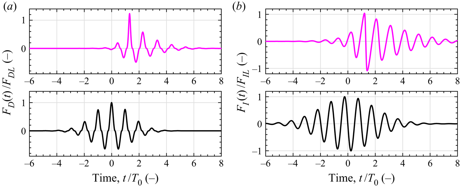
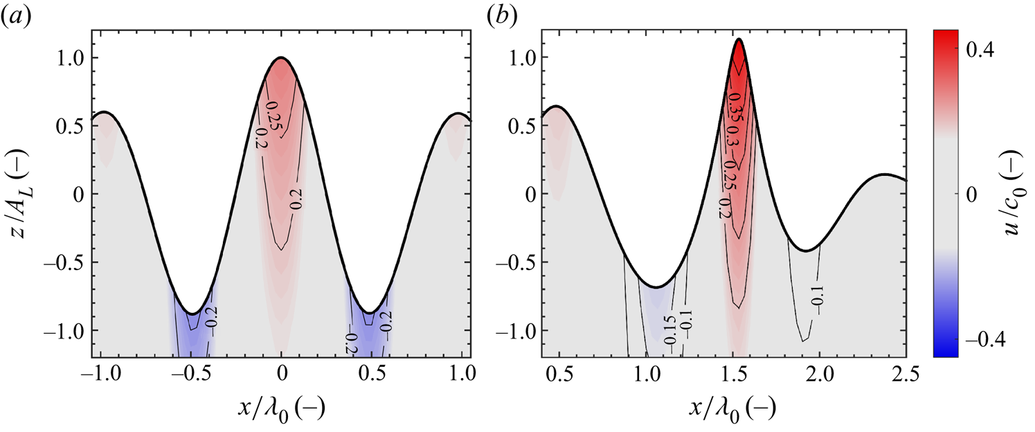
 $\rho$). Energy transfers to higher wavenumbers augments both the velocities and accelerations of the wave field, increasing both the drag and inertial loads as estimated by the Morison equation. Furthermore, the reduction in directional spreading shown in 3(b), which occurs during focusing, increases the in-line velocity component and thus increases the horizontal velocity component used in (3.1). We have calculated (3.1) for both the linear and nonlinear versions of the base case. A time history of the force, at the spatial location where focus occurs, is plotted for both the linear and nonlinear cases – the drag term is shown in figure 5(a) and the inertial term is shown in figure 5(b). Separate axes are used in figure 5 for the linear and nonlinear cases for clarity. The nonlinear case exhibits higher drag and inertial forces at focus than the linear case as a result of energy transfers to higher wavenumbers and the reduced spreading of the nonlinear focused event. The maximum drag and inertial forces are, respectively, 24 % and 4 % higher for the nonlinear case, compared with the linear case. The shape of the linear and nonlinear focused events is shown in figure 6 with contours of the in-line velocity component (
 $u$), aligned to the
 $x$-direction, and normalised by the phase speed associated with the spectral peak (
 $c_0$). The linear event depicted in figure 6(a) exhibits front–rear symmetry, and the height of the crest is comparable to the depth of the preceding and trailing troughs; a peak in-line velocity of
 $u/c_0=0.294$ arises in the crest of the linear focused event. For the nonlinear event depicted in figure 6(b), front–rear asymmetry is apparent as the preceding trough is shallower than the trailing trough. The surface elevation includes bound harmonics which result in a higher crest and shallower troughs than observed for the linear event; a peak in-line velocity of
 $u/c_0=0.449$ arises in the crest of the nonlinear focused event, 53 % higher than the linear case. The particle image velocimetry experiments of Alberello et al. (Reference Alberello, Chabchoub, Monty, Nelli, Lee, Elsnab and Toffoli2018) are consistent with the numerical simulation results shown in figure 6. Alberello et al. (Reference Alberello, Chabchoub, Monty, Nelli, Lee, Elsnab and Toffoli2018) observed that unidirectional wave groups, formed by dispersive focusing, contract in the direction of propagation and exhibit asymmetric features consistent with figure 6: a preceding trough that is shallower than the trailing trough and a focused crest that is sharper than both the preceding and trailing trough. The consequent kinematics measured by Alberello et al. (Reference Alberello, Chabchoub, Monty, Nelli, Lee, Elsnab and Toffoli2018) featured concentrated high-velocity regions in the crest, similar to figure 6, associated with the onset of breaking. Note that a variety of breaking criteria have been proposed based on crest kinematics/energy fluxes (see, e.g., Barthelemy et al. (Reference Barthelemy, Banner, Peirson, Fedele, Allis and Dias2018)) and neither of the focused events shown in figure 6 are expected to break (see Perlin, Choi & Tian (Reference Perlin, Choi and Tian2013) for a review of breaking criteria). In summary, the spectral evolution observed in the base case GG15 results in augmented kinematics and loads, demonstrating the significance of nonlinear interactions.
Time history of force calculated from the terms of the Morison equation for case GG15 with a steepness of  $A_{L}k_{p}=0.3$ and a dimensionless depth of
 $k_{p}d=3.142$: (a) drag force corresponding to the
 $u|u|$ term of the Morison equation – the force has been normalised by the maximum drag force of the linear case
 $F_{DL}$; (b) inertial force corresponding to the
 $\partial {u}/\partial {t}$ term of the Morison equation – the force has been normalised by the maximum inertial force of the linear case
 $F_{IL}$. The linear case is depicted by the black line (thick black) and the nonlinear case is depicted by the magenta line (thick magenta). The time history of force is calculated at the spatial location where focus of the wave group occurs:
 $x/\lambda _{0}=0$,
 $y/\lambda _{0}=0$ for the linear case and
 $x/\lambda _{0}=1.535$,
 $y/\lambda _{0}=0$ for the nonlinear case, by integrating from the bottom of the domain (
 $z=-d$) to the surface elevation (
 $z=\eta$).

Internal kinematics at the time of focus for case GG15 with a steepness of  $A_{L}k_{p}=0.3$ and a dimensionless depth of
 $k_{p}d=3.142$. (a) Linear evolution, focus occurs at
 ${t/T_{0}=0}$; (b) nonlinear evolution, focus occurs at
 $t/T_{0}=1.3$. The spatial coordinate in the direction of propagation (x-direction) is shown on the horizontal axis and the vertical spatial coordinate (z-direction) is shown on the vertical axis. The horizontal velocity in the direction of wave group propagation (u-velocity) is shown beneath the surface elevation (thick black) of the wave group, normalised by the phase speed associated with the initial peak of the wavenumber spectrum (
 $c_0$). Labelled contour lines of the dimensionless velocity ratio
 $u/c_0$ are shown in the figures together with a colour bar of the same parameter.

3.3. Steepness, finite-depth and directional spreading effects
Following our analysis of the base case, we investigate the effects of steepness, finite depth and directional spreading on spectral evolution on the mean wavenumber ( $\mathcal {K}$) and the spreading parameter (
 $\varsigma$).
3.3.1. Steepness
We assess the effect of amplitude for wave groups based on a Gaussian wavenumber spectrum and a Gaussian spreading function with an initial spreading parameter ( $\varsigma _0$) of
 $15^{\circ }$ and a dimensionless depth of
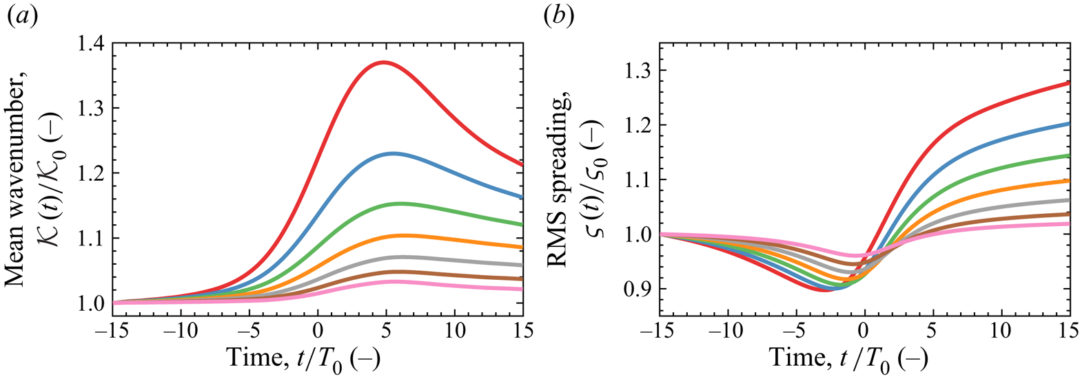
 $k_p d=3.142$. The linear steepness at focus is varied between 0.12 and 0.30 in intervals of 0.03. The mean wavenumber, defined in (2.7), and spreading parameter, defined in (2.8), are shown in figure 7. The vertical axis of both plots is normalised by the initial value of the parameter. The evolution in mean wavenumber, shown in figure 7(a), depicts an increase during focus with a rate dependent upon steepness. The increase during focus is predominantly due to the quasi-degenerate interactions, discussed in § 3.1, which result in energy transfers to higher wavenumbers. After focus, the mean wavenumber peaks and thereafter declines for all cases. The post-focus decline in mean wavenumber is due to the post-focus dominance of the non-degenerate interactions discussed in § 3.1 – the high oblique angle components possess a smaller absolute wavenumber than those along the unidirectional
 $k_{x}$-axis, thereby decreasing the mean wavenumber. Figure 7(b) shows the corresponding evolution of the spreading parameter (
 $\varsigma$), which exhibits a qualitatively similar trend for all steepnesses. The spreading parameter initially declines during focusing, indicating a more unidirectional wave group resembling the ‘wall of water’ effect described by Gibbs & Taylor (Reference Gibbs and Taylor2005) and observed experimentally by Steer et al. (Reference Steer, Borthwick, Onorato, Chabchoub and van den Bremer2019), followed by a rapid increase in directional spreading due to the oblique non-degenerate energy transfers shown in figure 3(c). The increase in directional spreading occurs earlier for the steeper wave groups indicating an earlier onset of the non-degenerate interactions.
Spectral evolution over time for case GG15 with different linear steepnesses ( $A_{L}k_{p}$) and a dimensionless depth of
 $k_{p}d=3.142$: (a) mean wavenumber
 $\mathcal {K}(t)$ normalised by the initial value
 $\mathcal {K}_{0}$; (b) RMS spreading parameter
 $\varsigma (t)$ normalised by the initial value
 $\varsigma _{0}$. The various steepnesses are indicated by colour:
 $A_{L}k_{p}=0.30$, thick red;
 $0.27$, thick blue;
 $0.24$, thick green;
 $0.21$, thick orange;
 $0.18$, thick grey;
 $0.15$, thick brown;
 $0.12$, thick pink.

3.3.2. Finite depth
The effect of finite depth has also been assessed for wave groups based on a Gaussian wavenumber spectrum and a Gaussian spreading function with an initial spreading parameter ( $\varsigma _0$) of
 $15^{\circ }$ and a linear steepness (
 $A_{L}k_{p}$) of 0.30, with the results shown in figure 8. The considered range of depth spans from
 $k_p{d}=5.592$ to
 $k_p{d}=1.363$; a depth of
 $k_p{d}=3.142$ is frequently considered to be ‘deep water’, and the lower bound of
 $k_p{d}=1.363$ is significant as the critical depth of vanishing modulational instability for unidirectional waves (see Benjamin Reference Benjamin1967; Whitham Reference Whitham1967). However, Benney & Roskes (Reference Benney and Roskes1969) and McLean (Reference McLean1982a) showed that unstable three-dimensional perturbations remain for depths less than
 $k_p{d}=1.363$, consistent with our findings – we observe suppressed nonlinear evolution of the wave spectrum for a depth of
 $k_p{d}=1.363$ but rapid energy transfers evidently do still occur.
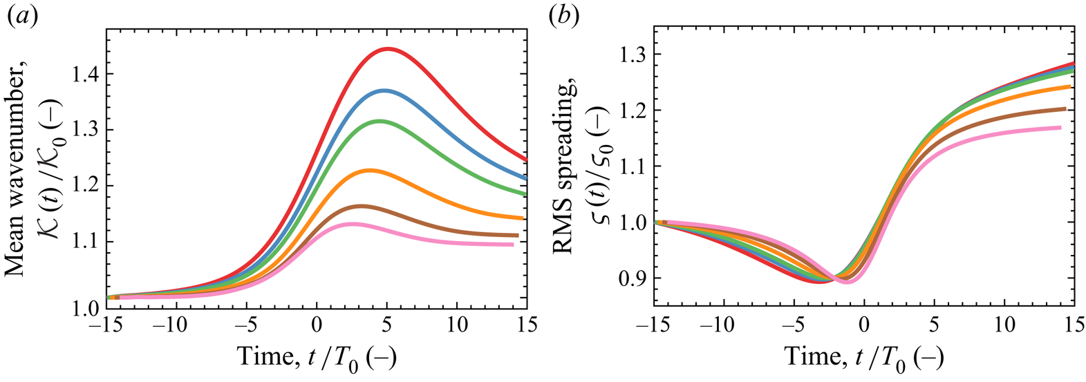
Spectral evolution over time for case GG15 with different dimensionless depths ( $k_{p}d$) and a steepness of
 $A_{L}k_{p}=0.3$: (a) mean wavenumber
 $\mathcal {K}(t)$ normalised by the initial value
 $\mathcal {K}_{0}$; (b) RMS spreading parameter
 $\varsigma (t)$ normalised by the initial value
 $\varsigma _{0}$. The various depths are indicated by colour:
 $k_{p}d=5.592$, thick red;
 $k_{p}d=3.142$, thick blue;
 $k_{p}d=2.600$, thick green;
 $k_{p}d=2.000$, thick orange;
 $k_{p}d=1.600$, thick brown;
 $k_{p}d=1.363$, thick pink.

Figure 8(a) depicts the evolution of the mean wavenumber, normalised by the initial value, for various finite depths. A reduction in depth suppresses the increase in mean wavenumber observed during focus but a discernible increase remains apparent for  $k_p{d}=1.363$. We also observe sensitivity to depth between
 $k_p{d}$ values typically considered to represent ‘deep water’. Depths of
 $k_p{d}=5.592$ and
 $k_p{d}=3.142$ result in peak
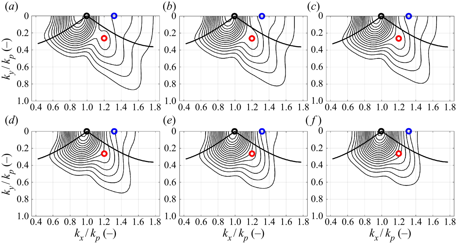
 $\mathcal {K}(t)/\mathcal {K}_0$ values of 1.44 and 1.37, respectively. Figure 9 shows the amplitude spectrum of surface elevation at the end of the simulation (
 $t/T_0=15$) for the various finite-depth cases. The case of
 $k_p{d}=5.592$ depicted in figure 9(a) exhibits greater energy transfers along the unidirectional
 $k_x$-axis and the Phillips resonance loop than observed for the
 $k_p{d}=3.142$ case shown in figure 9(b). Thus, the quasi-degenerate interactions appear to be depth sensitive even in water typically considered to be deep; the observation can be explained by the interplay between the modulation instability and the return current as found by Benjamin (Reference Benjamin1967) and Whitham (Reference Whitham1974) and discussed by Dysthe (Reference Dysthe1979) and Janssen & Onorato (Reference Janssen and Onorato2007). The return current develops beneath the wave group with a length scale comparable to the wave group as a whole. Thus, the return current is more sensitive to depth than any individual wave component and, as observed in this study, can be altered by depths greater than
 $k_p{d}=3.142$. The return current is also capable of ‘detuning’ the modulational instability. Thus, the sensitivity of the return current to depth appears to influence the quasi-degenerate interactions observed in this study, altering the nonlinear wave–wave interactions of cases
 $k_p{d}=5.592$ and
 $k_p{d}=3.142$.
Amplitude spectra of surface elevation at the end of the simulation,  $t/T_{0}=15$, corresponding to case GG15 with a steepness of
 $A_{L}k_{p}=0.3$ and various dimensionless depths: (a)
 $k_{p}d=5.592$; (b)
 $k_{p}d=3.142$; (c)
 $k_{p}d=2.600$; (d)
 $k_{p}d=2.000$; (e)
 $k_{p}d=1.600$; (f)
 $k_{p}d=1.363$. Contour levels (black solid line) are evenly distributed between 0.01 and 0.105 m in intervals of 0.005 m. The thick black line (thick black) represents segments of the Phillips ‘figure-of-eight’ resonance loop and the open circles specify particular wavenumber components:
 $\mathcal {Q}$ (thick black circle)
 $k_{x}/k_{p}=0.995$,
 $k_{y}/k_{p}=0.000$;
 $\mathcal {R}$ (thick red circle)
 $k_{x}/k_{p}=1.200$,
 $k_{y}/k_{p}=0.263$;
 $\mathcal {S}$ (thick blue circle)
 $k_{x}/k_{p}=1.317$,
 $k_{y}/k_{p}=0.000$.

In contrast, the spreading parameter shown in figure 8(b) is less significantly affected by depth. The reduction in directional spreading, observed during focus, achieves a similar minimum value for all the finite-depth cases, although the less deep cases exhibit a delay compared with the deeper cases. The delay is expected because the increase in directional spreading is associated with spectral broadening due to quasi-degenerate interactions. Thus, suppression of the quasi-degenerate interactions by depth delays the onset of non-degenerate interactions. The increase in directional spreading, which dominates the wavenumber spectrum after focus, exhibits only a weak sensitivity to depth with an almost identical spreading parameter at the end of the simulation for finite depths ( $k_p{d}$) of
 $5.592$,
 $3.142$ and
 $2.600$. The relative insensitivity of the spreading parameter to depth, compared with the mean wavenumber, appears to result from differing depth sensitivity for the quasi-degenerate and non-degenerate interactions discussed in § 3.1. As demonstrated by figure 9, the quasi-degenerate interactions which transfer energy along the unidirectional
 $k_x$-axis and the Phillips resonance loop exhibit a clear sensitivity to depth and continuously weaken for less deep cases, almost disappearing for the case of
 $k_{p}d=1.363$. In contrast, the non-degenerate interactions, which develop once the wave spectrum is sufficiently broad-banded and transfer energy at an angle of
 ${\pm }55^{\circ }$ to the spectral peak, are significantly less affected by depth. The oblique energy transfers at
 ${\pm }55^{\circ }$ are suppressed by depth but continue to dominate the spectral evolution even for
 $k_{p}d=1.363$. Consequently, the mean wavenumber is sensitive to energy transfers to higher wavenumbers by the quasi-degenerate interactions and, thus, exhibits depth sensitivity. The spreading parameter is principally governed by the oblique energy transfers of the non-degenerate interactions and, thus, exhibits less sensitivity to depth.
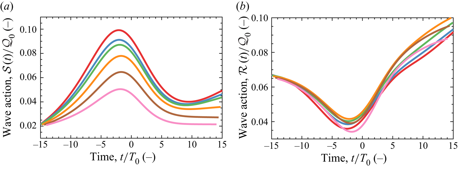
We have also analysed the change in wave action density for components  $\mathcal {R}$ and
 $\mathcal {S}$ with the results shown in figure 10. Normalisation is performed with the initial wave action density of the spectral peak (
 $\mathcal {Q}_0$). The wave action density of component
 $\mathcal {S}$, shown in figure 10(a), depicts a qualitatively similar trend for all the depth cases but demonstrates suppressed energy transfers at reduced depths. In contrast, component
 $\mathcal {R}$ depicts a similar quantitative trend in wave action density for all depths and even exhibits faster growth for finite-depth cases
 $k_pd=2.000$ and
 $k_pd=1.600$ than the deep-water cases. Benney & Roskes (Reference Benney and Roskes1969) and McLean (Reference McLean1982a) showed that the peak instability of a regular wave train becomes oblique, rather than unidirectional, at intermediate depths. Thus, the faster growth rate for component
 $\mathcal {R}$ observed for cases
 $k_pd=2.000$ and
 $k_pd=1.600$ may be a result of the quasi-degenerate interactions biasing towards oblique rather than unidirectional components. Ultimately, depth suppresses all forms of spectral evolution in the intermediate range of depths (
 $5.592>k_{p}{d}>1.363$) considered by this study, consistent with the finite-depth random sea simulations of Toffoli et al. (Reference Toffoli, Benoit, Onorato and Bitner-Gregersen2009). However, unidirectional energy transfers appear to be particularly suppressed relative to the oblique energy transfers. Thus, the increase in mean wavenumber is suppressed, which suggests less severe wave kinematics. However, the reduction in directional spreading, observed during focus, appears to occur for all the finite-depth cases suggesting that the ‘wall of water’ effect may also be observed in waters of intermediate depth, consistent with the experiments of Latheef et al. (Reference Latheef, Swan and Spinneken2017). The interplay between the return current and modulation instability also results in depth sensitivity within the range of depths commonly considered to be ‘deep’, suggesting that the length scale of the return current and wave group are of greater significance than the length scale of individual wave components when categorising water as ‘deep’.
Change in wave action density corresponding to case GG15 with a steepness of  $A_{L}k_{p}=0.3$ and various dimensionless depths:
 $k_{p}d=5.592$, thick red;
 $k_{p}d=3.142$, thick blue;
 $k_{p}d=2.600$, thick green;
 $k_{p}d=2.000$, thick orange;
 $k_{p}d=1.600$, thick brown;
 $k_{p}d=1.363$, thick pink. The analysis has been performed for specific wavenumber components: (a) component
 $\mathcal {S}$ (
 $k_{x}/k_{p}=1.317$,
 $k_{y}/k_{p}=0.000$); (b) component
 $\mathcal {R}$ (
 $k_{x}/k_{p}=1.200$,
 $k_{y}/k_{p}=0.263$); both components are normalised by the initial wave action density of the spectral peak (
 $\mathcal {Q}_0$), and the location of the components in the wavenumber spectrum is shown in figure 9.

3.3.3. Directional spreading
We consider the effects of directional spreading for wave groups with a linear steepness ( $A_{L}k_{p}$) of 0.24 based on a Gaussian wavenumber magnitude spectrum with a Gaussian spreading function and a finite depth (
 ${k_{p}}{d}$) of 3.142. Our simulations include initial spreading parameters (
 $\varsigma {}_{0}$) in the range of
 $5^{\circ }$ to
 $25^{\circ }$ in intervals of
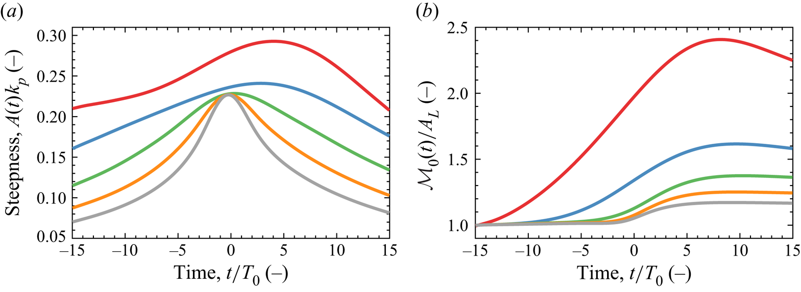
 $5^{\circ }$. Focused wave events with high values of directional spreading exhibit a reduced focal time, compared with less spread or unidirectional events, due to linear dispersion. Figure 11(a) shows the steepness of the wave envelope for the various cases of directional spreading. As can be seen, the less spread cases, e.g.
 $\varsigma _0=10^{\circ }$, begin with a higher steepness and steepen gradually until focus. In contrast, the cases with more directional spreading, e.g.
 $\varsigma _0=25^{\circ }$, begin with a lower steepness and steepen rapidly before focus. Directional spreading, thus, reduces the focal time of the wave event, limiting the total energy transfer in an integral sense. Figure 11(a) also demonstrates the influence of nonlinear interactions on the life span of the focused wave events. Under linear evolution, each case should focus and defocus symmetrically, see figure 2. However, cases
 $\varsigma _0=5^{\circ }$ and
 $\varsigma _0=10^{\circ }$ exhibit deviations between focusing and defocusing due to nonlinear interactions, extending the life span of the focused events.
Effect of directional spreading for wave groups with a steepness of  $A_{L}k_{p}=0.24$, finite depth of
 $k_{p}d=3.142$ and initial spreading parameters of
 $5^{\circ }$ (thick red),
 $10^{\circ }$ (thick blue),
 $15^{\circ }$ (thick green),
 $20^{\circ }$ (thick orange) and
 $25^{\circ }$ (thick grey). (a) Steepness of the wave envelope over time – the amplitude
 $A(t)$ is based on the maximum elevation of the wave envelope at time
 $t$; (b) the zeroth moment of the wavenumber–amplitude spectrum (
 $\mathcal {M}_{0}$) normalised by the linear focus amplitude (
 $A_{L}$). All cases are based on a Gaussian wavenumber spectrum with a Gaussian spreading function.

The spectral evolution is also demonstrated by figure 11(b), which shows the zeroth moment of the amplitude spectrum ( $\mathcal {M}_{0}$), normalised by the linear amplitude at focus (
 $A_{L}$), for all the spreading cases. Under linear evolution,
 $\mathcal {M}_{0}=A_{L}$ throughout the simulation. Under nonlinear evolution, an increase in
 $\mathcal {M}_{0}$ indicates a transition from a narrow-banded to a more broad-banded spectrum. The zeroth moment increases drastically for the
 $\varsigma _0=5^{\circ }$ case due to rapid broadening of the spectrum. Consequently, the focused wave event is significantly steeper than the linear steepness, and the lifespan of the event is extended. In contrast, the
 $\varsigma _0=25^{\circ }$ case depicts a nearly constant zeroth moment until shortly before focus, indicating less spectral broadening during focus, which results in a steepness and focused lifespan which resembles the linear event.
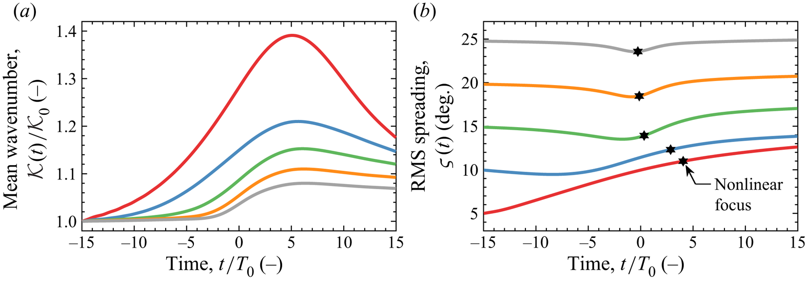
The associated change in mean wavenumber  $\mathcal {K}(t)$ is shown in figure 12(a) for the various cases of directional spreading, normalised by the initial value
 $\mathcal {K}_{0}$. The increase in mean wavenumber is also delayed for cases with more directional spreading due to the comparatively late focusing of the event, but the qualitative trend is consistent. An increase in directional spreading reduces energy transfers and limits the growth in mean wavenumber. However, the change in spreading parameter shown in figure 12(b) depicts a qualitatively different trend for the different cases of directional spreading. Case
 $\varsigma _0=5^{\circ }$ features an increase in directional spreading during focus and ultimately results in a focused event which is more spread than the initial condition – the time of nonlinear focus is indicated with a black hexagram. Case
 $\varsigma _0=10^{\circ }$ features a reduction in directional spreading for a few wave periods after the start of the simulation but thereafter an increase in directional spreading follows and the focused wave event is also more spread than the initial conditions. Conversely, cases
 $\varsigma _0=15^{\circ }$,
 $20^{\circ }$ and
 $25^{\circ }$ feature a reduction in directional spreading before focus and the focused wave event is ultimately less spread than the initial conditions.
Spectral evolution over time for wave groups with a steepness of  $A_{L}k_{p}=0.24$, dimensionless depth of
 $k_{p}d=3.142$ and initial spreading parameters of
 $5^{\circ }$ (thick red),
 $10^{\circ }$ (thick blue),
 $15^{\circ }$ (thick green),
 $20^{\circ }$ (thick orange) and
 $25^{\circ }$ (thick grey). The spectral parameters include: (a) mean wavenumber
 $\mathcal {K}(t)$ normalised by the initial value
 $\mathcal {K}_{0}$; (b) RMS spreading parameter
 $\varsigma (t)$. The time of nonlinear focus is indicated with a black hexagram. All cases are based on a Gaussian wavenumber spectrum with a Gaussian spreading function.

These results suggest that a steep wave event in a sea with low directional spreading, i.e.  $\varsigma _0\leq 10^{\circ }$, may tend to be more spread than the background sea state, while seas with more directional spreading, i.e.
 $\varsigma _0\geq 15^{\circ }$, may produce steep wave events which are less directionally spread than the background sea state. Note, the cases with more directional spreading,
 $\varsigma _0\geq 15^{\circ }$, exhibit a reduction in spreading before focus, but the trend is largely reversed after focus so the final value of the spreading parameter nearly matches the initial value, as demonstrated by case
 $\varsigma _0=25^{\circ }$. However, the cases with low spreading
 $\varsigma _0\leq 10^{\circ }$ do not exhibit such a reversal – the final spreading parameter is significantly larger than the initial spreading parameter.
3.4. Effect of the high-wavenumber tail
The peak of the JONSWAP spectrum contains most of the total energy. Thus, Gaussian wavenumber spectra are frequently used in studies of wave–wave interactions with the high-wavenumber components of the tail neglected from the analysis (see, e.g., Mori, Onorato & Janssen Reference Mori, Onorato and Janssen2011). Certain physical processes have been found to suppress high-wavenumber components, which comprise the tail of the spectrum, more severely than low-wavenumber components. Such mechanisms can suppress the development of the high-wavenumber tail. Wave blocking due to currents (see, e.g., Ma et al. Reference Ma, Dong, Perlin, Ma, Wang and Xu2010) can suppress the tail of the wave spectrum at a particular location, if low-wavenumber components continue to propagate while high-wavenumber components are blocked from propagating further, as discussed by Chawla & Kirby (Reference Chawla and Kirby2002). Rapizo et al. (Reference Rapizo, Waseda, Babanin and Toffoli2016) found that the development of the spectral tail is disturbed for waves propagating on a coflowing current, due to detuning of the quartet resonance interactions. Similarly, Waseda et al. (Reference Waseda, Kinoshita, Cavaleri and Toffoli2015) found that the spectral tail can be suppressed by detuning due to currents. Ice sheets also tend to suppress high-wavenumber components, attenuating the amplitude of high-wavenumber components more severely than low-wavenumber components (see Toffoli et al. Reference Toffoli, Bennetts, Meylan, Cavaliere, Alberello, Elsnab and Monty2015; Meylan et al. Reference Meylan, Bennetts, Mosig, Rogers, Doble and Peter2018), possibly suppressing the tail of the spectrum. Thus, a comparison between Gaussian and JONSWAP spectra serves two purposes: (i) to indicate the appropriacy of a Gaussian spectrum as a model for the peak of a JONSWAP spectrum in typical sea states and; (ii) to contrast the spectral evolution of a steep wave event in seas with and without a fully developed spectral tail.
We combine a JONSWAP wavenumber spectrum ( $\gamma =3.3$) with a frequency-independent spreading function, a Gaussian with an initial spreading parameter of
 $\varsigma _0=15^{\circ }$, and denote this case as JG15. Similarly, we combine a JONSWAP spectrum (
 $\gamma =3.3$) with the frequency-dependent spreading function of Ewans (Reference Ewans1998) and denote this case as JE. The combination of a JONSWAP spectrum with an Ewans (Reference Ewans1998) spreading function realistically captures the spectral shape of fetch-limited seas. We compare against two cases based on a Gaussian wavenumber spectrum: one with an initial spreading parameter of
 $\varsigma _0=15^{\circ }$, denoted as GG15, and another with an initial spreading parameter of
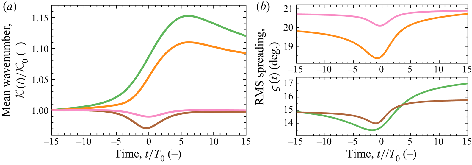
 $\varsigma _0=20^{\circ }$, denoted as GG20. A summary of the case acronyms is listed in table 4. The results are shown in figure 13 for both the mean wavenumber
 $\mathcal {K}(t)$ and spreading parameter
 $\varsigma _0(t)$. The mean wavenumber is normalised by the initial value for each case
 $\mathcal {K}_0$. Figure 13(a) indicates that the simulations performed with a Gaussian wavenumber spectrum produces an increase in mean wavenumber. However, the simulations performed with a JONSWAP spectrum, cases JG15 and JE, exhibit a qualitatively different trend; the mean wavenumber remains approximately constant during the early stages of focusing and reduces during the focus event. Thus, the increase in mean wavenumber observed for the Gaussian cases, GG15 and GG20, appears to be associated with redevelopment of the truncated high-wavenumber tail, and the JONSWAP cases do not show the same trend. The trend for the spreading parameter is, however, qualitatively similar between the Gaussian and JONSWAP cases, as shown in figure 13(b). All cases feature a reduction in the spreading parameter during focus, indicating focused wave events which are less directionally spread than the background sea state, i.e. the ‘wall-of-water’ effect.
The effect of the high-wavenumber tail on the spectral evolution of wave groups with a steepness of  $A_{L}k_{p}=0.24$, dimensionless depth of
 $k_{p}d=3.142$ and different spectral shapes: GG15, thick green; GG20, thick orange; JG15, thick brown; JE, thick pink. The spectral parameters include: (a) mean wavenumber
 $\mathcal {K}(t)$ normalised by the initial value
 $\mathcal {K}_{0}$; (b) RMS spreading parameter
 $\varsigma (t)$ in degrees.

Summary of acronyms for simulation cases.

Thus, a Gaussian wavenumber spectrum exhibits qualitatively similar trends to a JONSWAP spectrum in terms of the spreading parameter, but redevelopment of the spectral tail leads to an increase in mean wavenumber, which is not observed for the JONSWAP spectrum. Furthermore, the changes in mean wavenumber and spreading parameter for the JONSWAP cases appear to be largely temporary since the reduction in both parameters reverses after focus. In contrast, the changes in mean wavenumber and spreading parameter for the Gaussian cases appear to include more permanent changes since the trends do not entirely reverse after focus. Thus, the JONSWAP spectra exhibit a form of spectral equilibrium which inhibits changes to the spectrum. The results of the previous sections based on Gaussian wavenumber spectra may, thus, be most applicable to sea states without a fully developed spectral tail. Energy transfer to higher wavenumbers, in particular, is reduced for steep wave events based on a fully developed JONSWAP spectrum. We conclude that the high-wavenumber tail of the spectrum influences the spectral evolution of a steep wave event. Thus, studies based solely on Gaussian spectra, e.g. Adcock et al. (Reference Adcock, Taylor and Draper2015), should be treated with caution.
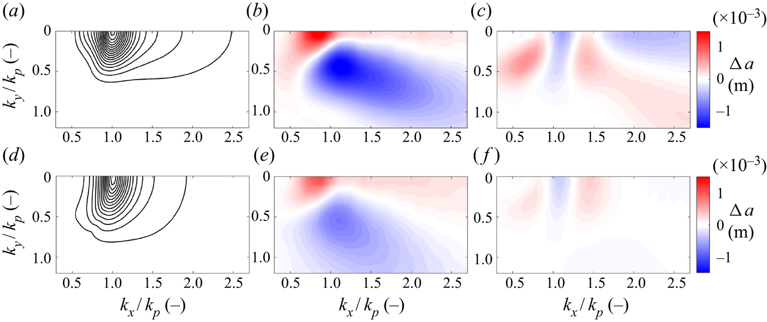
Amplitude spectra of surface elevation, shown in figure 14, depict the spectral evolution of the JONSWAP cases (JG15 and JE). The top row of panels, figure 14(a–c), correspond to case JG15. The bottom row of panels, figure 14(d–f), correspond to case JE. The initial conditions ( $t/T_{0}=-15$) are shown in figure 14(a) and 14(d). The initial conditions indicate that the Ewans (Reference Ewans1998) spreading function of case JE features higher levels of spreading in the tail than the Gaussian spreading function of case JG15. Figure 13(b) confirms that the spreading parameter is consistently lower for case JG15 than case JE, due to lower levels of spreading in the tail for case JG15. The spectral evolution of both JONSWAP cases (JG15 and JE) is less noticeable than the GG cases. Thus, we show the difference in the amplitude spectrum relative to the initial condition: around the time of focus (
 $t/T_{0}=0$) in figure 14(b,e); and at the end of the simulation (
 $t/T_{0}=15$) in figure 14(c,f). We use a colour scale to indicate the growth (in red) and decline (in blue) of component amplitudes relative to the initial condition. As shown in figure 13, the spectral changes are most apparent around the time of focus (
 $t/T_{0}=0$), figure 14(b,e), but the changes appear to be mostly temporary and reverse after focus, leaving few permanent changes at the end of the simulation (
 $t/T_{0}=15$), figure 14(c,f). Case JG15 does exhibit some permanent changes to the spectrum – the directional spreading of the tail increases as energy is transferred to oblique high-wavenumber components, consistent with the net increase in the spreading parameter shown in figure 13(b). In contrast, case JE exhibits fewer permanent changes, consistent with the results of figure 13. Thus, high levels of directional spreading in the tail, e.g. Ewans (Reference Ewans1998), may also be a feature of spectral equilibrium. Case JG15 also exhibits more substantial spectral changes around the time of focus (
 $t/T_{0}=0$), figure 14(b,e). Contraction of the spectrum in the
 $k_y$-direction (the ‘wall-of-water’ effect) and a downshift in the spectral peak occurs for both case JG15 and case JE. However, both effects are more substantial for case JG15, providing further evidence that case JE may be a better representation of spectral equilibrium than case JG15 and directional spreading in the tail can influence spectral evolution.
Amplitude spectra of surface elevation for JONSWAP cases: JG15 in (a,b,c); and JE in (d,e,f). Initial conditions ( $t/T_{0}=-15$) are shown in (a,d) with contour levels (black solid line) evenly distributed between 0.002 and 0.034 m in intervals of 0.002 m. The difference in the amplitude spectrum at time
 $t/T_{0}=0$, relative to the initial condition, is shown in (b,e) using a colour scale with levels shown in the figure. Similarly, the difference in the amplitude spectrum at the end of the simulation (
 $t/T_{0}=15$), relative to the initial condition, is shown in (c,f) using the same colour scale.

3.5. Downshift of the spectral peak
We observe a downshift in wavenumber for the spectral peak during our simulations, see figure 3 as an example. First reported by Lake et al. (Reference Lake, Yuen, Rungaldier and Ferguson1977), the phenomenon is commonly termed a frequency/wavenumber downshift and has been observed by numerous studies (see Ma et al. (Reference Ma, Dong, Perlin, Ma, Wang and Xu2010), Kharif et al. (Reference Kharif, Giovanangeli, Touboul, Grare and Pelinovsky2008a), Segur et al. (Reference Segur, Henderson, Carter, Hammack, Li, Pheiff and Socha2005), Dysthe et al. (Reference Dysthe, Trulsen, Krogstad and Socquet-Juglard2003), Melville (Reference Melville1982), Su et al. (Reference Su, Bergin, Marler and Myrick1982) and others). Downshifting has been related to nonlinear wave–wave interactions (e.g. Trulsen & Dysthe Reference Trulsen and Dysthe1997), breaking (e.g. Trulsen & Dysthe Reference Trulsen, Dysthe, Tørum and Gudmestad1990; Tulin & Waseda Reference Tulin and Waseda1999) and wind (e.g. Hara & Mei Reference Hara and Mei1991). The downshift we observe in our potential flow simulations is exclusively due to nonlinear wave–wave interactions. We base our analysis on component  $\mathcal {Q}$ (
 $k_{x}/k_{p}=1.000$,
 $k_{y}/k_{p}=0.000$), which coincides initially with the peak of the wavenumber spectrum. The rate of change in wave action density for
 $\mathcal {Q}$ is indicative of the rate of downshift for the spectral peak, and we consider the influences of directional spreading and the high-wavenumber tail on the downshift, with the results shown in figure 15. We consider Gaussian wavenumber spectra with a Gaussian spreading function and initial spreading parameters (
 $\varsigma _{0}$) of
 $5^{\circ }$,
 $10^{\circ }$,
 $15^{\circ }$,
 $20^{\circ }$,
 $25^{\circ }$; the cases are denoted as GG5, GG10, GG15, GG20 and GG25, respectively. For comparison, we consider a JONSWAP spectrum (
 $\gamma =3.3$) with frequency-independent spreading, based on a Gaussian spreading function with
 $\varsigma _{0}=15^{\circ }$, and denote this case as JG15. We also consider a JONSWAP spectrum with frequency-dependent spreading, based on the Ewans (Reference Ewans1998) spreading function, and denote this case as JE. A linear steepness at focus (
 $A_{L}k_{p}$) of 0.24 has been selected for all cases together with a depth (
 $k_{p}d$) of 3.142.
Growth rate of wave action density  $\mathcal {A}$ for the spectral component
 $\mathcal {Q}$, which initially coincides with the peak of the amplitude spectrum: (a) GG5; (b) GG10; (c) GG15; (d) GG20; (e) GG25; (f) JG15; (g) JE. The dynamic growth rate
 $O(\epsilon ^{2}\omega _{0}T_{0})$ is indicated by bounded (bold dashed line) grey bands. The magenta line segment (thick magenta) indicates the time interval during which
 $A(t)k_{p}$, as shown in figure 11, exceeds 0.18. The value of
 $\epsilon$ equates to
 $A_{L}k_{p}/{\rm \pi}$ in the calculation of the growth rates. The time of nonlinear focus is indicated with a hexagram.

The growth rate for component  $\mathcal {Q}$ is shown in figure 15 for the various cases together with the dynamic time scale. For all cases except GG5, the wave action of component
 $\mathcal {Q}$ initially increases before the downshift of the peak begins (see figure 4a as an example). The growth rate is shown in absolute terms. Thus, a discontinuity is shown in the logarithmic plots, at the time of maximum wave action density, when the growth rate momentarily reaches zero before a change in sign occurs. The time of nonlinear focus for each case is indicated with a black hexagram in figure 15, and the time interval for which the steepness of the wave envelope
 $A(t)k_{p}$ exceeds 0.18 is indicated by a magenta line segment. The growth rate for case GG5 is augmented because the steepness of the event exceeds the linear steepness, used to calculate the dynamic growth rate, as evidenced by figure 11(a). The other GG cases achieve a steepness at focus which is comparable to the linear steepness, and the post-focus growth rate for component
 $\mathcal {Q}$ can be seen in figure 15 to be consistent with the dynamic time scale. However, an increase in directional spreading for the GG cases does reduce the rate of downshift for the spectral peak and the inclusion of the high-wavenumber tail of the spectrum, featured in the JG15 and JE cases, leads to a further decrease.
The effect of the high-wavenumber tail on the downshift is summarised in figure 16, which shows the maximum growth rate, at any time in the simulation, on the vertical axis. The horizontal axis shows the corresponding spreading parameter ( $\varsigma (t)$), at the time that the maximum growth rate occurs. Cases GG15 and JG15 exemplify the role of the high-wavenumber tail in reducing the downshift phenomenon; the two cases exhibit a similar spreading parameter but the maximum growth rate for case GG15 is a factor of three faster than case JG15. The slower growth rate for case JG15 is particularly noteworthy because the JG15 focused wave event is arguably steeper than the GG15 event. The linear steepness is calculated from
 $A_{L}k_{p}$, which incorporates the spectral peak, at the start of the simulation, as the characteristic wavenumber. A Gaussian wavenumber spectrum is symmetric about the spectral peak which supports the use of
 $k_{p}$ as the characteristic wavenumber, particularly if the spectrum is narrow-banded. However, a JONSWAP spectrum features a high-wavenumber tail which arguably should result in a characteristic wavenumber above
 $k_{p}$, suggesting cases JG15 and JE are steeper than indicated by
 $A_{L}k_{p}$. However, the maximum growth rate for case GG15 is significantly higher than the maximum growth rate for cases JG15 and JE. Inclusion of the high-wavenumber tail, thus, appears to reduce the downshift of the spectral peak.
The stabilising effect of directional spreading and the high-wavenumber tail: the vertical axis indicates the maximum growth rate calculated at any point in the simulation; the horizontal axis indicates the RMS spreading parameter of the spectrum at the corresponding time. The growth rate calculation is based on component  $\mathcal {Q}$ (
 $k_{x}/k_{p}=0.995$,
 $k_{y}/k_{p}=0.000$), which initially coincides with the peak of the wavenumber spectrum. The various cases, all with a steepness of
 $A_{L}k_{p}=0.24$ and a depth of
 $k_{p}d=3.142$, are labelled within the figure. The dynamic growth rate
 $O(\epsilon ^{2}\omega _{0}T_{0})$ is indicated by bounded (bold dashed line) grey bands. The value of
 $\epsilon$ equates to
 $A_{L}k_{p}/{\rm \pi}$ in the growth rate calculations.

In summary, all focused wave events in this study exhibit a downshift of the spectral peak. However, spreading and the inclusion of the high-wavenumber tail reduce the downshift, and nonlinear evolution of the wavenumber spectrum in general. The mechanism is not limited to a reduced focal time caused by linear dispersion. Rather, the rate of the downshift, even at the steepest stages of focusing, is also reduced by spreading and the high-wavenumber tail. Thus, directional spreading and the spectral tail appear to be integral features of a spectral equilibrium, which limits directional energy transfers during a steep wave event.
4. Conclusion
We have studied steep focusing wave groups formed by dispersive focusing in deep and intermediate waters. For narrow-banded Gaussian wavenumber spectra with a Gaussian spreading function, quasi-degenerate interactions result in directional energy transfers: (i) along the  $k_x$-axis, consistent with the unidirectional instabilities observed by Longuet-Higgins (Reference Longuet-Higgins1978) and McLean (Reference McLean1982b) for a regular wave; (ii) at angles of
 ${\pm }35^{\circ }$ to the spectral peak with a bias towards high-wavenumber components, consistent with the
 $\arctan {(1/\sqrt {2})}$ resonance angle identified by Longuet-Higgins (Reference Longuet-Higgins1976) and the Phillips ‘figure-of-eight’ resonance loop.
Spectral broadening due to the quasi-degenerate interactions eventually facilitates non-degenerate interactions, which dominate the spectral evolution of the wave group after focus. The non-degenerate interactions manifest as high-wavenumber sidelobes at angles of  ${\pm }55^{\circ }$ to the spectral peak. We also observe contraction of the wavenumber spectrum in the
 $k_{y}$-direction during focusing and a downshift in wavenumber for the spectral peak, consistent with previous studies (see, e.g., Trulsen & Dysthe Reference Trulsen and Dysthe1997). All the spectral changes we observe can be attributed to quartet interactions. Relative to linear theory, the combination of quasi-degenerate and non-degenerate interactions results in nonlinear wave events with augmented kinematics and an extended lifespan.
Finite depth weakens all forms of spectral evolution. However, the quasi-degenerate interactions exhibit a greater sensitivity to depth, indicating suppression of the modulation instability by the return current as discussed by Dysthe (Reference Dysthe1979) and Janssen & Onorato (Reference Janssen and Onorato2007). We also observe sensitivity to depth for  $k_{p}d$ values commonly considered to be deep,
 $3.142<k_{p}d<5.592$. The non-degenerate interactions appear to be significantly less suppressed by depth with persistent evidence of a
 ${\pm }55^{\circ }$ spectral sidelobe at a depth of
 $k_{p}d=1.363$. Although the quasi-degenerate interactions are significantly suppressed by depth, the interactions do not entirely disappear for
 $k_{p}d=1.363$ and show signs of biasing towards oblique rather than unidirectional wave components at intermediate depths, consistent with McLean (Reference McLean1982a). The contraction of the wavenumber spectrum in the
 $k_{y}$-direction has also proved to be resilient to depth, suggesting that lateral expansion of the wave group and the ‘wall-of-water’ effect may persist at intermediate depths.
We contrast our analyses of Gaussian cases with simulations based on a JONSWAP spectrum, combined with frequency-independent and frequency-dependent spreading, and find that the high-wavenumber tail of the spectrum reduces the nonlinear features observed for the Gaussian cases. In particular, the energy transfers to higher wavenumbers is reduced for the JONSWAP cases, suggesting that the Gaussian simulations are influenced by the absence of a spectral tail and the nonlinear interactions bias towards redevelopment of the tail. However, the trends in the spreading parameter show qualitative agreement between the Gaussian and JONSWAP cases. We conclude that focused wave events in sea states without a fully developed spectral tail are more likely to exhibit rapid nonlinear evolution. Physical mechanisms which can suppress the high-wavenumber components in the spectral tail, such as dissipation by ice sheets (see Meylan et al. Reference Meylan, Bennetts, Mosig, Rogers, Doble and Peter2018) and wave blocking by currents (see Chawla & Kirby Reference Chawla and Kirby2002), could thus influence the characteristics of focused wave events in the immediate vicinity. We also consider the downshift of the spectral peak and find that the downshift, and the spectral evolution in general, is reduced by directional spreading and the presence of the high-wavenumber tail. Reduced spectral evolution is not only due to the reduced focal time of the more broad-banded events. Rather, the rates of energy transfer also appear to be reduced even at the steepest stages of wave group focusing. Thus, directional spreading and the high wavenumber tail appear to be integral features of a spectral equilibrium which reduces the rapid directional energy transfers of a steep wave group.
Acknowledgements
The authors gratefully acknowledge funding from the DeRisk project of Innovation Fund Denmark (grant number 4106-00038B). T.S.v.d.B. acknowledges a Royal Academy of Engineering Research Fellowship. D.B. has been supported by a studentship from the Engineering and Physical Sciences Research Council (EPSRC) of the UK Government and would like to specifically thank P. S. Tromans of Ocean Wave Engineering Ltd. as well as A. V. Babanin and Q. Liu of the University of Melbourne for useful discussions about this work.
Declaration of interests
The authors report no conflict of interest.