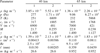
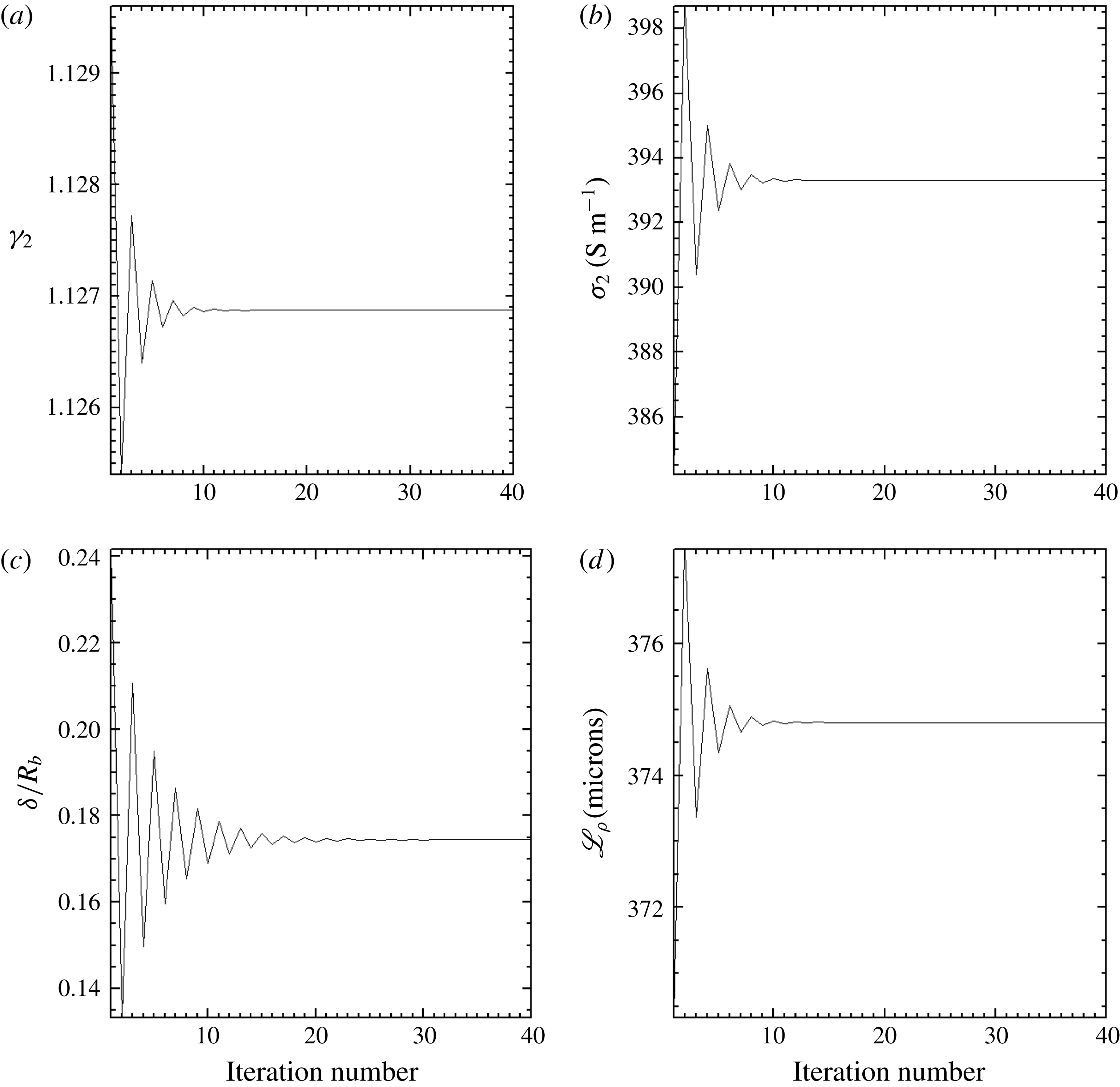
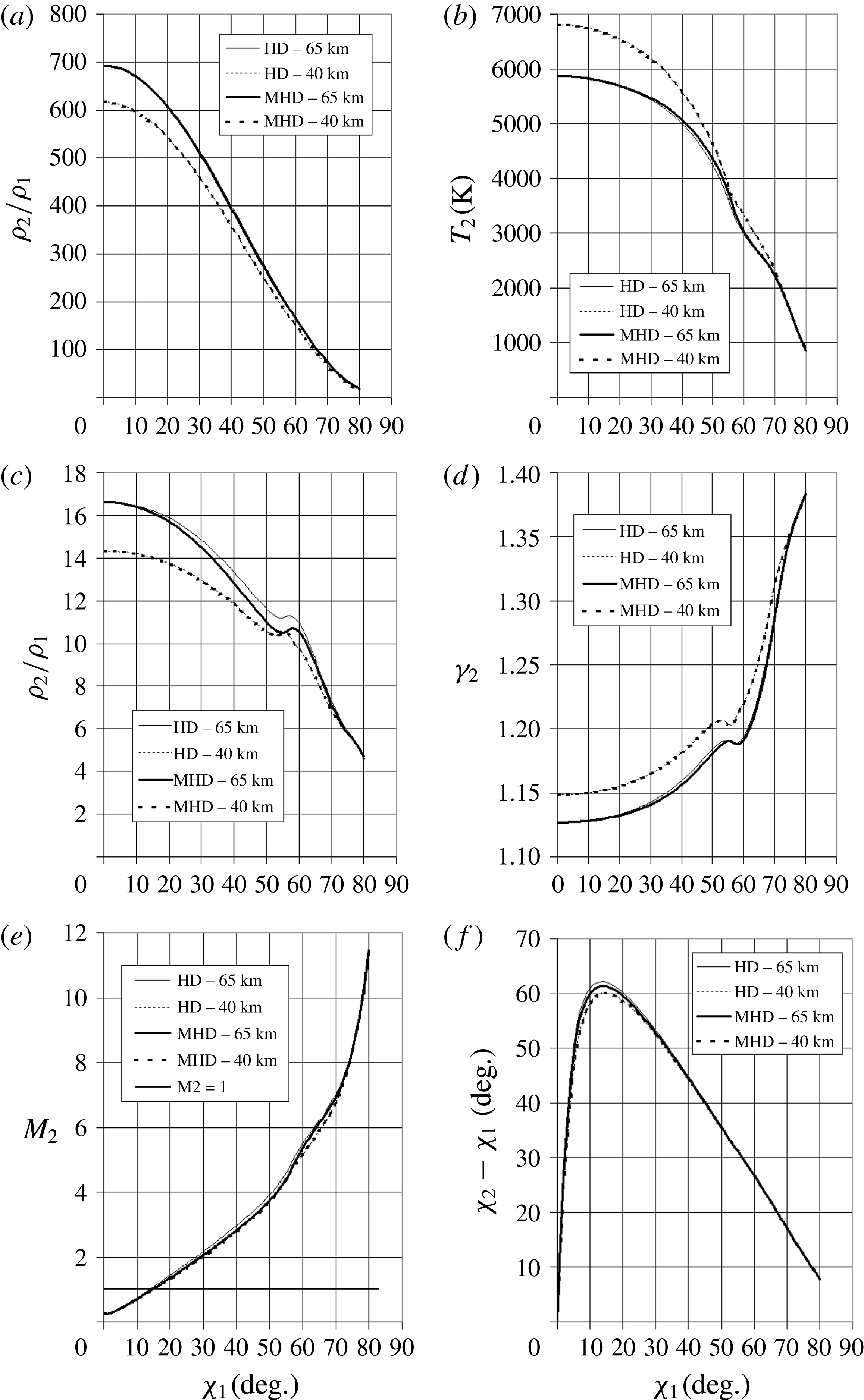
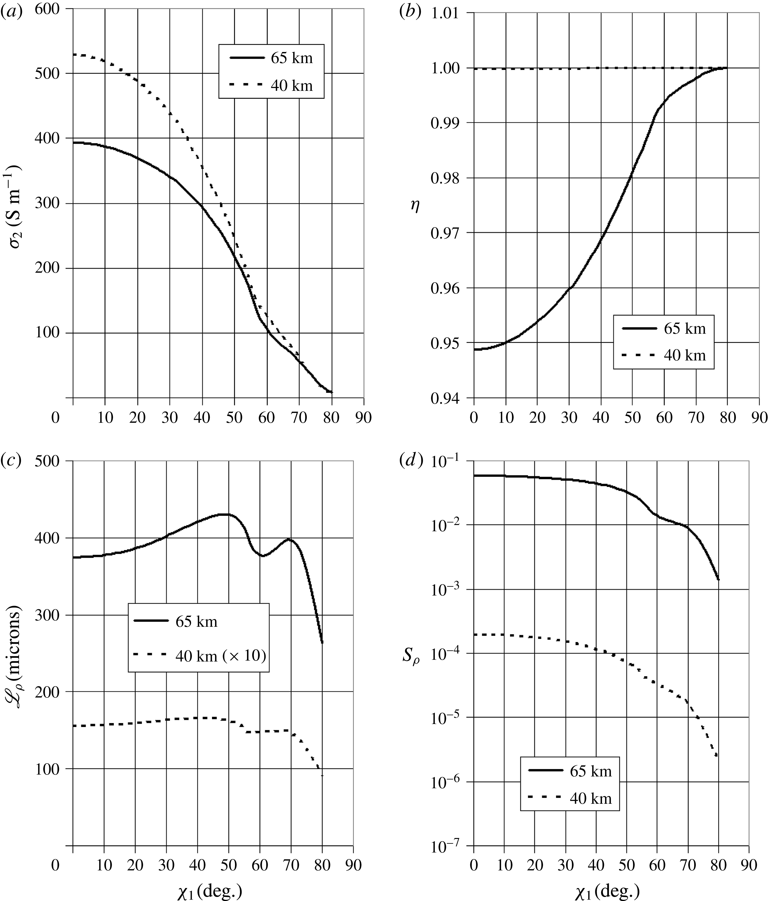
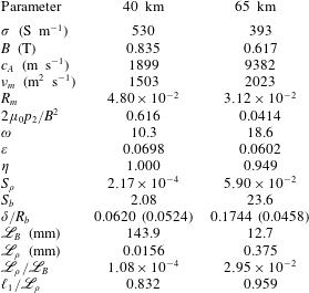
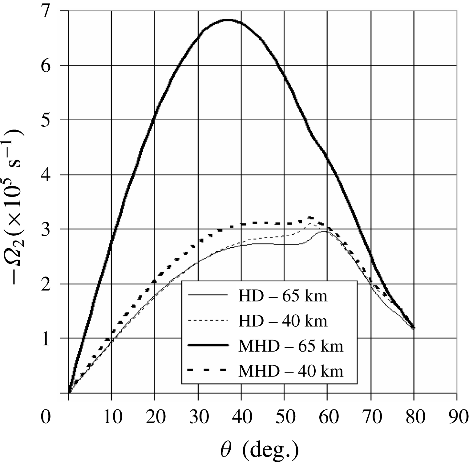
1 Introduction
The magnetohydrodynamic (MHD) interaction of an ionized flow with a magnetized body moving in the atmosphere at a hypersonic speed was modelled as early as the 1950s, initiated with theoretical approaches (Bush Reference Bush1958; Levy Reference Levy1963; Levy & Petschek Reference Levy and Petschek1963; Jarvinen Reference Jarvinen1965) and afterwards complemented by numerical simulations stimulated by space flight and atmospheric entry problems (signal blackout, wall heating, drag monitoring,
 $\ldots$
). Numerical resolution of the Euler equations for the aerodynamic blunt-body problem at supersonic speeds was developed in the 1960s (Moretti & Abbett Reference Moretti and Abbett1966; Moretti & Bleich Reference Moretti and Bleich1967; Rusanov Reference Rusanov1976), soon followed by numerical resolution of the MHD equations (Coackley & Porter Reference Coackley and Porter1971), and has reached a high level of accuracy.
Nevertheless, analytical tools presently in development have renewed the understanding of phenomena and proved the necessity of a complementary approach to cope with nonlinear problems (Maicke, Barber & Majdalani Reference Maicke, Barber and Majdalani2010). Moreover, system models require the instantaneous calculation of forces and heat fluxes along trajectories. Therefore, the analytic approach of the present paper, extending the classical Rankine–Hugoniot relations (Rankine Reference Rankine1870; Hugoniot Reference Hugoniot1889), opens a prospect towards MHD shock fitting as an alternative to the shock-capturing approach broadly used in the many numerical models published and in progress. The respective advantages and drawbacks of shock fitting over shock capturing have been recently pointed out in aerodynamic applications (Moretti Reference Moretti2002; Bonfiglioli & Paciorri Reference Bonfiglioli and Paciorri2010; Pepe et al. Reference Pepe, Bonfiglioli, D’Angola, Colonna and Paciorri2014).
In ideal MHD problems, frequently solved in various media, it is assumed that the electrical conductivity of the flowing medium is infinite – or, more accurately, the magnetic Reynolds number is infinite. This greatly simplifies the equations and, in solar physics for instance, enables one to eliminate the electric field. Owing to the large volumes involved, the magnetic Reynolds number is actually very large (
 ${\sim}10^{5}$
) and causes the magnetic field to evolve, producing dynamo effects, for instance in solar active regions (Priest Reference Priest1987, chap. 5; Berton Reference Berton2000).
In the present case of re-entry MHD problems, the conductivity is also finite, but the small volumes involved do not allow one to eliminate the electric field and let an applied magnetic field persist, since the magnetic Reynolds number is very small (
 ${\sim}10^{-3}$
), so that the steady state can therefore be considered as a first approach. Moreover, symmetry considerations lead one to set the electrostatic field to zero. We shall assume a finite conductivity and derive in the next section the original jump equations.
First, an oblique MHD shock with real gas effects due to air dissociation will be considered. In this first task, viscous and thermal effects, as well as the Hall effect arising when the electric conductivity becomes a tensor (at altitudes above 50 km), have been neglected (Levy Reference Levy1963; Ericson & Maciulaitis Reference Ericson and Maciulaitis1964). The expressions thus obtained are compared with the existing hydrodynamic Rankine–Hugoniot formulae, which are also usually derived without viscous and thermal effects but also without jump of the isentropic exponent. As will be shown, the jump expressions depend not only on the usual hydrodynamic ratio
 $\unicode[STIX]{x1D700}$
of mass densities, but also on a new MHD parameter, denoted
 $\unicode[STIX]{x1D702}$
, acting as a bending parameter of streamlines. Because of the ionizing action of the shock, the electric conductivity is assumed to be zero ahead of the shock.
In § 3, test cases are examined in order to check the jump equations for a plane shock in simple configurations. For this purpose, we make use of existing thermodynamic models of dissociated air and work out a shock-fitting method with the isentropic exponent. The problems arising from the assumptions are put into evidence, in parallel with aerodynamic situations. An important similarity rule is put into evidence and is confirmed in § 5.
In § 4, as an application, we describe the procedure of a detached spherical shock fitting, and for this purpose make use of the same models of dissociated air and a model of conductivity. The fitting procedure is extended to other parameters (conductivity, shock distance and thickness). The MHD results are compared with hydrodynamic solutions for the physical conditions at two altitudes along a re-entry trajectory.
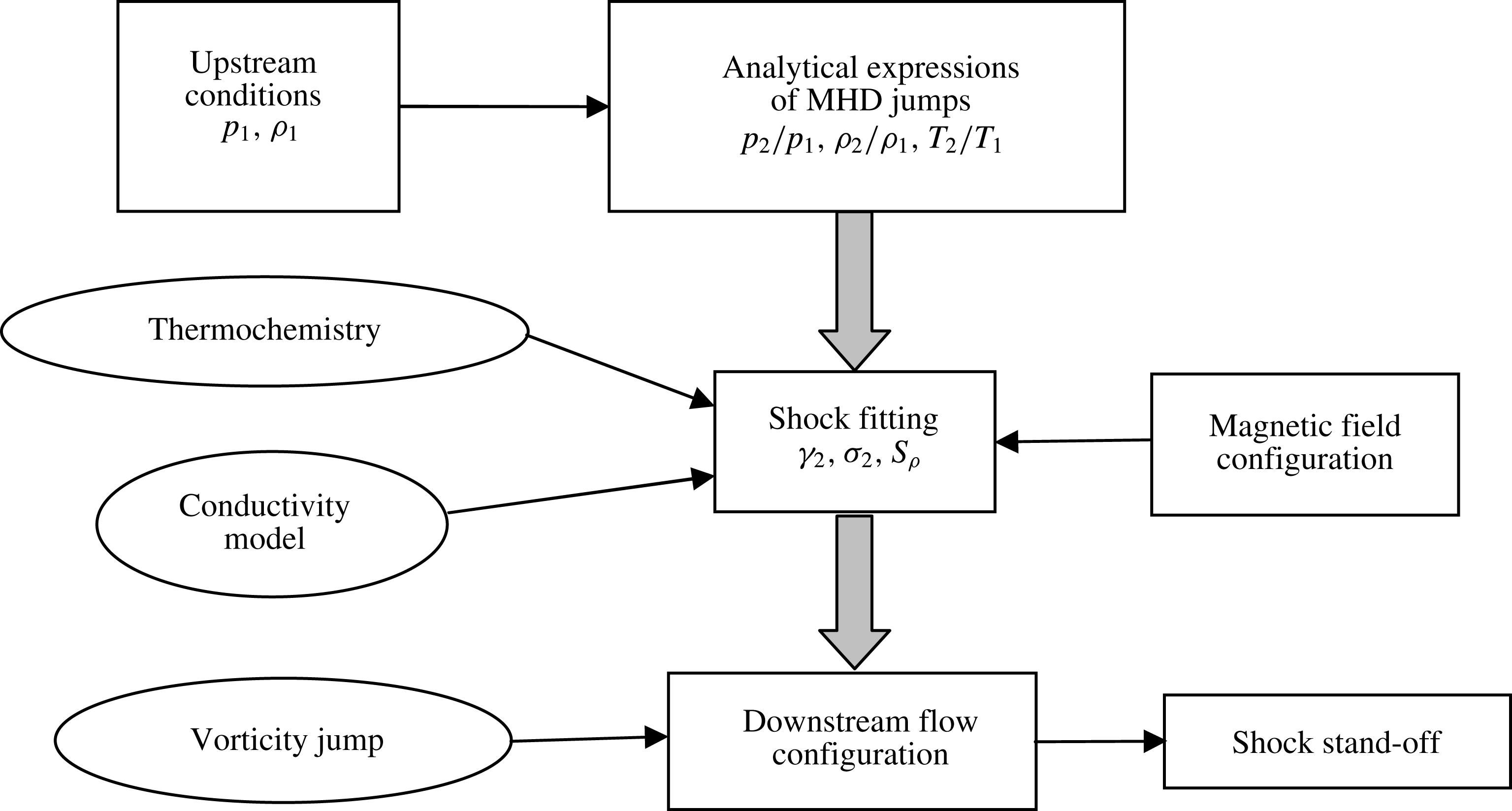
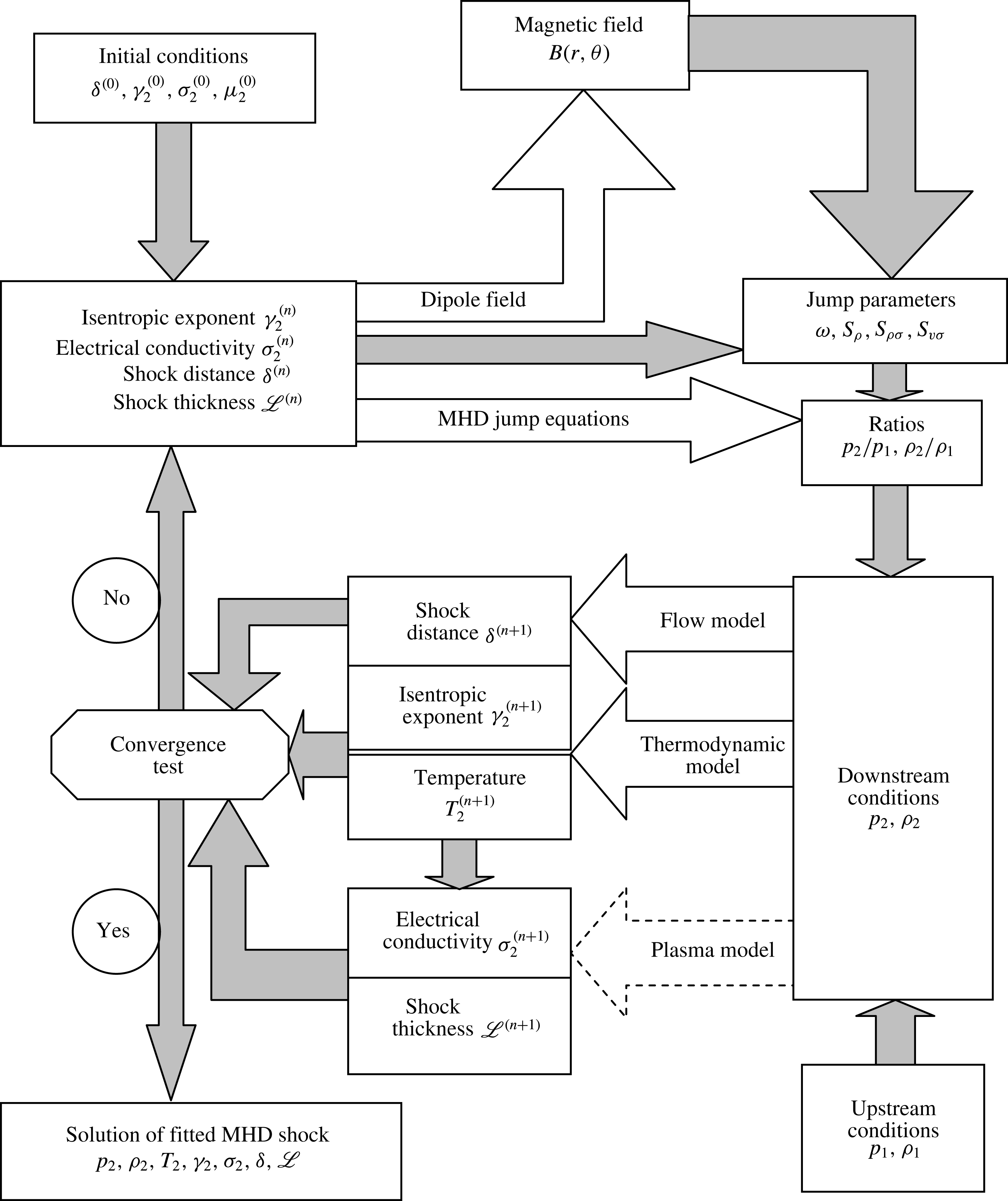
Flowchart of the proposed analytic approach for an MHD resistive shock.

In § 5, a simplified model of the flow behind the shock produced by a blunt body is proposed on the basis of stream functions matched with the corresponding one ahead of the shock and taking into account MHD and real gas effects. We consider a rotational flow taking into account a vorticity jump at the shock. Shock stand-off is estimated and compared with existing models. The overall approach is depicted in figure 1.
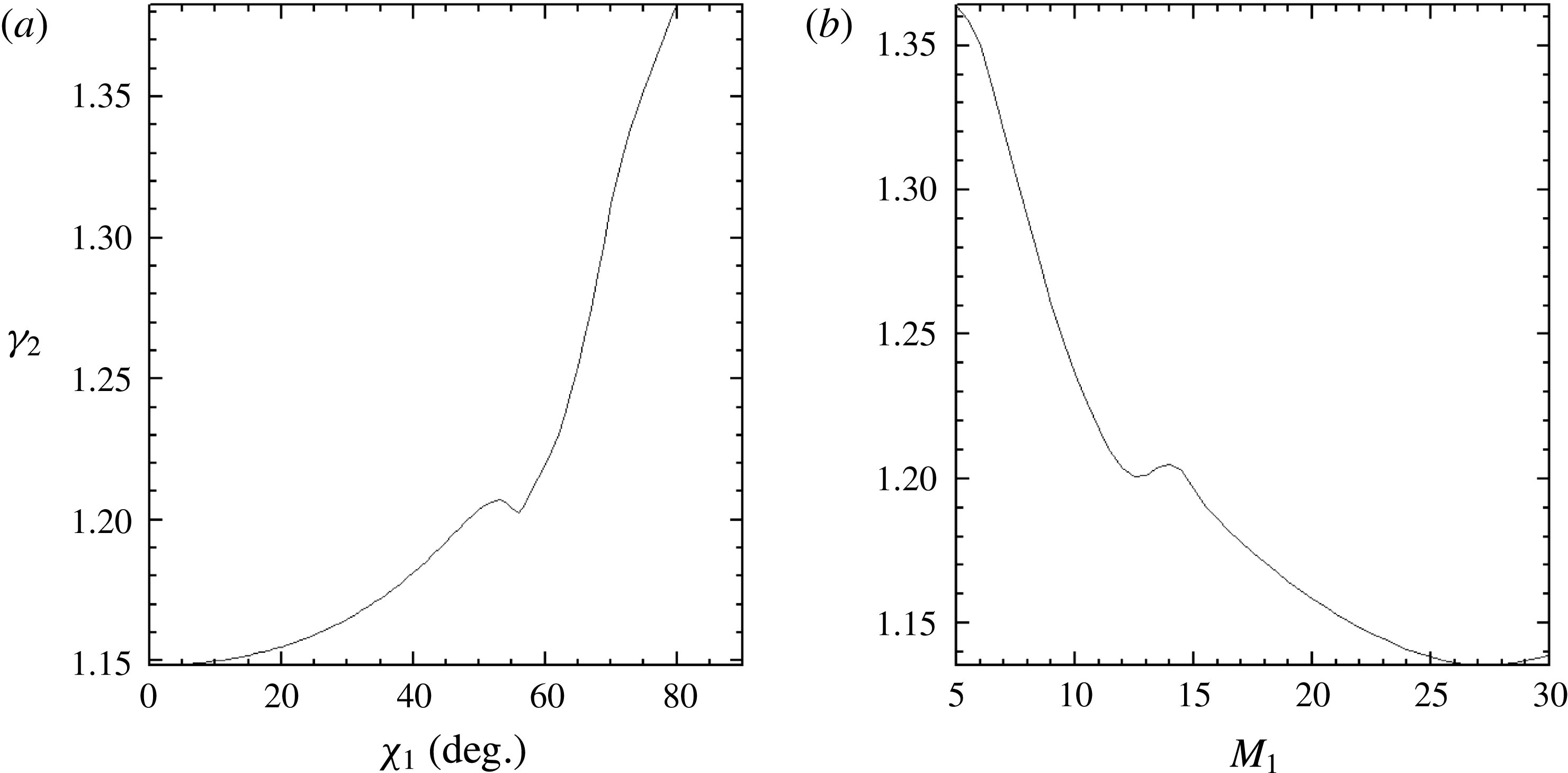
The similarity rule put into evidence in § 3, involving the hypersonic parameter
 $M_{1}\cos \unicode[STIX]{x1D712}_{1}$
, shows a correspondence between the upstream Mach number
 $M_{1}$
and the velocity angle
 $\unicode[STIX]{x1D712}_{1}$
. The model of shock thickness used appears to be limited to
 $\unicode[STIX]{x1D712}_{1}<50^{\circ }$
.
In § 6, an assessment of the re-entry application is proposed. Magnetohydrodynamic effects inside the shock are compared with MHD effects in the shock layer.
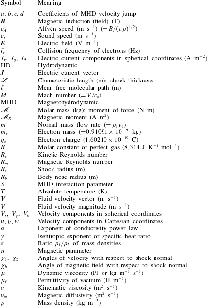
Conclusions and prospects for trajectories in re-entry problems are discussed in the final section. The validity of our approximations is examined, and justifications and remedies are proposed. Notations used throughout the paper are defined in table 1.
Nomenclature of symbols and notations.

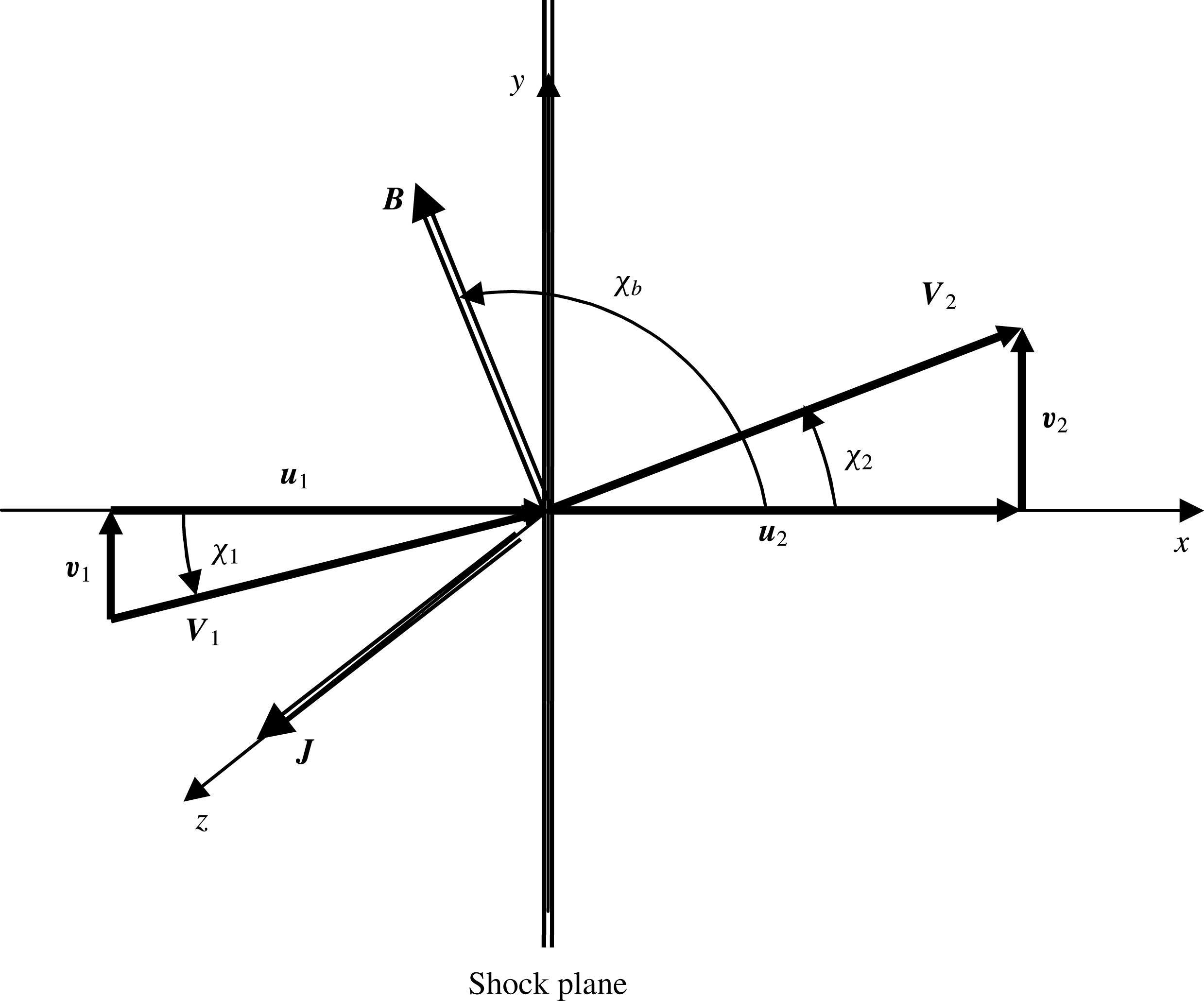
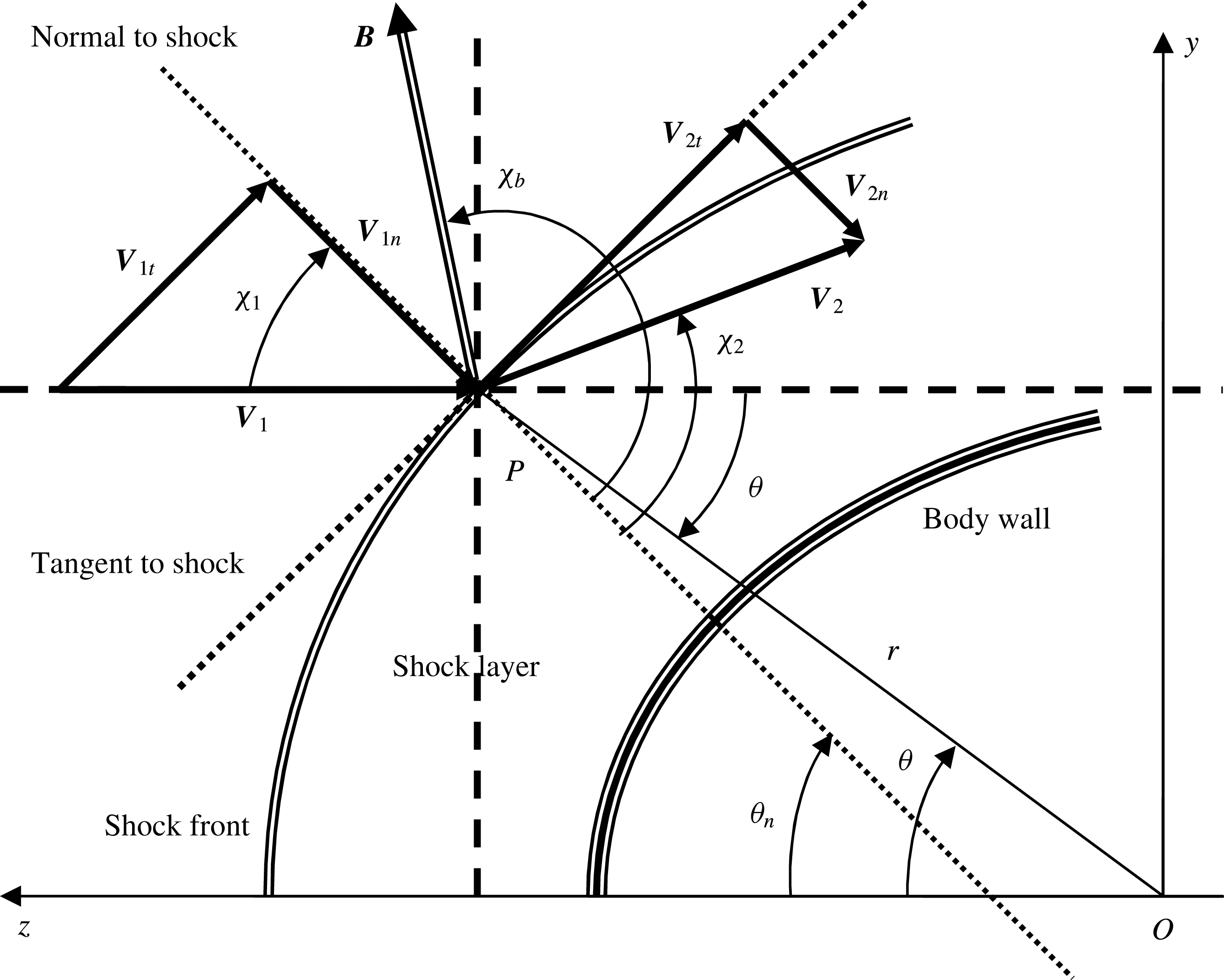
Geometrical configuration of a plane oblique MHD shock. The current vector
 $\boldsymbol{J}$
along
 $z$
is perpendicular to the
 $x$
–
 $y$
plane and lies in the shock plane.

2 Resistive MHD jump conditions
2.1 Basic equations
Let us consider a stationary plane oblique shock in a flow moving from left to right (figure 2). In the following sections, subscripts 1 and 2 respectively denote quantities ahead of the shock (upstream) and behind it (downstream). In hydrodynamics, the classical Rankine–Hugoniot relations giving the pressure and density ratios through such a shock are well known and are written respectively for a perfect gas with a constant isentropic exponent
 $\unicode[STIX]{x1D6FE}$
(Hugoniot Reference Hugoniot1889) as
 $$\begin{eqnarray}\displaystyle \displaystyle \frac{p_{2}}{p_{1}}=\frac{2\unicode[STIX]{x1D6FE}M_{1}^{2}\cos ^{2}\unicode[STIX]{x1D712}_{1}-(\unicode[STIX]{x1D6FE}-1)}{\unicode[STIX]{x1D6FE}+1},\quad \frac{\unicode[STIX]{x1D70C}_{2}}{\unicode[STIX]{x1D70C}_{1}}=\frac{(\unicode[STIX]{x1D6FE}+1)M_{1}^{2}\cos ^{2}\unicode[STIX]{x1D712}_{1}}{(\unicode[STIX]{x1D6FE}-1)M_{1}^{2}\cos ^{2}\unicode[STIX]{x1D712}_{1}+2}. & & \displaystyle\end{eqnarray}$$
The normal shock is retrieved when
 $\unicode[STIX]{x1D712}_{1}=0$
. The hypersonic hydrodynamic shock relations are obtained as
 $M_{1}\rightarrow +\infty$
,
 $$\begin{eqnarray}\displaystyle \displaystyle \frac{p_{2}}{p_{1}}\approx \frac{2\unicode[STIX]{x1D6FE}M_{1}^{2}\cos ^{2}\unicode[STIX]{x1D712}_{1}}{\unicode[STIX]{x1D6FE}+1},\quad \frac{\unicode[STIX]{x1D70C}_{2}}{\unicode[STIX]{x1D70C}_{1}}=\frac{\unicode[STIX]{x1D6FE}+1}{\unicode[STIX]{x1D6FE}-1}. & & \displaystyle\end{eqnarray}$$
The angle
 $\unicode[STIX]{x1D712}_{2}$
of the downstream velocity satisfies the equation
 $$\begin{eqnarray}\displaystyle \displaystyle \tan \unicode[STIX]{x1D712}_{2}=\frac{\unicode[STIX]{x1D70C}_{2}}{\unicode[STIX]{x1D70C}_{1}}\tan \unicode[STIX]{x1D712}_{1}. & & \displaystyle\end{eqnarray}$$
It is important to notice that for a physically acceptable shock, we must have
 $p_{2}/p_{1}>0$
, and this implies that
 $\unicode[STIX]{x1D712}_{1}$
must be smaller than a critical angle
 $\unicode[STIX]{x1D712}_{1c}$
solution of the equation
 $$\begin{eqnarray}\displaystyle \displaystyle \cos \unicode[STIX]{x1D712}_{1c}=\frac{1}{M_{1}}\sqrt{\frac{\unicode[STIX]{x1D6FE}-1}{2\unicode[STIX]{x1D6FE}}}. & & \displaystyle\end{eqnarray}$$
For a perfect gas with
 $\unicode[STIX]{x1D6FE}=1.4$
and at a hypersonic speed
 $M_{1}=20$
, this gives a critical angle
 $\unicode[STIX]{x1D712}_{1c}=88.9^{\circ }$
.
In order to derive the resistive MHD jump conditions, let us write, in the frame of the moving body (and ambient air at rest), the partial differential equations expressing on one hand the conservation of mass, momentum and energy (Sutton & Sherman Reference Sutton and Sherman2006),
 $$\begin{eqnarray}\displaystyle \left.\begin{array}{@{}l@{}}\displaystyle \frac{\unicode[STIX]{x2202}}{\unicode[STIX]{x2202}x}(\unicode[STIX]{x1D70C}u)+\frac{\unicode[STIX]{x2202}}{\unicode[STIX]{x2202}y}(\unicode[STIX]{x1D70C}v)=0,\\[18.0pt] \displaystyle \unicode[STIX]{x1D70C}u\frac{\unicode[STIX]{x2202}u}{\unicode[STIX]{x2202}x}=-\frac{\unicode[STIX]{x2202}p}{\unicode[STIX]{x2202}x}+\frac{\unicode[STIX]{x2202}}{\unicode[STIX]{x2202}x}\left(\frac{4}{3}\unicode[STIX]{x1D707}\frac{\unicode[STIX]{x2202}u}{\unicode[STIX]{x2202}x}\right)-\unicode[STIX]{x1D70E}(E+uB\sin \unicode[STIX]{x1D712}_{b}-vB\cos \unicode[STIX]{x1D712}_{b})B\sin \unicode[STIX]{x1D712}_{b},\\[18.0pt] \displaystyle \unicode[STIX]{x1D70C}u\frac{\unicode[STIX]{x2202}v}{\unicode[STIX]{x2202}x}=-\frac{\unicode[STIX]{x2202}p}{\unicode[STIX]{x2202}y}+\frac{\unicode[STIX]{x2202}}{\unicode[STIX]{x2202}x}\left(\frac{4}{3}\unicode[STIX]{x1D707}\frac{\unicode[STIX]{x2202}v}{\unicode[STIX]{x2202}x}\right)+\unicode[STIX]{x1D70E}(E+uB\sin \unicode[STIX]{x1D712}_{b}-vB\cos \unicode[STIX]{x1D712}_{b})B\cos \unicode[STIX]{x1D712}_{b},\\[18.0pt] \displaystyle \unicode[STIX]{x1D70C}u\frac{\unicode[STIX]{x2202}}{\unicode[STIX]{x2202}x}\left(h+{\displaystyle \frac{u^{2}+v^{2}}{2}}\right)=\frac{\unicode[STIX]{x2202}}{\unicode[STIX]{x2202}x}\left(\frac{4}{3}\unicode[STIX]{x1D707}u\frac{\unicode[STIX]{x2202}u}{\unicode[STIX]{x2202}x}+\frac{4}{3}\unicode[STIX]{x1D707}v\frac{\unicode[STIX]{x2202}v}{\unicode[STIX]{x2202}x}\right)\\[18.0pt] +\,\unicode[STIX]{x1D70E}(E+uB\sin \unicode[STIX]{x1D712}_{b}-vB\cos \unicode[STIX]{x1D712}_{b})E,\end{array}\right\} & & \displaystyle\end{eqnarray}$$
and on the other hand Maxwell’s equations, (Sutton & Sherman Reference Sutton and Sherman2006)
 $$\begin{eqnarray}\displaystyle \left.\begin{array}{@{}c@{}}\displaystyle \frac{\unicode[STIX]{x2202}}{\unicode[STIX]{x2202}x}\left(B\cos \unicode[STIX]{x1D712}_{b}\right)+\frac{\unicode[STIX]{x2202}}{\unicode[STIX]{x2202}y}\left(B\sin \unicode[STIX]{x1D712}_{b}\right)=0,\\[12.0pt] \displaystyle \frac{\unicode[STIX]{x2202}}{\unicode[STIX]{x2202}x}\left(B\sin \unicode[STIX]{x1D712}_{b}\right)-\frac{\unicode[STIX]{x2202}}{\unicode[STIX]{x2202}y}\left(B\cos \unicode[STIX]{x1D712}_{b}\right)=0,\\[12.0pt] \displaystyle \frac{\unicode[STIX]{x2202}}{\unicode[STIX]{x2202}z}\left(B\sin \unicode[STIX]{x1D712}_{b}\right)=0,\\[12.0pt] \displaystyle \frac{\unicode[STIX]{x2202}}{\unicode[STIX]{x2202}z}\left(B\cos \unicode[STIX]{x1D712}_{b}\right)=0,\end{array}\right\} & & \displaystyle\end{eqnarray}$$
with
 $$\begin{eqnarray}\displaystyle \displaystyle E=-\frac{\unicode[STIX]{x2202}\unicode[STIX]{x1D719}}{\unicode[STIX]{x2202}z},\quad J=\unicode[STIX]{x1D70E}(E+uB\sin \unicode[STIX]{x1D712}_{b}-vB\cos \unicode[STIX]{x1D712}_{b}),\quad h=\frac{\unicode[STIX]{x1D6FE}}{\unicode[STIX]{x1D6FE}-1}\frac{p}{\unicode[STIX]{x1D70C}}. & & \displaystyle\end{eqnarray}$$
The vectors
 $\boldsymbol{V}$
and
 $\boldsymbol{B}$
define the figure plane, and
 $u$
,
 $v$
denote velocity components along axes
 $x$
and
 $y$
, respectively normal and tangent to the shock. The vectors
 $\boldsymbol{E}$
and
 $\boldsymbol{J}$
are perpendicular to this plane. The relation defining the electric current
 $J$
in (2.7) expresses Ohm’s law. Notations are otherwise defined in the nomenclature (table 1).
The property of invariance assumed along
 $y$
and
 $z$
implies that
 $$\begin{eqnarray}\displaystyle \displaystyle E=0,\quad J=\unicode[STIX]{x1D70E}(uB\sin \unicode[STIX]{x1D712}_{b}-vB\cos \unicode[STIX]{x1D712}_{b}),\quad \frac{\unicode[STIX]{x2202}B}{\unicode[STIX]{x2202}z}=0,\quad \frac{\unicode[STIX]{x2202}\unicode[STIX]{x1D712}_{b}}{\unicode[STIX]{x2202}z}=0. & & \displaystyle\end{eqnarray}$$
This leads to recasting system (2.5) into the following system of ordinary differential equations:
 $$\begin{eqnarray}\displaystyle \left.\begin{array}{@{}c@{}}\displaystyle \frac{\text{d}}{\text{d}x}(\unicode[STIX]{x1D70C}u)=0,\\[12.0pt] \displaystyle \unicode[STIX]{x1D70C}u\frac{\text{d}u}{\text{d}x}=-\displaystyle \frac{\text{d}p}{\text{d}x}+\frac{\text{d}}{\text{d}x}\left(\frac{4}{3}\unicode[STIX]{x1D707}\frac{\text{d}u}{\text{d}x}\right)-\unicode[STIX]{x1D70E}B^{2}(u\sin \unicode[STIX]{x1D712}_{b}-v\cos \unicode[STIX]{x1D712}_{b})\sin \unicode[STIX]{x1D712}_{b},\\[12.0pt] \displaystyle \unicode[STIX]{x1D70C}u\frac{\text{d}v}{\text{d}x}={\displaystyle \frac{\text{d}}{\text{d}x}}\left(\frac{4}{3}\unicode[STIX]{x1D707}\frac{\text{d}v}{\text{d}x}\right)+\unicode[STIX]{x1D70E}B^{2}(u\sin \unicode[STIX]{x1D712}_{b}-v\cos \unicode[STIX]{x1D712}_{b})\cos \unicode[STIX]{x1D712}_{b},\\[12.0pt] \displaystyle \unicode[STIX]{x1D70C}u\frac{\text{d}}{\text{d}x}\left(\frac{\unicode[STIX]{x1D6FE}}{\unicode[STIX]{x1D6FE}-1}\frac{p}{\unicode[STIX]{x1D70C}}+\frac{u^{2}+v^{2}}{2}\right)=\displaystyle \frac{\text{d}}{\text{d}x}\left(\frac{4}{3}\unicode[STIX]{x1D707}u\frac{\text{d}u}{\text{d}x}+\frac{4}{3}\unicode[STIX]{x1D707}v{\displaystyle \frac{\text{d}v}{\text{d}x}}\right),\\[12.0pt] \displaystyle \frac{\text{d}}{\text{d}x}(B\cos \unicode[STIX]{x1D712}_{b})=0,\\[12.0pt] \displaystyle \frac{\text{d}}{\text{d}x}(B\sin \unicode[STIX]{x1D712}_{b})=0.\end{array}\right\} & & \displaystyle\end{eqnarray}$$
Now, integration of the differential system (2.9) across the shock with discontinuous
 $\unicode[STIX]{x1D6FE}$
and
 $\unicode[STIX]{x1D70E}$
yields
 $$\begin{eqnarray}\displaystyle & \displaystyle [\unicode[STIX]{x1D70C}u]=0, & \displaystyle\end{eqnarray}$$
 $$\begin{eqnarray}\displaystyle & \displaystyle [mu+p]=\left[\displaystyle \frac{4}{3}\unicode[STIX]{x1D707}\frac{\text{d}u}{\text{d}x}\right]-B^{2}\sin \unicode[STIX]{x1D712}_{b}\left(\sin \unicode[STIX]{x1D712}_{b}\displaystyle \int _{x_{1}}^{x_{2}}\unicode[STIX]{x1D70E}u\,\text{d}x-\cos \unicode[STIX]{x1D712}_{b}\int _{x_{1}}^{x_{2}}\unicode[STIX]{x1D70E}v\,\text{d}x\right),\qquad & \displaystyle\end{eqnarray}$$
 $$\begin{eqnarray}\displaystyle & \displaystyle \displaystyle [mv]=\left[\displaystyle \frac{4}{3}\unicode[STIX]{x1D707}\frac{\text{d}v}{\text{d}x}\right]+\,B^{2}\cos \unicode[STIX]{x1D712}_{b}\left(\sin \unicode[STIX]{x1D712}_{b}\int _{x_{1}}^{x_{2}}\unicode[STIX]{x1D70E}u\,\text{d}x-\cos \unicode[STIX]{x1D712}_{b}\int _{x_{1}}^{x_{2}}\unicode[STIX]{x1D70E}v\,\text{d}x\right), & \displaystyle\end{eqnarray}$$
 $$\begin{eqnarray}\displaystyle & \displaystyle m\left[\displaystyle \frac{\unicode[STIX]{x1D6FE}}{\unicode[STIX]{x1D6FE}-1}\frac{p}{\unicode[STIX]{x1D70C}}+\frac{V^{2}}{2}\right]=\left[\displaystyle \frac{4}{3}\unicode[STIX]{x1D707}u\frac{\text{d}u}{\text{d}x}+\frac{4}{3}\unicode[STIX]{x1D707}v{\displaystyle \frac{\text{d}v}{\text{d}x}}\right], & \displaystyle\end{eqnarray}$$
 $$\begin{eqnarray}\displaystyle & \displaystyle [B]=0, & \displaystyle\end{eqnarray}$$
 $$\begin{eqnarray}\displaystyle & \displaystyle [\unicode[STIX]{x1D712}_{b}]=0, & \displaystyle\end{eqnarray}$$
 $m$
as
 $$\begin{eqnarray}\displaystyle \displaystyle m=\unicode[STIX]{x1D70C}_{1}u_{1}=\unicode[STIX]{x1D70C}_{2}u_{2}. & & \displaystyle\end{eqnarray}$$
Consistently with the assumption of very small magnetic Reynolds number (
 $R_{m}\sim 10^{-3}$
), the equations (2.10e
) and (2.10f
) show that the magnetic field is continuous across the shock. Moreover, the magnetic contribution to the energy equation is zero because the transverse electric field
 $E$
, causing the Joule effect, is zero.
Then, if we consider that the medium is stationary before and behind the shock, the velocity derivatives might be assumed to vanish at the front side and the back side of the shock, so that the viscous jumps are removed from the momentum and energy equations. This situation is similar to that occurring in the derivation of the Rankine–Hugoniot relations.
2.2 Derivation of the jump equations
In order to integrate magnetic terms, let us now express the velocity component
 $u$
by means of the mass continuity equation in the system (2.5),
 $$\begin{eqnarray}\displaystyle \displaystyle u=-\unicode[STIX]{x1D70C}\left(\frac{\unicode[STIX]{x2202}\unicode[STIX]{x1D70C}}{\unicode[STIX]{x2202}x}\right)^{-1}\frac{\unicode[STIX]{x2202}u}{\unicode[STIX]{x2202}x}, & & \displaystyle\end{eqnarray}$$
wherever the mass density derivative is not zero, and define the characteristic length scale of density
 $\mathscr{L}_{\unicode[STIX]{x1D70C}}$
such that
 $$\begin{eqnarray}\displaystyle \displaystyle \frac{1}{\mathscr{L}_{\unicode[STIX]{x1D70C}}}=\frac{1}{\unicode[STIX]{x1D70C}}\frac{\unicode[STIX]{x2202}\unicode[STIX]{x1D70C}}{\unicode[STIX]{x2202}x}. & & \displaystyle\end{eqnarray}$$
On inserting this into (2.12), we obtain
 $$\begin{eqnarray}\displaystyle \displaystyle u=-\mathscr{L}_{\unicode[STIX]{x1D70C}}\frac{\unicode[STIX]{x2202}u}{\unicode[STIX]{x2202}x}, & & \displaystyle\end{eqnarray}$$
and likewise for the velocity component
 $v$
, by defining a characteristic length scale
 $\mathscr{L}_{v}$
, we assume that
 $$\begin{eqnarray}\displaystyle \displaystyle v=\mathscr{L}_{v}\frac{\unicode[STIX]{x2202}v}{\unicode[STIX]{x2202}x}. & & \displaystyle\end{eqnarray}$$
The plus sign in this case is justified by the fact that the transverse component of the velocity increases through the shock. The length scale
 $\mathscr{L}_{\unicode[STIX]{x1D70C}}$
is of the order of the mean free path
 $\ell$
of particles inside the shock. We shall assume that
 $\mathscr{L}_{\unicode[STIX]{x1D70C}}$
and
 $\mathscr{L}_{v}$
are constant within the shock and we shall later derive an expression for
 $\mathscr{L}_{\unicode[STIX]{x1D70C}}$
. It should be noted that the above formalism is equivalent to a first-order expansion of velocity components. Following the same formalism, we also assume that the same relation holds for the electrical conductivity,
 $$\begin{eqnarray}\displaystyle \displaystyle \unicode[STIX]{x1D70E}=\mathscr{L}_{\unicode[STIX]{x1D70E}}\frac{\unicode[STIX]{x2202}\unicode[STIX]{x1D70E}}{\unicode[STIX]{x2202}x}, & & \displaystyle\end{eqnarray}$$
with a plus sign, since the conductivity increases across the shock in our problem. We shall derive an estimate for
 $\mathscr{L}_{\unicode[STIX]{x1D70E}}$
in § 2.4.
First, we derive the following relations by integrating the integrals by parts and using (2.14), (2.15) and (2.16):
 $$\begin{eqnarray}\displaystyle \left.\begin{array}{@{}l@{}}\displaystyle \int _{x_{1}}^{x_{2}}\frac{\unicode[STIX]{x2202}}{\unicode[STIX]{x2202}x}\left(\unicode[STIX]{x1D70E}u\right)\text{d}x=\left(-\frac{1}{\mathscr{L}_{\unicode[STIX]{x1D70C}}}+\frac{1}{\mathscr{L}_{\unicode[STIX]{x1D70E}}}\right)\int _{x_{1}}^{x_{2}}\unicode[STIX]{x1D70E}u\,\text{d}x,\\[12.0pt] \displaystyle \int _{x_{1}}^{x_{2}}\frac{\unicode[STIX]{x2202}}{\unicode[STIX]{x2202}x}\left(\unicode[STIX]{x1D70E}v\right)\text{d}x=\left(\frac{1}{\mathscr{L}_{v}}+\frac{1}{\mathscr{L}_{\unicode[STIX]{x1D70E}}}\right)\int _{x_{1}}^{x_{2}}\unicode[STIX]{x1D70E}v\,\text{d}x.\end{array}\right\} & & \displaystyle\end{eqnarray}$$
Then, defining the compound length scales
 $$\begin{eqnarray}\displaystyle \left.\begin{array}{@{}l@{}}\displaystyle \frac{1}{\mathscr{L}_{\unicode[STIX]{x1D70C}\unicode[STIX]{x1D70E}}}=\frac{1}{\mathscr{L}_{\unicode[STIX]{x1D70E}}}-\frac{1}{\mathscr{L}_{\unicode[STIX]{x1D70C}}},\\[12.0pt] \displaystyle \frac{1}{\mathscr{L}_{v\unicode[STIX]{x1D70E}}}=\frac{1}{\mathscr{L}_{\unicode[STIX]{x1D70E}}}+\frac{1}{\mathscr{L}_{v}},\end{array}\right\} & & \displaystyle\end{eqnarray}$$
we obtain the desired jumps from (2.17),
 $$\begin{eqnarray}\displaystyle \left.\begin{array}{@{}l@{}}\displaystyle \int _{x_{1}}^{x_{2}}\unicode[STIX]{x1D70E}u\,\text{d}x=\mathscr{L}_{\unicode[STIX]{x1D70C}\unicode[STIX]{x1D70E}}[\unicode[STIX]{x1D70E}u],\\[12.0pt] \displaystyle \int _{x_{1}}^{x_{2}}\unicode[STIX]{x1D70E}v\,\text{d}x=\mathscr{L}_{v\unicode[STIX]{x1D70E}}[\unicode[STIX]{x1D70E}v].\end{array}\right\} & & \displaystyle\end{eqnarray}$$
Considering from equations (2.10e
) and (2.10f
) that the magnetic field is continuous, and consequently
 $B_{2}$
and
 $\unicode[STIX]{x1D712}_{b2}$
are no longer unknowns,
 $$\begin{eqnarray}\displaystyle \left.\begin{array}{@{}l@{}}B_{2}=B_{1}=B,\\[6.0pt] \unicode[STIX]{x1D712}_{b2}=\unicode[STIX]{x1D712}_{b1}=\unicode[STIX]{x1D712}_{b},\end{array}\right\} & & \displaystyle\end{eqnarray}$$
the system (2.10) reduces to the set
 $$\begin{eqnarray}\displaystyle & \displaystyle \unicode[STIX]{x1D70C}_{1}u_{1}=\unicode[STIX]{x1D70C}_{2}u_{2}=m, & \displaystyle\end{eqnarray}$$
 $$\begin{eqnarray}\displaystyle & \displaystyle m[u]+[p]=-B^{2}\sin \unicode[STIX]{x1D712}_{b}(\mathscr{L}_{\unicode[STIX]{x1D70C}\unicode[STIX]{x1D70E}}\sin \unicode[STIX]{x1D712}_{b}[\unicode[STIX]{x1D70E}u]-\mathscr{L}_{v\unicode[STIX]{x1D70E}}\cos \unicode[STIX]{x1D712}_{b}[\unicode[STIX]{x1D70E}v]), & \displaystyle\end{eqnarray}$$
 $$\begin{eqnarray}\displaystyle & \displaystyle m[v]=B^{2}\cos \unicode[STIX]{x1D712}_{b}(\mathscr{L}_{\unicode[STIX]{x1D70C}\unicode[STIX]{x1D70E}}\sin \unicode[STIX]{x1D712}_{b}[\unicode[STIX]{x1D70E}u]-\mathscr{L}_{v\unicode[STIX]{x1D70E}}\cos \unicode[STIX]{x1D712}_{b}[\unicode[STIX]{x1D70E}v]), & \displaystyle\end{eqnarray}$$
 $$\begin{eqnarray}\displaystyle & \displaystyle m\left[\displaystyle \frac{\unicode[STIX]{x1D6FE}}{\unicode[STIX]{x1D6FE}-1}\frac{p}{\unicode[STIX]{x1D70C}}+\frac{u^{2}+v^{2}}{2}\right]=0. & \displaystyle\end{eqnarray}$$
This is a nonlinear system of four equations for four unknowns, namely
 $\unicode[STIX]{x1D70C}_{2}$
,
 $p_{2}$
,
 $u_{2}$
,
 $v_{2}$
, depending on five parameters, namely
 $\unicode[STIX]{x1D6FE}_{2}$
,
 $\unicode[STIX]{x1D70E}_{2}$
,
 $B$
,
 $\mathscr{L}_{\unicode[STIX]{x1D70C}\unicode[STIX]{x1D70E}}$
,
 $\mathscr{L}_{v\unicode[STIX]{x1D70E}}$
. We notice that the tangential component
 $v$
of velocity is not continuous in general, except in the case of a pure hydrodynamic shock (
 $B=0$
) or a perpendicular shock (
 $\unicode[STIX]{x1D712}_{b}=\unicode[STIX]{x03C0}/2$
).
From the system (2.21) with jumps of
 $\unicode[STIX]{x1D6FE}$
and
 $\unicode[STIX]{x1D70E}$
, we obtain
 $$\begin{eqnarray}\displaystyle & \displaystyle \unicode[STIX]{x1D70C}_{1}u_{1}=\unicode[STIX]{x1D70C}_{2}u_{2}=m, & \displaystyle\end{eqnarray}$$
 $$\begin{eqnarray}\displaystyle & \displaystyle m(u_{1}-u_{2})+B^{2}\sin \unicode[STIX]{x1D712}_{b}\big\{\mathscr{L}_{\unicode[STIX]{x1D70C}\unicode[STIX]{x1D70E}}\sin \unicode[STIX]{x1D712}_{b}(\unicode[STIX]{x1D70E}_{1}u_{1}-\unicode[STIX]{x1D70E}_{2}u_{2}) & \displaystyle \nonumber\\ \displaystyle & \quad -\,\mathscr{L}_{v\unicode[STIX]{x1D70E}}\cos \unicode[STIX]{x1D712}_{b}(\unicode[STIX]{x1D70E}_{1}v_{1}\displaystyle -\unicode[STIX]{x1D70E}_{2}v_{2})\big\}+p_{1}-p_{2}=0, & \displaystyle\end{eqnarray}$$
 $$\begin{eqnarray}\displaystyle & \displaystyle m(v_{1}-v_{2})-B^{2}\cos \unicode[STIX]{x1D712}_{b}\big\{\mathscr{L}_{\unicode[STIX]{x1D70C}\unicode[STIX]{x1D70E}}\sin \unicode[STIX]{x1D712}_{b}(\unicode[STIX]{x1D70E}_{1}u_{1}-\unicode[STIX]{x1D70E}_{2}u_{2}) & \displaystyle \nonumber\\ \displaystyle & \quad -\,\mathscr{L}_{v\unicode[STIX]{x1D70E}}\cos \unicode[STIX]{x1D712}_{b}(\unicode[STIX]{x1D70E}_{1}v_{1}-\unicode[STIX]{x1D70E}_{2}v_{2})\big\}=0, & \displaystyle\end{eqnarray}$$
 $$\begin{eqnarray}\displaystyle & \displaystyle \left(\displaystyle \frac{\unicode[STIX]{x1D6FE}_{1}}{\unicode[STIX]{x1D6FE}_{1}-1}\frac{p_{1}}{\unicode[STIX]{x1D70C}_{1}}-{\displaystyle \frac{\unicode[STIX]{x1D6FE}_{2}}{\unicode[STIX]{x1D6FE}_{2}-1}}\displaystyle \frac{p_{2}}{\unicode[STIX]{x1D70C}_{2}}\right)+{\displaystyle \frac{u_{1}^{2}-u_{2}^{2}}{2}}+{\displaystyle \frac{v_{1}^{2}-v_{2}^{2}}{2}}=0. & \displaystyle\end{eqnarray}$$
 $\unicode[STIX]{x1D70E}_{1}=0$
and
 $\unicode[STIX]{x1D70E}_{2}\neq 0$
, since the ambient conductivity is very low because of the scarce dissociation or ionization of air in the lower stratosphere (
 ${\approx}10^{-6}~\text{S}~\text{m}^{-1}$
at 65 km) (Tran & Polk Reference Tran and Polk1979a
,Reference Tran and Polk
b
). On the other hand, the gas before the shock (non-dissociated air) and the air plasma behind it (dissociated air) are supposed to be perfect gases, but with different molar masses and specific heats; therefore, they are supposed to have different isentropic exponents
 $\unicode[STIX]{x1D6FE}_{1}$
and
 $\unicode[STIX]{x1D6FE}_{2}$
. Let us now define the interaction parameters
 $$\begin{eqnarray}\displaystyle \left.\begin{array}{@{}l@{}}S_{\unicode[STIX]{x1D70C}\unicode[STIX]{x1D70E}}=\displaystyle \frac{\unicode[STIX]{x1D70E}_{2}B^{2}\mathscr{L}_{\unicode[STIX]{x1D70C}\unicode[STIX]{x1D70E}}}{m},\\[12.0pt] S_{v\unicode[STIX]{x1D70E}}=\displaystyle \frac{\unicode[STIX]{x1D70E}_{2}B^{2}\mathscr{L}_{v\unicode[STIX]{x1D70E}}}{m}.\end{array}\right\} & & \displaystyle\end{eqnarray}$$
From the two equations of momentum conservation (2.22b
) and (2.22c
), we obtain the velocity components
 $u_{2}$
and
 $v_{2}$
behind the shock,
 $$\begin{eqnarray}\displaystyle & \displaystyle u_{2}=a\left(u_{1}+\displaystyle \frac{p_{1}-p_{2}}{m}\right)+bv_{1}, & \displaystyle\end{eqnarray}$$
 $$\begin{eqnarray}\displaystyle & \displaystyle v_{2}=c\left(u_{1}+\displaystyle \frac{p_{1}-p_{2}}{m}\right)+\,\text{d}v_{1}, & \displaystyle\end{eqnarray}$$
 $a$
,
 $b$
,
 $c$
,
 $d$
defined by
 $$\begin{eqnarray}\displaystyle \left.\begin{array}{@{}c@{}}\displaystyle a=\frac{1+S_{v\unicode[STIX]{x1D70E}}\cos ^{2}\unicode[STIX]{x1D712}_{b}}{1+S_{\unicode[STIX]{x1D70C}\unicode[STIX]{x1D70E}}\sin ^{2}\unicode[STIX]{x1D712}_{b}+S_{v\unicode[STIX]{x1D70E}}\cos ^{2}\unicode[STIX]{x1D712}_{b}},\\[18.0pt] \displaystyle b=\frac{S_{v\unicode[STIX]{x1D70E}}\sin \unicode[STIX]{x1D712}_{b}\cos \unicode[STIX]{x1D712}_{b}}{1+S_{\unicode[STIX]{x1D70C}\unicode[STIX]{x1D70E}}\sin ^{2}\unicode[STIX]{x1D712}_{b}+S_{v\unicode[STIX]{x1D70E}}\cos ^{2}\unicode[STIX]{x1D712}_{b}},\\[18.0pt] \displaystyle c=\frac{S_{\unicode[STIX]{x1D70C}\unicode[STIX]{x1D70E}}\sin \unicode[STIX]{x1D712}_{b}\cos \unicode[STIX]{x1D712}_{b}}{1+S_{\unicode[STIX]{x1D70C}\unicode[STIX]{x1D70E}}\sin ^{2}\unicode[STIX]{x1D712}_{b}+S_{v\unicode[STIX]{x1D70E}}\cos ^{2}\unicode[STIX]{x1D712}_{b}},\\[18.0pt] \displaystyle d=\frac{1+S_{\unicode[STIX]{x1D70C}\unicode[STIX]{x1D70E}}\sin ^{2}\unicode[STIX]{x1D712}_{b}}{1+S_{\unicode[STIX]{x1D70C}\unicode[STIX]{x1D70E}}\sin ^{2}\unicode[STIX]{x1D712}_{b}+S_{v\unicode[STIX]{x1D70E}}\cos ^{2}\unicode[STIX]{x1D712}_{b}}.\end{array}\right\} & & \displaystyle\end{eqnarray}$$
After some algebra, we derive the following relationship between the pressure and mass density ratios:
 $$\begin{eqnarray}\displaystyle \displaystyle \frac{\unicode[STIX]{x1D70C}_{1}}{\unicode[STIX]{x1D70C}_{2}}=a+b\tan \unicode[STIX]{x1D712}_{1}+\frac{a}{\unicode[STIX]{x1D6FE}_{1}M_{1}^{2}\cos ^{2}\unicode[STIX]{x1D712}_{1}}\left(1-\frac{p_{2}}{p_{1}}\right), & & \displaystyle\end{eqnarray}$$
where
 $M_{1}$
stands for the upstream Mach number,
 $$\begin{eqnarray}\displaystyle \displaystyle M_{1}=\frac{V_{1}}{c_{s1}},\quad c_{s1}=\sqrt{\frac{\unicode[STIX]{x1D6FE}_{1}p_{1}}{\unicode[STIX]{x1D70C}_{1}}}. & & \displaystyle\end{eqnarray}$$
We noticed that the modified Rankine–Hugoniot equations were derived for a normal shock by a simple average of the magnetic force within the shock thickness without a jump of
 $\unicode[STIX]{x1D6FE}$
(Saeks & Murray Reference Saeks and Murray2003). As the purpose of this analysis is the influence of Ohmic dissipation,
 $E\neq 0$
has been kept in (2.5). However, the shock thickness is also involved in the model, and it is estimated as being six times the mean free path
 $\ell _{1}$
(see § 2.4 below).
2.3 Simplification
In order to make calculations more straightforward, we make here an important simplification based on a theoretical argument. As shown by non-standard analysis of a one-dimensional shock, pressure and velocity have approximately the same depth variations through the shock (Salas & Iollo Reference Salas and Iollo1996). This might suggest that the scale lengths of mass density and velocity components are all equal, and so we may assume that
 $$\begin{eqnarray}\displaystyle \displaystyle \mathscr{L}_{v}\approx \mathscr{L}_{\unicode[STIX]{x1D70C}}, & & \displaystyle\end{eqnarray}$$
which implies that for characteristic length scales (2.18)
 $$\begin{eqnarray}\displaystyle \left.\begin{array}{@{}l@{}}\displaystyle \frac{1}{\mathscr{L}_{u\unicode[STIX]{x1D70E}}}=\frac{1}{\mathscr{L}_{\unicode[STIX]{x1D70E}}}-\frac{1}{\mathscr{L}_{\unicode[STIX]{x1D70C}}},\\[12.0pt] \displaystyle \frac{1}{\mathscr{L}_{v\unicode[STIX]{x1D70E}}}=\frac{1}{\mathscr{L}_{\unicode[STIX]{x1D70E}}}+\frac{1}{\mathscr{L}_{\unicode[STIX]{x1D70C}}}.\end{array}\right\} & & \displaystyle\end{eqnarray}$$
Appendix A is devoted to the derivation of
 $\mathscr{L}_{\unicode[STIX]{x1D70E}}$
.
2.4 Estimate of
 $\mathscr{L}_{\unicode[STIX]{x1D70C}}$

Since
 $\mathscr{L}_{\unicode[STIX]{x1D70C}}$
is a key parameter in our model, we derive an analytic formula for this quantity, assimilated to the shock thickness. A usual rough estimate of the aerodynamic shock thickness is provided by the mean free path
 $\ell _{1}$
ahead of the shock, expressed as (Shapiro Reference Shapiro1953; Hayes & Probstein Reference Hayes and Probstein1959)
 $$\begin{eqnarray}\displaystyle \displaystyle \ell _{1}=\frac{\unicode[STIX]{x1D708}_{1}}{c_{s1}}, & & \displaystyle\end{eqnarray}$$
where
 $\unicode[STIX]{x1D708}_{1}$
denotes the kinetic viscosity (not to be confused with the
 $v$
component of velocity) and
 $c_{s1}$
the sound speed in the vicinity ahead of the shock. By equating the shear and normal stresses, another calculation leads to the expression (Zel’dovich & Raizer Reference Zel’dovich and Raizer1967)
 $$\begin{eqnarray}\displaystyle \displaystyle \ell _{1}^{\prime }=\frac{\unicode[STIX]{x1D708}_{1}}{V_{1}}, & & \displaystyle\end{eqnarray}$$
which is obviously much smaller than the former one, since in supersonic conditions
 $V_{1}/c_{s1}=$
 $M_{1}\gg 1$
. In appendix B, we derive a more appropriate formula taking into account the variations of the viscosity in the shock,
 $$\begin{eqnarray}\displaystyle \displaystyle \mathscr{L}_{0}=\frac{2}{3}\frac{3\unicode[STIX]{x1D707}_{2}-\unicode[STIX]{x1D707}_{1}}{m}, & & \displaystyle\end{eqnarray}$$
and we shall adopt this scale as
 $\mathscr{L}_{\unicode[STIX]{x1D70C}}$
. It should be noted that
 $m$
is the mass flow rate normal to the shock, as defined by (2.11) or (2.49), which is a function of the incidence angle
 $\unicode[STIX]{x1D712}_{1}$
. As the viscosity term is neglected in our jump derivation in § 2.2, we neglected the influence of the magnetic field on the shock thickness.
2.5 Summary and discussion
After some algebra, we finally obtain the following relations for an oblique shock with a real gas, with discontinuous isentropic exponent
 $\unicode[STIX]{x1D6FE}$
and electric conductivity
 $\unicode[STIX]{x1D70E}$
across the shock, and without viscous, thermal or Hall effects. By eliminating the mass density ratio in (2.22), we obtain for the pressure ratio
 $p_{2}/p_{1}$
the quadratic equation
 $$\begin{eqnarray}\displaystyle \displaystyle A_{2}X^{2}+2A_{1}X+A_{0}=0, & & \displaystyle\end{eqnarray}$$
where we have defined the coefficients
 $$\begin{eqnarray}\displaystyle \left.\begin{array}{@{}l@{}}\displaystyle A_{2}=\frac{1}{\unicode[STIX]{x1D6FE}_{1}M_{1}^{2}\cos ^{2}\unicode[STIX]{x1D712}_{1}}\left(a^{2}+c^{2}-2\frac{\unicode[STIX]{x1D6FE}_{2}}{\unicode[STIX]{x1D6FE}_{2}-1}a\right),\\[12.0pt] A_{1}={\displaystyle \frac{\unicode[STIX]{x1D6FE}_{2}}{\unicode[STIX]{x1D6FE}_{2}-1}}\left(a+b\tan \unicode[STIX]{x1D712}_{1}-{\displaystyle \frac{a}{\unicode[STIX]{x1D6FE}_{1}M_{1}^{2}\cos ^{2}\unicode[STIX]{x1D712}_{1}}}\right)-(a^{2}+c^{2})-(ab+cd)\tan \unicode[STIX]{x1D712}_{1},\\[18.0pt] \displaystyle A_{0}=\unicode[STIX]{x1D6FE}_{1}M_{1}^{2}[\{(a+b\tan \unicode[STIX]{x1D712}_{1})^{2}+(c+d\tan \unicode[STIX]{x1D712}_{1})^{2}\}\cos ^{2}\unicode[STIX]{x1D712}_{1}-1]\\[18.0pt] \quad \quad +\,2\displaystyle \frac{\unicode[STIX]{x1D6FE}_{2}}{\unicode[STIX]{x1D6FE}_{2}-1}(a+b\tan \unicode[STIX]{x1D712}_{1})-2\frac{\unicode[STIX]{x1D6FE}_{1}}{\unicode[STIX]{x1D6FE}_{1}-1}\end{array}\right\}\qquad & & \displaystyle\end{eqnarray}$$
and the unknown
 $X$
,
 $$\begin{eqnarray}\displaystyle \displaystyle X=\frac{p_{2}}{p_{1}}-1. & & \displaystyle\end{eqnarray}$$
Provided that the discriminant is positive, the real solutions are written as
 $$\begin{eqnarray}\displaystyle \displaystyle X=\frac{-A_{1}\pm \sqrt{A_{1}^{2}-A_{0}A_{2}}}{A_{2}}. & & \displaystyle\end{eqnarray}$$
The minus solution (‘
 $-$
’ in ‘
 $\pm$
’) is chosen for the sake of continuity with the non-magnetic case as
 $B\rightarrow 0$
(see below in § 3.1).
Likewise, for the mass density ratio
 $\unicode[STIX]{x1D70C}_{2}/\unicode[STIX]{x1D70C}_{1}$
, by eliminating the pressure ratio in (2.22), we obtain the quadratic equation
 $$\begin{eqnarray}\displaystyle \displaystyle A_{2}Y^{2}+2A_{1}Y+A_{0}=0, & & \displaystyle\end{eqnarray}$$
with the coefficients
 $$\begin{eqnarray}\displaystyle \left.\begin{array}{@{}l@{}}A_{2}=\displaystyle \frac{2\unicode[STIX]{x1D6FE}_{1}}{\unicode[STIX]{x1D6FE}_{1}-1}-\left(d-\frac{bc}{a}\right)^{2}\unicode[STIX]{x1D6FE}_{1}M_{1}^{2}\sin ^{2}\unicode[STIX]{x1D712}_{1}+\unicode[STIX]{x1D6FE}_{1}M_{1}^{2},\\[12.0pt] A_{1}=-\left[\displaystyle \frac{\unicode[STIX]{x1D6FE}_{2}}{\unicode[STIX]{x1D6FE}_{2}-1}\left\{1+\left(1+{\displaystyle \frac{b}{a}}\tan \unicode[STIX]{x1D712}_{1}\right)\unicode[STIX]{x1D6FE}_{1}M_{1}^{2}\cos ^{2}\unicode[STIX]{x1D712}_{1}\right\}\right.\\[12.0pt] \quad \quad \left.+\,\left(d-{\displaystyle \frac{bc}{a}}\right){\displaystyle \frac{c}{a}}\unicode[STIX]{x1D6FE}_{1}M_{1}^{2}\sin \unicode[STIX]{x1D712}_{1}\cos \unicode[STIX]{x1D712}_{1}\right],\\[12.0pt] \displaystyle A_{0}=\left(\frac{2\unicode[STIX]{x1D6FE}_{2}}{\unicode[STIX]{x1D6FE}_{2}-1}\frac{1}{a}-1-\frac{c^{2}}{a^{2}}\right)\unicode[STIX]{x1D6FE}_{1}M_{1}^{2}\cos ^{2}\unicode[STIX]{x1D712}_{1}\end{array}\right\} & & \displaystyle\end{eqnarray}$$
and the unknown
 $Y$
, which is the compression ratio
 $$\begin{eqnarray}\displaystyle \displaystyle Y=\frac{\unicode[STIX]{x1D70C}_{2}}{\unicode[STIX]{x1D70C}_{1}}. & & \displaystyle\end{eqnarray}$$
Provided that the discriminant is positive, the real solutions are written as
 $$\begin{eqnarray}\displaystyle Y=\frac{-A_{1}\pm \sqrt{A_{1}^{2}-A_{0}A_{2}}}{A_{2}}. & & \displaystyle\end{eqnarray}$$
Here, the plus solution (‘
 $+$
’ in ‘
 $\pm$
’) must be chosen for continuity with the non-magnetic case as
 $B\rightarrow 0$
(see below in § 3.1).
It is fundamental to remark that (2.33) and (2.38) are not independent. Actually, from (2.26), we derive the compatibility relation
 $$\begin{eqnarray}\displaystyle \displaystyle \frac{p_{2}}{p_{1}}-1=\frac{\unicode[STIX]{x1D6FE}_{1}M_{1}^{2}\cos ^{2}\unicode[STIX]{x1D712}_{1}}{a}\left(a+b\tan \unicode[STIX]{x1D712}_{1}-\unicode[STIX]{x1D700}\right). & & \displaystyle\end{eqnarray}$$
For the velocity angle
 $\unicode[STIX]{x1D712}_{2}$
, we obtain the equation
 $$\begin{eqnarray}\displaystyle \displaystyle \tan \unicode[STIX]{x1D712}_{2}=\frac{c}{a}+\left(d-\displaystyle \frac{bc}{a}\right)\frac{\unicode[STIX]{x1D70C}_{2}}{\unicode[STIX]{x1D70C}_{1}}\tan \unicode[STIX]{x1D712}_{1}, & & \displaystyle\end{eqnarray}$$
with the four constants
 $a$
,
 $b$
,
 $c$
,
 $d$
defined by (2.25), which depend on the magnetic field angle
 $\unicode[STIX]{x1D712}_{b}$
and the interaction parameters
 $S_{\unicode[STIX]{x1D70C}\unicode[STIX]{x1D70E}}$
and
 $S_{v\unicode[STIX]{x1D70E}}$
defined by (A 3). These parameters are based on the scale lengths
 $\mathscr{L}_{\unicode[STIX]{x1D70C}\unicode[STIX]{x1D70E}}$
and
 $\mathscr{L}_{v\unicode[STIX]{x1D70E}}$
(A 2). The key parameter is the ratio
 $\unicode[STIX]{x1D714}$
, described by the formula (A 18), in which
 $\unicode[STIX]{x1D6FC}$
is the exponent of relation (A 5). We can write (2.42) quite simply as
 $$\begin{eqnarray}\displaystyle \displaystyle \frac{\tan \unicode[STIX]{x1D712}_{2}}{\tan \unicode[STIX]{x1D712}_{1}}=\frac{\unicode[STIX]{x1D702}}{\unicode[STIX]{x1D700}}, & & \displaystyle\end{eqnarray}$$
using the definition of the usual ratio
 $\unicode[STIX]{x1D700}$
(Hayes & Probstein Reference Hayes and Probstein1959)
 $$\begin{eqnarray}\displaystyle \displaystyle \unicode[STIX]{x1D700}=\frac{\unicode[STIX]{x1D70C}_{1}}{\unicode[STIX]{x1D70C}_{2}} & & \displaystyle\end{eqnarray}$$
and defining the magnetic parameter
 $\unicode[STIX]{x1D702}$
,
 $$\begin{eqnarray}\displaystyle \displaystyle \unicode[STIX]{x1D702}=d-\frac{bc}{a}+\frac{c}{a}\unicode[STIX]{x1D700}\cot \unicode[STIX]{x1D712}_{1}. & & \displaystyle\end{eqnarray}$$
It is usual to notice that (2.43) looks like a refraction law for streamlines through the shock considered as a dioptre – except that it relates tangents instead of sines – and shows that
 $\unicode[STIX]{x1D702}$
acts as a bending factor, compensating the effect of the mass density ratio
 $\unicode[STIX]{x1D700}$
. By using the definitions (2.25),
 $\unicode[STIX]{x1D702}$
can be recast into the form
 $$\begin{eqnarray}\displaystyle \displaystyle \unicode[STIX]{x1D702}=\frac{1+\unicode[STIX]{x1D700}S_{\unicode[STIX]{x1D70C}\unicode[STIX]{x1D70E}}\sin \unicode[STIX]{x1D712}_{b}\cos \unicode[STIX]{x1D712}_{b}\cot \unicode[STIX]{x1D712}_{1}}{1+S_{v\unicode[STIX]{x1D70E}}\cos ^{2}\unicode[STIX]{x1D712}_{b}}. & & \displaystyle\end{eqnarray}$$
We also derive the following relation between the two velocity amplitudes
 $V_{1}$
and
 $V_{2}$
:
 $$\begin{eqnarray}\displaystyle \displaystyle \frac{V_{2}}{V_{1}}=\sqrt{\unicode[STIX]{x1D702}^{2}\sin ^{2}\unicode[STIX]{x1D712}_{1}+\unicode[STIX]{x1D700}^{2}\cos ^{2}\unicode[STIX]{x1D712}_{1}}, & & \displaystyle\end{eqnarray}$$
which is perfectly symmetric with respect to
 $\unicode[STIX]{x1D700}$
and
 $\unicode[STIX]{x1D702}$
. The downstream Mach number
 $M_{2}$
can be expressed in the form
 $$\begin{eqnarray}\displaystyle \displaystyle \unicode[STIX]{x1D6FE}_{2}M_{2}^{2}\cos ^{2}\unicode[STIX]{x1D712}_{2}=a{\displaystyle \frac{{\displaystyle \frac{p_{1}}{p_{2}}}-1}{1-{\displaystyle \frac{a+b\tan \unicode[STIX]{x1D712}_{1}}{\unicode[STIX]{x1D700}}}}}. & & \displaystyle\end{eqnarray}$$
It should be noted that the normal mass flow rate (2.11) depends on the shock angle
 $$\begin{eqnarray}\displaystyle \displaystyle m=\unicode[STIX]{x1D70C}_{1}V_{1}\cos \unicode[STIX]{x1D712}_{1}. & & \displaystyle\end{eqnarray}$$
Therefore, equations (2.37) and (2.34) basically depend on a set of six parameters, four of them being of purely aerodynamic origin, namely
 $M_{1}$
,
 $\unicode[STIX]{x1D712}_{1}$
,
 $\unicode[STIX]{x1D6FE}_{1}$
,
 $\unicode[STIX]{x1D6FE}_{2}$
, and two of MHD origin, namely
 $S_{\unicode[STIX]{x1D70C}}$
and
 $\unicode[STIX]{x1D712}_{b}$
. It can be noticed that in the absence of magnetic field (
 $S_{\unicode[STIX]{x1D70C}}=0$
,
 $a=d=1$
,
 $b=c=0$
), we obtain
 $\unicode[STIX]{x1D702}=1$
, and (2.42) reduces to the hydrodynamic equation (2.3), and (2.47) alike.
In the following sections, we shall work out a fitting procedure for the air plasma behind the shock and apply the above jump relations
-
(i) to a plane oblique hypersonic shock, for various relative configurations of
$\boldsymbol{V}$
and
$\boldsymbol{B}$
, at different Mach numbers
$M_{1}$
and fixed values of
$S_{\unicode[STIX]{x1D70C}}$
; -
(ii) to the curved detached shock formed ahead of the nose of a blunt body moving at hypersonic speed, at different angles
$\unicode[STIX]{x1D712}_{1}$
and using the dipolar magnetic field created by a magnet located beneath the nose.


3 Application to plane shock fitting
3.1 Theoretical considerations
3.1.1 Non-magnetic case
In this hydrodynamic situation (
 $B_{0}=0$
,
 $S_{\unicode[STIX]{x1D70C}}=0$
,
 $a=d=1$
,
 $b=c=0$
,
 $\unicode[STIX]{x1D702}=1$
), we put into evidence basic features of the equations and limits which may be different from those usually encountered for a perfect gas. For the pressure ratio
 $p_{2}/p_{1}$
, we obtain from (2.33) and (2.34) the quadratic equation
 $$\begin{eqnarray}\displaystyle & & \displaystyle \displaystyle -\frac{\unicode[STIX]{x1D6FE}_{2}+1}{\unicode[STIX]{x1D6FE}_{2}-1}X^{2}+\frac{2}{\unicode[STIX]{x1D6FE}_{2}-1}(\unicode[STIX]{x1D6FE}_{1}M_{1}^{2}\cos ^{2}\unicode[STIX]{x1D712}_{1}-\unicode[STIX]{x1D6FE}_{2})X\nonumber\\ \displaystyle & & \displaystyle \displaystyle \quad \qquad -\,2\left(\frac{\unicode[STIX]{x1D6FE}_{1}}{\unicode[STIX]{x1D6FE}_{1}-1}-\frac{\unicode[STIX]{x1D6FE}_{2}}{\unicode[STIX]{x1D6FE}_{2}-1}\right)\unicode[STIX]{x1D6FE}_{1}M_{1}^{2}\cos ^{2}\unicode[STIX]{x1D712}_{1}=0,\end{eqnarray}$$
where the minus solution (‘
 $-$
’ in ‘
 $\pm$
’) should be kept in (2.36). Likewise, for the mass density ratio, we obtain from (2.37) and (2.38) the quadratic equation
 $$\begin{eqnarray}\displaystyle & \displaystyle \unicode[STIX]{x1D6FE}_{1}\left(\frac{2}{\unicode[STIX]{x1D6FE}_{1}-1}+M_{1}^{2}\cos ^{2}\unicode[STIX]{x1D712}_{1}\right)Y^{2}-\frac{2\unicode[STIX]{x1D6FE}_{2}}{\unicode[STIX]{x1D6FE}_{2}-1}(1+\unicode[STIX]{x1D6FE}_{1}M_{1}^{2}\cos ^{2}\unicode[STIX]{x1D712}_{1})Y & \displaystyle \nonumber\\ \displaystyle & \displaystyle \quad +\,\frac{\unicode[STIX]{x1D6FE}_{2}+1}{\unicode[STIX]{x1D6FE}_{2}-1}\unicode[STIX]{x1D6FE}_{1}M_{1}^{2}\cos ^{2}\unicode[STIX]{x1D712}_{1}=0, & \displaystyle\end{eqnarray}$$
where the plus solution (‘
 $+$
’ in ‘
 $\pm$
’) should be kept in (2.40). It should be noted that even in non-magnetic aerodynamics, our model shows an improvement over the classical perfect-gas relations (2.1) since it involves the isentropic exponent
 $\unicode[STIX]{x1D6FE}_{2}$
behind the shock and takes real gas effects due to air dissociation into account.
The reduced discriminant of the pressure (3.1) multiplied by
 $\unicode[STIX]{x1D6FE}_{2}-1$
is written as
 $$\begin{eqnarray}\displaystyle \displaystyle \unicode[STIX]{x1D6E5}_{X}=(\unicode[STIX]{x1D6FE}_{1}M_{1}^{2}\cos ^{2}\unicode[STIX]{x1D712}_{1}-\unicode[STIX]{x1D6FE}_{2})^{2}-2(\unicode[STIX]{x1D6FE}_{1}-\unicode[STIX]{x1D6FE}_{2})\frac{\unicode[STIX]{x1D6FE}_{2}+1}{\unicode[STIX]{x1D6FE}_{1}-1}\unicode[STIX]{x1D6FE}_{1}M_{1}^{2}\cos ^{2}\unicode[STIX]{x1D712}_{1}, & & \displaystyle\end{eqnarray}$$
and the solutions take the form
 $$\begin{eqnarray}\displaystyle \displaystyle \frac{p_{2}}{p_{1}}=1-\frac{-(\unicode[STIX]{x1D6FE}_{1}M_{1}^{2}\cos ^{2}\unicode[STIX]{x1D712}_{1}-\unicode[STIX]{x1D6FE}_{2})\pm \sqrt{\unicode[STIX]{x1D6E5}_{X}}}{\unicode[STIX]{x1D6FE}_{2}+1}. & & \displaystyle\end{eqnarray}$$
Likewise, the reduced discriminant of the density equation (3.2) multiplied by
 $\unicode[STIX]{x1D6FE}_{2}-1$
is written as
 $$\begin{eqnarray}\displaystyle \displaystyle \unicode[STIX]{x1D6E5}_{Y}=\left(\frac{2\unicode[STIX]{x1D6FE}_{1}}{\unicode[STIX]{x1D6FE}_{1}-1}+\unicode[STIX]{x1D6FE}_{1}M_{1}^{2}\cos ^{2}\unicode[STIX]{x1D712}_{1}-\frac{\unicode[STIX]{x1D6FE}_{1}+1}{\unicode[STIX]{x1D6FE}_{1}-1}\unicode[STIX]{x1D6FE}_{2}^{2}\right)\unicode[STIX]{x1D6FE}_{1}M_{1}^{2}\cos ^{2}\unicode[STIX]{x1D712}_{1}, & & \displaystyle\end{eqnarray}$$
and the solutions take the form
 $$\begin{eqnarray}\displaystyle \displaystyle \frac{\unicode[STIX]{x1D70C}_{2}}{\unicode[STIX]{x1D70C}_{1}}=\frac{\unicode[STIX]{x1D6FE}_{2}\left(1+\unicode[STIX]{x1D6FE}_{1}\displaystyle M_{1}^{2}\cos ^{2}\unicode[STIX]{x1D712}_{1}\right)\pm \sqrt{\unicode[STIX]{x1D6E5}_{Y}}}{\left(\unicode[STIX]{x1D6FE}_{2}-1\right)\left({\displaystyle \frac{2\unicode[STIX]{x1D6FE}_{1}}{\unicode[STIX]{x1D6FE}_{1}-1}}+\unicode[STIX]{x1D6FE}_{1}M_{1}^{2}\cos ^{2}\unicode[STIX]{x1D712}_{1}\right)}. & & \displaystyle\end{eqnarray}$$
Like for the Rankine–Hugoniot relations (2.1), we can show, after some algebra, that the condition of positive pressure (
 $p_{2}>0$
) yields a critical angle
 $\unicode[STIX]{x1D712}_{1c}$
solution of the equation
 $$\begin{eqnarray}\displaystyle \displaystyle \cos \unicode[STIX]{x1D712}_{1c}={\displaystyle \frac{1}{M_{1}}}\sqrt{{\displaystyle \frac{\unicode[STIX]{x1D6FE}_{1}-1}{2\unicode[STIX]{x1D6FE}_{1}}}}, & & \displaystyle\end{eqnarray}$$
equivalent to (2.4) for a perfect gas. Actual values of
 $\unicode[STIX]{x1D6FE}_{1}=1.4$
and
 $M_{1}=20$
yield a critical angle of
 $\unicode[STIX]{x1D712}_{1c}\approx 89^{\circ }$
. This means that in the hypersonic case our model cannot be used for
 $\unicode[STIX]{x1D712}_{1}>89^{\circ }$
.
The fundamental relationship (2.41) between the pressure and the mass density ratios simplifies here as
 $$\begin{eqnarray}\displaystyle \displaystyle \frac{p_{2}}{p_{1}}-1=\unicode[STIX]{x1D6FE}_{1}M_{1}^{2}\cos ^{2}\unicode[STIX]{x1D712}_{1}\left(1-\frac{\unicode[STIX]{x1D70C}_{1}}{\unicode[STIX]{x1D70C}_{2}}\right). & & \displaystyle\end{eqnarray}$$
After these general considerations, we shall detail the following subcases.
(i) In the hypersonic limit,
 $M_{1}\rightarrow +\infty$
, equivalent to
 $\unicode[STIX]{x1D712}_{1}=0$
for a re-entry trajectory (
 $M_{1}\gg 1$
), we obtain from (3.3) and (3.4) a kind of hypersonic solution
 $$\begin{eqnarray}\displaystyle \displaystyle \frac{p_{2}}{p_{1}}\approx \frac{2\unicode[STIX]{x1D6FE}_{1}M_{1}^{2}}{\unicode[STIX]{x1D6FE}_{2}+1} & & \displaystyle\end{eqnarray}$$
and
 $$\begin{eqnarray}\displaystyle \displaystyle \frac{\unicode[STIX]{x1D70C}_{2}}{\unicode[STIX]{x1D70C}_{1}}=\frac{\unicode[STIX]{x1D6FE}_{2}+1}{\unicode[STIX]{x1D6FE}_{2}-1}. & & \displaystyle\end{eqnarray}$$
These relations reduce to the Rankine–Hugoniot equations (2.2) when
 $\unicode[STIX]{x1D6FE}_{1}=\unicode[STIX]{x1D6FE}_{2}=\unicode[STIX]{x1D6FE}$
. With
 $M_{1}=21.7$
,
 $\unicode[STIX]{x1D6FE}_{1}=1.4$
and
 $\unicode[STIX]{x1D6FE}_{2}=1.15$
at 40 km, these relations yield the values
 $X=613$
and
 $Y=14.3$
.
(ii) In the quasitangential shock limit,
 $\unicode[STIX]{x1D712}_{1}\rightarrow 90^{\circ }$
, equivalent to
 $M_{1}=0$
, we obtain
 $$\begin{eqnarray}\displaystyle \displaystyle X\{(\unicode[STIX]{x1D6FE}_{2}+1)X+2\unicode[STIX]{x1D6FE}_{2}\}=0 & & \displaystyle\end{eqnarray}$$
and
 $$\begin{eqnarray}\displaystyle \displaystyle Y\left(\frac{2\unicode[STIX]{x1D6FE}_{1}}{\unicode[STIX]{x1D6FE}_{1}-1}Y-\frac{2\unicode[STIX]{x1D6FE}_{2}}{\unicode[STIX]{x1D6FE}_{2}-1}\right)=0, & & \displaystyle\end{eqnarray}$$
and, apart from the trivial solutions (
 $X=0$
and
 $Y=0$
), we recover the solutions
 $$\begin{eqnarray}\displaystyle \displaystyle \frac{p_{2}}{p_{1}}=-\frac{\unicode[STIX]{x1D6FE}_{2}-1}{\unicode[STIX]{x1D6FE}_{2}+1} & & \displaystyle\end{eqnarray}$$
and
 $$\begin{eqnarray}\displaystyle \displaystyle \frac{\unicode[STIX]{x1D70C}_{2}}{\unicode[STIX]{x1D70C}_{1}}=\frac{\unicode[STIX]{x1D6FE}_{1}-1}{\unicode[STIX]{x1D6FE}_{1}}\frac{\unicode[STIX]{x1D6FE}_{2}}{\unicode[STIX]{x1D6FE}_{2}-1}. & & \displaystyle\end{eqnarray}$$
With
 $\unicode[STIX]{x1D6FE}_{1}=1.4$
and
 $\unicode[STIX]{x1D6FE}_{2}=1.15$
, these relations yields the values
 $X=-1.07$
, which is unphysical, and
 $Y=2.4$
. These results could be expected since the condition
 $\unicode[STIX]{x1D712}_{1}<\unicode[STIX]{x1D712}_{1c}$
is violated and the shock is supersonic (
 $M_{1}>1$
).
(iii) Now, for a perfect gas (
 $\unicode[STIX]{x1D6FE}_{1}=\unicode[STIX]{x1D6FE}_{2}$
), we obtain from (3.1)
 $$\begin{eqnarray}\displaystyle \displaystyle X\left\{X-\frac{2\unicode[STIX]{x1D6FE}}{\unicode[STIX]{x1D6FE}+1}(M_{1}^{2}\cos ^{2}\unicode[STIX]{x1D712}_{1}-1)\right\}=0, & & \displaystyle\end{eqnarray}$$
and from (3.2)
 $$\begin{eqnarray}\displaystyle \displaystyle \{2+(\unicode[STIX]{x1D6FE}-1)M_{1}^{2}\cos ^{2}\unicode[STIX]{x1D712}_{1}\}Y^{2}-2(1+\unicode[STIX]{x1D6FE}M_{1}^{2}\cos ^{2}\unicode[STIX]{x1D712}_{1})Y+(\unicode[STIX]{x1D6FE}+1)M_{1}^{2}\cos ^{2}\unicode[STIX]{x1D712}_{1}=0. & & \displaystyle\end{eqnarray}$$
Since
 $X\neq 0$
, we obtain from (3.15)
 $$\begin{eqnarray}\displaystyle \displaystyle \frac{p_{2}}{p_{1}}=1+\frac{2\unicode[STIX]{x1D6FE}}{\unicode[STIX]{x1D6FE}+1}(M_{1}^{2}\cos ^{2}\unicode[STIX]{x1D712}_{1}-1). & & \displaystyle\end{eqnarray}$$
Likewise, we notice that
 $Y=1$
is a solution of (3.16), which therefore can be recast as
 $$\begin{eqnarray}\displaystyle \displaystyle (Y-1)\{[2+(\unicode[STIX]{x1D6FE}-1)M_{1}^{2}\cos ^{2}\unicode[STIX]{x1D712}_{1}](Y+1)-2(1+\unicode[STIX]{x1D6FE}M_{1}^{2}\cos ^{2}\unicode[STIX]{x1D712}_{1})\}=0, & & \displaystyle\end{eqnarray}$$
and eventually, since
 $Y\neq 1$
,
 $$\begin{eqnarray}\displaystyle \displaystyle \frac{\unicode[STIX]{x1D70C}_{2}}{\unicode[STIX]{x1D70C}_{1}}=\frac{(\unicode[STIX]{x1D6FE}+1)M_{1}^{2}\cos ^{2}\unicode[STIX]{x1D712}_{1}}{2+(\unicode[STIX]{x1D6FE}-1)M_{1}^{2}\cos ^{2}\unicode[STIX]{x1D712}_{1}}. & & \displaystyle\end{eqnarray}$$
The relations (3.19) and (3.17) are identical to the Rankine–Hugoniot relations (2.1) recalled in § 2.1. It can be easily checked that the pressure and mass density solutions (3.17) and (3.19) satisfy the compatibility relation (3.8). Since
 $\unicode[STIX]{x1D702}=1$
, the ‘refraction’ law (2.43) reduces to the usual aerodynamic relation (2.3) of § 2.1.
The influence of viscosity on the jump determination has been considered in a recent work (Cavus Reference Cavus2013). A quadratic equation similar to our (3.2) is given, for a perfect gas (
 $\unicode[STIX]{x1D6FE}_{1}=\unicode[STIX]{x1D6FE}_{2}$
), with two additional terms involving upstream and downstream kinetic Reynolds numbers
 $Re_{1}$
and
 $Re_{2}$
.
3.1.2 Quasitangential shock
This case (
 $\unicode[STIX]{x1D712}_{1}=90^{\circ }$
), formally equivalent to
 $M_{1}\rightarrow 0$
, yields for the pressure ratio
 $$\begin{eqnarray}\displaystyle \displaystyle X\left\{\left(a^{2}+c^{2}-2\frac{\unicode[STIX]{x1D6FE}_{2}}{\unicode[STIX]{x1D6FE}_{2}-1}a\right)X-2a\frac{\unicode[STIX]{x1D6FE}_{2}}{\unicode[STIX]{x1D6FE}_{2}-1}\right\}=0 & & \displaystyle\end{eqnarray}$$
and for the mass density ratio
 $$\begin{eqnarray}\displaystyle \displaystyle Y\left(\left[{\displaystyle \frac{2\unicode[STIX]{x1D6FE}_{1}}{\unicode[STIX]{x1D6FE}_{1}-1}}+\left\{1-\left(d-{\displaystyle \frac{bc}{a}}\right)^{2}\right\}\unicode[STIX]{x1D6FE}_{1}M_{1}^{2}\right]Y-2{\displaystyle \frac{\unicode[STIX]{x1D6FE}_{2}}{\unicode[STIX]{x1D6FE}_{2}-1}}\right)=0. & & \displaystyle\end{eqnarray}$$
Rejecting the trivial solutions (
 $X=0$
and
 $Y=0$
), we get the new solutions
 $$\begin{eqnarray}\displaystyle \displaystyle X={\displaystyle \frac{2a{\displaystyle \frac{\unicode[STIX]{x1D6FE}_{2}}{\unicode[STIX]{x1D6FE}_{2}-1}}}{a^{2}+c^{2}-2{\displaystyle \frac{\unicode[STIX]{x1D6FE}_{2}}{\unicode[STIX]{x1D6FE}_{2}-1}}a}} & & \displaystyle\end{eqnarray}$$
and
 $$\begin{eqnarray}\displaystyle \displaystyle Y=\frac{2{\displaystyle \frac{\unicode[STIX]{x1D6FE}_{2}}{\unicode[STIX]{x1D6FE}_{2}-1}}}{{\displaystyle \frac{2\unicode[STIX]{x1D6FE}_{1}}{\unicode[STIX]{x1D6FE}_{1}-1}}+\left\{1-\left(d-{\displaystyle \frac{bc}{a}}\right)^{2}\right\}\unicode[STIX]{x1D6FE}_{1}M_{1}^{2}}. & & \displaystyle\end{eqnarray}$$
The pressure ratio is therefore written as
 $$\begin{eqnarray}\displaystyle \displaystyle X+1={\displaystyle \frac{a^{2}+c^{2}}{a^{2}+c^{2}-2{\displaystyle \frac{\unicode[STIX]{x1D6FE}_{2}}{\unicode[STIX]{x1D6FE}_{2}-1}}a}}. & & \displaystyle\end{eqnarray}$$
With typical values at 40 km, we obtain
 $X<0$
, so that case is unphysical, like in aerodynamics, since the shock is supersonic (
 $M_{1}>1$
).
3.1.3 Normal and tangential magnetic field
For a normal magnetic field (
 $\unicode[STIX]{x1D712}_{b}=0$
or
 $180^{\circ }$
), the coefficients
 $a$
,
 $b$
,
 $c$
,
 $d$
defined by (2.25) become
 $$\begin{eqnarray}\displaystyle \displaystyle a=1,\quad b=0,\quad c=0,\quad d=\frac{1}{1+S_{v\unicode[STIX]{x1D70E}}}. & & \displaystyle\end{eqnarray}$$
This implies that for (2.41)
 $$\begin{eqnarray}\displaystyle \displaystyle \frac{p_{2}}{p_{1}}-1=\unicode[STIX]{x1D6FE}_{1}M_{1}^{2}\cos ^{2}\unicode[STIX]{x1D712}_{1}(1-\unicode[STIX]{x1D700}), & & \displaystyle\end{eqnarray}$$
and for (2.45)
 $$\begin{eqnarray}\displaystyle \displaystyle \unicode[STIX]{x1D702}=d. & & \displaystyle\end{eqnarray}$$
Therefore, we recover the same pressure–density relationship as in aerodynamics, but there is a jump of tangential velocity.
On the other hand, for a tangential magnetic field
 $(\unicode[STIX]{x1D712}_{b}=\pm 90^{\circ })$
, the coefficients
 $a$
,
 $b$
,
 $c$
,
 $d$
become
 $$\begin{eqnarray}\displaystyle \displaystyle a=\frac{1}{1+S_{\unicode[STIX]{x1D70C}\unicode[STIX]{x1D70E}}},\quad b=0,\quad c=0,\quad d=1. & & \displaystyle\end{eqnarray}$$
This implies that for (2.41)
 $$\begin{eqnarray}\displaystyle \displaystyle \frac{p_{2}}{p_{1}}-1=\unicode[STIX]{x1D6FE}_{1}M_{1}^{2}\cos ^{2}\unicode[STIX]{x1D712}_{1}\left(1-\frac{\unicode[STIX]{x1D700}}{a}\right), & & \displaystyle\end{eqnarray}$$
and for (2.45)
 $$\begin{eqnarray}\displaystyle \displaystyle \unicode[STIX]{x1D702}=1. & & \displaystyle\end{eqnarray}$$
Therefore, there is continuity of the tangential velocity, like in aerodynamics, but the pressure–density relationship involves a correcting MHD factor.
In conclusion, these two particular cases are hybrid since they combine aerodynamic and MHD features. They are not encountered in the blunt-body problem but they could be devised in shock-tube experiments.
3.2 Fitting procedure
This procedure requires knowledge of the air state at high temperature and moderate pressures since the downstream air is mainly dissociated by the shock as N, O atoms and ionized as positive
 $\text{NO}^{+}$
,
 $\text{N}_{2}^{+}$
,
 $\text{O}_{2}^{+}$
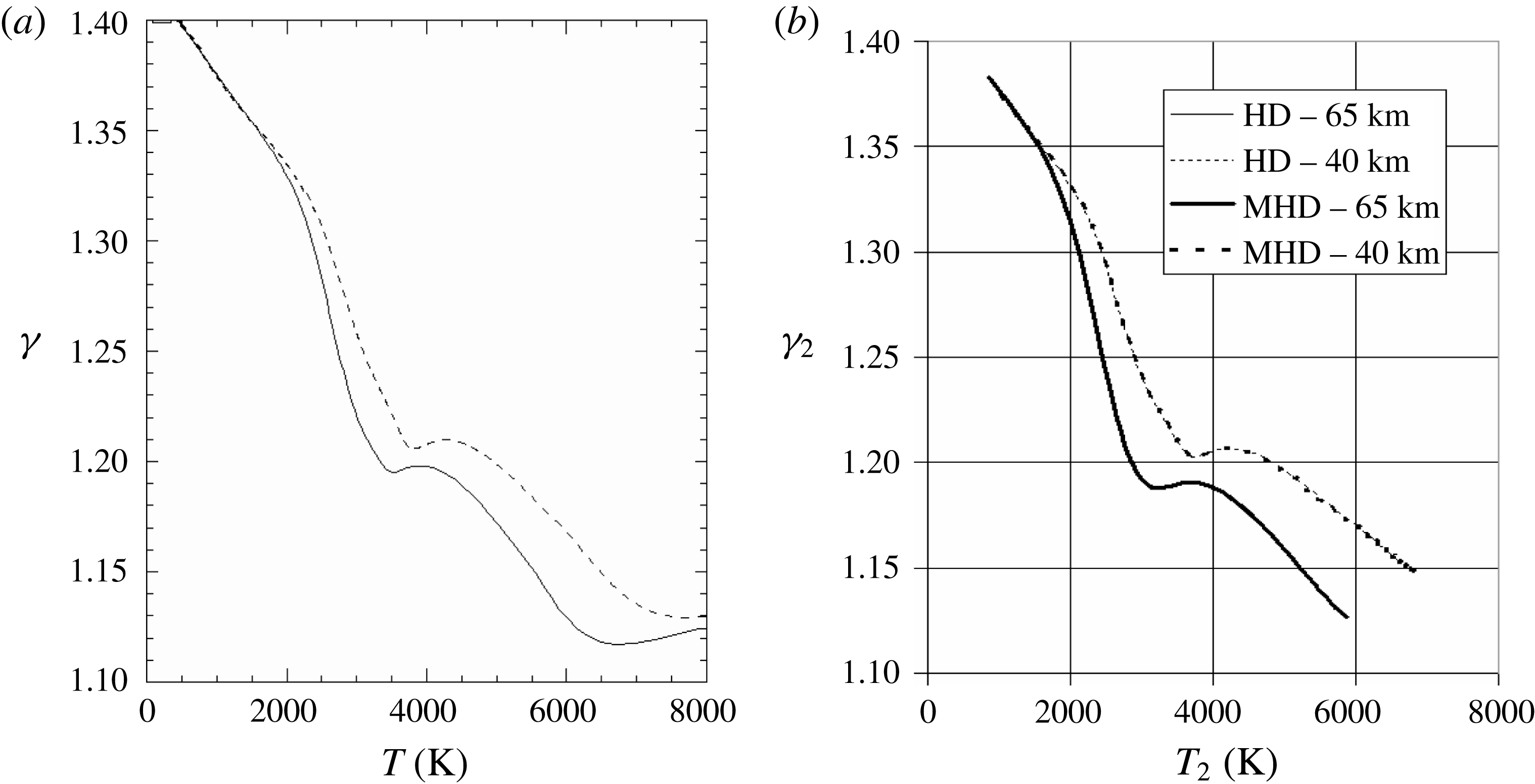
ions, thus yielding free electrons and producing electrical conductivity. We assumed equilibrium of the plasma and, since to calculate the pressure and density jump we need the isentropic exponent and conductivity behind the shock, we used a thermodynamic correlation model (Srinivasan, Tannehill & Weilmuenster Reference Srinivasan, Tannehill and Weilmuenster1987), providing a thermal state equation
 $T(p,\unicode[STIX]{x1D70C})$
, and a caloric state equation, providing the isentropic exponent
 $\unicode[STIX]{x1D6FE}(p,\unicode[STIX]{x1D70C})$
(tables 7, 8, 9 for
 $\unicode[STIX]{x1D6FE}(p,\unicode[STIX]{x1D70C})$
and tables 10, 11, 12 for
 $T(p,\unicode[STIX]{x1D70C})$
in Srinivasan et al. (Reference Srinivasan, Tannehill and Weilmuenster1987)). This model is an improved version of a former model (Tannehill & Mugge Reference Tannehill and Mugge1974).
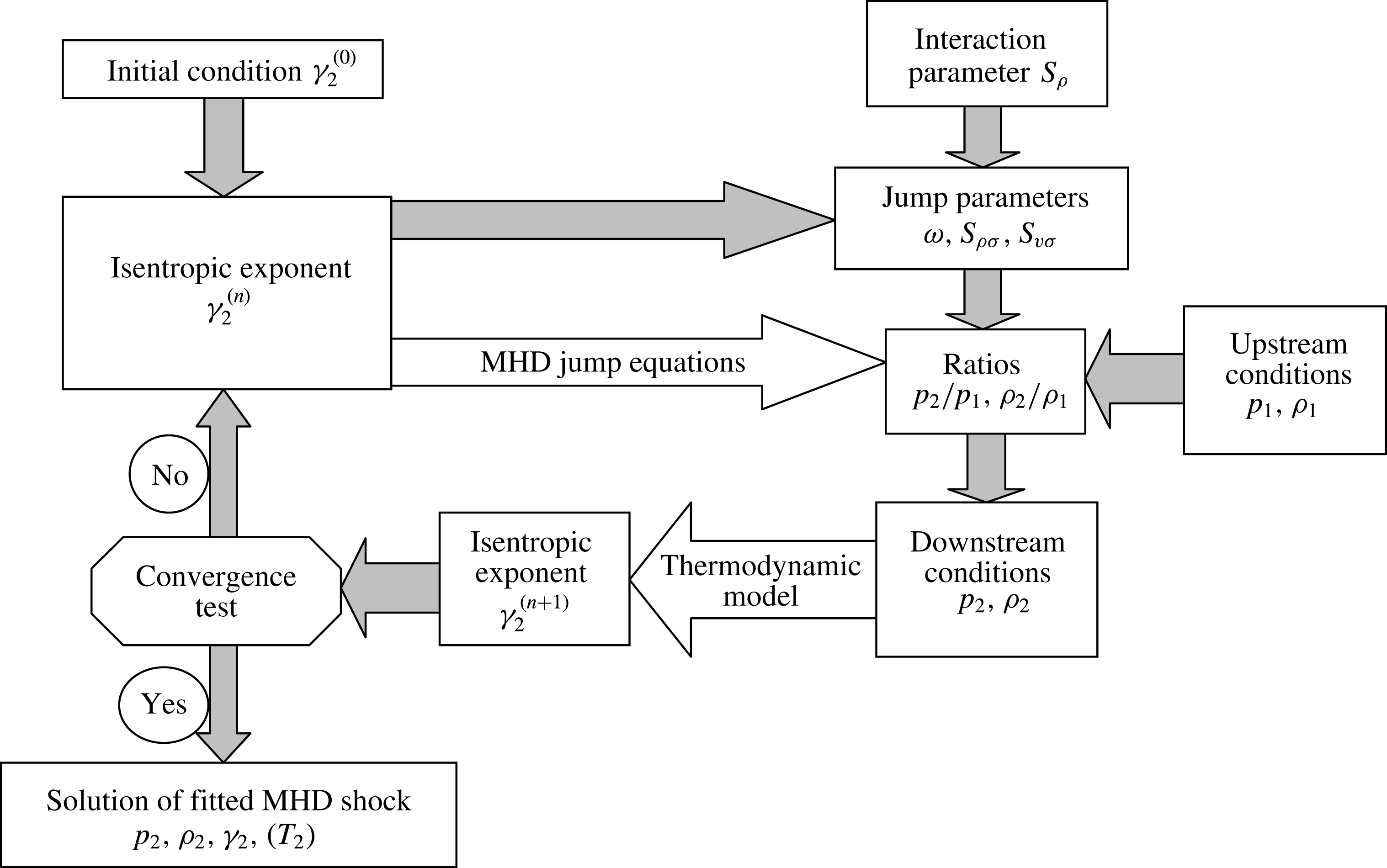
The shock is fitted by iteration of the isentropic exponent
 $\unicode[STIX]{x1D6FE}_{2}$
, and the algorithm is depicted in figure 3 with the interaction parameter
 $S_{\unicode[STIX]{x1D70C}}$
fixed. The convergence test at step
 $n$
is simply taken as
 $$\begin{eqnarray}\displaystyle \displaystyle \left|\frac{\unicode[STIX]{x1D6FE}_{2}^{\left(n\right)}-\unicode[STIX]{x1D6FE}_{2}^{\left(n-1\right)}}{\unicode[STIX]{x1D6FE}_{2}^{\left(n-1\right)}}\right|<\unicode[STIX]{x1D71B}, & & \displaystyle\end{eqnarray}$$
with the threshold value
 $\unicode[STIX]{x1D71B}=10^{-8}$
. The initial value is chosen as
 $\unicode[STIX]{x1D6FE}_{2}^{(0)}=1.4$
.
3.3 Numerical results
In order to show general features of resistive MHD shocks, we chose well suited situations combining the relative configurations of velocity and magnetic fields (
 $\unicode[STIX]{x1D712}_{1}$
,
 $\unicode[STIX]{x1D712}_{b}$
) and the state of the upstream medium, characterized by the physical conditions at an altitude of 40 km. The shock itself is characterized by the Mach number
 $M_{1}$
ranging from 5 to 30 and the microscopic interaction parameter
 $S_{\unicode[STIX]{x1D70C}}$
ranging from 0 to 0.1, since we must stay in the linear range (
 $S_{\unicode[STIX]{x1D70C}}\ll 1$
), and this parameter is small in re-entry applications.
Fitting procedure for a plane oblique MHD resistive shock.

Pressure (a) and mass density (b) ratios as functions of upstream Mach number
 $M_{1}$
and microscopic interaction parameter
 $S_{\unicode[STIX]{x1D70C}0}$
for the test case
 $\unicode[STIX]{x1D712}_{1}=20^{\circ }$
and
 $\unicode[STIX]{x1D712}_{b}=170^{\circ }$
for a plane oblique shock (
 $\unicode[STIX]{x1D6FC}=2$
;
 $\unicode[STIX]{x1D701}=10$
).

The two cases we consider,
 $\unicode[STIX]{x1D712}_{1}=20^{\circ }$
,
 $\unicode[STIX]{x1D712}_{b}=170^{\circ }$
and
 $\unicode[STIX]{x1D712}_{1}=60^{\circ }$
,
 $\unicode[STIX]{x1D712}_{b}=150^{\circ }$
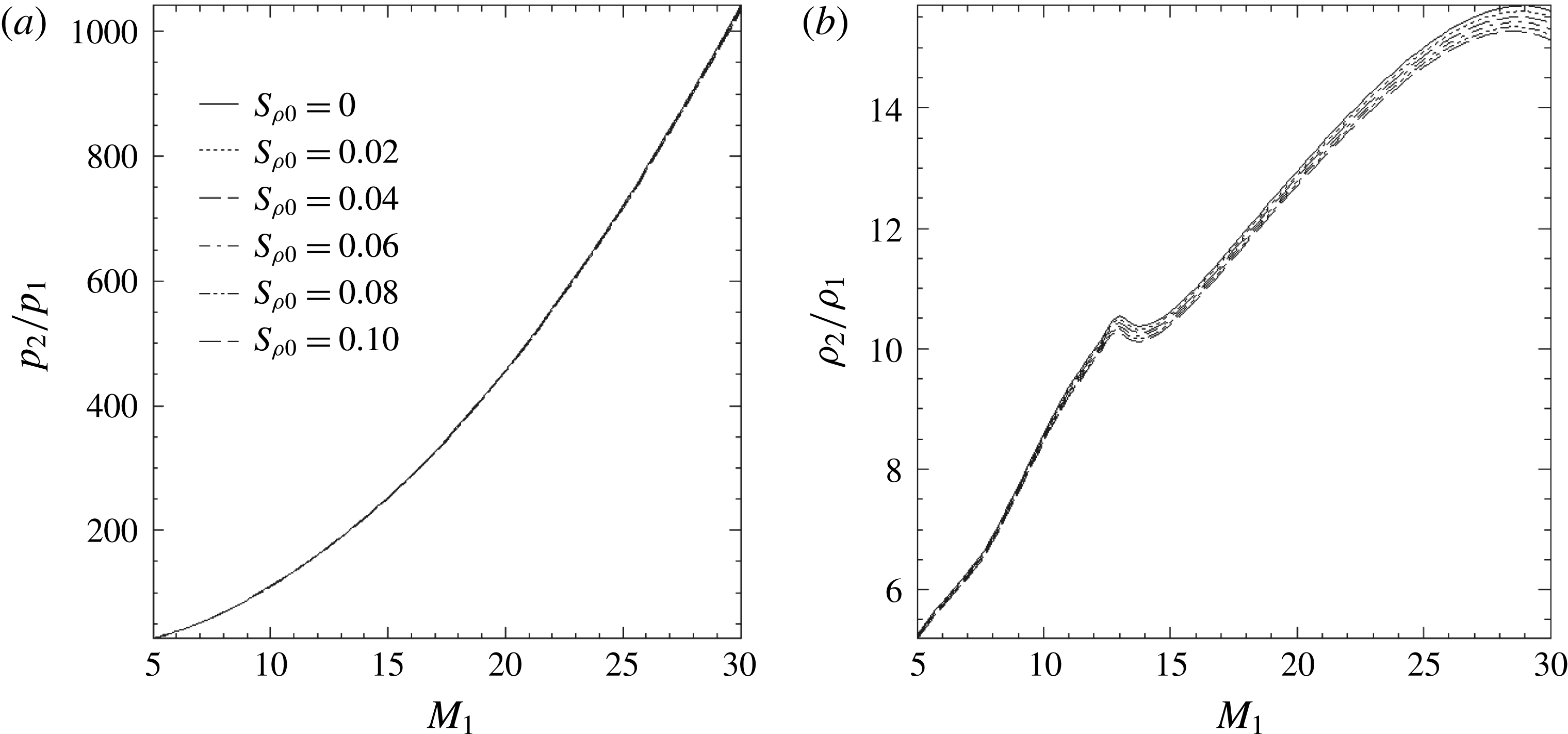
, depict two situations encountered before a blunt body. The results for case 1 (figure 4) show on one hand that the pressure ratio
 $p_{2}/p_{1}$
is practically independent of
 $S_{\unicode[STIX]{x1D70C}0}$
and increases quadratically with
 $M_{1}$
according to (3.9). On the other hand, the mass density ratio
 $\unicode[STIX]{x1D70C}_{2}/\unicode[STIX]{x1D70C}_{1}$
increases and a hump occurs at
 $M_{1}\approx 13$
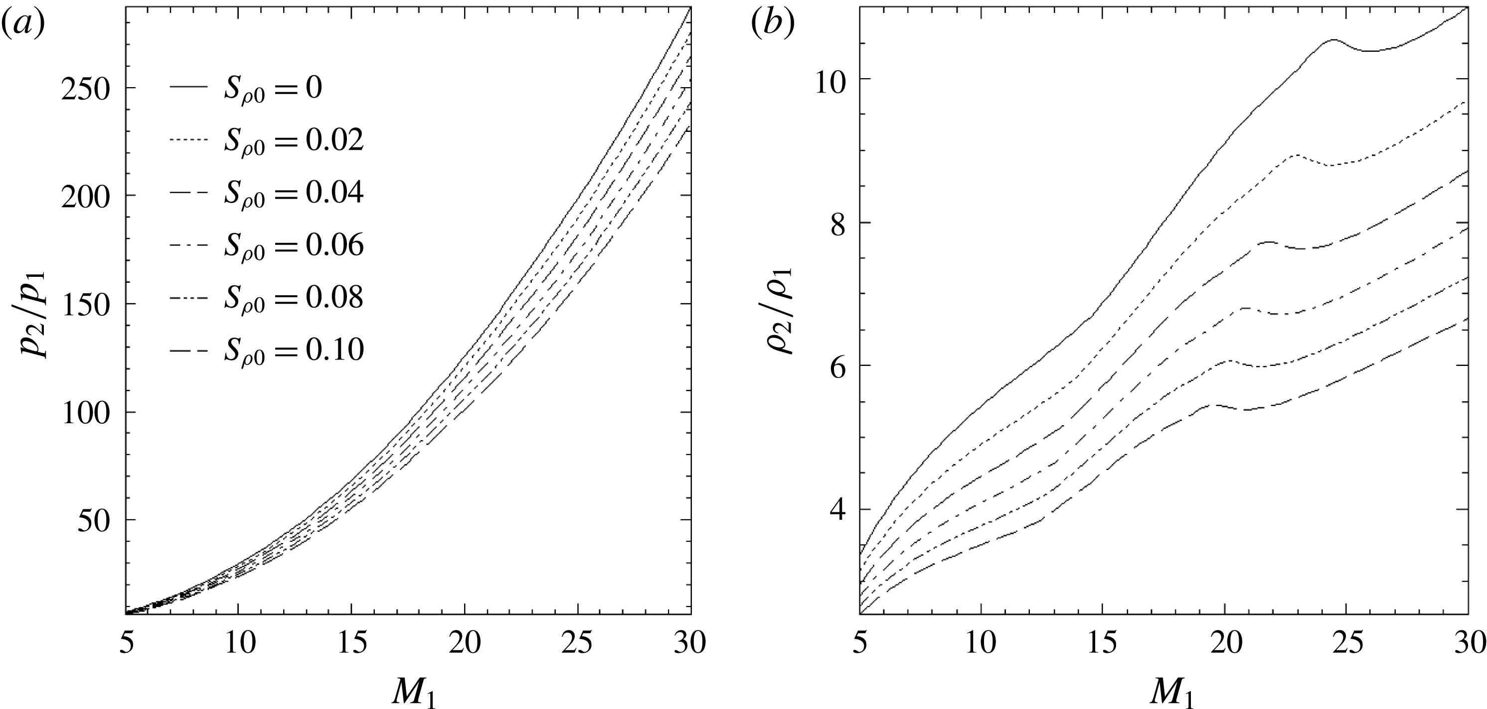
. In case 2 (figure 5), the pressure ratio curves can be slightly distinguished, and the mass density ratio curves are much more separated than in case 1. A hump occurs at
 $M_{1}\approx 23.5$
in the aerodynamic situation (
 $S_{\unicode[STIX]{x1D70C}}=0$
). Moreover, the level is lower in case 2, since the relative angle of the velocity and magnetic field vectors is smaller, indicating a smaller MHD effect.
The same as figure 4 for the test case
 $\unicode[STIX]{x1D712}_{1}=60^{\circ }$
and
 $\unicode[STIX]{x1D712}_{b}=150^{\circ }$
.

The hump appearing at
 $M_{1}\approx 13$
in case 1 is confirmed by earlier aerodynamic models of normal shocks in shock tubes (Glass & Hall Reference Glass and Hall1959) behind the detached shock ahead of a stratospheric blunt body in hypersonic re-entry flight (Huber Reference Huber1958). As stated in the reference papers, it reflects the resonance due to the dissociation of molecular oxygen and nitrogen in the temperature range 3500–4500 K. In case 2, the aerodynamic hump is shifted to
 $M_{1}\approx 23.5$
, because the variation of the incidence angle
 $\unicode[STIX]{x1D712}_{1}$
is equivalent to a shift of the critical Mach number, according to a similarity rule we shall explain in § 5.2,
 $$\begin{eqnarray}\displaystyle \displaystyle M_{11}\cos \unicode[STIX]{x1D712}_{11}=M_{12}\cos \unicode[STIX]{x1D712}_{12}, & & \displaystyle\end{eqnarray}$$
with
 $$\begin{eqnarray}\displaystyle \left.\begin{array}{@{}c@{}}M_{11}\approx 13,\\ \unicode[STIX]{x1D712}_{11}=20^{\circ },\\ M_{12}\approx 23.5,\\ \unicode[STIX]{x1D712}_{12}=60^{\circ }.\end{array}\right\} & & \displaystyle\end{eqnarray}$$
As
 $S_{\unicode[STIX]{x1D70C}}$
increases, the level of the density ratio is lowered and the abscissa of the hump is shifted to smaller Mach numbers (figure 5
b). This suggests the following inverse problem: from such plots of the variations of the mass density ratio, it might be possible to determine the microscopic interaction parameter
 $S_{\unicode[STIX]{x1D70C}}$
, and then, using measurements of the conductivity, magnetic field and normal mass rate, eventually estimate the length scale
 $\mathscr{L}_{\unicode[STIX]{x1D70C}}$
.
4 Application to blunt-body shock fitting
4.1 Fitting procedure
Here, we address the problem of the blunt body and work out a more complex procedure for fitting the various parameters behind the bow shock by applying the model of § 2 and neglecting curvature effects. The state of the air plasma generated behind the shock is described by the same correlation model as in the elementary fitting procedure of § 3.2.
Following other modellers (Bush Reference Bush1958; Coackley & Porter Reference Coackley and Porter1971; Otsu et al.
Reference Otsu, Matsuda, Abe and Konigorski2006; Otsu, Konigorski & Abe Reference Otsu, Konigorski and Abe2010), we used a power law of temperature for the conductivity, namely relation (A 5), with the constants
 $T_{0}=8000~\text{K}$
,
 $\unicode[STIX]{x1D70E}_{0}=731~\text{S}~\text{m}^{-1}$
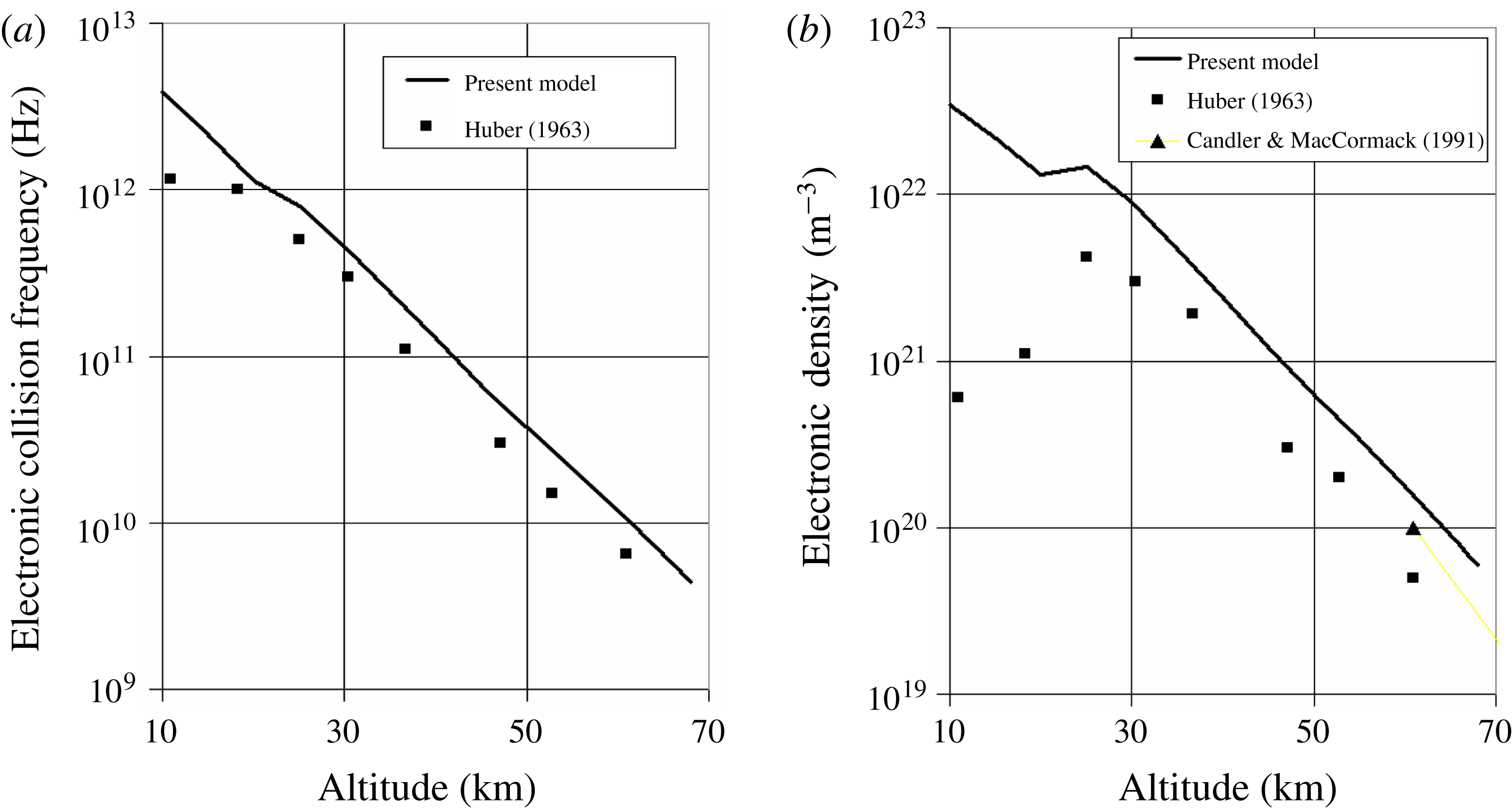
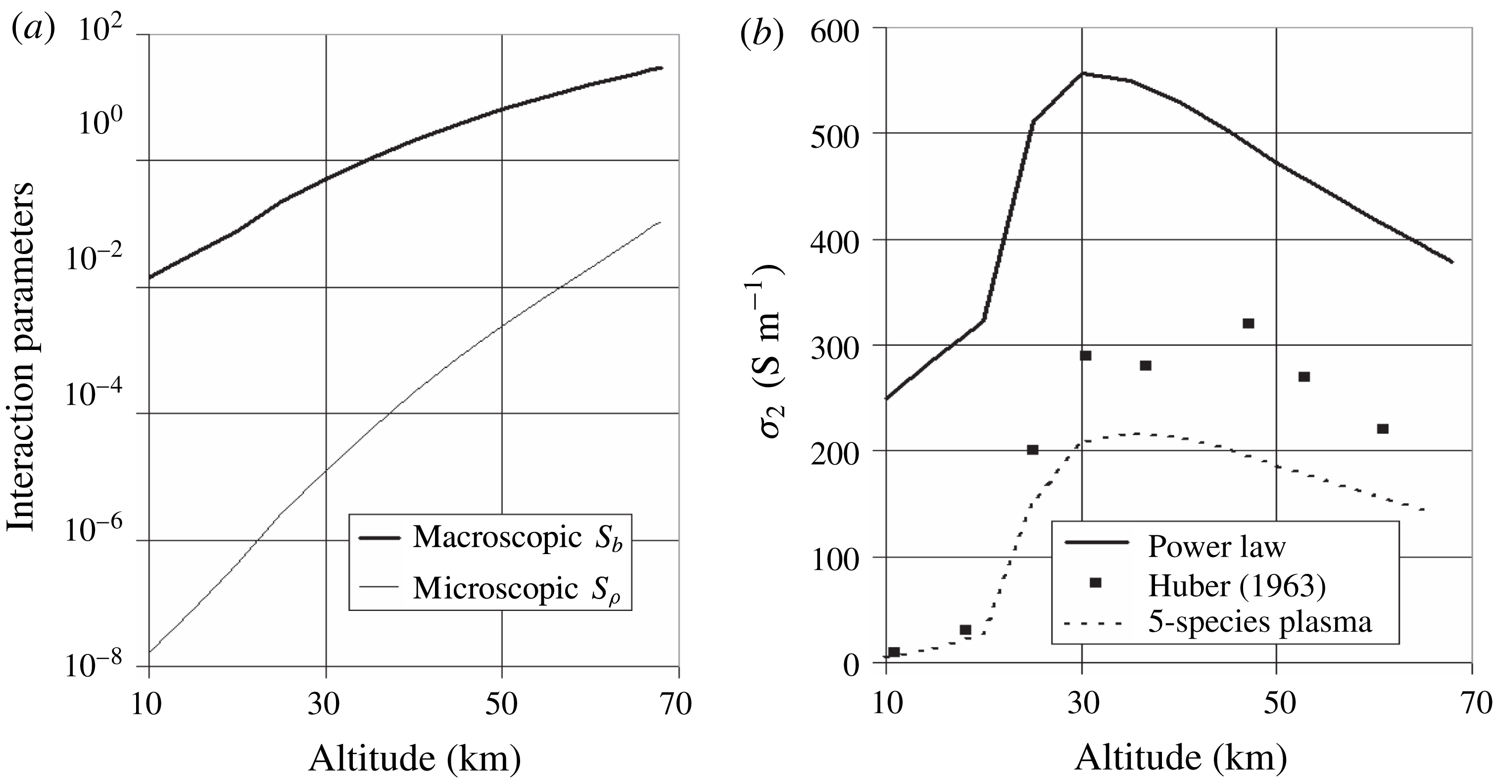
. Otherwise, former models have used a power law of velocity (Jarvinen Reference Jarvinen1965). We have checked that the conductivity obtained in this way is slightly overestimated compared with that produced by a plasma model (Viegas & Peng Reference Viegas and Peng1961; Sutton & Sherman Reference Sutton and Sherman2006; Bisek, Boyd & Poggie Reference Bisek, Boyd and Poggie2009), although other calculations in the same range of altitudes for nearly the same velocity (
 $V_{1}=8.5~\text{km}~\text{s}^{-1}$
) obtain several hundreds of
 $\text{S}~\text{m}^{-1}$
(Ericson & Maciulaitis Reference Ericson and Maciulaitis1964). Nevertheless, it has the great advantage of providing a simple dependence of the shock jumps on the microscopic interaction parameter
 $S_{\unicode[STIX]{x1D70C}}$
, as we showed in § 2.4.
Moreover, it is more accurate to use the magnetic field strength at the very location (
 $r,\unicode[STIX]{x1D703}$
) along the shock depending on the shock distance
 $\unicode[STIX]{x1D6FF}$
from the body nose, and, for this purpose, we also need to make iterations on
 $\unicode[STIX]{x1D6FF}$
in the MHD algorithm. The distance
 $\unicode[STIX]{x1D6FF}$
is related to the parameters
 $\unicode[STIX]{x1D700}$
and
 $\unicode[STIX]{x1D702}$
once a flow model is found. This will be explained in § 4.5.
The shock thickness
 $\mathscr{L}_{\unicode[STIX]{x1D70C}}$
, involved in the interaction parameter
 $S_{\unicode[STIX]{x1D70C}}$
, depends on the viscosity behind the shock through the expression (2.32) derived in appendix B and is therefore iterated since it depends on various parameters before and behind the shock.
The resulting algorithm, depicted in figure 7, turns out to be more complex than the one in § 3, since electrical conductivity, shock distance and thickness are also iterated. The fourfold convergence test at step
 $n$
is therefore taken as
 $$\begin{eqnarray}\displaystyle \displaystyle \left|\frac{\unicode[STIX]{x1D6FE}_{2}^{\left(n\right)}-\unicode[STIX]{x1D6FE}_{2}^{\left(n-1\right)}}{\unicode[STIX]{x1D6FE}_{2}^{\left(n-1\right)}}\right|<\unicode[STIX]{x1D71B},\quad \left|\frac{\unicode[STIX]{x1D70E}_{2}^{\left(n\right)}-\unicode[STIX]{x1D70E}_{2}^{\left(n-1\right)}}{\unicode[STIX]{x1D70E}_{2}^{\left(n-1\right)}}\right|<\unicode[STIX]{x1D71B}, & & \displaystyle\end{eqnarray}$$
 $$\begin{eqnarray}\displaystyle \left|\frac{\unicode[STIX]{x1D6FF}^{\left(n\right)}-\unicode[STIX]{x1D6FF}^{\left(n-1\right)}}{\unicode[STIX]{x1D6FF}^{\left(n-1\right)}}\right|<\unicode[STIX]{x1D71B},\quad \left|\frac{\mathscr{L}^{\left(n\right)}-\mathscr{L}^{\left(n-1\right)}}{\mathscr{L}^{\left(n-1\right)}}\right|<\unicode[STIX]{x1D71B}, & & \displaystyle\end{eqnarray}$$
with the same threshold value
 $\unicode[STIX]{x1D71B}=10^{-8}$
. Initial values are chosen such that
 $\unicode[STIX]{x1D6FE}_{2}^{(0)}=1.4$
,
 $\unicode[STIX]{x1D70E}_{2}^{(0)}=100~\text{S}~\text{m}^{-1}$
,
 $\unicode[STIX]{x1D6FF}^{(0)}=0.1R_{b}$
,
 $\mathscr{L}^{(0)}=(4/3)\unicode[STIX]{x1D707}_{1}/m$
. The convergence depends on the angles of velocity
 $\unicode[STIX]{x1D712}_{1}$
and magnetic field
 $\unicode[STIX]{x1D712}_{b}$
. In the pure aerodynamic case run for comparison, the convergence criterion reduces to the iteration on
 $\unicode[STIX]{x1D6FE}_{2}$
since the absence of magnetic field drops the influence of the conductivity, the shock distance and the shock thickness.
The viscosity, which is necessary for the estimation of the scale length (2.32) and the MHD parameters (2.23) and (2.25), is calculated in front of the shock by means of Sutherland’s formula for air (in Pl or
 $\text{kg}~\text{m}^{-1}~\text{s}^{-1}$
) (Sutherland Reference Sutherland1893),
 $$\begin{eqnarray}\displaystyle \displaystyle \unicode[STIX]{x1D707}(T)=1.7\times 10^{-5}\frac{T_{0}+T_{S}}{T+T_{S}}\left(\frac{T}{T_{0}}\right)^{3/2}, & & \displaystyle\end{eqnarray}$$
with the reference temperature
 $T_{0}=273~\text{K}$
and the Sutherland temperature for air
 $T_{S}=110~\text{K}$
. Behind the shock, the viscosity has been assumed to be independent of pressure and linear as a function of temperature below 10 000 K, on the basis of a published work for high-temperature air plasma (Capitelli, Colonna & D’Angola Reference Capitelli, Colonna and D’Angola2001).
At each angular position
 $\unicode[STIX]{x1D703}$
along the shock (figure 6), we shall locally approximate the shock as being a plane, i.e. neglect the curvature, and apply the jump conditions derived in the previous section. The angle
 $\unicode[STIX]{x1D712}_{1}$
of the upstream velocity is such that
 $$\begin{eqnarray}\displaystyle \displaystyle \unicode[STIX]{x1D712}_{1}=\unicode[STIX]{x1D703}_{n}. & & \displaystyle\end{eqnarray}$$
Moreover, the shock layer will be modelled in the vicinity of the symmetry axis with the approximation of a spherical shock. Therefore, we shall have the equivalence
 $$\begin{eqnarray}\displaystyle \displaystyle \unicode[STIX]{x1D703}_{n}=\unicode[STIX]{x1D703}. & & \displaystyle\end{eqnarray}$$
A simple analytical model of non-spherical shock assuming
 $\unicode[STIX]{x1D703}_{n}=\unicode[STIX]{x1D6FD}\unicode[STIX]{x1D703}(0\leqslant \unicode[STIX]{x1D6FD}\leqslant 1)$
and matching with the Mach angle for
 $M_{1}=23$
at
 $\unicode[STIX]{x1D703}=90^{\circ }$
shows that
 $\unicode[STIX]{x1D6FD}=0.97$
and thereupon proves the small deviation from sphericity. We shall now proceed to describe the topology of the magnetic, electric and velocity fields.
Geometrical sketch of an MHD bow shock ahead of an axisymmetric blunt body at hypersonic speed.

The fitting procedure for a resistive MHD bow shock.

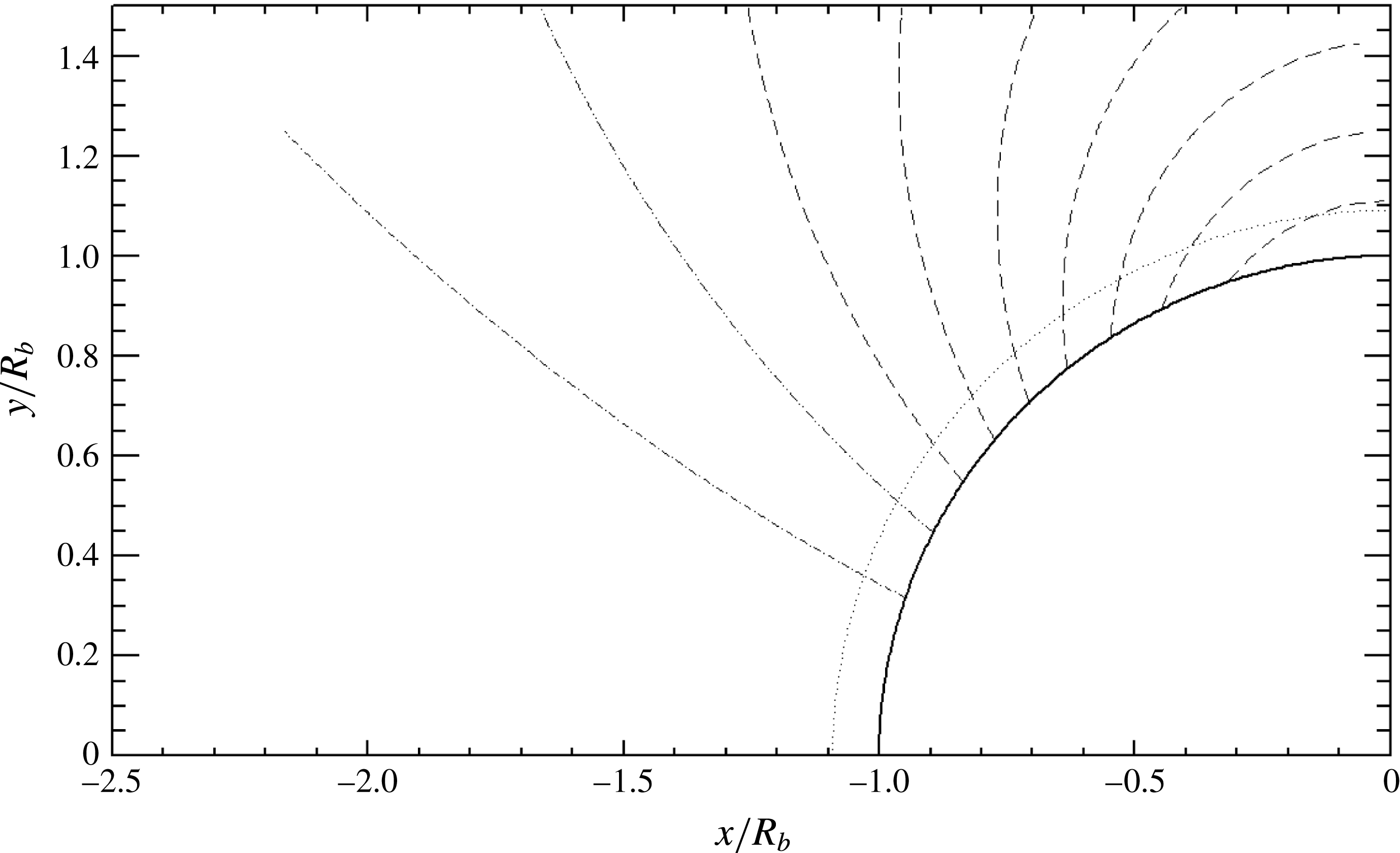
Magnetic lines of force (dashed lines). The shock (dotted line) is assumed to be spherical, at a distance
 $0.1R_{b}$
from the sphere in its initial position.

4.2 Magnetic and electric fields
A dipolar magnetic field
 $\boldsymbol{B}$
created by a magnet included in the body is applied to the spherical nose, with its axis parallel to the incident flow direction (Ziemer & Bush Reference Ziemer and Bush1958),
 $$\begin{eqnarray}\displaystyle \displaystyle B_{r}=2B_{0}\left(\frac{R_{b}}{r}\right)^{3}\cos \unicode[STIX]{x1D703},\quad B_{\unicode[STIX]{x1D711}}=0,\quad B_{\unicode[STIX]{x1D703}}=B_{0}\left(\frac{R_{b}}{r}\right)^{3}\sin \unicode[STIX]{x1D703}. & & \displaystyle\end{eqnarray}$$
This field is solenoidal (
 $\unicode[STIX]{x1D735}\boldsymbol{\cdot }\boldsymbol{B}=0$
) and vanishes at infinity. The magnetic strength
 $B$
is
 $$\begin{eqnarray}\displaystyle \displaystyle B=B_{0}\left(\frac{R_{b}}{r}\right)^{3}\sqrt{4\cos ^{2}\unicode[STIX]{x1D703}+\sin ^{2}\unicode[STIX]{x1D703}} & & \displaystyle\end{eqnarray}$$
and the moment
 $\mathscr{M}_{B}$
of the generating magnetic dipole is such that
 $$\begin{eqnarray}\displaystyle \displaystyle B_{0}=\frac{\unicode[STIX]{x1D707}_{0}\mathscr{M}_{B}}{4\unicode[STIX]{x03C0}R_{b}^{3}}. & & \displaystyle\end{eqnarray}$$
It can be shown that the above magnetic field is non-rotational everywhere (
 $\unicode[STIX]{x1D735}\times \boldsymbol{B}=\mathbf{0}$
).
Several magnetic lines of force have been drawn in figure 8. We notice that these lines are more and more inclined as we move away from the symmetry axis. Equation (4.7) shows that a nominal induction
 $B_{0}=0.5~\text{T}$
in relation (4.5) yields a magnetic field of 1 T at radius
 $R_{b}=0.15~\text{m}$
at the stagnation point on the body, and can be obtained with a magnet possessing a magnetic moment of
 $\mathscr{M}_{B}=16\,875~\text{A}~\text{m}^{2}$
.
Using (4.5), we obtain that
 $\unicode[STIX]{x1D712}_{b}$
is related to
 $\unicode[STIX]{x1D703}$
and
 $\unicode[STIX]{x1D703}_{n}$
by the equation
 $$\begin{eqnarray}\displaystyle \displaystyle \tan \left(\unicode[STIX]{x03C0}-\unicode[STIX]{x1D712}_{b}+\unicode[STIX]{x1D703}_{n}-\unicode[STIX]{x1D703}\right)=\frac{\tan \unicode[STIX]{x1D703}}{2}. & & \displaystyle\end{eqnarray}$$
The variations of
 $\unicode[STIX]{x1D712}_{b}$
as function of
 $\unicode[STIX]{x1D703}$
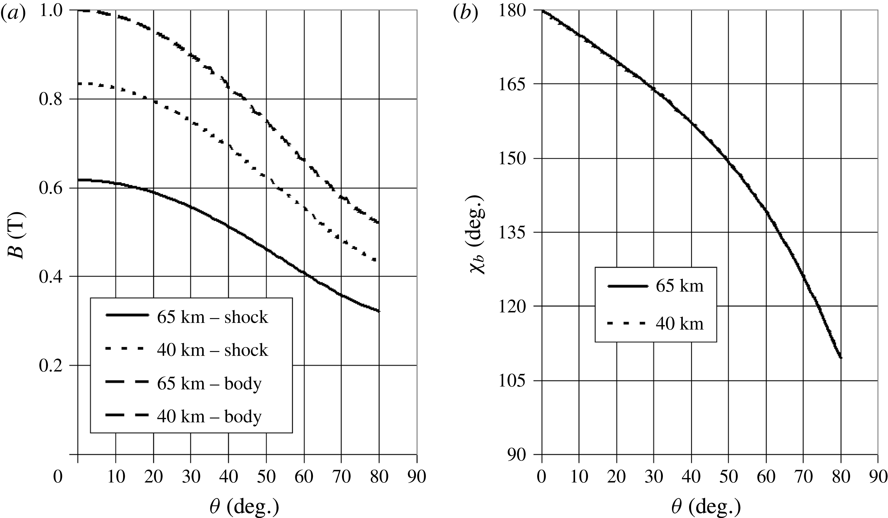
are displayed in figure 10(b) for a spherical shock (
 $\unicode[STIX]{x1D703}_{n}=\unicode[STIX]{x1D703}$
). They are nonlinear, but can be approximated by expanding (4.8) to third order in
 $\unicode[STIX]{x1D703}$
,
 $$\begin{eqnarray}\displaystyle \displaystyle \unicode[STIX]{x1D712}_{b}\approx \unicode[STIX]{x03C0}-\frac{\unicode[STIX]{x1D703}}{2}\left(1+\displaystyle \frac{\unicode[STIX]{x1D703}^{2}}{3}\right). & & \displaystyle\end{eqnarray}$$
We shall verify that the radial dependence of
 $B$
in (4.6) must be taken into account in the shock-fitting process.
As regards the electric field, without Hall effect, the condition
 $E=0$
in the set (2.8) still holds because of the axisymmetry. To prove this, we consider a closed path
 $\mathscr{C}$
and a closed surface
 $\mathscr{S}$
admitting
 $\mathscr{C}$
as boundary. Then, taking the circulation of
 $\boldsymbol{E}$
along
 $\mathscr{C}$
, using Stoke’s theorem and Maxwell’s stationary equation of induction (
 $\unicode[STIX]{x1D735}\times \boldsymbol{E}=\mathbf{0}$
), it is shown that the circulation of
 $\boldsymbol{E}$
vanishes. Since in axisymmetric geometry
 $\mathscr{C}$
may be chosen as a circle, we conclude that
 $\boldsymbol{E}=0$
.
4.3 Velocity field
We model the flow behind the shock as simply as possible in order to estimate how our jump relations generate the coupling of shock distance and thickness, which is a key parameter. To describe this flow, assumed to be steady and laminar, we use a formalism based on streamlines, along which the stream function
 $\unicode[STIX]{x1D713}$
is constant (Oguchi Reference Oguchi1960; Maslen Reference Maslen1964; Noori, Hosseini & Ebrahimi Reference Noori, Hosseini and Ebrahimi2009). It is possible to define a
 $\unicode[STIX]{x1D713}$
function even in compressible magnetohydrodynamics, since the continuity equation has the same form.
For the sake of simplicity, we consider a hypersonic motion with zero incidence, i.e. the incident flow is along the symmetry axis of the blunt body. In spherical coordinates suitable here for a blunt nose (figure 6), the velocity components are written as
 $$\begin{eqnarray}\displaystyle \displaystyle V_{r}=-\frac{\unicode[STIX]{x1D70C}_{0}}{\unicode[STIX]{x1D70C}}\frac{1}{r^{2}\sin \unicode[STIX]{x1D703}}\frac{\unicode[STIX]{x2202}\unicode[STIX]{x1D713}}{\unicode[STIX]{x2202}\unicode[STIX]{x1D703}},\quad V_{\unicode[STIX]{x1D703}}=\frac{\unicode[STIX]{x1D70C}_{0}}{\unicode[STIX]{x1D70C}}\displaystyle \frac{1}{r\sin \unicode[STIX]{x1D703}}\frac{\unicode[STIX]{x2202}\unicode[STIX]{x1D713}}{\unicode[STIX]{x2202}r}. & & \displaystyle\end{eqnarray}$$
The normalizing mass density
 $\unicode[STIX]{x1D70C}_{0}$
is a constant which makes
 $\unicode[STIX]{x1D713}$
of dimension
 $\text{m}^{3}~\text{s}^{-1}$
.
4.4 Jump conditions for the stream functions
In order to match upstream and downstream solutions at the shock, we derive jump conditions for the stream function, through their first derivatives. Let us relate the normal and tangential components of velocity to the magnitude
 $V$
and angle
 $\unicode[STIX]{x1D712}$
with the axis,
 $$\begin{eqnarray}\displaystyle \left.\begin{array}{@{}c@{}}u_{1}=V_{1}\cos \unicode[STIX]{x1D712}_{1},\\[6.0pt] v_{1}=V_{1}\sin \unicode[STIX]{x1D712}_{1},\\[6.0pt] u_{2}=V_{2}\cos \unicode[STIX]{x1D712}_{2},\\[6.0pt] v_{2}=V_{2}\sin \unicode[STIX]{x1D712}_{2}.\end{array}\right\} & & \displaystyle\end{eqnarray}$$
On both sides of the shock, the spherical components
 $V_{r}$
and
 $V_{\unicode[STIX]{x1D703}}$
are related to
 $V$
and the angle
 $\unicode[STIX]{x1D712}$
with respect to the shock normal and tangent by the relations
 $$\begin{eqnarray}\displaystyle \left.\begin{array}{@{}c@{}}V_{1r}=-V_{1}\cos \unicode[STIX]{x1D703},\\[6.0pt] V_{1\unicode[STIX]{x1D703}}=V_{1}\sin \unicode[STIX]{x1D703},\\[6.0pt] V_{2r}=-V_{2}\cos (\unicode[STIX]{x1D703}+\unicode[STIX]{x1D712}_{2}-\unicode[STIX]{x1D712}_{1}),\\[6.0pt] V_{2\unicode[STIX]{x1D703}}=V_{2}\sin (\unicode[STIX]{x1D703}+\unicode[STIX]{x1D712}_{2}-\unicode[STIX]{x1D712}_{1}).\end{array}\right\} & & \displaystyle\end{eqnarray}$$
Using the upstream Mach number
 $M_{1}$
(2.27) and relation (2.41), we recast (2.24) into
 $$\begin{eqnarray}\displaystyle \left.\begin{array}{@{}l@{}}u_{2}=\unicode[STIX]{x1D700}V_{1}\cos \unicode[STIX]{x1D712}_{1},\\[12.0pt] \displaystyle v_{2}=\left\{\left(d-\displaystyle \frac{bc}{a}\right)\sin \unicode[STIX]{x1D712}_{1}+\frac{c}{a}\unicode[STIX]{x1D700}\cos \unicode[STIX]{x1D712}_{1}\right\}V_{1}.\end{array}\right\} & & \displaystyle\end{eqnarray}$$
Then, making use of the magnetic parameter
 $\unicode[STIX]{x1D702}$
defined by (2.45), we derive the following simple relations for the velocity projections on the normal and the tangent to the shock:
 $$\begin{eqnarray}\displaystyle \left.\begin{array}{@{}l@{}}u_{2}=\unicode[STIX]{x1D700}u_{1},\\[6.0pt] v_{2}=\unicode[STIX]{x1D702}v_{1}.\end{array}\right\} & & \displaystyle\end{eqnarray}$$
Combining (4.11) and (4.14), we derive the important relations
 $$\begin{eqnarray}\displaystyle \left.\begin{array}{@{}l@{}}V_{2r}=-\unicode[STIX]{x1D700}V_{1}\cos \unicode[STIX]{x1D703},\\[6.0pt] V_{2\unicode[STIX]{x1D703}}=\unicode[STIX]{x1D702}V_{1}\sin \unicode[STIX]{x1D703}.\end{array}\right\} & & \displaystyle\end{eqnarray}$$
We notice the symmetrical roles played by
 $\unicode[STIX]{x1D700}$
and
 $\unicode[STIX]{x1D702}$
. In the non-magnetic case (
 $B=0$
,
 $a=d=1$
,
 $b=c=0$
),
 $\unicode[STIX]{x1D702}$
equals unity, and we recover the continuity of the tangential velocity.
Now, relating normal and tangential components to spherical coordinates by eliminating the amplitudes
 $V_{1}$
and
 $V_{2}$
, on taking the ratio of (4.11) and (4.12),
 $$\begin{eqnarray}\displaystyle \left.\begin{array}{@{}c@{}}\displaystyle \frac{V_{1r}}{u_{1}}=-\frac{\cos \unicode[STIX]{x1D703}}{\cos \unicode[STIX]{x1D712}_{1}},\\[12.0pt] \displaystyle \frac{V_{1\unicode[STIX]{x1D703}}}{v_{1}}=\frac{\sin \unicode[STIX]{x1D703}}{\sin \unicode[STIX]{x1D712}_{1}},\\[12.0pt] \displaystyle \frac{V_{2r}}{u_{2}}=-\frac{\cos \left(\unicode[STIX]{x1D703}+\unicode[STIX]{x1D712}_{2}-\unicode[STIX]{x1D712}_{1}\right)}{\cos \unicode[STIX]{x1D712}_{2}},\\[12.0pt] \displaystyle \frac{V_{2\unicode[STIX]{x1D703}}}{v_{2}}=\frac{\sin \left(\unicode[STIX]{x1D703}+\unicode[STIX]{x1D712}_{2}-\unicode[STIX]{x1D712}_{1}\right)}{\sin \unicode[STIX]{x1D712}_{2}},\end{array}\right\} & & \displaystyle\end{eqnarray}$$
and making use of (4.10) we finally get the general relations
 $$\begin{eqnarray}\displaystyle \left.\begin{array}{@{}l@{}}\displaystyle \left(\frac{\unicode[STIX]{x2202}\unicode[STIX]{x1D713}_{2}}{\unicode[STIX]{x2202}\unicode[STIX]{x1D703}}\right)_{c}=\left(\frac{\unicode[STIX]{x2202}\unicode[STIX]{x1D713}_{1}}{\unicode[STIX]{x2202}\unicode[STIX]{x1D703}}\right)_{c}\frac{\cos \unicode[STIX]{x1D712}_{1}}{\cos \unicode[STIX]{x1D712}_{2}}\frac{\cos \left(\unicode[STIX]{x1D703}+\unicode[STIX]{x1D712}_{2}-\unicode[STIX]{x1D712}_{1}\right)}{\cos \unicode[STIX]{x1D703}},\\[12.0pt] \displaystyle \left(\frac{\unicode[STIX]{x2202}\unicode[STIX]{x1D713}_{2}}{\unicode[STIX]{x2202}r}\right)_{c}=\left(\frac{\unicode[STIX]{x2202}\unicode[STIX]{x1D713}_{1}}{\unicode[STIX]{x2202}r}\right)_{c}\frac{\cos \unicode[STIX]{x1D712}_{1}}{\cos \unicode[STIX]{x1D712}_{2}}\frac{\sin \left(\unicode[STIX]{x1D703}+\unicode[STIX]{x1D712}_{2}-\unicode[STIX]{x1D712}_{1}\right)}{\sin \unicode[STIX]{x1D703}}.\end{array}\right\} & & \displaystyle\end{eqnarray}$$
For a spherical shock (
 $\unicode[STIX]{x1D712}_{1}=\unicode[STIX]{x1D703}$
), making use of (2.43), we can simplify this to
 $$\begin{eqnarray}\displaystyle \left.\begin{array}{@{}l@{}}\displaystyle \left(\frac{\unicode[STIX]{x2202}\unicode[STIX]{x1D713}_{2}}{\unicode[STIX]{x2202}\unicode[STIX]{x1D703}}\right)_{shock}=\left(\frac{\unicode[STIX]{x2202}\unicode[STIX]{x1D713}_{1}}{\unicode[STIX]{x2202}\unicode[STIX]{x1D703}}\right)_{shock},\\[12.0pt] \displaystyle \left(\frac{\unicode[STIX]{x2202}\unicode[STIX]{x1D713}_{2}}{\unicode[STIX]{x2202}r}\right)_{shock}=\frac{\unicode[STIX]{x1D702}}{\unicode[STIX]{x1D700}}\left(\frac{\unicode[STIX]{x2202}\unicode[STIX]{x1D713}_{1}}{\unicode[STIX]{x2202}r}\right)_{shock}.\end{array}\right\} & & \displaystyle\end{eqnarray}$$
We notice the continuity of the
 $\unicode[STIX]{x1D703}$
derivative of the stream function. The jump in the radial derivative is enhanced by the factor
 $\unicode[STIX]{x1D702}$
. For the non-magnetic flow, we have
 $\unicode[STIX]{x1D702}=1$
, and so we retrieve the hydrodynamic expression.
It is important to notice that the relations (4.17) and (4.18) are valid for any kind of flow, potential or not, that is described by
 $\unicode[STIX]{x1D713}_{2}$
. Moreover, the relations (4.17) hold for magnetic and non-magnetic flows as well.
4.5 Stream function and stand-off
Since the upstream flow is uniform, it is potential, i.e. curl-free, and its stream function is simply written as (Hayes & Probstein Reference Hayes and Probstein1959)
 $$\begin{eqnarray}\displaystyle \displaystyle \unicode[STIX]{x1D713}_{1}\left(r,\unicode[STIX]{x1D703}\right)=\frac{\unicode[STIX]{x1D70C}_{1}V_{1}}{2}r^{2}\sin ^{2}\unicode[STIX]{x1D703}. & & \displaystyle\end{eqnarray}$$
Using relations (4.10), we derive the velocity components before the shock,
 $$\begin{eqnarray}\displaystyle \displaystyle V_{1r}=-V_{1}\cos \unicode[STIX]{x1D703},\quad V_{1\unicode[STIX]{x1D711}}=0,\quad V_{1\unicode[STIX]{x1D703}}=V_{1}\sin \unicode[STIX]{x1D703}. & & \displaystyle\end{eqnarray}$$
As a first approximation, the downstream flow behind the shock might be assumed to be potential and to be described by a stream function of the following form (Kawamura Reference Kawamura1950, Reference Kawamura1952, Reference Kawamura1952--53):
 $$\begin{eqnarray}\displaystyle \displaystyle \unicode[STIX]{x1D713}_{2}\left(r,\unicode[STIX]{x1D703}\right)=\frac{\unicode[STIX]{x1D70C}_{1}V_{1}}{2}\displaystyle \frac{2\unicode[STIX]{x1D702}+\unicode[STIX]{x1D700}}{3\unicode[STIX]{x1D700}}\left(1-\frac{R_{b}^{3}}{r^{3}}\right)r^{2}\sin ^{2}\unicode[STIX]{x1D703}, & & \displaystyle\end{eqnarray}$$
which we derived using boundary conditions (4.18). Without magnetic field (
 $\unicode[STIX]{x1D702}=1$
), the aerodynamic solution is recovered (Kawamura Reference Kawamura1950, Reference Kawamura1952, Reference Kawamura1952--53), which was formerly accepted as a good approximation, in agreement with the then observed supersonic flows (Van Dyke Reference Van Dyke1958).
Nevertheless, vorticity is generated behind a curved aerodynamic shock (Hida Reference Hida1953; Hayes Reference Hayes1957; Lighthill Reference Lighthill1957), or even behind a plane MHD shock, as we have shown in appendix C. An MHD vorticity jump has been calculated for a curved shock, but in ideal magnetohydrodynamics (Sharma & Ram Reference Sharma and Ram1971). Moreover, the potential assumption fails at high Mach number and it leads to an underestimated shock stand-off.
Better approximations are provided by Lighthill’s model in aerodynamics (Lighthill Reference Lighthill1957) and Wu’s model in magnetohydrodynamics (Wu Reference Wu1960). This kind of model assumes inviscid flow and constant mass density behind the shock. The extension of Lighthill’s model to magnetohydrodynamics with the assumption of constant conductivity leads to a vorticity jump of the following form at the shock (Wu Reference Wu1960; Poggie & Gaitonde Reference Poggie and Gaitonde2002):
 $$\begin{eqnarray}\displaystyle \displaystyle [\unicode[STIX]{x1D6FA}_{\unicode[STIX]{x1D711}}]=-\frac{(1-\unicode[STIX]{x1D700})^{2}}{\unicode[STIX]{x1D700}}\frac{V_{\unicode[STIX]{x1D703}2}}{R_{s}}-\displaystyle \frac{F_{\unicode[STIX]{x1D703}}}{\unicode[STIX]{x1D70C}_{2}V_{r2}}. & & \displaystyle\end{eqnarray}$$
From this expression, since the magnetic force component
 $F_{\unicode[STIX]{x1D703}}$
is expressed as
 $$\begin{eqnarray}\displaystyle \displaystyle F_{\unicode[STIX]{x1D703}}=\unicode[STIX]{x1D70E}(V_{r}B_{\unicode[STIX]{x1D703}}-V_{\unicode[STIX]{x1D703}}B_{r})B_{r}, & & \displaystyle\end{eqnarray}$$
assuming a spherical shock (
 $\unicode[STIX]{x1D712}_{1}=\unicode[STIX]{x1D703}$
), using the expressions (4.15) and the magnetic field components (4.5) on the shock (
 $r=R_{s}$
), in a first step, we express the total vorticity behind the shock (
 $\unicode[STIX]{x1D6FA}_{\unicode[STIX]{x1D711}1}=0$
) as
 $$\begin{eqnarray}\displaystyle \displaystyle \unicode[STIX]{x1D6FA}_{\unicode[STIX]{x1D711}2}=-\unicode[STIX]{x1D702}\frac{\left(1-\unicode[STIX]{x1D700}\right)^{2}}{\unicode[STIX]{x1D700}}\frac{V_{1}}{R_{s}}\sin \unicode[STIX]{x1D703}-2\left(2\unicode[STIX]{x1D702}+\unicode[STIX]{x1D700}\right)\displaystyle \frac{\unicode[STIX]{x1D70E}_{2}B_{0}^{2}}{\unicode[STIX]{x1D70C}_{1}}\left(\frac{R_{b}}{R_{s}}\right)^{6}\sin \unicode[STIX]{x1D703}\cos \unicode[STIX]{x1D703}. & & \displaystyle\end{eqnarray}$$
This expression is formally consistent with the non-dimensional result published in a reference work (Poggie & Gaitonde Reference Poggie and Gaitonde2002). Then, in a second step, following Lighthill’s procedure, we derive the equation of the vorticity,
 $$\begin{eqnarray}\displaystyle & & \displaystyle \displaystyle \frac{\unicode[STIX]{x2202}^{2}\unicode[STIX]{x1D713}}{\unicode[STIX]{x2202}r^{2}}+\frac{\sin \unicode[STIX]{x1D703}}{r^{2}}\frac{\unicode[STIX]{x2202}}{\unicode[STIX]{x2202}\unicode[STIX]{x1D703}}\left(\frac{1}{\sin \unicode[STIX]{x1D703}}\frac{\unicode[STIX]{x2202}\unicode[STIX]{x1D713}}{\unicode[STIX]{x2202}\unicode[STIX]{x1D703}}\right)\nonumber\\ \displaystyle & & \displaystyle \quad =\,\unicode[STIX]{x1D70C}_{1}V_{1}\left\{\unicode[STIX]{x1D702}\frac{\left(1-\unicode[STIX]{x1D700}\right)^{2}}{\unicode[STIX]{x1D700}^{2}}+2S_{b}\left(2\frac{\unicode[STIX]{x1D702}}{\unicode[STIX]{x1D700}}+1\right)q^{5}\cos \unicode[STIX]{x1D703}\right\}\frac{r^{2}}{R_{s}^{2}}\sin ^{2}\unicode[STIX]{x1D703}.\end{eqnarray}$$
After defining the macroscopic interaction parameter
 $S_{b}$
built on the body nose radius
 $R_{b}$
,
 $$\begin{eqnarray}\displaystyle \displaystyle S_{b}=\frac{\unicode[STIX]{x1D70E}_{2}B_{0}^{2}R_{b}}{\unicode[STIX]{x1D70C}_{1}V_{1}}, & & \displaystyle\end{eqnarray}$$
and the ratio
 $$\begin{eqnarray}\displaystyle \displaystyle q=\frac{R_{b}}{R_{s}}, & & \displaystyle\end{eqnarray}$$
we assume that the stream function solution
 $\unicode[STIX]{x1D713}_{2}$
can be cast as the sum of two terms,
 $$\begin{eqnarray}\displaystyle \displaystyle \unicode[STIX]{x1D713}_{2}=\unicode[STIX]{x1D713}_{2}^{(0)}+S_{b}\unicode[STIX]{x1D713}_{2}^{(1)}. & & \displaystyle\end{eqnarray}$$
The first term
 $\unicode[STIX]{x1D713}_{2}^{(0)}$
corresponds to Lighthill’s solution of (4.25) with the first term of the right-hand side, involving the correcting magnetic factor
 $\unicode[STIX]{x1D702}$
, such that
 $$\begin{eqnarray}\displaystyle \displaystyle \frac{\unicode[STIX]{x1D713}_{2}^{(0)}(r,\unicode[STIX]{x1D703})}{\unicode[STIX]{x1D70C}_{1}V_{1}R_{s}^{2}} & = & \displaystyle \unicode[STIX]{x1D702}\frac{\left(1-\unicode[STIX]{x1D700}\right)^{2}}{10\unicode[STIX]{x1D700}^{2}}\left(\frac{r}{R_{s}}\right)^{4}+\frac{1}{3}\left\{\frac{1}{2}+\frac{\unicode[STIX]{x1D702}}{\unicode[STIX]{x1D700}}-\unicode[STIX]{x1D702}\displaystyle \frac{(1-\unicode[STIX]{x1D700})^{2}}{2\unicode[STIX]{x1D700}^{2}}\right\}\left(\frac{r}{R_{s}}\right)^{2}\nonumber\\ \displaystyle & & \displaystyle +\,\frac{1}{3}\left\{1-\frac{\unicode[STIX]{x1D702}}{\unicode[STIX]{x1D700}}+\unicode[STIX]{x1D702}\frac{(1-\unicode[STIX]{x1D700})^{2}}{5\unicode[STIX]{x1D700}^{2}}\right\}\frac{R_{s}}{r}.\end{eqnarray}$$
In the non-magnetic case (
 $S_{b}=0$
,
 $\unicode[STIX]{x1D702}=1$
), this first term
 $\unicode[STIX]{x1D713}_{2}^{(0)}$
yields exactly Lighthill’s solution,
 $$\begin{eqnarray}\displaystyle \displaystyle \unicode[STIX]{x1D713}_{2}(r,\unicode[STIX]{x1D703}) & = & \displaystyle \frac{\unicode[STIX]{x1D70C}_{1}V_{1}R_{s}^{2}}{30\unicode[STIX]{x1D700}^{2}}\left\{3\left(1-\unicode[STIX]{x1D700}\right)^{2}\left({\displaystyle \frac{r}{R_{s}}}\right)^{4}-5\left(1-4\unicode[STIX]{x1D700}\right)\left(\frac{r}{R_{s}}\right)^{2}\right.\nonumber\\ \displaystyle & & \displaystyle \left.+\,2\left(1-\unicode[STIX]{x1D700}\right)\left(1-6\unicode[STIX]{x1D700}\right)\frac{R_{s}}{r}\right\}\sin ^{2}\unicode[STIX]{x1D703}.\end{eqnarray}$$
The shock distance
 $\unicode[STIX]{x1D6FF}$
defined by
 $$\begin{eqnarray}\displaystyle \displaystyle \unicode[STIX]{x1D6FF}=\frac{R_{s}-R_{b}}{R_{b}} & & \displaystyle\end{eqnarray}$$
is therefore such that
 $$\begin{eqnarray}\displaystyle \displaystyle \unicode[STIX]{x1D6FF}=\frac{1}{q}-1, & & \displaystyle\end{eqnarray}$$
and
 $q$
is the solution of the equation
 $$\begin{eqnarray}\displaystyle \displaystyle \unicode[STIX]{x1D713}_{2}\left(R_{b}\right)=0; & & \displaystyle\end{eqnarray}$$
that is,
 $$\begin{eqnarray}\displaystyle \displaystyle \unicode[STIX]{x1D702}\frac{(1-\unicode[STIX]{x1D700})^{2}}{10\unicode[STIX]{x1D700}}q^{5}+\frac{1}{3}\left\{{\displaystyle \frac{\unicode[STIX]{x1D700}}{2}}+\unicode[STIX]{x1D702}-\unicode[STIX]{x1D702}\frac{(1-\unicode[STIX]{x1D700})^{2}}{2\unicode[STIX]{x1D700}}\right\}q^{3}+\frac{1}{3}\left\{\unicode[STIX]{x1D700}-\unicode[STIX]{x1D702}+\unicode[STIX]{x1D702}\frac{(1-\unicode[STIX]{x1D700})^{2}}{5\unicode[STIX]{x1D700}}\right\}=0. & & \displaystyle\end{eqnarray}$$
Looking for a simple perturbation
 $\unicode[STIX]{x1D713}_{2}^{(1)}$
in
 $\sin ^{2}\unicode[STIX]{x1D703}$
by assuming
 $\cos \unicode[STIX]{x1D703}\approx 1$
in the second term of the vorticity expression, equation (4.25), leads to a sixth-degree equation for
 $q$
instead of (4.34), which has no real solution with the prescribed physical conditions at 40 and 65 km. This point is a question to be considered in future work.
Obtained by a different approach based on the Newtonian pressure relation, Lykoudis’s MHD solution gives the following expression for the MHD distance
 $\unicode[STIX]{x1D6FF}$
(Lykoudis Reference Lykoudis1961):
 $$\begin{eqnarray}\displaystyle \displaystyle \frac{\unicode[STIX]{x1D6FF}}{\unicode[STIX]{x1D6FF}_{0}}\approx \frac{S_{b}}{2}\sqrt{\frac{3}{8}\unicode[STIX]{x1D700}}+\sqrt{1+{\displaystyle \frac{3\unicode[STIX]{x1D700}S_{b}^{2}}{32}}}, & & \displaystyle\end{eqnarray}$$
with the non-magnetic distance
 $\unicode[STIX]{x1D6FF}_{0}$
such that
 $$\begin{eqnarray}\displaystyle \displaystyle \frac{\unicode[STIX]{x1D6FF}_{0}}{R_{b}}=\frac{\unicode[STIX]{x1D700}}{1+\sqrt{\frac{8}{3}\unicode[STIX]{x1D700}}}, & & \displaystyle\end{eqnarray}$$
and the macroscopic interaction parameter
 $S_{b}$
defined by (4.26).
Lighthill’s aerodynamical solution, assuming constant mass density behind the shock and a perfect gas, leads to the following expansion to second order (Lighthill Reference Lighthill1957; Hayes & Probstein Reference Hayes and Probstein1959):
 $$\begin{eqnarray}\displaystyle \displaystyle \frac{\unicode[STIX]{x1D6FF}_{0}}{R_{b}}\approx \unicode[STIX]{x1D700}\left(1-\sqrt{\frac{8}{3}\unicode[STIX]{x1D700}}+3\unicode[STIX]{x1D700}\right). & & \displaystyle\end{eqnarray}$$
It can be checked that the aerodynamic distance obtained by the formulae (4.36) and (4.37) give results slightly smaller and larger than the solution given by (4.34) with
 $\unicode[STIX]{x1D702}=1$
. Therefore, we used the solution to (4.34) with
 $\unicode[STIX]{x1D702}=1$
for
 $\unicode[STIX]{x1D6FF}_{0}$
.
Since the ratio
 $\sin \unicode[STIX]{x1D712}_{b}/\text{sin}~\unicode[STIX]{x1D712}_{1}$
is an indeterminate form 0/0 on the stagnation line (
 $\unicode[STIX]{x1D712}_{1}=0$
and
 $\unicode[STIX]{x1D712}_{b}=0$
), the limit of
 $\unicode[STIX]{x1D702}$
on the stagnation line (
 $\unicode[STIX]{x1D703}\rightarrow 0$
) by (2.45) using the expansion (4.9) yields
 $$\begin{eqnarray}\displaystyle \displaystyle \unicode[STIX]{x1D702}\approx \frac{1}{1+S_{v\unicode[STIX]{x1D70E}0}}\left(1-\frac{\unicode[STIX]{x1D700}S_{\unicode[STIX]{x1D70C}\unicode[STIX]{x1D70E}0}}{2}\right), & & \displaystyle\end{eqnarray}$$
with the ‘normal’ interaction parameters corresponding to
 $\unicode[STIX]{x1D712}_{1}=0$
,
 $$\begin{eqnarray}\displaystyle \displaystyle S_{\unicode[STIX]{x1D70C}\unicode[STIX]{x1D70E}0}=\frac{\unicode[STIX]{x1D70E}_{2}B^{2}\mathscr{L}_{\unicode[STIX]{x1D70C}\unicode[STIX]{x1D70E}}}{m_{0}},\quad \displaystyle S_{v\unicode[STIX]{x1D70E}0}=\frac{\unicode[STIX]{x1D70E}_{2}B^{2}\mathscr{L}_{v\unicode[STIX]{x1D70E}}}{m_{0}},\quad m_{0}=\unicode[STIX]{x1D70C}_{1}V_{1}. & & \displaystyle\end{eqnarray}$$
5 Application to atmospheric entry
5.1 Results
The calculation was made with
 $\unicode[STIX]{x1D6FE}_{1}=1.4$
and
 $B_{0}=0.5~\text{T}$
for a hypersonic shock at stratospheric heights of 40 and 65 km, where significantly different ambient physical conditions are found (table 2). The large discrepancies in the kinematic viscosity
 $\unicode[STIX]{x1D708}_{1}$
result in very different mean free paths
 $\ell _{1}$
and shock thicknesses
 $\mathscr{L}_{\unicode[STIX]{x1D70C}}$
estimated by means of relations (2.30) and (2.32). In both cases, we assumed an exponent of
 $\unicode[STIX]{x1D6FC}=2$
and a factor of
 $\unicode[STIX]{x1D701}=10$
.
Physical conditions on the axis before (1) and behind (2) the shock of a re-entry blunt body at 40 km and 65 km in our calculations (
 $B_{0}=0.5~\text{T}$
;
 $\unicode[STIX]{x1D6FE}_{1}=1.40$
). Magnetic and non-magnetic results are coincident on the symmetry axis.

As the spherical assumption is only valid not far from the symmetry axis, we use the complete scheme of figure 7 with all four test ratios (4.1) only for
 $\unicode[STIX]{x1D712}_{1}=0$
on the symmetry axis. For
 $\unicode[STIX]{x1D712}_{1}\neq 0$
, we keep the shock distance
 $\unicode[STIX]{x1D6FF}$
constant and equal to its value at
 $\unicode[STIX]{x1D712}_{1}=0$
and fit only
 $\unicode[STIX]{x1D6FE}_{2}$
,
 $\unicode[STIX]{x1D70E}_{2}$
and
 $\mathscr{L}_{\unicode[STIX]{x1D70C}}$
. The aerodynamic behaviour is found with application of the fitting procedure only on
 $\unicode[STIX]{x1D6FE}_{2}$
.
Plots displaying typical variations of convergence test ratios (4.4) as functions of iteration number at 65 km on the symmetry axis (figure 9) show that convergence is easily reached within around 10 iterations for
 $\unicode[STIX]{x1D6FE}_{2}$
,
 $\unicode[STIX]{x1D70E}_{2}$
and
 $\mathscr{L}_{\unicode[STIX]{x1D70C}}$
, but only within around 20 iterations for
 $\unicode[STIX]{x1D6FF}$
.
The angular variations of the magnetic field strength are displayed in figure 10(a) for
 $0<\unicode[STIX]{x1D712}_{1}<80^{\circ }$
. They depend upon the shock stand-off, and the field is therefore stronger on the shock at 40 km than at 65 km because the shock distance is larger at 65 km than at 40 km.
Figure 11 displays the variations of pressure, temperature, isentropic exponent, Mach number and velocity angle behind the shock as functions of
 $\unicode[STIX]{x1D712}_{1}$
in the same range. The pressures profiles (a) have a classic cosine shape, the aerodynamic and MHD profiles being coincident at 40 km and 65 km, in agreement with the analysis of § 3 (figures 4
a and 5
a).
Convergence plots of the isentropic exponent
 $\unicode[STIX]{x1D6FE}_{2}$
(a), electrical conductivity
 $\unicode[STIX]{x1D70E}_{2}$
(b), relative shock stand-off
 $\unicode[STIX]{x1D6FF}/R_{b}$
(c) and shock thickness
 $\mathscr{L}_{\unicode[STIX]{x1D70C}}$
(d) in resistive MHD shock fitting with the procedure of figure 7 for physical conditions at 65 km on the symmetry axis of a resistive MHD bow shock (
 $\unicode[STIX]{x1D712}_{1}=\unicode[STIX]{x1D703}=0^{\circ }$
;
 $\unicode[STIX]{x1D712}_{b}=180^{\circ }$
).

Magnetic field strength on the shock and on the body surface (a), and angle
 $\unicode[STIX]{x1D712}_{b}$
of the magnetic field vector with respect to the shock normal (b) as functions of the polar angle
 $\unicode[STIX]{x1D703}$
for a spherical shock and the axial dipolar magnetic field of figure 8 (
 $B_{0}=0.5~\text{T}$
).

Pressure ratio
 $p_{2}/p_{1}$
(a), temperature
 $T_{2}$
(b), mass density ratio
 $\unicode[STIX]{x1D70C}_{2}/\unicode[STIX]{x1D70C}_{1}$
(c), isentropic exponent
 $\unicode[STIX]{x1D6FE}_{2}$
(d), Mach number (e) and deflection angle
 $\unicode[STIX]{x1D712}_{2}-\unicode[STIX]{x1D712}_{1}$
(f) as functions of upstream velocity angle
 $\unicode[STIX]{x1D712}_{1}$
behind a bow shock (
 $B_{0}=0.5~\text{T}$
).

Electrical conductivity
 $\unicode[STIX]{x1D70E}_{2}$
(a), magnetic parameter
 $\unicode[STIX]{x1D702}$
(b), shock thickness
 $\mathscr{L}_{\unicode[STIX]{x1D70C}}$
(c) and microscopic interaction parameter
 $S_{\unicode[STIX]{x1D70C}}$
(d) as functions of upstream velocity angle
 $\unicode[STIX]{x1D712}_{1}$
behind a resistive MHD bow shock (
 $B_{0}=0.5~\text{T}$
).

Temperature profiles (figure 11
b), showing a kind of cosine shape, nearly coincide at 40 km, whereas at 65 km the MHD profile lies slightly above the aerodynamic profile (
 $\unicode[STIX]{x0394}T_{2}\approx 111~\text{K}$
at
 $\unicode[STIX]{x1D712}_{1}=50^{\circ }$
). Consequently, the mass density profiles (figure 11
c) are coincident at 40 km, whereas the MHD profile lies beneath the aerodynamic one at 65 km (
 ${\approx}5.3\,\%$
at
 $\unicode[STIX]{x1D712}_{1}=50^{\circ }$
).
The isentropic exponent (figure 11
d) is of order 1.1 in the vicinity of the nose axis and increases as
 $\unicode[STIX]{x1D712}_{1}$
increases, with a parabolic branch. As mentioned above, the inflexion at
 $\unicode[STIX]{x1D712}_{1}\approx 55^{\circ }$
is due to the hump in the profile
 $\unicode[STIX]{x1D6FE}(T)$
, reflecting the dissociation of oxygen and nitrogen molecules. As expected, the Mach number (figure 11
e) increases with
 $\unicode[STIX]{x1D712}_{1}$
, but it is lowered by MHD effects, according to the slowing down action of the magnetic force.
The deflection angle (figure 11
f) is smaller with magnetic field than without, as could be guessed from relation (2.43) with
 $\unicode[STIX]{x1D702}<1$
. This means that the magnetic field slows down the flow and causes the streamlines to be less deflected through the shock by the body. This is also consistent with the fact that the shock is more repelled by MHD forces than without. We note also that the maximum of deflection occurs at a smaller inclination angle (
 $\unicode[STIX]{x1D712}_{1}\approx 15^{\circ }$
) than for supersonic speeds (
 $\unicode[STIX]{x1D712}_{1}\approx 30^{\circ }$
) (Anderson Reference Anderson1989).
Figure 12 shows the variation of the electrical conductivity
 $\unicode[STIX]{x1D70E}_{2}$
, the magnetic parameter
 $\unicode[STIX]{x1D702}$
and the interaction parameter
 $S_{\unicode[STIX]{x1D70C}}$
behind the shock. The conductivity variation has a larger amplitude at 40 km (
 $150~\text{S}~\text{m}^{-1}$
) than at 65 km (
 $100~\text{S}~\text{m}^{-1}$
), due to the temperature variation (figure 11
b). The parameter
 $\unicode[STIX]{x1D702}$
is constantly equal to unity at 40 km, indicating that the MHD effects are negligible in the shock, consistent with a very small
 $S_{\unicode[STIX]{x1D70C}}$
, whereas it goes down to 0.95 at 65 km, consistent with a larger
 $S_{\unicode[STIX]{x1D70C}}$
of 6.2 % (table 3), indicating that MHD forces are more efficient within the shock at that altitude.
Magnetohydrodynamic plasma parameters behind the shock on the symmetry axis (
 $\unicode[STIX]{x1D712}_{1}=0^{\circ }$
;
 $\unicode[STIX]{x1D712}_{b}=0^{\circ }$
or
 $180^{\circ }$
) (
 $B_{0}=0.5~\text{T}$
;
 $R_{b}=0.15~\text{m}$
;
 $\unicode[STIX]{x1D6FC}=2$
;
 $\unicode[STIX]{x1D701}=10$
). The relative aerodynamic shock distance
 $\unicode[STIX]{x1D6FF}_{0}/R_{b}$
is also given in parentheses for reference.

It is worth noticing that the MHD and aerodynamic profiles (pressure, temperature, mass density) are coincident on the axis since, at this location, the velocity and magnetic vectors are nearly aligned (opposite or reverse), so that the magnetic force is small and MHD effects are locally negligible. This can be compared with the ideal MHD fast shock, which degenerates to a gas-dynamic shock when the magnetic field is normal to the shock (Cowling Reference Cowling1976).
5.2 Discussion
The analysis of angular profiles as functions of
 $\unicode[STIX]{x1D712}_{1}$
performed in § 5.1 leads us to make the following remarks.
-
(i) Lykoudis’s and Lighthill’s models, by means of which we calculate the shock stand-off, are valid in the vicinity of the stagnation line, i.e. near the symmetry axis, in the spherical approximation.
-
(ii) The actual non-spherical shape of the shock means that
$\unicode[STIX]{x1D712}_{1}<\unicode[STIX]{x1D703}$
, as is shown by the simple exponential model of § 4.1. Since the shock front steepens as
$\unicode[STIX]{x1D703}$
increases (
$\text{d}r/\text{d}\unicode[STIX]{x1D703}>0$
),
$\unicode[STIX]{x1D703}_{n}$
increases more slowly than
$\unicode[STIX]{x1D703}$
(
$\unicode[STIX]{x1D703}>\unicode[STIX]{x1D703}_{n}$
). In the hypersonic case considered, the deviation is as small as 3 %. -
(iii) In the hypersonic regime, our model of jump relations cannot be used for incident angles such that
$\unicode[STIX]{x1D712}_{1}>89^{\circ }$
, and for a non-spherical bow shock this corresponds to an even smaller critical angle of
$\unicode[STIX]{x1D703}_{c}<\unicode[STIX]{x1D712}_{1c}$
, depending on the Mach number. -
(iv) There is a hump in the
$\unicode[STIX]{x1D712}_{1}$
profile of certain quantities around
$50^{\circ }$
(mass density, isentropic exponent). The correlation of
$\unicode[STIX]{x1D6FE}_{2}$
and
$T_{2}$
, respectively plotted in figures 11(b) and 11(d), clearly shows the same hump located at the same place (figure 17). Therefore, the hump is nothing other that the resonance of the dissociation of oxygen and nitrogen molecules in air in the range 3500–4500 K. This behaviour, due to the real gas effect resulting from air dissociation (
$\unicode[STIX]{x1D6FE}_{1}\neq \unicode[STIX]{x1D6FE}_{2}$
), points out the algorithmic complexity noticed in shock fitting in argon flow (Pepe et al.
Reference Pepe, Bonfiglioli, D’Angola, Colonna and Paciorri2014).Moreover, we checked that this feature is present even in the non-magnetic case, and in the variation of
$\unicode[STIX]{x1D6FE}_{2}$
and
$\unicode[STIX]{x1D70C}_{2}/\unicode[STIX]{x1D70C}_{1}$
at constant
$\unicode[STIX]{x1D712}_{1}=0$
as the incident Mach number
$M_{1}$
varies from 5 to 30. We note that a similar hump actually occurs at approximately
$M_{1}=14$
(figure 18). Since the quantity
$\unicode[STIX]{x1D6FE}_{1}M_{1}$
cos
$\unicode[STIX]{x1D712}_{1}$
, which represents the incident normal velocity, is involved as a whole in the jump equations (2.33) and (2.37), or (3.1) and (3.2), we conclude that the angular and Mach-number behaviours are related by the equivalence (5.1)with
$$\begin{eqnarray}\displaystyle \displaystyle M_{10}\cos \unicode[STIX]{x1D712}_{10}=M_{1}\cos \unicode[STIX]{x1D712}_{1}, & & \displaystyle\end{eqnarray}$$
(5.2)This quantity plays the same role in the present model as the hypersonic similarity parameter introduced by Anderson (Reference Anderson1989).
$$\begin{eqnarray}\displaystyle \left.\begin{array}{@{}c@{}}M_{10}\approx 14,\\[2.39996pt] \unicode[STIX]{x1D712}_{10}=0,\\[2.39996pt] M_{1}\approx 22,\\[2.39996pt] \unicode[STIX]{x1D712}_{1}\approx 50^{\circ }.\end{array}\right\} & & \displaystyle\end{eqnarray}$$
The hump at
$M_{1}\approx 14$
actually appears in former models of normal shocks in shock tubes (Glass & Hall Reference Glass and Hall1959). This suggests that there is a transition at a critical value of
$\unicode[STIX]{x1D712}_{1t}\approx 50^{\circ }$
in the angular domain, or
$M_{1t}\approx 14$
in the velocity domain, between a ‘hypersonic regime’
$(0\leqslant \unicode[STIX]{x1D712}_{1}\leqslant \unicode[STIX]{x1D712}_{1t};M_{1}\geqslant M_{1t})$
and a ‘supersonic regime’
$(\unicode[STIX]{x1D712}_{1t}\leqslant \unicode[STIX]{x1D712}_{1}\leqslant \unicode[STIX]{x1D712}_{1c};1<M_{1}\leqslant M_{1t})$
, where the quantity
$\unicode[STIX]{x1D6FE}_{1}M_{1}^{2}\cos ^{2}\unicode[STIX]{x1D712}_{1}$
is respectively a leading or a negligible term in the equations. -
(v) The strong distortion of the profile of
$\unicode[STIX]{x1D70C}_{2}/\unicode[STIX]{x1D70C}_{1}$
(figure 11
c) is due to the presence of the factor
$\unicode[STIX]{x1D6FE}_{2}-1$
in the denominator of the solution (3.6), which enhances the resonance of
$\unicode[STIX]{x1D6FE}_{2}$
.It must be stressed that the aerodynamic behaviour around
$50^{\circ }$
is independent of the shock thickness, since non-magnetic cases do not involve
$\mathscr{L}_{\unicode[STIX]{x1D70C}}$
.





5.3 Shock thickness and vorticity
As pointed out above, the shock thickness
 $\mathscr{L}_{\unicode[STIX]{x1D70C}}$
is a fundamental quantity of our model of the MHD shock since all quantities depend on the microscopic interaction parameter (A 4), which is based on
 $\mathscr{L}_{\unicode[STIX]{x1D70C}}$
. The approximate expression (2.32) derived in appendix B shows that the magnetic correction vanishes on the symmetry axis (
 $\unicode[STIX]{x1D712}_{b}=180^{\circ }$
or
 $0^{\circ }$
), and the non-magnetic value is roughly an increasing function of temperature.
Therefore, the profile of
 $\mathscr{L}_{\unicode[STIX]{x1D70C}}$
as a function of
 $\unicode[STIX]{x1D712}_{1}$
displayed in figure 12(c) confirms that the increasing part between
 $0^{\circ }$
and
 $45^{\circ }$
is due to the reciprocal of the cosine dependence. The shock thickness would be expected to increase beyond
 $50^{\circ }$
, so that the wavy part above
 $50^{\circ }$
may be due to the velocity gradient being neglected behind the curved shock.
Actually, the total vorticity
 $\unicode[STIX]{x1D6FA}_{\unicode[STIX]{x1D711}2}$
behind the shock (4.24), due to curvature effects, can be considered as an estimation of the derivative
 $\text{d}v/\text{d}x$
neglected in (2.10). Its variation as a function of
 $\unicode[STIX]{x1D712}_{1}$
or
 $\unicode[STIX]{x1D703}$
(in the spherical approximation) is plotted in figure 13 and shows a flat maximum at approximately
 $40^{\circ }{-}60^{\circ }$
for the aerodynamic contribution at both altitudes and the total vorticity at 40 km, whereas the total vorticity at 65 km has a peaked maximum at approximately
 $35^{\circ }$
. This is consistent with the analysis of the shock distance in § 5.2 below (figure 15
a), which is larger at 65 km than 40 km and much larger with magnetic field than without.
The magnitude of the vorticity
 $\unicode[STIX]{x1D6FA}_{2}$
as a function of the upstream velocity angle
 $\unicode[STIX]{x1D712}_{1}$
for a spherical shock (
 $B_{0}=0.5~\text{T}$
).

These angular variations suggest that curvature effects increase as one moves from the symmetry axis and must be taken into account beyond
 $50^{\circ }$
in the bow shock we consider. It should be remembered that the shock thickness is not involved in the aerodynamic jump equations (3.1) and (3.2).
6 Assessment
6.1 Experimental
Our model requires hypersonic experimental data for direct testing, which are not available at the moment. These specific experiments should be devised in order
-
(i) to validate the jump relations for a plane shock of §§ 2 and 3;
-
(ii) to check the shock fitting of a blunt-body shock of §§ 4 and 5.
Experiments of the first type could be devised with an MHD shock tube embedded in a constant magnetic field, provided that one can produce stationary shocks with microscopic interaction parameters
 $S_{\unicode[STIX]{x1D70C}}$
larger than 0.1, since we notice that in the situation of the blunt body, this parameter is smaller than 0.1.
Concerning the second type, hypersonic speeds in wind tunnel experiments (
 $M_{1}\approx 15$
) are now reachable (Cristofolini et al.
Reference Cristofolini, Borghi, Neretti, Passaro, Fantoni and Paganucci2008, Reference Cristofolini, Borghi, Neretti, Passaro, Bacarella, Schettino and Battista2010). Values measured during NASA’s RAM-C experiments (Schexnayder, Huber & Evans Reference Schexnayder, Huber and Evans1971; Dunn & Kang Reference Dunn and Kang1973; Evans, Schexnayder & Huber Reference Evans, Schexnayder and Huber1973) provide values of electronic densities off the nose but enable the validation of numerical results on the nose (Candler & MacCormack Reference Candler and MacCormack1991; Josyula & Bailey Reference Josyula and Bailey2003) that we use below. Having a shape similar to that of the RAM-C body, the SARA microsatellite (Santos Reference Santos2012) and the ESA’s capsule EXPERT (Muylaert et al.
Reference Muylaert, Walpot, Ottens and Cipollini2007) or IXV spacecraft would be good up-to-date re-entry vehicles for providing in situ MHD data.
6.2 Numerical
As detailed in § 3.2, our results on the plane shock are confirmed, at least in aerodynamic situations, by earlier models of normal shocks in shock tubes (Glass & Hall Reference Glass and Hall1959) and ahead of a stratospheric re-entry blunt body (Huber Reference Huber1958). The hump at Mach 14 is clearly produced in these models.
Turning to the curved shock, an indirect test consists of comparing electronic densities
 $n_{e}$
with published data on the RAM-C vehicle (Huber Reference Huber1963; Candler & MacCormack Reference Candler and MacCormack1991; Josyula & Bailey Reference Josyula and Bailey2003). These calculations were originally motivated by the radio blackout due to the plasma sheath around the space shuttle during Earth–space communications (Takahashi, Nakasato & Oshima Reference Takahashi, Nakasato and Oshima2016). For this purpose, let us consider the classical expression of Spitzer’s scalar conductivity (Sutton & Sherman Reference Sutton and Sherman2006),
 $$\begin{eqnarray}\displaystyle \displaystyle \unicode[STIX]{x1D70E}_{2}=\frac{n_{e}q_{e}}{m_{e}\,f_{e}}. & & \displaystyle\end{eqnarray}$$
This is an implicit equation for
 $n_{e}$
since the collision frequency
 $f_{e}$
resulting from electron–ion and electron–neutral contributions depends on
 $n_{e}$
and the temperature
 $T_{2}$
behind the shock. We fixed the collision cross-section of electrons with neutrals (nitrogen) according to tabulated values of approximately
 $8\times 10^{-20}~\text{m}^{2}$
(Itakawa Reference Itakawa2006).
An iterative method converges in 30 steps and provides the curve of figure 14 for the variations of electronic collision frequency
 $f_{e}$
(a) and density
 $n_{e}$
(b) as functions of altitude. The hump at approximately 25 km is due to the fast decrease of Mach number caused by the deceleration. This result can be compared with former plasma calculations plotted in the same figure (Huber Reference Huber1963; Candler & MacCormack Reference Candler and MacCormack1991). The fact that these results are slightly below ours may confirm that our conductivity is larger, as already mentioned in § 4.1. However, the trend is similar except at low altitude where pressure effects, not considered by the power law (A 5), are very important.
Electronic collision frequency
 $f_{e}$
(a) and density
 $n_{e}$
(b) as functions of altitude for a resistive MHD bow shock and rotational downstream flow. The altitude sampling step is 5 km. Also plotted are results from Candler & MacCormack (Reference Candler and MacCormack1991) and Huber (Reference Huber1963).

Relative shock stand-off
 $\unicode[STIX]{x1D6FF}/R_{b}$
as a function of the altitude (a) and macroscopic interaction parameter
 $S_{b}$
(b) for a resistive MHD bow shock and rotational downstream flow. Also plotted as squares are results from Poggie & Gaitonde (Reference Poggie and Gaitonde2002) and Fujino & Ishikawa (Reference Fujino and Ishikawa2013).

Macroscopic (
 $S_{b}$
) and microscopic (
 $S_{\unicode[STIX]{x1D70C}}$
) interaction parameters (a) and electrical conductivity (b) as functions of the altitude. Also plotted are results from Huber (Reference Huber1963).

(a) Profile of the original isentropic exponent
 $\unicode[STIX]{x1D6FE}(T)$
plotted at two pressures (
 $10^{4}~\text{Pa}$
(solid) and
 $10^{5}~\text{Pa}$
(dotted)) with the reference correlation model (Srinivasan et al.
Reference Srinivasan, Tannehill and Weilmuenster1987). (b) Correlations of our results of figure 11(b,d).

Profiles of the isentropic exponent
 $\unicode[STIX]{x1D6FE}_{2}$
: (a) for a hypersonic plane oblique shock (
 $M_{1}=21.7$
) as a function of the incident velocity angle
 $\unicode[STIX]{x1D712}_{1}$
; (b) for a normal aerodynamic shock (
 $\unicode[STIX]{x1D712}_{1}=0^{\circ }$
) as a function of the incident Mach number
 $M_{1}$
, plotted with the same ambient physical conditions at 40 km.

The variation of the relative distance
 $\unicode[STIX]{x1D6FF}/R_{b}$
with altitude is plotted in figure 15(a). The ratio of the MHD (
 $\unicode[STIX]{x1D6FF}/R_{b}$
) to the aerodynamic (
 $\unicode[STIX]{x1D6FF}_{0}/R_{b}$
) relative stand-off is approximately 1.2 at 40 km (
 $\unicode[STIX]{x1D6FF}/R_{b}\approx 0.0651$
and
 $\unicode[STIX]{x1D6FF}_{0}/R_{b}\approx 0.0528$
) and 3.9 at 65 km (
 $\unicode[STIX]{x1D6FF}/R_{b}\approx 0.180$
and
 $\unicode[STIX]{x1D6FF}_{0}/R_{b}\approx 0.0462$
). The results of non-equilibrium calculations (Fujino & Ishikawa Reference Fujino and Ishikawa2013) also plotted on the same figure show that the stand-off distance is somewhat larger in this case, for either the aerodynamic or the MHD stand-off.
The variation of
 $\unicode[STIX]{x1D6FF}/R_{b}$
as a function of
 $S_{b}$
displayed in figure 15(b) is nearly linear in the altitude range where the Mach number is roughly constant (
 $M_{1}\approx 23$
). This behaviour can be compared with the results of a numerical model performed at a supersonic speed (
 $M_{1}=5$
) with
 $\unicode[STIX]{x1D6FE}=1.2$
(Poggie & Gaitonde Reference Poggie and Gaitonde2002), which we have also plotted. The line slope (
 ${\approx}0.007$
) in our model is smaller than that found from the quoted work (
 ${\approx}0.01$
).
As could be expected, our hypersonic results (
 $M_{1}\approx 23$
) lie below the supersonic data (
 $M_{1}=5$
), since the stand-off decreases as the Mach number increases. Moreover, the rule of thumb according to which the aerodynamic distance (
 $S_{b}=0$
) varies as
 $(\unicode[STIX]{x1D6FE}-1)/(\unicode[STIX]{x1D6FE}+1)$
yields a smaller distance in our case (
 $\unicode[STIX]{x1D6FE}_{2}\approx 1.13$
;
 $\unicode[STIX]{x1D6FF}/R_{b}\approx 0.06$
) than in the quoted work (
 $\unicode[STIX]{x1D6FE}=1.2$
;
 $\unicode[STIX]{x1D6FF}/R_{b}\approx 0.09$
), as can be checked in figure 15(b).
The electrical conductivity
 $\unicode[STIX]{x1D70E}_{2}$
displayed in figure 16(b) is clearly overestimated with a power law of temperature at low altitude because below 40 km, high pressure actually causes the conductivity to decrease drastically. A simplified air plasma model with only five species describes the plasma correctly below 40 km, and underestimates
 $\unicode[STIX]{x1D70E}_{2}$
above.
The depth scale of the mean free path within the shock estimated by other authors at 61 km is approximately 1.2 mm (Josyula & Bailey Reference Josyula and Bailey2003); this is approximately 3 times our estimate of the shock thickness (0.375 mm). The ratio
 $\ell _{1}$
/
 $\mathscr{L}_{0}$
of mean free path before the shock (2.30) over shock thickness (2.32) on the symmetry axis is also a relevant test often displayed in models of shock structure. Its values at 40 km (0.832) and 65 km (0.959) in the hypersonic regimes considered here (tables 2 and 3) are in good agreement with several published results in supersonic aerodynamic regimes (
 $M_{1}<10$
) (Gilbarg & Paolucci Reference Gilbarg and Paolucci1953; Paolucci & Paolucci Reference Paolucci and Paolucci2016).
7 Conclusion and prospects
7.1 Results
The present work proposes a basis for an alternative approach to the usual shock-capturing schemes involved in numerical MHD models. We have derived original expressions for the jumps at a resistive MHD shock with real gas effects that depend on the upstream Mach number and a microscopic MHD interaction parameter based on the shock thickness.
A shock-fitting scheme involving an ionized-air plasma model has been worked out and applied to a plane oblique shock and to a detached bow shock (blunt body) with physical conditions before the shock corresponding to two given altitudes (40 and 65 km) along a typical re-entry trajectory in the stratosphere. In the case of the blunt body, the applied magnetic field is generated by a dipole magnet aligned with the symmetry axis.
We thus calculated the physical conditions behind the shock front at different angles from the axis. Cosine-like profiles are found for pressure and temperature. The MHD effect is stronger at 65 km in repelling the shock, and becomes practically inefficient at 40 km. This holds for zero incidence, i.e. incident velocity aligned with the symmetry axis; with non-zero incidence, tilting moments would develop.
We also derived general expressions for the jumps of the stream function derivatives at the blunt-body shock depending on the parameters
 $\unicode[STIX]{x1D700}$
and
 $\unicode[STIX]{x1D702}$
, which play symmetric roles in the problem. As a by-product, we put into evidence a refraction of streamlines across the shock with a tangent law, instead of sine in the Snell–Descartes law of optics, the ratio
 $\unicode[STIX]{x1D702}/\unicode[STIX]{x1D700}$
playing the role of the refractive index.
Published expressions for the vorticity jump (Truesdell Reference Truesdell1952; Wu Reference Wu1960; Poggie & Gaitonde Reference Poggie and Gaitonde2002) usually neglect the jump of the transverse component of velocity, and our model shows that this is formally incorrect in resistive magnetohydrodynamics (appendix C), although the effect is small in the atmospheric situations investigated. The estimate of the shock thickness used near the symmetry axis is in good agreement with published values, but fails beyond
 $50^{\circ }$
.
The application of our model of shock jumps together with a model of the shock layer actually shows that, for a strong shock, the MHD effect amounts to approximately 6 % in the shock front and 50 % in the shock layer in addition to the aerodynamic effect. This explains why the experimental check of our microscopic jump model is expected to be more difficult than the validation of the macroscopic effects. Indeed, published experimental results with error bars show that the accuracy is not better than 5 % and more probably approximately 10 % (Nagata et al.
Reference Nagata, Satofuka, Watanabe, Tezuka, Yamada and Abe2013). The variation of the two interaction parameters
 $S_{\unicode[STIX]{x1D70C}}$
and
 $S_{b}$
with altitude (figure 16
a) confirms that this relative behaviour occurs up to the top of the stratosphere. At 100 km, the two effects may become of the same magnitude, but the molecular flow regime and the Hall effect should then be considered.
An important feature also put into evidence is a similarity rule involving the parameter
 $M_{1}\cos \unicode[STIX]{x1D712}_{1}$
, which sets a correspondence between the upstream Mach number
 $M_{1}$
and the velocity angle
 $\unicode[STIX]{x1D712}_{1}$
. This leads to a hypersonic regime and a supersonic regime being distinguished, these two regimes joining at a critical angle (
 $\unicode[STIX]{x1D712}_{1}\approx 55^{\circ }$
) or a critical Mach number (
 $M_{1}\approx 14$
), which lies within the temperature range where the resonance due the dissociation of oxygen and nitrogen molecules occurs. This transition is also located at the maximum of the vorticity jump across the shock.
7.2 Prospects
We now proceed to a review of the approximations made regarding the shock front and the aftershock flow, first for the basic plane oblique shock model and second for the application to the blunt-body re-entry problem.
-
(i) The electrical conductivity decreases strongly under high pressure at low altitude, so that in an improved model, equation (A 5) should be modified with a pressure dependence
(7.1)In this situation, relation (A 18) defining
$$\begin{eqnarray}\displaystyle \displaystyle \unicode[STIX]{x1D70E}=\unicode[STIX]{x1D70E}_{0}\left(\frac{T}{T_{0}}\right)^{\unicode[STIX]{x1D6FC}}\left(\frac{p}{p_{0}}\right)^{\unicode[STIX]{x1D6FD}}. & & \displaystyle\end{eqnarray}$$
$\unicode[STIX]{x1D714}$
should be revised. The Hall effect, which we have neglected here within the shock, should also be taken into account in further work, since it can be shown that the Hall parameters
$\unicode[STIX]{x1D6FD}_{e}$
(for electrons) and
$\unicode[STIX]{x1D6FD}_{i}$
(for ions) increase with altitude. The Hall effect is most developed at 60–70 km height and is therefore most studied in that region (Bityurin & Bocharov Reference Bityurin and Bocharov2006).
-
(ii) The first-order rotational solution we used shows how the aftershock flow is impacted by our jump relations. An analytic solution
$\unicode[STIX]{x1D713}_{2}^{(1)}$
corresponding to the second term on the right-hand side of (4.25), the magnetic term in
$\sin ^{2}\unicode[STIX]{x1D703}\cos \unicode[STIX]{x1D703}$
, would lead us to calculate more consistently the shock stand-off and the pressure–temperature distributions (i.e. electrical conductivity) in the shock layer. A similar expansion has been looked for in terms of the small aerodynamic parameter
$\unicode[STIX]{x1D700}$
(Oguchi Reference Oguchi1960).


As the upstream velocity angle
 $\unicode[STIX]{x1D712}_{1}$
with the plane shock increases, the actual depth followed by the flow through the shock deviates from the expected thickness, suggesting that curvature effects and velocity gradient become important. Therefore, it would be an improvement to include viscous and thermal effects neglected in (2.10) in the jump modelling of aerodynamic and MHD shock jumps.
According to the analysis based on the Damköhler number (appendix A), non-equilibrium is likely to arise behind the shock above 50 km and should also be taken into account (Hall, Eschenroeder & Marrone Reference Hall, Eschenroeder and Marrone2003; De Crombrugghe et al. Reference De Crombrugghe, Gilfind, Zander, McIntyre and Morgan2014). We also showed that the shock stand-off is sensitive to non-equilibrium effects (§ 6.2).
We assumed a spherical shock and showed that a small deviation from sphericity occurs, in consistency with former studies which suggest a kind of catenary shape (Falanga & Sullivan Reference Falanga and Sullivan1970). Magnetic field asymmetry and flow incidence should be taken into account in future analytical works. It should be noted that magnetic configurations other than dipolar could be considered (Chen et al. Reference Chen, Zhen, Li, Su and Dong2016).
Specific experiments at hypersonic speeds not available at the moment are required in order to validate our theoretical work, on one hand the jump relations for a plane oblique shock and on the other hand the shock fitting of a blunt-body bow shock.
Magnetohydrodynamic shock tubes could provide a suitable benchmark for plane shocks and reciprocally could help to estimate the shock thickness from density profile functions of Mach number and interaction parameter. Dedicated measurements in wind tunnels like those actually in progress at Mach numbers 6 and 15 (Cristofolini et al. Reference Cristofolini, Borghi, Neretti, Passaro, Fantoni and Paganucci2008, Reference Cristofolini, Borghi, Neretti, Passaro, Bacarella, Schettino and Battista2010) could provide material for bow shocks, knowing that the effect is 10 times smaller in the shock front than in the shock layer.
Acknowledgements
This work was supported by funding from ONERA. The author is indebted and grateful to three anonymous referees and also to Professor R. Verzicco for very valuable and stimulating remarks and suggestions which greatly helped to improve both the content and the presentation of the paper.
Appendix A
This appendix is devoted to the derivation of an estimate for
 $\mathscr{L}_{\unicode[STIX]{x1D70E}}$
. We first define the parameter
 $\unicode[STIX]{x1D714}$
as the ratio of length scales
 $\mathscr{L}_{\unicode[STIX]{x1D70E}}$
and
 $\mathscr{L}_{\unicode[STIX]{x1D70C}}$
,
 $$\begin{eqnarray}\displaystyle & \displaystyle \unicode[STIX]{x1D714}=\frac{\mathscr{L}_{\unicode[STIX]{x1D70E}}}{\mathscr{L}_{\unicode[STIX]{x1D70C}}}. & \displaystyle\end{eqnarray}$$
Consequently, the characteristic lengths defined by (2.18) are such that
 $$\begin{eqnarray}\displaystyle \left.\begin{array}{@{}l@{}}\displaystyle \frac{\mathscr{L}_{\unicode[STIX]{x1D70C}\unicode[STIX]{x1D70E}}}{\mathscr{L}_{\unicode[STIX]{x1D70C}}}=\frac{\unicode[STIX]{x1D714}}{1-\unicode[STIX]{x1D714}},\\[12.0pt] \displaystyle \frac{\mathscr{L}_{v\unicode[STIX]{x1D70E}}}{\mathscr{L}_{\unicode[STIX]{x1D70C}}}=\frac{\unicode[STIX]{x1D714}}{1+\unicode[STIX]{x1D714}},\end{array}\right\} & & \displaystyle\end{eqnarray}$$
and the interaction parameters (2.23) become
 $$\begin{eqnarray}\displaystyle \left.\begin{array}{@{}l@{}}S_{\unicode[STIX]{x1D70C}\unicode[STIX]{x1D70E}}=\displaystyle \frac{\unicode[STIX]{x1D714}}{1-\unicode[STIX]{x1D714}}S_{\unicode[STIX]{x1D70C}},\\[12.0pt] S_{v\unicode[STIX]{x1D70E}}=\displaystyle \frac{\unicode[STIX]{x1D714}}{1+\unicode[STIX]{x1D714}}S_{\unicode[STIX]{x1D70C}},\end{array}\right\} & & \displaystyle\end{eqnarray}$$
with the interaction parameter built on
 $\mathscr{L}_{\unicode[STIX]{x1D70C}}$
,
 $$\begin{eqnarray}\displaystyle & \displaystyle S_{\unicode[STIX]{x1D70C}}=\frac{\unicode[STIX]{x1D70E}_{2}B^{2}\mathscr{L}_{\unicode[STIX]{x1D70C}}}{m}. & \displaystyle\end{eqnarray}$$
The ratio
 $\unicode[STIX]{x1D714}$
defined by (A 1) requires the characteristic length scale
 $\mathscr{L}_{\unicode[STIX]{x1D70E}}$
of electrical conductivity across the shock. As is usually assumed in published works (Poggie & Gaitonde Reference Poggie and Gaitonde2002; Otsu et al.
Reference Otsu, Matsuda, Abe and Konigorski2006, Reference Otsu, Konigorski and Abe2010), let us assume here that
 $\unicode[STIX]{x1D70E}$
is proportional to a power of temperature
 $T$
, i.e.
 $$\begin{eqnarray}\displaystyle & \displaystyle \unicode[STIX]{x1D70E}=\unicode[STIX]{x1D70E}_{0}\left(\frac{T}{T_{0}}\right)^{\unicode[STIX]{x1D6FC}}, & \displaystyle\end{eqnarray}$$
with
 $\unicode[STIX]{x1D6FC}=2$
or 4. Then, we take the logarithmic derivative of (A 5),
 $$\begin{eqnarray}\displaystyle & \displaystyle \frac{\text{d}\unicode[STIX]{x1D70E}}{\unicode[STIX]{x1D70E}}=\unicode[STIX]{x1D6FC}\frac{\text{d}T}{T}, & \displaystyle\end{eqnarray}$$
and substitute the characteristic lengths
 $\mathscr{L}_{\unicode[STIX]{x1D70E}}$
and
 $\mathscr{L}_{T}$
, analogous to (2.13) and (2.15), defined by
 $$\begin{eqnarray}\displaystyle & \displaystyle \frac{1}{\unicode[STIX]{x1D70E}}\frac{\text{d}\unicode[STIX]{x1D70E}}{\text{d}x}\approx \frac{1}{\mathscr{L}_{\unicode[STIX]{x1D70E}}},\quad \frac{1}{T}\frac{\text{d}T}{\text{d}x}\approx \frac{1}{\mathscr{L}_{T}}, & \displaystyle\end{eqnarray}$$
thus yielding
 $$\begin{eqnarray}\displaystyle & \displaystyle \mathscr{L}_{\unicode[STIX]{x1D70E}}\approx \frac{\mathscr{L}_{T}}{\unicode[STIX]{x1D6FC}}. & \displaystyle\end{eqnarray}$$
Furthermore, let us consider the equation of state with standard notations,
 $$\begin{eqnarray}\displaystyle & \displaystyle p=\unicode[STIX]{x1D70C}\frac{R}{\mathscr{M}}T, & \displaystyle\end{eqnarray}$$
where
 $\mathscr{M}$
denotes here the equivalent molar mass of decomposed air and
 $R$
the molar constant of perfect gas. Let us take the logarithmic derivative of (A 9),
 $$\begin{eqnarray}\displaystyle & \displaystyle \frac{\text{d}p}{p}=\frac{\text{d}\unicode[STIX]{x1D70C}}{\unicode[STIX]{x1D70C}}-\frac{\text{d}\mathscr{M}}{\mathscr{M}}+\frac{\text{d}T}{T}, & \displaystyle\end{eqnarray}$$
and make use of the characteristic lengths
 $\mathscr{L}_{\unicode[STIX]{x1D70C}}$
and
 $\mathscr{L}_{T}$
defined above and the two more defined by
 $$\begin{eqnarray}\displaystyle & \displaystyle \frac{1}{p}\frac{\text{d}p}{\text{d}x}\approx \frac{1}{\mathscr{L}_{p}},\quad \frac{\text{1}}{\mathscr{M}}\frac{\text{d}\mathscr{M}}{\text{d}x}\approx -\frac{1}{\mathscr{L}_{\mathscr{M}}}, & \displaystyle\end{eqnarray}$$
since molecular dissociation of air causes
 $\mathscr{M}$
to decrease. Then, insertion of these relations into (A 10) yields
 $$\begin{eqnarray}\displaystyle & \displaystyle \frac{1}{\mathscr{L}_{p}}\approx \frac{1}{\mathscr{L}_{\unicode[STIX]{x1D70C}}}+\frac{1}{\mathscr{L}_{\mathscr{M}}}+\frac{1}{\mathscr{L}_{T}}. & \displaystyle\end{eqnarray}$$
Next, let us consider the sound speed
 $c_{s}$
, defined by
 $$\begin{eqnarray}\displaystyle & \displaystyle c_{s}^{2}=\left(\frac{\unicode[STIX]{x2202}p}{\unicode[STIX]{x2202}\unicode[STIX]{x1D70C}}\right)_{S}=\frac{\unicode[STIX]{x1D6FE}p}{\unicode[STIX]{x1D70C}}. & \displaystyle\end{eqnarray}$$
Using the characteristic lengths
 $\mathscr{L}_{p}$
and
 $\mathscr{L}_{\unicode[STIX]{x1D70C}}$
, we can derive from (A 13) the relation
 $$\begin{eqnarray}\displaystyle & \displaystyle \frac{\mathscr{L}_{\unicode[STIX]{x1D70C}}}{\mathscr{L}_{p}}\approx \unicode[STIX]{x1D6FE}. & \displaystyle\end{eqnarray}$$
Combining relations (A 8), (A 12) and (A 14), we obtain
 $$\begin{eqnarray}\displaystyle & \displaystyle \frac{1}{\mathscr{L}_{\unicode[STIX]{x1D70E}}}\approx \unicode[STIX]{x1D6FC}\left(\frac{\unicode[STIX]{x1D6FE}-1}{\mathscr{L}_{\unicode[STIX]{x1D70C}}}-\frac{1}{\mathscr{L}_{\mathscr{M}}}\right). & \displaystyle\end{eqnarray}$$
Moreover, theoretical (Conti Reference Conti1966) and numerical (Pepe et al. Reference Pepe, Bonfiglioli, D’Angola, Colonna and Paciorri2015) works suggest that ionization, and therefore conductivity, develops in the shock, and beyond it, deeper than merely the shock thickness, so that molar mass might be supposed to have a somewhat larger characteristic length scale than mass density, i.e.
 $$\begin{eqnarray}\displaystyle & \displaystyle \mathscr{L}_{\mathscr{M}}\approx \unicode[STIX]{x1D701}\mathscr{L}_{\unicode[STIX]{x1D70C}}, & \displaystyle\end{eqnarray}$$
with
 $\unicode[STIX]{x1D701}>1$
. We eventually obtain the desired relation,
 $$\begin{eqnarray}\displaystyle & \displaystyle \frac{\mathscr{L}_{\unicode[STIX]{x1D70C}}}{\mathscr{L}_{\unicode[STIX]{x1D70E}}}\approx \unicode[STIX]{x1D6FC}(\unicode[STIX]{x1D6FE}-1-1/\unicode[STIX]{x1D701}), & \displaystyle\end{eqnarray}$$
or equivalently
 $$\begin{eqnarray}\displaystyle & \displaystyle \unicode[STIX]{x1D714}\approx \frac{1}{\unicode[STIX]{x1D6FC}(\unicode[STIX]{x1D6FE}-1-1/\unicode[STIX]{x1D701})}. & \displaystyle\end{eqnarray}$$
Since
 $\unicode[STIX]{x1D714}$
must be positive, we derive the following condition on
 $\unicode[STIX]{x1D701}$
:
 $$\begin{eqnarray}\displaystyle & \displaystyle \unicode[STIX]{x1D701}>\frac{1}{\unicode[STIX]{x1D6FE}-1}. & \displaystyle\end{eqnarray}$$
With typically
 $\unicode[STIX]{x1D6FE}\approx 1.15$
behind the shock, we are led to choose
 $\unicode[STIX]{x1D701}\approx 10$
, confirming the above argument. Fixing
 $\unicode[STIX]{x1D701}$
to a value larger than 10 does not change anything since
 $\unicode[STIX]{x1D6FE}-1$
in (A 18) is of order 1/10. Moreover, with
 $\unicode[STIX]{x1D6FC}=2$
, relation (A 18) shows that
 $\unicode[STIX]{x1D714}$
is approximately 10, and consequently from (A 2) we shall have
 $\mathscr{L}_{\unicode[STIX]{x1D70C}\unicode[STIX]{x1D70E}}\approx -1.1\mathscr{L}_{\unicode[STIX]{x1D70C}}$
and
 $\mathscr{L}_{v\unicode[STIX]{x1D70E}}\approx 0.9\mathscr{L}_{\unicode[STIX]{x1D70C}}$
. This is therefore a multiscale problem.
The equilibrium assumption can be tested on the basis of the Damköhler number
 $N_{D}$
, which is a non-dimensional number defined as the ratio of the leading reaction rate to the convective time. When
 $N_{D}\gg 1$
, the medium is in chemical equilibrium, and when
 $N_{D}<1$
, it is in non-equilibrium. Estimation of this number in the range dominated by the dissociation of
 $\text{N}_{2}$
(Candler Reference Candler1989) leads to
 $N_{D}$
of approximately 0.039 and 10.3 at 65 km and 40 km respectively. We therefore deduce that the air plasma is in equilibrium at 40 km but not at 65 km.
Appendix B
This calculation is a simplified approach to provide a useful expression for the shock thickness and to show the influence of the magnetic field on the shock thickness. A classical way to define it in one dimension, due to Prandtl, is the following:
 $$\begin{eqnarray}\displaystyle & \displaystyle \mathscr{L}\approx \frac{u_{2}-u_{1}}{\displaystyle \frac{\text{d}u}{\text{d}x}}, & \displaystyle\end{eqnarray}$$
where the derivative is taken in the core of the shock. Extending a classical aerodynamic approach (Shapiro Reference Shapiro1953), we consider, in the equations of motion (2.9) of the oblique shock, the balance in order of magnitude of the inertia, viscous and magnetic terms,
 $$\begin{eqnarray}\displaystyle \left.\begin{array}{@{}l@{}}\displaystyle \unicode[STIX]{x1D70C}u\frac{\text{d}u}{\text{d}x}\approx \frac{\text{d}}{\text{d}x}\left(\frac{4}{3}\unicode[STIX]{x1D707}\frac{\text{d}u}{\text{d}x}\right)-\unicode[STIX]{x1D70E}B^{2}(u\sin \unicode[STIX]{x1D712}_{b}-v\cos \unicode[STIX]{x1D712}_{b})\sin \unicode[STIX]{x1D712}_{b},\\[12.0pt] \displaystyle \unicode[STIX]{x1D70C}u\frac{\text{d}v}{\text{d}x}\approx \frac{\text{d}}{\text{d}x}\left(\frac{4}{3}\unicode[STIX]{x1D707}\frac{\text{d}v}{\text{d}x}\right)+\unicode[STIX]{x1D70E}B^{2}(u\sin \unicode[STIX]{x1D712}_{b}-v\cos \unicode[STIX]{x1D712}_{b})\cos \unicode[STIX]{x1D712}_{b},\end{array}\right\} & & \displaystyle\end{eqnarray}$$
the pressure and inertia terms being of same order. Using the mass conservation equation (2.10a
), knowing that the magnetic field is not changed through the shock and taking the average of
 $\unicode[STIX]{x1D70E}u$
and
 $\unicode[STIX]{x1D70E}v$
, we obtain
 $$\begin{eqnarray}\displaystyle \left.\begin{array}{@{}l@{}}\displaystyle m\frac{\text{d}u}{\text{d}x}\approx \frac{\text{d}}{\text{d}x}\left(\frac{4}{3}\unicode[STIX]{x1D707}\frac{\text{d}u}{\text{d}x}\right)-B^{2}(\overline{\unicode[STIX]{x1D70E}u}\sin \unicode[STIX]{x1D712}_{b}-\overline{\unicode[STIX]{x1D70E}v}\cos \unicode[STIX]{x1D712}_{b})\sin \unicode[STIX]{x1D712}_{b},\\[12.0pt] \displaystyle m\frac{\text{d}v}{\text{d}x}\approx \frac{\text{d}}{\text{d}x}\left(\frac{4}{3}\unicode[STIX]{x1D707}\frac{\text{d}v}{\text{d}x}\right)+B^{2}(\overline{\unicode[STIX]{x1D70E}u}\sin \unicode[STIX]{x1D712}_{b}-\overline{\unicode[STIX]{x1D70E}v}\cos \unicode[STIX]{x1D712}_{b})\cos \unicode[STIX]{x1D712}_{b}.\end{array}\right\} & & \displaystyle\end{eqnarray}$$
Then, let us express the velocity derivatives
 $\text{d}u/\text{d}x$
and
 $\text{d}v/\text{d}x$
and the viscous terms in magnitude using (B 1),
 $$\begin{eqnarray}\displaystyle \left.\begin{array}{@{}c@{}}\displaystyle \frac{\text{d}u}{\text{d}x}\approx \frac{u_{2}-u_{1}}{\mathscr{L}},\\[12.0pt] \displaystyle \frac{\text{d}v}{\text{d}x}\approx \frac{v_{2}-v_{1}}{\mathscr{L}},\\[12.0pt] \displaystyle \frac{\text{d}}{\text{d}x}\left(\unicode[STIX]{x1D707}\frac{\text{d}u}{\text{d}x}\right)=\displaystyle \frac{\text{d}\unicode[STIX]{x1D707}}{\text{d}x}\frac{\text{d}u}{\text{d}x}+\unicode[STIX]{x1D707}\frac{\text{d}^{2}u}{\text{d}x^{2}}\approx \displaystyle \frac{\unicode[STIX]{x1D707}_{2}-\unicode[STIX]{x1D707}_{1}}{\mathscr{L}}\frac{u_{2}-u_{1}}{\mathscr{L}}+\bar{\unicode[STIX]{x1D707}}\frac{u_{2}-u_{1}}{\mathscr{L}^{2}},\\[12.0pt] \displaystyle \frac{\text{d}}{\text{d}x}\left(\unicode[STIX]{x1D707}\frac{\text{d}v}{\text{d}x}\right)=\displaystyle \frac{\text{d}\unicode[STIX]{x1D707}}{\text{d}x}\frac{\text{d}v}{\text{d}x}+\unicode[STIX]{x1D707}\frac{\text{d}^{2}v}{\text{d}x^{2}}\approx \displaystyle \frac{\unicode[STIX]{x1D707}_{2}-\unicode[STIX]{x1D707}_{1}}{\mathscr{L}}\frac{v_{2}-v_{1}}{\mathscr{L}}+\bar{\unicode[STIX]{x1D707}}\frac{v_{2}-v_{1}}{\mathscr{L}^{2}},\end{array}\right\} & & \displaystyle\end{eqnarray}$$
and the averages
 $$\begin{eqnarray}\displaystyle \left.\begin{array}{@{}c@{}}\displaystyle \bar{\unicode[STIX]{x1D707}}\approx \frac{\unicode[STIX]{x1D707}_{1}+\unicode[STIX]{x1D707}_{2}}{2},\\[12.0pt] \overline{\unicode[STIX]{x1D70E}u}\approx \displaystyle \frac{\unicode[STIX]{x1D70E}_{1}u_{1}+\unicode[STIX]{x1D70E}_{2}u_{2}}{2},\\[12.0pt] \overline{\unicode[STIX]{x1D70E}v}\approx \displaystyle \frac{\unicode[STIX]{x1D70E}_{1}v_{1}+\unicode[STIX]{x1D70E}_{2}v_{2}}{2}.\end{array}\right\} & & \displaystyle\end{eqnarray}$$
On substituting the average of
 $\unicode[STIX]{x1D707}$
, we obtain the expressions for the shear stress components, and on inserting them into (B 3) and using the fact that the conductivity is zero in front of the shock (
 $\unicode[STIX]{x1D70E}_{1}=0$
), we obtain
 $$\begin{eqnarray}\displaystyle & \displaystyle \displaystyle m\frac{u_{2}-u_{1}}{\mathscr{L}}\approx -\frac{p_{2}-p_{1}}{\mathscr{L}}+\frac{4}{3}\frac{u_{2}-u_{1}}{\mathscr{L}^{2}}\frac{3\unicode[STIX]{x1D707}_{2}-\unicode[STIX]{x1D707}_{1}}{2}-\frac{\unicode[STIX]{x1D70E}_{2}B^{2}}{2}(u_{2}\sin \unicode[STIX]{x1D712}_{b}-v_{2}\cos \unicode[STIX]{x1D712}_{b})\sin \unicode[STIX]{x1D712}_{b}, & \displaystyle \nonumber\\ \displaystyle & & \displaystyle\end{eqnarray}$$
 $$\begin{eqnarray}\displaystyle & \displaystyle \displaystyle m\frac{v_{2}-v_{1}}{\mathscr{L}}\approx \frac{4}{3}\frac{v_{2}-v_{1}}{\mathscr{L}^{2}}\frac{3\unicode[STIX]{x1D707}_{2}-\unicode[STIX]{x1D707}_{1}}{2}+\frac{\unicode[STIX]{x1D70E}_{2}B^{2}}{2}(u_{2}\sin \unicode[STIX]{x1D712}_{b}-v_{2}\cos \unicode[STIX]{x1D712}_{b})\cos \unicode[STIX]{x1D712}_{b}. & \displaystyle\end{eqnarray}$$
 $$\begin{eqnarray}\displaystyle \left.\begin{array}{@{}l@{}}\displaystyle \mathscr{L}_{0}=2\frac{3\unicode[STIX]{x1D707}_{2}-\unicode[STIX]{x1D707}_{1}}{3m},\\[12.0pt] \displaystyle \mathscr{L}_{B}=\frac{2m}{\unicode[STIX]{x1D70E}_{2}B^{2}},\end{array}\right\} & & \displaystyle\end{eqnarray}$$
and extracting
 $v_{2}$
from (B 6b
), inserting it into (B 6a
), then by factorizing and using the definition (2.44) of
 $\unicode[STIX]{x1D700}$
, the definitions of
 $\unicode[STIX]{x1D712}_{1}$
and the Mach number
 $M_{1}$
, we obtain
 $$\begin{eqnarray}\displaystyle & \displaystyle \left(1+\frac{\mathscr{L}}{\mathscr{L}_{B}}\cos ^{2}\unicode[STIX]{x1D712}_{b}-\frac{\mathscr{L}_{0}}{\mathscr{L}}\right)\left\{\left(1-\frac{\mathscr{L}_{0}}{\mathscr{L}}\right)(\unicode[STIX]{x1D700}-1)+\frac{1}{\unicode[STIX]{x1D6FE}_{1}M_{1}^{2}\cos ^{2}\unicode[STIX]{x1D712}_{1}}\left(\frac{p_{2}}{p_{1}}-1\right)\right\} & \displaystyle \nonumber\\ \displaystyle & \displaystyle \quad \approx -\left(1-\frac{\mathscr{L}_{0}}{\mathscr{L}}\right)\frac{\mathscr{L}}{\mathscr{L}_{B}}(\unicode[STIX]{x1D700}\sin \unicode[STIX]{x1D712}_{b}-\tan \unicode[STIX]{x1D712}_{1}\cos \unicode[STIX]{x1D712}_{b})\sin \unicode[STIX]{x1D712}_{b}. & \displaystyle\end{eqnarray}$$
On the axis (
 $\unicode[STIX]{x1D712}_{1}=0$
,
 $\unicode[STIX]{x1D712}_{b}=0$
or
 $\unicode[STIX]{x03C0}$
), this equation reduces to
 $$\begin{eqnarray}\displaystyle & \displaystyle \left(1+\frac{\mathscr{L}}{\mathscr{L}_{B}}-\frac{\mathscr{L}_{0}}{\mathscr{L}}\right)\left\{\left(1-\frac{\mathscr{L}_{0}}{\mathscr{L}}\right)(\unicode[STIX]{x1D700}-1)+\frac{1}{\unicode[STIX]{x1D6FE}_{1}M_{1}^{2}}\left(\frac{p_{2}}{p_{1}}-1\right)\right\}\approx 0 & \displaystyle\end{eqnarray}$$
and the physical solution is written as (
 $\mathscr{L}>0$
)
 $$\begin{eqnarray}\displaystyle & \displaystyle \mathscr{L}=\frac{\mathscr{L}_{B}}{2}\left(-1+\sqrt{1+4\frac{\mathscr{ L}_{0}}{\mathscr{L}_{B}}}\right). & \displaystyle\end{eqnarray}$$
When
 $\mathscr{L}_{0}\ll \mathscr{L}_{B}$
, this yields, by expanding the square root to second order,
 $$\begin{eqnarray}\displaystyle & \displaystyle \mathscr{L}\approx \mathscr{L}_{0}\left(1-\frac{\mathscr{L}_{0}}{\mathscr{L}_{B}}\right). & \displaystyle\end{eqnarray}$$
The interesting relation (B 11) shows that the shock thickness decreases as the magnetic field and the electrical conductivity increase. It should be noted that the mass flow rate
 $m$
in (B 7) depends on the shock inclination through relation (2.49).
The magnetic correction term
 $\mathscr{L}_{0}/\mathscr{L}_{B}$
amounts to
 $1.08\times 10^{-4}$
at 40 km and
 $2.95\times 10^{-2}$
at 65 km, yielding values of respectively
 $15.6~\unicode[STIX]{x03BC}\text{m}$
and
 $364~\unicode[STIX]{x03BC}\text{m}$
for the actual
 $\mathscr{L}$
(table 3). The values of the relative deviation
 $\mathscr{L}/\mathscr{L}_{0}-1$
are thus 0.0 % and
 $-2.93\,\%$
respectively.
By means of the microscopic interaction parameter
 $S_{\unicode[STIX]{x1D70C}}$
defined by (A 4), we cast the ratio
 $\mathscr{L}_{0}/\mathscr{L}_{B}$
into the following form:
 $$\begin{eqnarray}\displaystyle & \displaystyle \frac{\mathscr{L}_{0}}{\mathscr{L}_{B}}=\frac{S_{\unicode[STIX]{x1D70C}}}{2}. & \displaystyle\end{eqnarray}$$
This behaviour is confirmed in order of magnitude by a plasma physics approach based on the cyclotron or Larmor radius of charged particles moving in an applied magnetic field (Parker Reference Parker1959),
 $$\begin{eqnarray}\displaystyle & \displaystyle \mathscr{L}_{c}=\frac{m_{p}\bar{u}}{q_{p}B\cos \unicode[STIX]{x1D712}_{b}}, & \displaystyle\end{eqnarray}$$
where
 $m_{p}$
and
 $q_{p}$
denote respectively the mass and electric charge of the main charged particles, and
 $\bar{u}$
is the average normal velocity in the shock.
At low altitude, the Hall parameters for electrons and ions become larger than unity, but they are smaller than 1 below 50 km. This means that the plasma is collisional at low altitude and non-collisional above. Therefore, with
 $m_{p}=2.7\times 10^{-25}~\text{kg}$
,
 $\bar{u}=3.7~\text{km}~\text{s}^{-1}$
,
 $q_{p}=1.6\times 10^{-19}~\text{C}$
and
 $B=1~\text{T}$
, equation (B 13) yields a value of
 $620~\unicode[STIX]{x03BC}\text{m}$
at 65 km on the dipole axis (
 $\unicode[STIX]{x1D712}_{b}=0$
or
 $\unicode[STIX]{x03C0}$
) and thus confirms the orders of magnitude we obtain with our expression (B 7). Moreover, equation (B 13) shows that
 $\mathscr{L}_{c}$
decreases as
 $B$
increases and confirms the behaviour we put into evidence with (B 11).
These results justify a posteriori the fact that we neglected MHD effects on
 $\mathscr{L}$
. Moreover, the magnetic Reynolds number estimated with the radius of the body nose (
 $R_{b}=0.15~\text{m}$
) is found to be quite small (table 3) and this justifies the assumption that the applied magnetic field is not modified by the flow.
Appendix C
In this section, we calculate the vorticity jump at a resistive MHD plane shock using the jump relations we derived in § 2.2. With the formalism of § 2 for a plane shock, we write the velocity and vorticity components as
 $$\begin{eqnarray}\displaystyle \displaystyle \boldsymbol{V}\left(\begin{array}{@{}ccc@{}}u & v & 0\end{array}\right),\quad \unicode[STIX]{x1D734}\left(\!\begin{array}{@{}ccc@{}}\displaystyle -\frac{\unicode[STIX]{x2202}v}{\unicode[STIX]{x2202}z} & \displaystyle \frac{\unicode[STIX]{x2202}u}{\unicode[STIX]{x2202}z} & \displaystyle \frac{\unicode[STIX]{x2202}v}{\unicode[STIX]{x2202}x}-\displaystyle \frac{\unicode[STIX]{x2202}u}{\unicode[STIX]{x2202}y}\end{array}\!\right). & & \displaystyle\end{eqnarray}$$
The assumption of invariance along
 $y$
and
 $z$
implies that the vorticity reduces to its
 $z$
component,
 $$\begin{eqnarray}\displaystyle & \displaystyle \unicode[STIX]{x1D6FA}_{z}=\frac{\unicode[STIX]{x2202}v}{\unicode[STIX]{x2202}x}. & \displaystyle\end{eqnarray}$$
The jump of
 $\unicode[STIX]{x1D6FA}_{z}$
is written as
 $$\begin{eqnarray}\displaystyle & \displaystyle [\unicode[STIX]{x1D6FA}_{z}]=\int _{x_{1}}^{x_{2}}\frac{\unicode[STIX]{x2202}}{\unicode[STIX]{x2202}x}\left(\frac{\unicode[STIX]{x2202}v}{\unicode[STIX]{x2202}x}\right)\,\text{d}x. & \displaystyle\end{eqnarray}$$
Using relation (2.15), we obtain
 $$\begin{eqnarray}\displaystyle & \displaystyle [\unicode[STIX]{x1D6FA}_{z}]=\int _{x_{1}}^{x_{2}}\frac{\unicode[STIX]{x2202}}{\unicode[STIX]{x2202}x}\left(\frac{v}{\mathscr{L}_{v}}\right)\,\text{d}x, & \displaystyle\end{eqnarray}$$
and assuming
 $\mathscr{L}_{v}$
constant within the shock,
 $$\begin{eqnarray}\displaystyle & \displaystyle [\unicode[STIX]{x1D6FA}_{z}]=\frac{1}{\mathscr{L}_{v}}\int _{x_{1}}^{x_{2}}\frac{\unicode[STIX]{x2202}v}{\unicode[STIX]{x2202}x}\,\text{d}x, & \displaystyle\end{eqnarray}$$
i.e.
 $$\begin{eqnarray}\displaystyle & \displaystyle [\unicode[STIX]{x1D6FA}_{z}]=\frac{[v]}{\mathscr{L}_{v}}. & \displaystyle\end{eqnarray}$$
Using the approximation (2.28), namely
 $\mathscr{L}_{v}\approx \mathscr{L}_{\unicode[STIX]{x1D70C}}$
, we conclude that
 $$\begin{eqnarray}\displaystyle & \displaystyle [\unicode[STIX]{x1D6FA}_{z}]\approx \frac{[v]}{\mathscr{L}_{\unicode[STIX]{x1D70C}}}. & \displaystyle\end{eqnarray}$$
This relation shows that vorticity cannot appear behind a plane aerodynamic (
 $B=0$
) or perpendicular MHD (
 $\unicode[STIX]{x1D712}_{b}=\unicode[STIX]{x03C0}/2$
) shock since
 $[v]=0$
from (2.21c
).
The relation (C 7) is valid for any plane shock, either normal or oblique. Nevertheless, in the case of an oblique shock, there is a jump of the tangential velocity component that we calculated in § 2.2. From (2.24b
), using the upstream Mach number (2.27) and the shock angle, and by use of (2.41), we can eliminate the pressure ratio and make the mass density ratio
 $\unicode[STIX]{x1D700}$
appear. Hence, the jump of transverse velocity becomes
 $$\begin{eqnarray}\displaystyle & \displaystyle v_{2}-v_{1}=u_{1}\left\{\frac{c}{a}\unicode[STIX]{x1D700}+\left(d-1-\frac{bc}{a}\right)\tan \unicode[STIX]{x1D712}_{1}\right\}. & \displaystyle\end{eqnarray}$$
In the non-magnetic case (
 $a=1$
,
 $b=0$
,
 $c=0$
,
 $d=1$
), we retrieve that the jump of
 $v$
is zero.
On substituting the normal component
 $u_{1}$
with its expression
 $$\begin{eqnarray}\displaystyle & \displaystyle u_{1}=V_{1}\cos \unicode[STIX]{x1D712}_{1}, & \displaystyle\end{eqnarray}$$
we obtain the jump of tangential velocity, so that the vorticity jump (C 6) therefore is written as
 $$\begin{eqnarray}\displaystyle & \displaystyle [\unicode[STIX]{x1D6FA}_{z}]=\frac{V_{1}}{\mathscr{L}_{\unicode[STIX]{x1D70C}}}\left\{\frac{c}{a}\unicode[STIX]{x1D700}\cos \unicode[STIX]{x1D712}_{1}+\left(d-1-\frac{bc}{a}\right)\sin \unicode[STIX]{x1D712}_{1}\right\}. & \displaystyle\end{eqnarray}$$
The coefficients
 $a$
,
 $b$
,
 $c$
,
 $d$
defined by (2.25) yield
 $$\begin{eqnarray}\displaystyle & \displaystyle \frac{c}{a}=\frac{S_{\unicode[STIX]{x1D70C}\unicode[STIX]{x1D70E}}\sin \unicode[STIX]{x1D712}_{b}\cos \unicode[STIX]{x1D712}_{b}}{1+S_{v\unicode[STIX]{x1D70E}}\cos ^{2}\unicode[STIX]{x1D712}_{b}},\quad d-1-\frac{bc}{a}=-\frac{S_{v\unicode[STIX]{x1D70E}}\cos ^{2}\unicode[STIX]{x1D712}_{b}}{1+S_{v\unicode[STIX]{x1D70E}}\cos ^{2}\unicode[STIX]{x1D712}_{b}}, & \displaystyle\end{eqnarray}$$
and after substitution into (C 10) we finally obtain the vorticity jump,
 $$\begin{eqnarray}\displaystyle & \displaystyle [\unicode[STIX]{x1D6FA}_{z}]=\frac{V_{1}}{\mathscr{L}_{\unicode[STIX]{x1D70C}}}\frac{\cos \unicode[STIX]{x1D712}_{b}}{1+S_{v\unicode[STIX]{x1D70E}}\cos ^{2}\unicode[STIX]{x1D712}_{b}}(\unicode[STIX]{x1D700}S_{\unicode[STIX]{x1D70C}\unicode[STIX]{x1D70E}}\sin \unicode[STIX]{x1D712}_{b}\cos \unicode[STIX]{x1D712}_{1}-S_{v\unicode[STIX]{x1D70E}}\sin \unicode[STIX]{x1D712}_{1}\cos \unicode[STIX]{x1D712}_{b}). & \displaystyle\end{eqnarray}$$
As can be expected, this expression vanishes for a normal shock (
 $\unicode[STIX]{x1D712}_{1}=0$
;
 $\unicode[STIX]{x1D712}_{b}=0$
). It should be noted also that this vorticity jump is due to the magnetic force alone and does not include curvature effects. Lighthill’s aerodynamic expression involves curvature effects but for a perfect gas (Lighthill Reference Lighthill1957). Hida’s hydromagnetic theory proposes an expression for a perfect gas, and it seems that it works for slightly supersonic shocks (
 $M_{1}\leqslant 3$
) and fails in hypersonic cases (Hida Reference Hida1953). Our expression is consistent with Wu’s theory (Wu Reference Wu1960).