1 Introduction
Reservoirs (or tanks) with vertical walls and a flat horizontal bottom are of interest in industrial and environmental applications, as storage devices for water, oil and various chemicals. The fluid in the reservoir is of density
 $\unicode[STIX]{x1D70C}_{1}$
, and the system is embedded in an ambient fluid of density
 $\unicode[STIX]{x1D70C}_{2}<\unicode[STIX]{x1D70C}_{1}$
. Here we focus attention on the motion of the dense fluid which occurs upon the collapse or removal of a vertical boundary. This event is usually referred to as dam break.
There are numerous studies of various aspects concerning the design and routine usage of such reservoirs, from the stress on the boundaries (e.g. Ray & Raba Reference Ray and Raba1991), to the withdrawal of the stored fluid in the presence of stratification and rotation (e.g. Monismith, Mcdonald & Imberger Reference Monismith, Mcdonald and Imberger1993). These reservoirs or tanks are also under consideration in strategies for managing hazards of collapse due to earthquakes, accidents or material failures. In normal circumstances, the fluid in the reservoir is static and its upper interface is horizontal at
 $z=h_{0}$
(the vertical coordinate
 $z$
is measured from the bottom). The excess hydrostatic pressure
 $(\unicode[STIX]{x1D70C}_{1}-\unicode[STIX]{x1D70C}_{2})g(h_{0}-z)$
over the ambient is counteracted by the sidewall(s) of the container; here
 $g$
is the gravitational acceleration. Upon dam break (i.e. collapse of a side boundary) the excess hydrostatic pressure sets the fluid into a quick motion toward the broken boundary, which is accompanied by the change of the slope, and decrease of height, of the upper interface. The spillage of large amounts of fluids may produce damage and pollution to the nearby inhabitants, animals, vegetation and infrastructure, and therefore such reservoirs are usually under supervision (Simpson Reference Simpson1997). For the preparation of the necessary disaster-rescue procedures and means, it is essential to know what is the dam-break time behaviour of the reservoirs under supervision. This of course projects back on the decisions of the shape, size and location of the reservoirs, and means of protection (i.e. pumps and pipes that can remove the spilled fluid). The major questions are concerned with the behaviour of some global variables, such as the position of the top surface, the horizontal velocity and in particular the fluid volume
 ${\mathcal{V}}$
at time
 $t$
after the collapse. The desideratum is a simple model for understanding and fast prediction of these variables. Such a model is expected to be beneficial for both the early planning of the location and size of the reservoir, and for the handling of the site in case of emergency. The flow of the dense fluid generated by the dam break is usually referred to as a gravity current.
The flows covered by these generic names, dam break and gravity current, differ significantly in important physical (and mathematical) details. The geometry of the reservoir system is expected to play an essential role in the analysis and results.
The common dam-break system considers drainage from the reservoir over a horizontal boundary which is a smooth extension of the bottom. This creates a standard lock-release gravity current of the type discussed in detail by Simpson (Reference Simpson1997), Ungarish (Reference Ungarish2009) and the references therein. Typically, the entire volume of the fluid in the reservoir turns into a thin and long layer (of two-dimensional or axisymmetric projection) whose front propagates with speed
 $u_{N}$
. The typical speed in the system is
 $U=(g^{\prime }h_{0})^{1/2}$
, where
 $$\begin{eqnarray}g^{\prime }=\left(1-\frac{\unicode[STIX]{x1D70C}_{2}}{\unicode[STIX]{x1D70C}_{1}}\right)g\end{eqnarray}$$
is the reduced gravity. Note that for
 $g^{\prime }/g>0.05,h_{0}>20~\text{cm}$
and
 $\unicode[STIX]{x1D708}<1~\text{cm}^{2}~\text{s}^{-1}$
(oil) the Reynolds number
 $Re=Uh_{0}/\unicode[STIX]{x1D708}>95$
, and hence the inertial terms dominate. The flow of the inertial current released from the reservoir provides feedback (by pressure waves called characteristics) to the fluid left behind in the reservoir and affects the rate of drainage. If the ground is porous, the volume of the propagating current decreases, but this is a slow process with small effect on the drainage of the reservoir (see Ungarish & Huppert Reference Ungarish and Huppert2000, Acton, Huppert & Worster Reference Acton, Huppert and Worster2002). The essential analysis of such systems, in two-dimensional and axisymmetric geometries, is presented in Ungarish (Reference Ungarish2009, Reference Ungarish2010) and the references cited there (we emphasize that this is a broad topic and many other studies are available).
Suppose that the bottom of the reservoir/tank is at some significant height above the ground, supported by some pillars or a grid of horizontal bars, see figure 1(a,b). In this case, the collapse of a side boundary will produce a ‘drainage from the edge’ type of flow. The fluid that flows out from the reservoir is deflected downward. The motion of the fluid in the reservoir (including the rate of drainage) is expected to be determined by the internal conditions, with no feedback from the spilled-out part. This flow is different from the classical dam break over a horizontal boundary, and requires a dedicated analysis, which uses the same initial conditions, but different boundary conditions.
Schematic description of the reservoir (tank) filled with fluid of density
 $\unicode[STIX]{x1D70C}_{1}$
embedded in a fluid of density
 $\unicode[STIX]{x1D70C}_{2}$
. (a,b) Schematic: the horizontal bottom is held above the ground by some device that allows free spillage over the edge, such as a tripod (here) or a horizontal coarse mesh/array of beams. (c,d) The
 $rz$
section of the axisymmetric reservoir. (c) The drainage from the outer boundary
 $r_{0}$
; (d) drainage from the inner boundary
 $r_{i}$
. The dashed lines indicate the volume
 ${\mathcal{V}}(0)$
before the dam break.

The drainage from the edge of a two-dimensional (2-D) reservoir has been recently investigated by Momen et al. (Reference Momen, Zheng, Bou-Zeid and Stone2017) using experiments, direct Navier–Stokes simulations (DNS) and shallow-water (SW) theory (a thin-layer inertia–buoyancy approximation). The fluid in the reservoir is of height
 $h_{0}$
and length
 $L$
, with the top open to the embedding ambient. The flow starts when the right (say) boundary
 $x=L$
collapses. The major (and realistic) assumptions are that the Reynolds number is large, the lock aspect ratio of height to length
 $h_{0}/L$
is small and that the typical height of the ambient,
 $H$
, is large compared to
 $h_{0}$
. One conclusion was that the simple SW theory provides reliable insights and fairly accurate predictions of the flow field, in particular the shape of the interface and the volume of the fluid present in the reservoir at a given time. The long-time behaviour is amenable to an analytical self-similar solution. In addition, the dimensionless problem has no free input parameters. In particular, the volume
 ${\mathcal{V}}(t)/{\mathcal{V}}(0)$
displays a universal decay function where
 $t$
is the time scaled with
 $L/(h_{0}g^{\prime })^{1/2}$
. The simplified results are valid for both Boussinesq and non-Boussinesq systems. Eventually the viscous effects become relevant and the SW approximation becomes invalid, but at this stage
 ${\mathcal{V}}(t)/{\mathcal{V}}(0)$
is insignificant. The experiments and DNS provided convincing support for the SW predictions. The same analysis can be applied to the collapse of the left
 $x=0$
boundary, or of both boundaries
 $x=0,L$
.
Since cylindrical reservoirs are common in practice, it is both of academic and practical interest to extend the investigation to the cylindrical geometry. In this case the curvature terms (i) play an important role in the balance between height and volume, which is essential in this problem; and (ii) produce a significant difference between outward (diverging) and inward (converging) drainage possibilities, which has no counterpart in the 2-D problem.
We use a cylindrical
 $r,\unicode[STIX]{x1D703},z$
coordinate system, and assume axial symmetry. Our study considers two cases, see figure 1. In both cases the outer radius of the reservoir is
 $r_{0}$
and the initial height of the fluid is
 $h_{0}$
. In the first case the reservoir has no inner radius. After the removal of the confining boundary
 $r=r_{0}$
, the fluid is accelerated outward, and drains freely from the outer edge,
 $r=r_{0}$
. In the second case, there is an inner radius
 $r_{i}$
. After the removal of the inner boundary
 $r=r_{i}$
(while the outer confining boundary remains), the fluid is accelerated inward, and drains freely from the inner edge,
 $r=r_{i}$
. The objective is to predict the major features of the time-dependent behaviour of the fluid in the reservoir, mainly the shape of the top interface, radial velocity and the volume ratio
 ${\mathcal{V}}(t)/{\mathcal{V}}(0)$
. We shall show that this goal can be achieved fairly well with a simple model, while more accurate DNS require many hours of ‘number crunching’. Note that for the large-Reynolds-number regime the results for axisymmetric flows apply to a full-circle reservoir, and to a reservoir shaped as a wedge of angle
 $\unicode[STIX]{x1D6E9}<2\unicode[STIX]{x03C0}$
between lateral vertical plane boundaries, and radial curved
 $r_{i},r_{0}$
boundaries.
The structure of the paper is as follows. The full-cylinder outward flow is considered in § 2. We introduce the SW model equations and boundary conditions, and discuss briefly the limits of validity due to viscous effects. We present finite-difference and self-similar solutions. Next we corroborate the SW solution by comparison with DNS data. In § 3 we consider the inward-drainage flow. We present SW finite-difference and self-similar solutions, and comparisons to DNS. The results depend on the parameter
 $r_{i}/r_{0}$
. Concluding remarks are presented in § 4. Some details of the 2-D counterpart SW problem are summarized in appendix A, and a box model for a partial dam break (over a sector) is developed in appendix B.
2 Outward flow
2.1 Shallow-water model
The work of Momen et al. (Reference Momen, Zheng, Bou-Zeid and Stone2017) demonstrated that the inertial flow in a 2-D rectangular reservoir is captured well by the simplified equations and methodology used for the investigation of inertial gravity currents. Here we use the framework of the axisymmetric gravity current, which has been discussed in the literature (see Ungarish (Reference Ungarish2009) and the references therein). Briefly, the model is derived as follows, using a cylindrical coordinate system as mentioned above. Assuming that the dense fluid is a thin layer (i.e.
 $h_{0}/r_{0}\ll 1$
) while the ambient is much deeper, and the flow is axisymmetric, it is convenient to describe the flow in terms of the thickness (height of interface)
 $h$
and the height-averaged radial speed
 $u$
, as functions of
 $r$
and
 $t$
. The volume continuity provides the equation of motion of the interface
 $$\begin{eqnarray}\frac{\unicode[STIX]{x2202}h}{\unicode[STIX]{x2202}t}+\frac{1}{r}\frac{\unicode[STIX]{x2202}(rhu)}{\unicode[STIX]{x2202}r}=0.\end{eqnarray}$$
Since the layer is thin, the inertial
 $z$
acceleration terms are small and the
 $z$
momentum balance is well approximated by the hydrostatic
 $\unicode[STIX]{x2202}p_{i}/\unicode[STIX]{x2202}z=-\unicode[STIX]{x1D70C}_{i}g$
, supplemented by pressure continuity at
 $z=h$
. We conclude that the driving pressure term in the dense fluid layer is
 $\unicode[STIX]{x2202}p_{1}/\unicode[STIX]{x2202}r=(\unicode[STIX]{x1D70C}_{1}-\unicode[STIX]{x1D70C}_{2})g\unicode[STIX]{x2202}h/\unicode[STIX]{x2202}r$
, which is also referred to as the radial buoyancy term. Finally, we use the radial momentum equation, with
 $\unicode[STIX]{x2202}p_{1}/\unicode[STIX]{x2202}r$
replaced by the buoyancy term neglecting the viscous terms, which are of the order of
 $1/Re$
, where
 $Re$
is the Reynolds number defined below. By
 $z$
averaging over the thickness
 $h$
we obtain the equation of motion for
 $u$
,
 $$\begin{eqnarray}\frac{\unicode[STIX]{x2202}u}{\unicode[STIX]{x2202}t}+u\frac{\unicode[STIX]{x2202}u}{\unicode[STIX]{x2202}r}=-g^{\prime }\frac{\unicode[STIX]{x2202}h}{\unicode[STIX]{x2202}r}.\end{eqnarray}$$
It is convenient to introduce the velocity and time scales
 $$\begin{eqnarray}U=(g^{\prime }h_{0})^{1/2},\quad T=\frac{r_{0}}{U}.\end{eqnarray}$$
We now switch all dimensional variables, denoted below by an asterisk, to dimensionless variables as follows:
 $$\begin{eqnarray}\{r^{\ast },z^{\ast },h^{\ast },t^{\ast },u^{\ast },p^{\ast }\}=\{r_{0}r,h_{0}z,h_{0}h,Tt,Uu,\unicode[STIX]{x1D70C}_{1}U^{2}p\}.\end{eqnarray}$$
The Reynolds number is defined as
 $Re=Uh_{0}/\unicode[STIX]{x1D708}$
where
 $\unicode[STIX]{x1D708}$
is the kinematic viscosity of the dense fluid. This is a formal parameter; a sharper estimate of the ratio of inertial to viscosity effects will be presented later in § 2.1.4.
The dimensionless equations of continuity and
 $r$
-momentum can be expressed as
 $$\begin{eqnarray}\left[\begin{array}{@{}c@{}}h_{t}\\ u_{t}\end{array}\right]+\left[\begin{array}{@{}cc@{}}u & h\\ 1 & u\end{array}\right]\left[\begin{array}{@{}c@{}}h_{r}\\ u_{r}\end{array}\right]=\left[\begin{array}{@{}c@{}}-uh/r\\ 0\end{array}\right].\end{eqnarray}$$
The system is hyperbolic and the characteristics give
 $$\begin{eqnarray}\text{d}h\pm h^{1/2}\text{d}u=-\frac{uh}{r}\,\text{d}t\quad \text{on}\quad \frac{\text{d}r}{\text{d}t}=c_{\pm }=u\pm h^{1/2}.\end{eqnarray}$$
The initial conditions at
 $t=0$
are
 $h=1,u=0$
for
 $0\leqslant r<1$
. The dam-break condition is applied at
 $r=1$
. We argue that when the motion starts the curvature terms are negligible. Therefore, as in the classical Cartesian inertial dam-break problem, the height at the removed gate drops instantaneously to
 $h(r=1,t=0^{+})=4/9$
(see Ungarish (Reference Ungarish2009) §2.5 and appendix A).
The boundary condition at the centre is simply
 $u(r=0,t)=0$
. We next consider the outflow boundary condition at
 $r=1$
. There is a significant difference between the classical gravity current and the present flow. For the classical inertial current, a jump condition of the type
 $u=Fr\,h^{1/2}$
is applied at the moving nose
 $r=r_{N}(t)>1$
, where
 $Fr$
is a Froude number whose value is obtained from volume and momentum balances in an attached control volume, as indicated in Benjamin (Reference Benjamin1968). Here we do not, and actually cannot, follow the ‘nose’ of the fluid beyond the broken dam. We apply the boundary condition at the fixed
 $r=1$
, the position of the gate. We implement the insights and results of Momen et al. (Reference Momen, Zheng, Bou-Zeid and Stone2017), who demonstrate that the lifted gate is replaced by the stationary characteristic with speed
 $c_{-}=0$
. In view of (2.6b
), this can be expressed as the critical outflow condition
 $$\begin{eqnarray}u=h^{1/2}\quad (r=1,t>0).\end{eqnarray}$$
(We note that such a condition has been used also by Hogg, Baldock & Pritchard (Reference Hogg, Baldock and Pritchard2011) for a gravity current on an inclined boundary.)
Formally, this is an asymptotic one-layer model for
 $h_{0}/r_{0}\rightarrow 0$
and
 $Re\rightarrow \infty$
. The one-layer name emphasizes the assumption that the effect of the flow of the ambient fluid in the domain
 $z>h$
, called the ‘return flow’, is negligible. Suppose that the ambient fluid extends to
 $z=H$
. The flow of the current with speed
 $u$
is accompanied by a return flow in fluid
 $2$
of speed
 $u_{2}=uh/(H-h)$
evaluated by continuity of volume. The ratio of the inertial terms of ambient to current in the reservoir is of the order of
 $(\unicode[STIX]{x1D70C}_{2}/\unicode[STIX]{x1D70C}_{1})(u_{2}/u)^{2}$
. This ratio is an estimate of the hindrance effected by the flow of the less dense fluid 2 on the flow of the denser current. We conclude that the present one-layer model is a good approximation for
 $(\unicode[STIX]{x1D70C}_{2}/\unicode[STIX]{x1D70C}_{1})(h_{0}/H)^{2}\ll 1$
. A more rigorous two-layer SW formulation is feasible (see Ungarish Reference Ungarish2009), but this is not pursued here because it complicates the analysis and obscures the insights. Note that the accuracy of the one-layer assumption improves during the drainage process because
 $h/H$
decreases.
A sharp analytical estimate for the error is unavailable. Instead, the assessment is performed by comparisons of the model prediction with realistic data (of laboratory experiments and Navier–Stokes simulations). There is a large body of evidence from the realm of gravity currents that these models provide correct qualitative insights and fairly accurate quantitative results for many problems of interest with practical moderately small
 $h_{0}/r_{0}$
and moderately large
 $Re$
. (The typical quantitative benchmark for gravity currents is the speed of propagation. SW models overpredict this variable by approximately 5 %–15 % compared to experimental data (see Ungarish (Reference Ungarish2009) and the references therein.) The discrepancy is attributed mainly to viscous effects. This suggests that the present SW solution will overpredict the rate of drainage by 5 %–15 %.) The SW approximation is apparently useful for a lock aspect ratio up to approximately 1, see Bonometti, Ungarish & Balachandar (Reference Bonometti, Ungarish and Balachandar2011). When
 $h_{0}/r_{0}>1$
, approximately, the gravity current release problem turns into a problem of the ‘collapse of a column of fluid’. In this case the acceleration of the fluid in the vertical
 $z$
direction delays the radial drainage at the bottom, and the analysis is complicated by non-hydrostatic
 $z$
-dependent terms, see Martin & Moyce (Reference Martin and Moyce1952a
,Reference Martin and Moyce
b
). However, these papers indicate, by theory and experiment for
 $h_{0}/r_{0}=1$
, that the scaling of the SW model remains relevant. (A direct comparison with these experiments is not possible because the outflow was not over the edge.) The dam-break motion starts from rest, and thus there is an initial short time interval
 $t_{1}$
during which the interface has a sharp slope near the outflux position, while
 $z$
accelerations and viscous effects help to adjust the stationary fluid to a situation in which in the thin-layer assumption is acceptable and the boundary condition (2.7) must exist. Supposing that the slope of the interface becomes 1 at
 $t_{1}$
, we obtain the dimensionless estimate
 $t_{1}\approx 0.5(h_{0}/r_{0})$
. In the asymptotic sense,
 $t_{1}=0$
for
 $(h_{0}/r_{0})\rightarrow 0$
, but in a practical situation the predictions of the SW model for this time interval must be regarded as qualitative only.
Further confirmation on the accuracy of the SW approach is provided by Momen et al. (Reference Momen, Zheng, Bou-Zeid and Stone2017) for the 2-D drainage problem. Since the main dynamic balances in cylindrical problems are the same as in the previously tested 2-D cases, we can expect the same order of magnitude of the error. The main advantage of the SW model is its simplicity, which allows for efficient solutions and insights.
In general, the solution of the SW model in the cylinder is obtained by a numerical method. For large times, an analytical self-similar solution exists, also noted by Momen et al. (Reference Momen, Zheng, Bou-Zeid and Stone2017).
2.1.1 Finite-difference solution
We use a standard discretization of the
 $h,u$
variables with fixed
 $\unicode[STIX]{x1D6FF}r$
intervals and
 $\unicode[STIX]{x1D6FF}t$
time steps. The time marching is performed with an explicit MacCormack method (Anderson, Tannehill & Pletcher Reference Anderson, Tannehill and Pletcher1984). Artificial diffusion terms
 $b\unicode[STIX]{x1D6FF}r^{2}h_{rr}$
and
 $b\unicode[STIX]{x1D6FF}r^{2}u_{rr}$
, with
 $b$
of the order
 $1$
, were added to the continuity and momentum equations, respectively. The results presented below use
 $\unicode[STIX]{x1D6FF}r$
of
 $1/400$
–1/200, and
 $\unicode[STIX]{x1D6FF}t\approx 0.8\unicode[STIX]{x1D6FF}r$
.
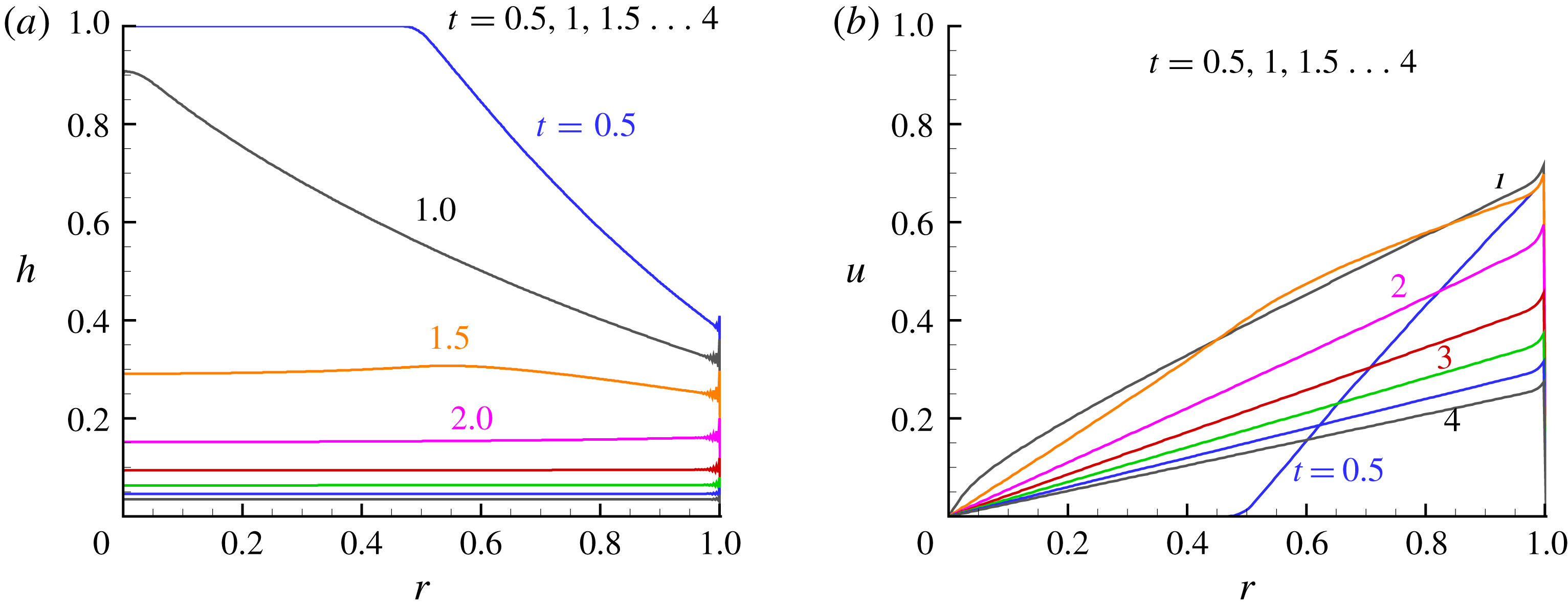
Results are shown in figure 2. Qualitatively, the resulting flow is simple. The dam break of the outer boundary (
 $r=1$
) generates a pressure decrease wave (
 $c_{-}$
characteristic) that is propagated inward as a decrease of
 $h$
(the radial pressure gradient is
 $\propto -\unicode[STIX]{x2202}h/\unicode[STIX]{x2202}r$
). This is accompanied by the appearance of a radial motion (a positive
 $u$
) in the domain activated by that pressure gradient. At
 $t=1$
(approximately) all the fluid in the reservoir is in motion, and the inclination of the interface decays. Subsequently (
 $t>2$
) the interface is nearly flat and
 $u$
is linear with
 $r$
. The fluid is squeezed out of the reservoir as between two disks.
The quantitative details are given by the finite-difference solution in figure 2. We observe some wiggles at
 $r\approx 1$
, which is a spurious by-product of the truncation errors (numerical diffusion and dispersion, see Morton & Mayers (Reference Morton and Mayers1994)), and has negligible influence on the accuracy of the solution at other points, as confirmed later in § 2.2.
SW finite-difference results. (a)
 $h(r,t)$
and (b)
 $u(r,t)$
at
 $t=0.5,1,1.5\ldots 4$
.
2.1.2 Similarity solution
Inspection of the finite-difference profiles of
 $h(r,t)$
and
 $u(r,t)$
suggest that, for large
 $t$
, these variables obey a self-similar behaviour of the type
 ${\sim}t^{-p}f(r)$
. Using the governing equations (2.5) and boundary conditions we find that a solution of this type must satisfy
 $$\begin{eqnarray}h(r,t)=(t+\unicode[STIX]{x1D6FE})^{-2}{\mathcal{H}}(r),\quad u(r,t)=(t+\unicode[STIX]{x1D6FE})^{-1}{\mathcal{U}}(r),\end{eqnarray}$$
where the functions
 ${\mathcal{H}}(r),{\mathcal{U}}(r)$
are determined by the reduced form of the continuity and momentum equations
 $$\begin{eqnarray}-2{\mathcal{H}}+({\mathcal{U}}{\mathcal{H}})^{\prime }=-{\mathcal{H}}{\mathcal{U}}/r,\quad -{\mathcal{U}}+{\mathcal{U}}{\mathcal{U}}^{\prime }+{\mathcal{H}}^{\prime }=0,\end{eqnarray}$$
subject to the boundary conditions
 ${\mathcal{U}}(0)=0$
and
 ${\mathcal{U}}(1)=[{\mathcal{H}}(1)]^{1/2}$
. Here the prime denotes derivative with respect to
 $r$
. The constant
 $\unicode[STIX]{x1D6FE}$
can be estimated by matching the similarity prediction to the finite-difference solution of the SW dam-break problem at some non-small time
 $t_{1}$
.
Surprisingly, an analytical solution exists:
 ${\mathcal{H}}=1,{\mathcal{U}}=r$
. This flow field satisfies the equations (2.9) and the boundary conditions. We observe that the finite-difference solution in figure 2(a) displays a nearly flat interface for
 $t\gtrsim t_{1}\approx 2$
. Matching the numerical mid-reservoir
 $h=0.1536$
at
 $t_{1}=2$
with the similarity solution we obtain
 $\unicode[STIX]{x1D6FE}=0.559$
. The comparison of the
 $h$
and
 $u$
solutions for the subsequent flow is shown in figure 3(a,b).
Comparison of finite-difference solution (solid line) with the similarity solution with
 $\unicode[STIX]{x1D6FE}=0.559$
(dash-dot line); (a)
 $h(r,t)$
at various
 $t$
; (b)
 $u(r,t)$
at various
 $t$
; (c) volume decay
 ${\mathcal{V}}(t)/{\mathcal{V}}(0)$
versus
 $t$
.

2.1.3 Volume decay
The volume
 ${\mathcal{V}}(t)$
is straightforwardly calculated from the finite-difference solution, either by the integral of
 $h(r,t)r\,\text{d}r$
over
 $[0,1]$
, or by using the integral of the outflux
 $u(1,t)h(1,t)\,\text{d}t$
over
 $[0,t]$
. The agreement between the methods is very good (the discrepancy increases with time due to accumulation of errors).
The value of
 ${\mathcal{V}}(t)/{\mathcal{V}}(0)$
decreases rapidly to 0.72 at
 $t=1$
and 0.16 at
 $t=2$
. For larger
 $t$
it is convenient to use the self-similar solution, which gives
 ${\mathcal{V}}(t)/{\mathcal{V}}(0)=(t+\unicode[STIX]{x1D6FE})^{-2}=(t+0.559)^{-2}$
. Comparing with the results of Momen et al. (Reference Momen, Zheng, Bou-Zeid and Stone2017) we note that the major difference between the rectangular and cylindrical reservoir is during the initial ‘slumping’ phase,
 $t\leqslant 2$
. The former reservoir contains
 $0.41{\mathcal{V}}(0)$
at
 $t=2$
. This is a result of the geometry: in the initial stage, the height of the interface decreases first near the edge. In the cylinder the volume is distributed like
 $r^{2}$
, while in the rectangle like
 $x$
(the distance from the back wall). At larger times,
 $t>2$
, in both reservoirs the volume decays like
 $t^{-2}$
.
The similarity solution overestimates the volume left in the reservoir, but the drainage is fairly well captured. For example, the finite-difference solution predicts that at
 $t=5$
, 98 % drainage has been achieved, while similarity gives
 $97\,\%$
. We keep in mind that this result uses the value of
 $\unicode[STIX]{x1D6FE}$
fitted to the finite-difference solution.
2.1.4 Transition to the viscous regime
The formal criterion for the validity of the SW formulation is
 $Re=(g^{\prime }h_{0})^{1/2}h_{0}/\unicode[STIX]{x1D708}\gg 1$
. During the process the speed and thickness decrease, and hence the ratio of inertia to viscous forces decreases. A more stringent criterion is needed, the time dependent effective Reynolds number,
 $Re_{e}=Re_{e}(t)$
.
We make the following estimate. Let
 $u^{\ast }(r_{0},t)$
and
 $h^{\ast }(r_{0},t)$
be the dimensional values at the edge. The inertia per unit volume is
 $\unicode[STIX]{x1D70C}_{1}[u^{\ast }(r_{0},t)]^{2}/r_{0}$
, while the viscous force per unit bottom area is
 $\unicode[STIX]{x1D70C}_{1}\unicode[STIX]{x1D708}[u^{\ast }(r_{0},t)]/h^{\ast }(r_{0},t)$
. The integral over the dense fluid then gives the ratio of inertial to viscous effects as
 $$\begin{eqnarray}Re_{e}=\frac{u^{\ast }(r_{0},t)[h^{\ast }(r_{0},t)]^{2}}{\unicode[STIX]{x1D708}r_{0}}.\end{eqnarray}$$
Switching to the dimensionless
 $u$
and
 $h$
yields
 $$\begin{eqnarray}Re_{e}=\left[Re\frac{h_{0}}{r_{0}}\right]u(r=1,t)[h(r=1,t)]^{2}=\left[Re\frac{h_{0}}{r_{0}}\right]\unicode[STIX]{x1D6E4}(t),\end{eqnarray}$$
where
 $\unicode[STIX]{x1D6E4}$
is of the order of unity at the beginning of the process, but decreases with time. Eventually, the SW inertial–buoyancy flow is expected to undergo transition to a viscous–buoyancy regime when
 $Re_{e}\approx 1$
.
 $\unicode[STIX]{x1D6E4}$
can be calculated from the finite-difference solution, and for
 $t\geqslant 2$
we can use the similarity solution and find
 $\unicode[STIX]{x1D6E4}\approx (t+\unicode[STIX]{x1D6FE})^{-5}$
. Thus, even for a moderately large
 $Reh_{0}/r_{0}\gtrsim 10^{3}$
, a very significant inertial draining is expected to occur for approximately 4–5 time units, during which the volume decays to less than
 $5\,\%$
of
 ${\mathcal{V}}(0)$
.
2.2 Comparison to direct numerical Navier–Stokes simulations
For assessing the reliability of the predictions of the simplified SW model it is necessary to perform comparisons with realistic ‘experimental’ data. Here we use a numerical simulation of the Navier–Stokes equations for the two-fluid configuration. In the Momen et al. (Reference Momen, Zheng, Bou-Zeid and Stone2017) investigation of the 2-D reservoir, both laboratory experiments and DNS have been used. There was excellent agreement between the data used for comparison with the SW model, and actually the DNS data turned out to be more reliable and flexible for processing for the task of comparison. Based on this evidence, we decided to compare the predictions of the model with DNS data of the type used by Momen et al. (Reference Momen, Zheng, Bou-Zeid and Stone2017). We proceed as follows.
We use an open-source toolbox OpenFOAM® (Weller et al. Reference Weller, Tabor, Jasak and Fureby1998) to conduct DNSs for the two-phase flow problem. We solve the incompressible, isothermal Navier–Stokes equations by using the ‘interIsoFoam’ solver (an extension of OpenFOAM), equipped with a novel volume-of-fluid (VOF) method ‘isoAdvector’ (Roenby, Bredmose & Jasak Reference Roenby, Bredmose and Jasak2016) to capture and advect the interfaces between the two phases.
Following Momen et al. (Reference Momen, Zheng, Bou-Zeid and Stone2017), we perform simulations for a realistic, axisymmetric configuration, where we choose water of density
 $\unicode[STIX]{x1D70C}_{1}=998\text{ kg }\text{m}^{-3}$
and air of density
 $\unicode[STIX]{x1D70C}_{2}=1.2\text{ kg }\text{m}^{-3}$
as the two fluids. The kinematic viscosities are
 $\unicode[STIX]{x1D708}_{1}=10^{-6}\text{ m}^{2}\text{ s}^{-1}$
, and
 $\unicode[STIX]{x1D708}_{2}=1.5\times 10^{-5}\text{ m}^{2}\text{ s}^{-1}$
, respectively. To stabilize the simulations, we also use a realistic surface tension coefficient of
 $0.07\text{ N }\text{m}^{-1}$
. At time zero, fluid in the cylindrical reservoir is of radius
 $r_{0}=0.2\text{ m}$
and height
 $h_{0}=0.02\text{ m}$
(see figure 4). A solid domain of height
 $h_{\text{s}}=0.04\text{ m}$
is imposed beneath the reservoir such that its bottom satisfies a no-slip boundary condition. The reservoir and its solid support are embedded in a much larger box-like computational domain, which contains the ‘ambient’ fluid, similar to that of Momen et al. (Reference Momen, Zheng, Bou-Zeid and Stone2017). The boundary conditions imposed on the large ambient are: no slip at the bottom and lateral sides of the domain, and a constant pressure at its top. The size of this entire computational domain is
 $r\in [0,4]\text{m}$
and
 $z\in [-2,2]\text{m}$
, much larger than the size of the reservoir, and hence the DNS mimics an ‘unbounded’ ambient fluid. The switch to dimensionless variables, using (1.1)–(2.4), is straightforward. For generality and a convenient comparison with the theory, hereafter the DNS variables and results will be reported in dimensionless form.
We note that the simulated system provides good compatibility with the assumptions of the SW model: the ratio
 $h_{0}/r_{0}=0.1$
is small, the formal
 $Re=(g^{\prime }h_{0})^{1/2}h_{0}/\unicode[STIX]{x1D708}_{1}=8.9\times 10^{3}$
is large and the flow in the large ambient is expected to be weak because the dimensionless computational domain is
 $r\in [0,40],z\in [-100,100]$
.
We use a grid resolution of
 $\unicode[STIX]{x0394}r=5\times 10^{-4},\unicode[STIX]{x0394}z=5\times 10^{-3}$
, which seems to be sufficient as indicated a posteriori by the satisfactory comparison between the numerical and theoretical results. It it noteworthy that to build an axisymmetric set-up in OpenFOAM, a wedge-shaped Cartesian grid (see the inset of figure 4) is required, where we adopt a wedge angle of
 $0.5^{\circ }$
and one cell layer distribution in the azimuthal direction. The ‘wedge’ boundary conditions need to be specified at the two vertical planes.
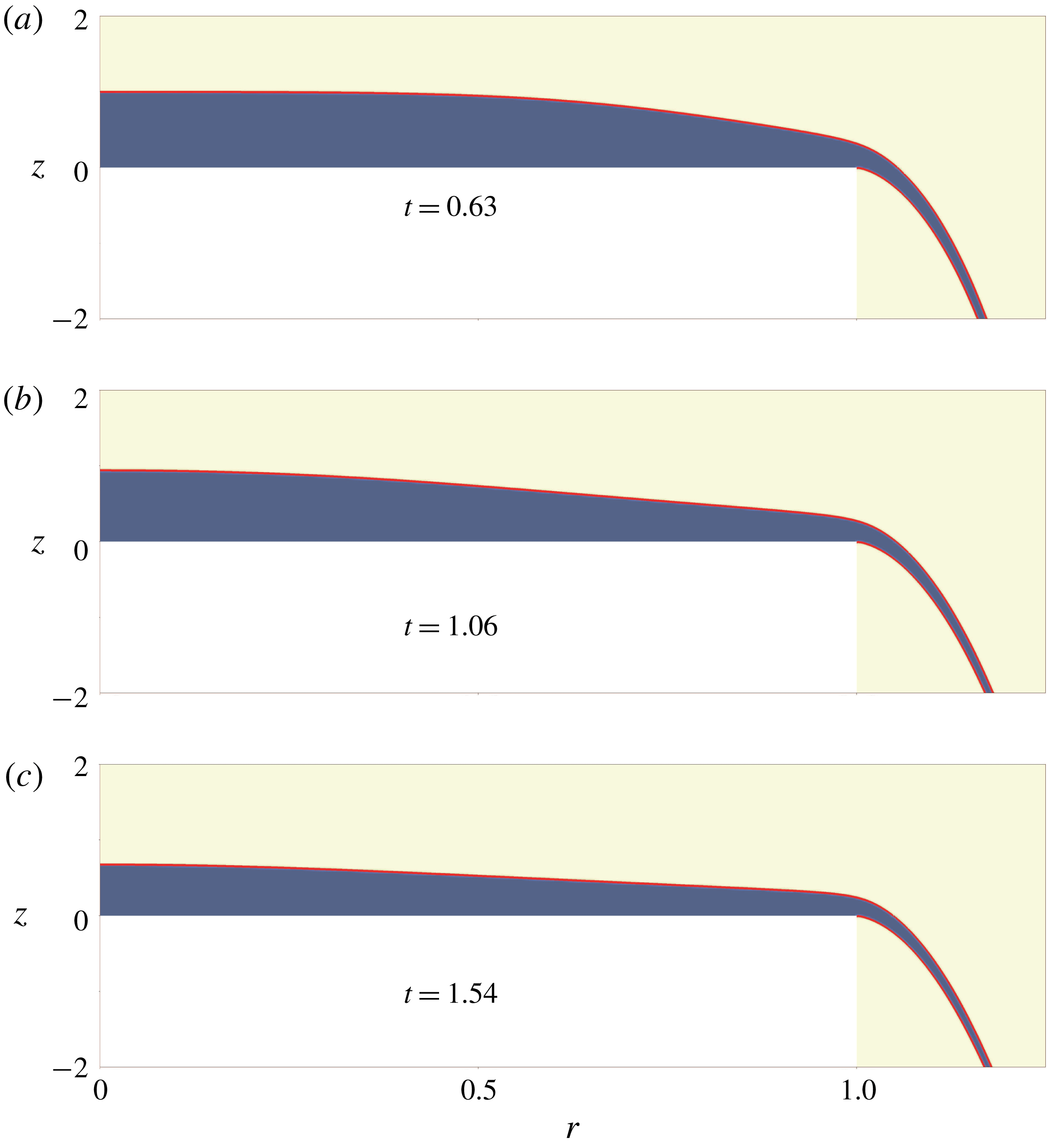
We use an open-source visualization tool of Childs et al. (Reference Childs2012) to analyse the DNS data. As shown in figure 5, we extract the contour level,
 $0.5$
, of the volume fraction representing the interface (red curves) between the two phases. Based on the extracted profile
 $h(r,t)$
with
 $r\in [0,1]$
, we compute the volume
 $V(r,t)=2\unicode[STIX]{x03C0}\int _{0}^{r}sh(s,t)\,\text{d}s$
of the remaining water inside a cylindrical domain of radius
 $r$
in the reservoir. The depth-averaged velocity
 $u(r,t)$
can be calculated by
 $$\begin{eqnarray}u(r,t)=-\frac{1}{2\unicode[STIX]{x03C0}rh}\frac{\text{d}V}{\text{d}t}.\end{eqnarray}$$
As expected, this velocity agrees well with that obtained by directly depth integrating the horizontal velocity field of the DNS at the radial position
 $r$
. One single case of the simulations required approximately two days based on two nodes (each is equipped with an Intel Xeon E5-2690v4 CPU) of the Kebnekaise cluster of HPC2N at Umeå University.
DNS approach: sketch of the three-dimensional axisymmetric numerical configuration. The blue area denotes the cylindrical reservoir of radius
 $r_{0}$
and height
 $h_{0}$
at time zero, and the black area indicates a solid domain of height
 $h_{s}$
. The inset shows the wedge-shaped Cartesian grid required by OpenFOAM for an axisymmetric set-up.


Comparison of DNS and SW results for outward drainage: (a)
 $h(r,t)$
; (b)
 $u(r,t)$
at
 $t=1,2,3,4$
; and (c)
 ${\mathcal{V}}(t)/{\mathcal{V}}(0)$
versus
 $t$
.

2.2.1 Results
The comparisons for the height and velocity (
 $z$
-averaged) profiles
 $h(r,t)$
and
 $u(r,t)$
at various
 $t$
are shown in figure 6(a,b). Overall, there is very good agreement for both variables. At the outflow edge
 $r\approx 1$
we observe a discrepancy between the model and the data. We must keep in mind that
 $r\approx 1$
is a sub-domain of the complex flow, which defies simple modelling. The drained fluid turns over a sharp edge, and local acceleration and vorticity terms are expected to influence the dynamics. The SW model is based on
 $z$
-averaged inviscid balances that are bound to miss these local, strongly
 $z$
-dependent, effects. Therefore, the discrepancy in the edge domain should be considered as an expected feature of the model: loss of accuracy of the averaged variables in a region of a sharp change of flow conditions.
The important variable of the reservoir flow is the volume decay, for which the comparison is shown in figure 6(c). The comparison is shown until
 $t=6$
at which
 $99\,\%$
of
 ${\mathcal{V}}(0)$
has been drained out. The agreement is very good for the entire period of time: the difference between the SW and the DNS volume predictions is smaller than
 $0.5\,\%$
of
 ${\mathcal{V}}(0)$
. This demonstrates that the averaging method used for the SW model is actually more robust than could be inferred from figure 6(a,b). The edge discrepancies of
 $u$
and
 $h$
compensate each other, and the net outflow
 $uh$
is accurate (as compared to the DNS data). We could not find any analytical justification of this behaviour (i.e. robust/accurate
 $uh$
in spite of discrepancies and wiggles in
 $u$
and
 $h$
). In any case, the comparisons presented in figure 6 provide strong support to the predictive power of the SW model with the critical height-averaged outflux condition (2.7) for the reservoir-drainage problem, for the entire period of practical interest.
3 Inward drainage
In this section we consider that the projection of the reservoir is an annulus
 $r\in [r_{i},1]$
(scaled with the outer radius
 $r_{0}$
), and the initial height is 1 (scaled with
 $h_{0}$
). The dam break occurs at the inner wall, and we expect a negative
 $u$
. The scaling of velocity, height, radius and time is as before, see (2.3). Here it is also convenient to use the time
 $\tilde{t}$
scaled with the reference time
 $\tilde{T}=(r_{0}-r_{i})/U$
. The interpretation is that the gap
 $r_{0}-r_{i}$
is the relevant distance for the propagation of the fluid (and of the characteristics). The conversion is
 $\tilde{t}=t/(1-r_{i})$
.
Assuming that the ratio of gap
 $r_{0}-r_{i}$
to height
 $h_{0}$
is large, and
 $Re\gg 1$
, we can apply the SW simplifications for the domain
 $r\in [r_{i},1]$
. The SW equations of motion (2.5), and the corresponding characteristics (2.6), are valid, and the initial conditions are again
 $h=1,u=0$
. The boundary conditions are now:
 $u(r=1,t)=0$
and
 $u(r_{i},t)=-[h(r_{i},t)]^{1/2}$
. The flow is converging, from the periphery to the centre.
The finite-difference method used for the full cylinder is straightforwardly applied to this problem. Figure 7 displays results for the behaviour of
 ${\mathcal{V}}(\tilde{t})/{\mathcal{V}}(0)$
for various
 $r_{i}$
, and the results for a rectangle of length
 $r_{0}-r_{i}$
(see appendix A) are also shown. We observe that for
 $r_{i}=0.9$
the flow is as in the rectangular reservoir, because the effect of the curvature terms is small when
 $(r_{0}-r_{i})/r_{0}$
is small. As
 $r_{i}$
decreases, the rate of drainage is reduced. The interpretation is mostly geometrical: the outflux
 $q=r_{i}u_{i}h_{i}$
is restricted by the value of
 $r_{i}$
.
Inward drainage,
 ${\mathcal{V}}/{\mathcal{V}}(0)$
at a function of time
 $\tilde{t}$
for various
 $r_{i}$
. Also shown is the rectangular case (dash line).

Inward drainage,
 $r_{i}=0.5$
: (a)
 $h(r,t)$
and
 $-u(r,t)$
profiles versus
 $r$
at various
 $\tilde{t}$
.

Inward drainage,
 $r_{i}=0.1$
: (a)
 $h$
and (b)
 $-u(r,t)$
profiles versus
 $r$
at various
 $\tilde{t}$
.
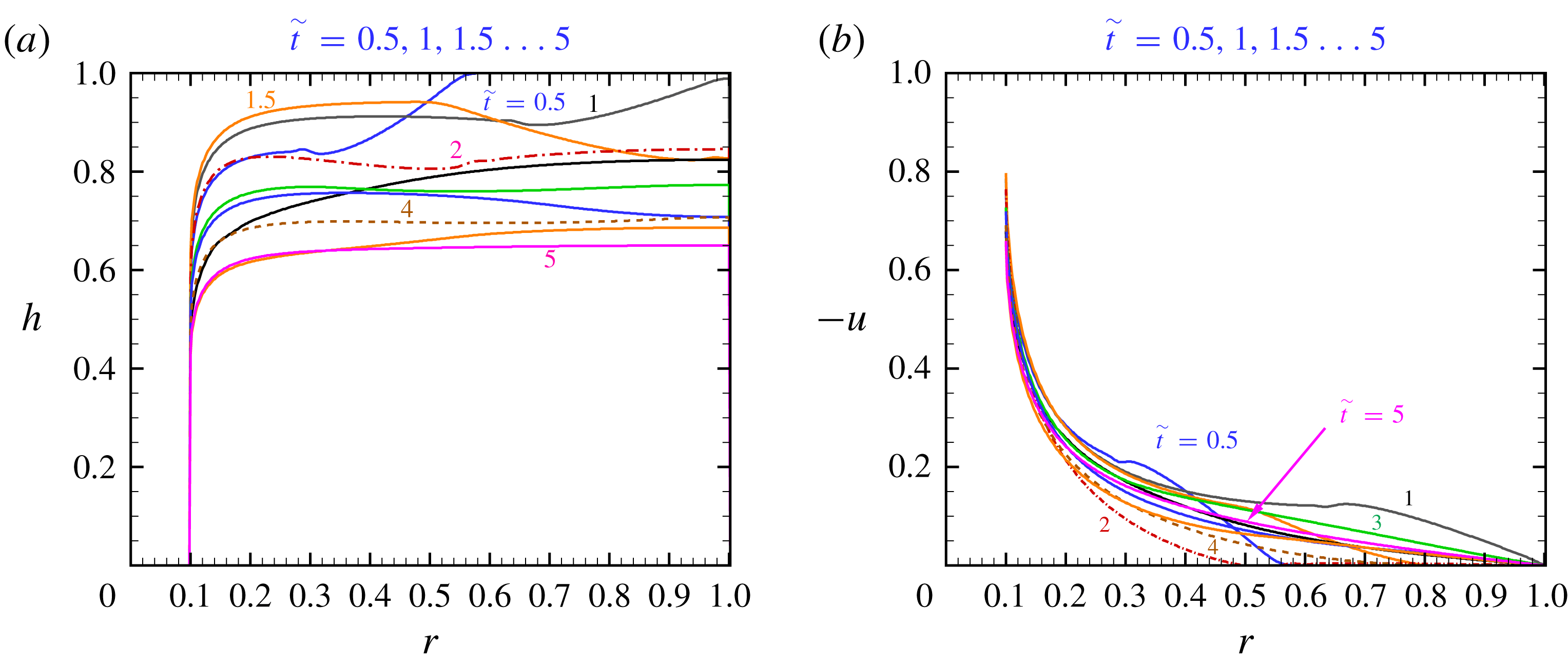
The profiles of
 $h$
and
 $u$
for
 $r_{i}=0.5$
and
 $0.1$
are shown in figures 8 and 9. Typically, the interface is higher in the bulk of the fluid, and lower at
 $r_{i}$
. A wave shape appears during the initial stage (
 $\tilde{t}\approx 1.5$
), then a monotonic decrease with
 $1-r$
prevails. We note that
 $-u$
increases fairly linearly with the distance from the outer boundary
 $1-r$
in the main reservoir, but has a sharp increase as
 $r-r_{i}\rightarrow 0^{+}$
.
3.1 Similarity
Inspection of the finite-difference solutions suggests that the flow tends to a self-similar behaviour for large
 $t$
. Actually, the similarity formulation (2.8)–(2.9) applies to the present problem for
 $r\in [r_{i},1]$
, while the inward flow imposes the boundary conditions
 ${\mathcal{U}}(1)=0$
and
 ${\mathcal{U}}(r_{i})=-[{\mathcal{H}}(r_{i})]^{1/2}$
. We could not find a simple analytical solution, and hence we provide a numerical calculation of the functions
 ${\mathcal{H}}(r)$
and
 ${\mathcal{U}}(r)$
.
For the numerical solution, we first rewrite the system (2.9) in the form
 $$\begin{eqnarray}\displaystyle & \displaystyle {\mathcal{U}}^{\prime }=\frac{1-{\mathcal{U}}/r}{1-{\mathcal{U}}^{2}/{\mathcal{H}}}+1, & \displaystyle\end{eqnarray}$$
 $$\begin{eqnarray}\displaystyle & \displaystyle {\mathcal{H}}^{\prime }={\mathcal{U}}(1-{\mathcal{U}}^{\prime })=-{\mathcal{U}}\frac{1-{\mathcal{U}}/r}{1-{\mathcal{U}}^{2}/{\mathcal{H}}}. & \displaystyle\end{eqnarray}$$
A continuous solution requires
 ${\mathcal{U}}^{2}/{\mathcal{H}}<1$
over the gap
 $(r_{i},1]$
. The boundary condition
 ${\mathcal{U}}(r_{i})=-[{\mathcal{H}}(r_{i})]^{1/2}$
introduces a singularity of the derivatives at
 $r_{i}$
. Using an expansion about this point, we find that the leading-order behaviour for
 $(r-r_{i})\rightarrow 0$
is
 $$\begin{eqnarray}{\mathcal{H}}(r)={\mathcal{H}}_{i}+{\mathcal{H}}_{i}^{1/2}C(r-r_{i})^{1/2},\quad {\mathcal{U}}(r)=-{\mathcal{H}}_{i}^{1/2}+C(r-r_{i})^{1/2},\end{eqnarray}$$
where
 ${\mathcal{H}}_{i}={\mathcal{H}}(r_{i})$
and
 $C=(2/3)^{1/2}{\mathcal{H}}_{i}^{1/4}(1+{\mathcal{H}}_{i}^{1/2}/r_{i})^{1/2}$
(the error is
 $O(r-r_{i})$
). (It is apparently strange that the outward drainage has no such singularity. This is because in the outward case the curvature term
 ${\mathcal{U}}/r$
is positive, and the
 $1-{\mathcal{U}}/r$
numerator in (3.1)–(3.2) can vanish, while for the inward case
 ${\mathcal{U}}/r$
is negative and
 $1-{\mathcal{U}}/r>1$
. Note that in the definition of the coefficient
 $C$
the term
 $1+{\mathcal{H}}^{1/2}/r_{i}$
stands for
 $1-{\mathcal{U}}_{i}/r_{i}$
, and this is
 ${>}1$
for an inward flow with
 ${\mathcal{U}}<0$
. On the other hand, in the outward flow solution,
 ${\mathcal{U}}_{i}/r_{i}=1$
and hence the coefficient
 $C$
vanishes.) The solution is attained by a shooting method: using
 ${\mathcal{U}}(1)=0$
and a guessed
 ${\mathcal{H}}(1)$
, we integrate (3.1)–(3.2) from
 $r=1$
to
 $r_{i}+\unicode[STIX]{x1D6E5}$
, where
 $\unicode[STIX]{x1D6E5}$
is a small interval, i.e.
 $10^{-3}(1-r_{i})$
. Combining with (3.3), we check the fulfilment of the boundary condition
 $-{\mathcal{U}}(r_{i})/[{\mathcal{H}}(r_{i})]^{1/2}=1$
; the guess
 ${\mathcal{H}}(1)$
is corrected as necessary. This method has been applied for various
 $r_{i}$
, and we found convergence in all tested cases. In general,
 ${\mathcal{H}}(1)$
increases strongly as
 $r_{i}$
decreases. On the other hand, the more significant value
 ${\mathcal{H}}(r_{i})/{\mathcal{H}}(1)$
is quite robust: it decreases from
 $0.75$
to 0.
 $69$
as
 $r_{i}$
decreases from
 $0.99$
to
 $0.1$
. Typical values are given in table 1; the typical profiles are displayed in figure 10.
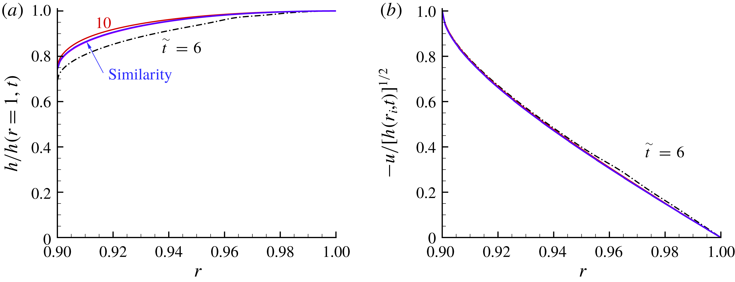
The similarity solution is validated by comparison with the finite-difference solution of the SW equations. Figure 10 shows that the profiles of
 $h(r,t)/h(1,t)$
and
 $u(r,t)/h^{1/2}(r_{i},t)$
approach the similarity curves
 ${\mathcal{H}}(r)/{\mathcal{H}}(1)$
and
 ${\mathcal{U}}(r)/{\mathcal{H}}^{1/2}(r_{i})$
for large
 $t$
. Figure 10 is for a system with
 $r_{i}=0.9$
, and we emphasize that tests with other systems, not shown here, reveal the same pattern. This confirms the spatial behaviour.
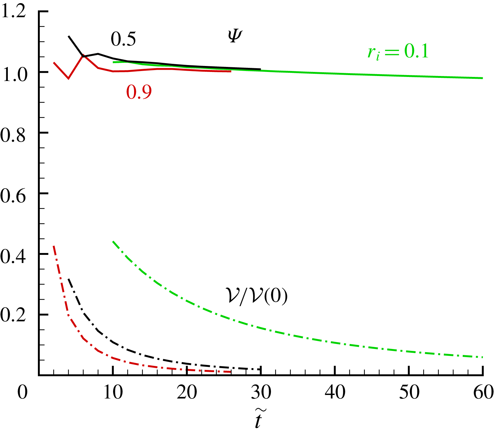
The time-dependent similarity is tested in figure 11. Here we use the SW results
 $h(1,t)$
. We see that
 $h(1,t)(t+\unicode[STIX]{x1D6FE})^{2}$
is close to a constant
 $C$
for a significant span of time (roughly, while
 ${\mathcal{V}}(t)/{\mathcal{V}}(0)$
decreases from 0.4 to 0.01). The value of
 $\unicode[STIX]{x1D6FE}$
is fitted. The results of figure 11 confirm the time dependency predicted by the similarity solution.
Consequently, a good approximation for the volume in the reservoir is
 $$\begin{eqnarray}\frac{{\mathcal{V}}(t)}{{\mathcal{V}}(0)}=K{\mathcal{H}}(1)(t+\unicode[STIX]{x1D6FE})^{-2},\quad K=\frac{2}{{\mathcal{H}}(1)(1-r_{i}^{2})}\int _{r_{i}}^{1}{\mathcal{H}}(r)r\,\text{d}r.\end{eqnarray}$$
The value of
 $K=K(r_{i})$
is calculated numerically (as a simple extension of the solution for
 ${\mathcal{H}}(r),{\mathcal{U}}(r)$
), and typical values are given in table 1. Note that these values are close to
 $1$
. Comparisons of the result (3.4) with SW calculations (not shown here) display good agreement for large
 $t$
, as expected.
Inward drainage,
 $r_{i}=0.9$
: (a)
 $h(r,t)/h(r=1,t)$
versus
 $r$
, and (b)
 $-u(r,t)/[h(r_{i},t)]^{1/2}$
versus
 $r$
, at various
 $\tilde{t}=6,10,20$
. The similarity solution (blue solid line) is also shown. The similarity curve and
 $\tilde{t}=20$
finite-difference line coincide.
Values of the self-similar radial profile, obtained by numerical solution of the reduced system, and
 $\unicode[STIX]{x1D6FE}$
from finite-difference SW solution.

We observe in table 1 that the numerical values of
 ${\mathcal{H}}(1)$
increase sharply as
 $r_{i}$
decreases. We verified that this is a mathematical result of the self-similar formulation, and does not imply a physical behaviour. In the physical variable
 $h$
, the large values of
 ${\mathcal{H}}(1)$
are counteracted by the virtual-origin ingredient of the similarity solution. It turns out that the value
 ${\mathcal{H}}(1)$
is connected with the time
 $t_{m}$
at which the similarity solution becomes relevant (and a matching with the initial-value problem can be performed). We argue as follows:
 ${\mathcal{H}}(1)/(t_{m}+\unicode[STIX]{x1D6FE})^{2}\approx h(1,t_{m})$
. Since during the initial (or slumping) phase of a dam-break flow
 $h(1)>4/9$
, we can estimate that the self-similar flow becomes relevant when
 $h(1,t_{m})\approx 0.5$
, and hence we obtain the estimate
 $$\begin{eqnarray}t_{m}\approx \left[{\textstyle \frac{1}{2}}{\mathcal{H}}(1)\right]^{1/2},\end{eqnarray}$$
which is also given in table 1. The estimate is not sharp, because we have omitted the unknown virtual-origin coefficient
 $\unicode[STIX]{x1D6FE}$
. However, we argue that
 $\unicode[STIX]{x1D6FE}<t_{m}$
, and hence (3.5) remains a useful estimate. Some care is needed in the interpretation of
 $t_{m}$
when
 $r_{i}$
is close to 1 (e.g. 0.9). In these cases
 $t_{m}$
is small, but
 $\tilde{t}_{m}=t_{m}/(1-r_{i})$
is typically
 $4$
. This behaviour could be expected from the 2-D analysis of Momen et al. (Reference Momen, Zheng, Bou-Zeid and Stone2017). Comparisons with the finite-difference solution show that (3.5) captures well the trend. For example, in figure 10 for
 $r_{i}=0.9$
, we see that at
 $\tilde{t}=6$
there is good agreement for both
 $h$
and
 $u$
variables, and for
 $t\geqslant 10$
the finite-difference and similarity curves almost coincide. The same behaviour has been found for other values of
 $r_{i}$
, not shown here.
Inward drainage,
 $\unicode[STIX]{x1D6F9}(t)=h(r=1,t)(t+\unicode[STIX]{x1D6FE})^{2}/{\mathcal{H}}(1)$
(solid line) and
 ${\mathcal{V}}(t)/{\mathcal{V}}(0)$
versus
 $\tilde{t}=t/(1-r_{i})$
for
 $r_{i}=0.1,0.5,$
and
 $0.9$
. The values of
 ${\mathcal{H}}(1)$
and
 $\unicode[STIX]{x1D6FE}$
are given in table 1.
The transition to the viscous regime is estimated with the same arguments as used in § 2.1.4. We find that it is necessary to replace
 $r_{0}$
by the gap
 $r_{0}-r_{i}$
in the definitions (2.10) and (2.11). Upon this change, the same conclusions follow.
3.2 Comparison to DNS
DNS was performed for the inward-drainage problem, for two cases:
 $r_{i}=0.1$
and
 $r_{i}=0.5$
. The details of the numerical approach are similar to § 2.2, and will not be repeated here.
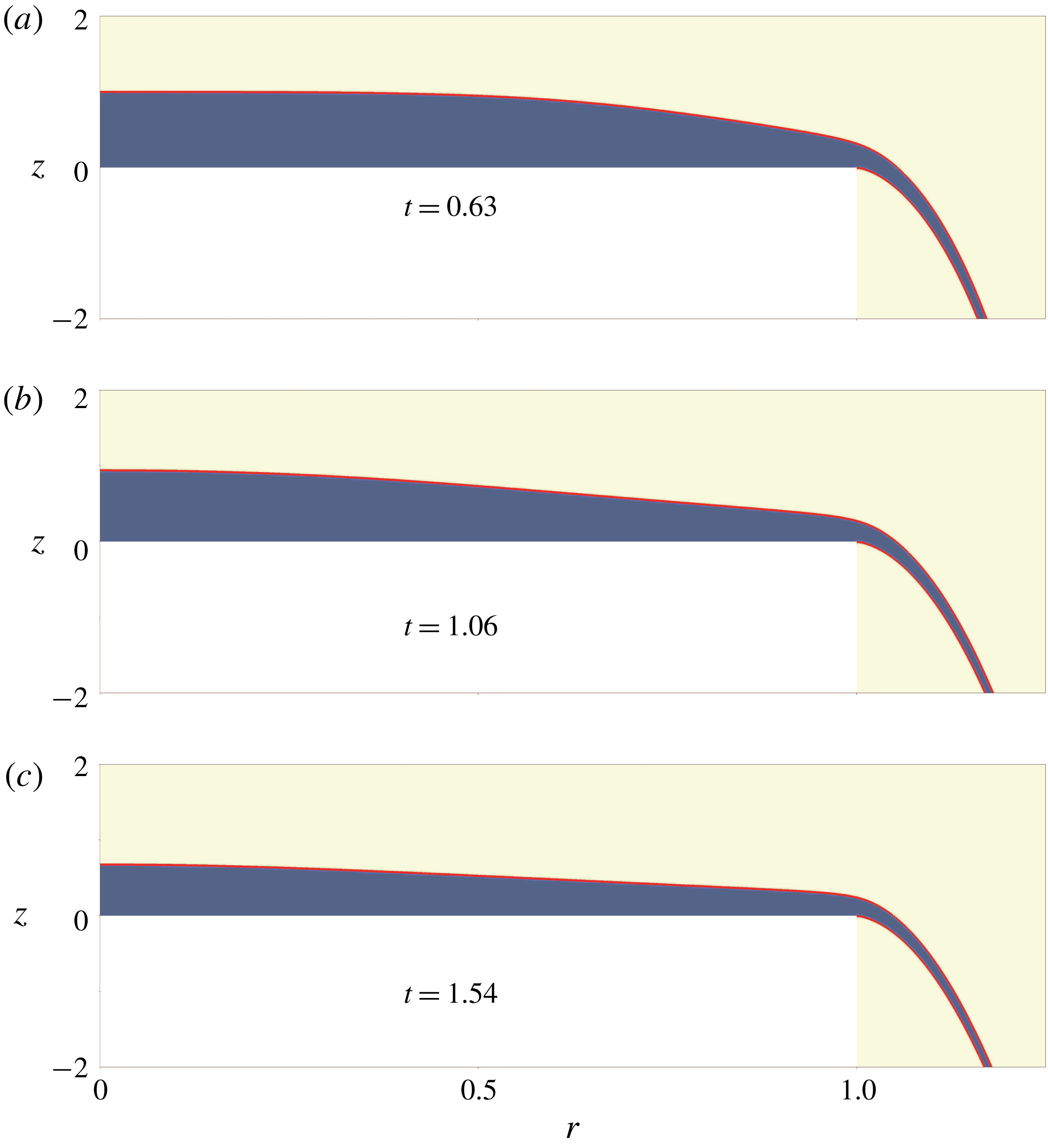
Inward drainage
 $r_{i}=0.5$
. DNS interfacial profiles at dimensionless time (a)
 $\tilde{t}=0.76$
, (b)
 $\tilde{t}=1.64$
and (c)
 $\tilde{t}=3.96$
, where the red curves represent the water–air interfaces. Here
 $r,z$
and
 $\tilde{t}$
are dimensionless.

Comparison of DNS and SW results for inward drainage
 $r_{i}=0.1$
(a)
 $h(r,t)$
, (b)
 $u(r,t)$
at
 $\tilde{t}=1,3,5$
; and (c)
 ${\mathcal{V}}(\tilde{t})/{\mathcal{V}}(0)$
versus
 $\tilde{t}$
.

See previous caption, here for
 $r_{i}=0.5$
.

Snapshots of the DNS position of the dense fluid at various times are displayed in figure 12, for
 $r_{i}=0.5$
. We observe that the interface is inclined toward the edge. With time, the height decreases and the inclination becomes milder.
The comparisons for the height, velocity (
 $z$
-averaged) and volume results are shown in figures 13 and 14, for two values of the inner radius
 $r_{i}$
. Overall, there is fair-to-good agreement. The radial velocity
 $u(r,t)$
has a large slope for
 $r\approx r_{i}$
. The realistic flow in such a domain is expected to contain axial acceleration, and hence some deviation from the hydrostatic balance used in the SW model. This explains the discrepancies between the SW and DNS predictions observed in the figures, in particular concerning the variable
 $u$
, and the behaviour of
 $h$
at early times. Nevertheless, the SW analysis provides the correct scalings of the flow and the influence of
 $r_{i}$
, and predicts well the trends of the variables with
 $r$
and time, and in particular the decay of
 ${\mathcal{V}}(\tilde{t})/{\mathcal{V}}(0)$
.
4 Concluding remarks
We investigated the drainage flow in a cylindrical reservoir in the inertial–buoyancy regime (large Reynolds number), from an initial stationary state, starting with the removal of the curved side boundary. The driving force is the buoyancy represented by the reduced gravity
 $g^{\prime }$
. We show that this flow bears similarities with a gravity current released from a lock (dam break), and can be modelled with the same set of shallow-water (SW) PDE equations for the thickness
 $h$
and radial height-averaged speed
 $u$
as functions of
 $r$
and
 $t$
. However, there is an essential difference in the boundary conditions. We considered two cases of drainage: (i) outward from the outer boundary
 $r_{0}$
in a full-radius reservoir; and (ii) inward from the inner radius
 $r_{i}$
in an annular-shaped reservoir. The boundary condition at the edge is the critical
 $u=(g^{\prime }h)^{1/2}$
at
 $r_{0}$
in case (i), and
 $u=-(g^{\prime }h)^{1/2}$
at
 $r_{i}$
in case (ii). We focused attention in particular on the decay in time of the volume,
 ${\mathcal{V}}(t)/{\mathcal{V}}(0)$
. This work is a consistent extension of the 2-D rectangular reservoir problem studied by Momen et al. (Reference Momen, Zheng, Bou-Zeid and Stone2017). The scales of velocity and time are the same for both geometries. However, the cylindrical geometry introduces significant differences.
Consider case (i). The dimensionless problem has no free input parameters. In particular, the curve
 ${\mathcal{V}}(t)/{\mathcal{V}}(0)$
, where
 $t$
is time scaled with
 $r_{0}/(g^{\prime }h_{0})^{1/2}$
, is universal. The SW equations admit a similarity solution, valid for large
 $t$
(but a fair approximation for
 $t>2$
):
 $h$
decays like
 $t^{-2}$
and
 $u$
decays like
 $t^{-1}$
. The same qualitative long-time behaviour appears in the 2-D reservoir. Surprisingly, the
 $r$
-profile of the similarity solution is simple: flat
 $h$
and linear
 $u$
. This is in strong contrast with the downward curved
 $h$
and upward curved
 $u$
, both with singular slope at the edge, which appear in the 2-D reservoir. The SW model predictions were compared with the DNS solution. The agreement is very good for the
 ${\mathcal{V}}(t)/{\mathcal{V}}(0)$
variable and good for
 $h$
and
 $u$
. This agreement provides strong support to the model used in this study. Also, the outward drainage in the cylindrical geometry is more rapid than in the 2-D counterpart: for example, at
 $t=2$
the value
 ${\mathcal{V}}/{\mathcal{V}}(0)$
is 0.16 in the former and 0.41 in the latter geometry.
Consider case (ii). The reduced problem, and the curve
 ${\mathcal{V}}(t)/{\mathcal{V}}(0)$
, depends on the
 $r_{i}/r_{0}$
input parameters. Both
 $h$
and
 $u$
have
 $(r-r_{i})^{1/2}$
singularities as
 $r\rightarrow r_{i}$
. The SW equations admit a similarity solution, valid for large
 $t$
, and, again,
 $h$
decays like
 $t^{-2}$
,
 $u$
decays like
 $t^{-1}$
. The
 $r$
-dependence of the similarity profiles must be calculated numerically. Again, the SW solution has been corroborated by comparisons with DNS results. When
 $r_{i}/r_{0}$
is small the drainage is slow because of the small
 $r_{i}u_{i}h_{i}$
outflux, the main motion occurs in a small region close to
 $r_{i}$
, while in the bulk of the reservoir (
 $r>2r_{i}$
say) the interface is close to horizontal and the velocity is small. When the gap
 $(r_{0}-r_{i})/r_{0}$
is small, the curvature terms are unimportant and the present SW results are very close to the 2-D SW solution of Momen et al. (Reference Momen, Zheng, Bou-Zeid and Stone2017). This compatibility provides further support to our model, because the 2-D model has been corroborated by both experiments and DNS.
The SW results are valid for both Boussinesq and non-Boussinesq systems. The inertial model is relevant when
 $(g^{\prime }h_{0})^{1/2}h_{0}^{2}/(\unicode[STIX]{x1D708}L)\gg 1$
, where
 $L$
is the gap
 $r_{0}-r_{i}$
. The effective Reynolds number decreases with time, but even for modestly large values of
 $(g^{\prime }h_{0})^{1/2}h_{0}^{2}/(\unicode[STIX]{x1D708}L)\gg 1$
a significant discharge occurs in the inertial domain. Our results provide insight, and a simple quantitative prediction, of the behaviour of the volume
 ${\mathcal{V}}(t)/{\mathcal{V}}(0)$
, which is a major concern in practical reservoir-break problems.
We showed that such fairly complex fluid-dynamical systems are amenable to a reduction to simple analytical models. We followed the method used by Momen et al. (Reference Momen, Zheng, Bou-Zeid and Stone2017). First, we use the SW formulation of a gravity current. This model provides the critical boundary condition at the edge,
 $u=\pm (g^{\prime }h)^{1/2}$
(the sign depends on the out- or inward case). Moreover, this model can be solved by a standard finite-difference method (in insignificant CPU time). Second, we reduce the SW PDE formulation to a self-similar form that requires the solution of ODEs. This reduction is insightful concerning the radial profiles and the time decay. However, this solution is not a self-contained prediction model, because: (i) the self-similar flow becomes valid after some adjustment time,
 $t_{m}$
, during which the PDEs require a numerical solution; (ii) the time dependence of the similarity function includes a virtual-origin shift
 $\unicode[STIX]{x1D6FE}$
, which eludes analytical prediction. We estimated
 $\unicode[STIX]{x1D6FE}$
by fitting to the numerical solution at some intermediate time.
We do not claim that the SW model is a substitute for the DNS of the problem. When small-scale details such as mixing, Kelvin–Helmholtz vortices at the interface, the
 $z$
-profile of the velocity or deviations from axial symmetry are needed, DNSs (or experiments) are unavoidable. However, in many cases an estimate is needed for the global behaviour of the flow in a dam-break case, and for this task the present SW analysis can be recommended.
A serious limitation of the simple SW models is the geometry, two-dimensional or axisymmetric. The dam break is assumed to occur all over the width in the 2-D case, and over the entire curved boundary in the axisymmetric case. This can be modelled by a one-dimensional horizontal coordinate equation. In practical situations, the lateral boundary may collapse in some parts only, and the resulting flow cannot be described by a one-dimensional equation with a critical outflux condition. The available SW models may be helpful for some estimates of the more complex cases. First, we can suggest dividing the tank into wedges by radial walls. Drainage occurs only for the wedge whose wall is damaged, and can be estimated by the present results for
 ${\mathcal{V}}(t)/{\mathcal{V}}(0)$
, with the corresponding
 ${\mathcal{V}}(0)$
. Second, consider a container whose basis is a rectangle of side
 $a$
. If all four boundaries collapse, the fluid will propagate away from the centre, and the full-cylinder axisymmetric approximation is expected to be relevant. We notice in this context that there is evidence from gravity currents that corners become rounded after release (see Simpson (Reference Simpson1997) and Zgheib, Bonometti & Balachandar (Reference Zgheib, Bonometti and Balachandar2015) figures 6.6 and 6.7). Third, when only a sector
 $\unicode[STIX]{x1D6E9}$
of the cylindrical boundary of an axisymmetric tank collapses, the volume decay will be significantly smaller than in the standard case. A box-model estimate for this case is given in appendix B; interestingly, for the half-broken
 $\unicode[STIX]{x1D6E9}=\unicode[STIX]{x03C0}$
case,
 ${\mathcal{V}}(t)/{\mathcal{V}}(0)$
behaves like a 2-D solution. The accurate modelling and clarification of these issues requires a good deal of additional analytical, DNS and experimental research, which must be left for future work. We hope that the present paper will provide motivation and guidelines for the additional progress.
Acknowledgements
M.U. thanks the Department of Mechanical and Aerospace Engineering at Princeton university for supporting a visit in summer 2018 during which a part of this study was performed. L.Z. is grateful for a VR International Postdoc Grant from Swedish Research Council ‘2015-06334’. The computer time was provided by SNIC (Swedish National Infrastructure for Computing). L.Z. and H.A.S. are grateful to the Princeton University Carbon Mitigation Initiative for partial support of this research.
Appendix A. Two-dimensional reservoir
For the convenience of the reader, we present a short summary of the SW 2-D counterpart case, following Momen et al. (Reference Momen, Zheng, Bou-Zeid and Stone2017). The
 $r$
coordinate is replaced by the Cartesian
 $x\in [0,x_{0}]$
, and the height is again
 $h_{0}$
. The scaling is as in (2.3)–(2.4), with
 $r_{0}$
replaced by
 $x_{0}$
. In this case the break of the
 $x=0$
or
 $x=1$
boundary is interchangeable as concerns the drainage process. For definiteness, we consider outflux from
 $x=1$
, and a fixed wall at
 $x=0$
.
The SW equations are (2.5) without the curvature terms
 $$\begin{eqnarray}\left[\begin{array}{@{}c@{}}h_{t}\\ u_{t}\\ \end{array}\right]+\left[\begin{array}{@{}cc@{}}u & h\\ 1 & u\end{array}\right]\left[\begin{array}{@{}c@{}}h_{x}\\ u_{x}\end{array}\right]=\left[\begin{array}{@{}c@{}}0\\ 0\end{array}\right].\end{eqnarray}$$
The system is hyperbolic and the characteristics give
 $$\begin{eqnarray}\text{d}h\pm h^{1/2}\,\text{d}u=0\quad \text{on}\quad \frac{\text{d}x}{\text{d}t}=c_{\pm }=u\pm h^{1/2}.\end{eqnarray}$$
The initial conditions are
 $h=1,u=0$
and the boundary conditions are
 $u(x=0,t)=0$
, and
 $u=h^{1/2}$
at
 $x=1$
.
This system admits an analytical solution for
 $t<1$
. The integration along the characteristics provides analytical connections between
 $u$
and
 $\sqrt{h}$
, which subject to the simple initial conditions yield explicitly
 $h(x,t)$
and
 $u(x,t)$
. This is exactly the dam-break flow in the reservoir, see Ungarish (Reference Ungarish2009). (After the removal of the gate at
 $t=0$
, a current propagates to
 $x>1$
, but this flow is not of interest in the present case.) In particular, along a
 $c_{+}$
characteristic we obtain
 $u=2(1-h^{1/2})$
. Combining with the critical
 $c_{-}=u-h^{1/2}=0$
at
 $x=1$
, we find the at this position the constant
 $h=4/9,u=2/3$
and the outflux
 $q=uh=8/27$
.
A rarefaction wave propagates from
 $x=1$
into the reservoir with speed
 $-1$
; the fluid at
 $x<1-t$
is unperturbed. In the activated region
 $1-t<x<1$
,
 $h$
decreases and
 $u$
increases with
 $x$
. At
 $t=1$
this wave is reflected from the
 $x=0$
wall, and will reach the
 $x=1$
boundary at
 $t=1.8$
. Therefore, until
 $t=1.8$
, the outflux condition
 $q=uh=8/27$
remains valid. It is now evident that
 ${\mathcal{V}}(t)/{\mathcal{V}}(0)=1-(8/27)t$
during this stage, and
 ${\mathcal{V}}(2)/{\mathcal{V}}(0)\approx 0.41$
.
For larger
 $t$
a self-similar behaviour appears. The formulation is close to (2.8)–(2.9), but without the curvature terms, as follows
 $$\begin{eqnarray}h(x,t)=(t+\unicode[STIX]{x1D6FE})^{-2}{\mathcal{H}}(x),\quad u(x,t)=(t+\unicode[STIX]{x1D6FE})^{-1}{\mathcal{U}}(x),\end{eqnarray}$$
where the functions
 ${\mathcal{H}}(x),{\mathcal{U}}(x)$
are determined by the reduced form of the continuity and momentum equations
 $$\begin{eqnarray}-2{\mathcal{H}}+({\mathcal{U}}{\mathcal{H}})^{\prime }=0,\quad -{\mathcal{U}}+{\mathcal{U}}{\mathcal{U}}^{\prime }+{\mathcal{H}}^{\prime }=0,\end{eqnarray}$$
subject to the boundary conditions
 ${\mathcal{U}}(0)=0$
and
 ${\mathcal{U}}(1)=[{\mathcal{H}}(1)]^{1/2}$
. Here the prime denotes derivative with respect to
 $x$
.
Momen et al. (Reference Momen, Zheng, Bou-Zeid and Stone2017) derived the analytical solution. Letting
 $w=w(x)={\mathcal{H}}(x)/{\mathcal{H}}(0)$
, this can be expressed in the implicit form
 $$\begin{eqnarray}\frac{x}{\sqrt{{\mathcal{H}}(0)}}=-\frac{1}{2}\unicode[STIX]{x03C0}+2\sqrt{w(1-w)}+\arctan \sqrt{w/(1-w)},\quad \frac{{\mathcal{U}}(w)}{\sqrt{{\mathcal{H}}(0)}}=2\sqrt{w(1-w)}.\end{eqnarray}$$
The
 $w(x)$
profile decreases from
 $1$
to
 $3/4$
, while
 ${\mathcal{U}}$
increases from
 $0$
to
 ${\mathcal{U}}(1)=\sqrt{{\mathcal{H}}(1)}=2.53$
. Both
 ${\mathcal{H}}$
and
 ${\mathcal{U}}$
have singular derivatives at
 $x=1$
. The outflux (rate of discharge) is
 $q=[2.53/(t+\unicode[STIX]{x1D6FE})]^{3}$
. We match this result at
 $t=1.8$
with the dam-break/slumping phase known solution
 $q=8/27$
, and obtain
 $\unicode[STIX]{x1D6FE}\approx 2.0$
. The finite-difference solution recovers very well these analytical features, and also provides the
 $u(x,t)$
and
 $h(x,t)$
behaviour for
 $t>1$
which is not covered by the simple dam-break results.
The 2-D flow is expected to be a good approximation to the inward draining case with small
 $1-r_{i}$
, where the curvature terms are small (subject to the interpretation that
 $x$
is in the direction
 $-r$
, and the length of the reservoir
 $x_{0}=r_{0}-r_{i}$
(dimensional)). This is illustrated in figure 7 for
 $r_{i}=0.9$
. Also, in table 1, we report the interface height ratio
 ${\mathcal{H}}(r_{i})/{\mathcal{H}}(1)=0.742$
for
 $r_{i}=0.9$
, which is close to the 2-D value
 $3/4$
. In all other cases, and in particular for the outflow from a full cylinder, the presence of the curvature term produces significant differences from the 2-D flow.
Appendix B. Partial-break box model
We consider the outward flow case. The reservoir is a full cylinder, but dam break occurs for only a part of the boundary represented by the sector
 $\unicode[STIX]{x1D6E9}$
. The objective is to estimate
 ${\mathcal{V}}(t)/{\mathcal{V}}(0)$
. We use the scaling (2.3)–(2.4).
The ‘box model’ is an accepted simplified tool of analysis of gravity currents (see Ungarish Reference Ungarish2009). The major assumption is that the interface between the dense and ambient fluid is a simple geometric shape, typically a simple box. The motion of this box is governed by volume continuity and boundary conditions derived from momentum balances, or given by some known jump conditions. This method lacks rigor, and its major justification is the evidence that the parameter dependency of the results is usually consistent with more rigorous results and experimental data.
In the spirit of that method, we argue as follows. The fluid in the reservoir can be represented, approximately, by a cylinder box of height
 $h(t)$
. In the realistic system the dam break will cause inclination of the interface toward the exit. Supposing that the gap is not very wide (
 $\unicode[STIX]{x1D6E9}\leqslant \unicode[STIX]{x03C0}$
say), the average slope over the area is not expected to be large, and hence this approximation makes sense. Consequently, the volume of the fluid in the box, scaled with
 $h_{0}r_{0}^{2}$
is given by
 ${\mathcal{V}}(t)=\unicode[STIX]{x03C0}h(t)$
, and initially
 $h(0)=1$
.
Next, we claim that the outflux is governed by the local behaviour of the characteristics, and hence the
 $u=h^{1/2}$
condition, with the initial
 $h_{I}=4/9$
, can be applied over the broken boundary
 $r=1,0<\unicode[STIX]{x1D703}<\unicode[STIX]{x1D6E9}$
. Therefore the rate of drainage of volume is given by
 $$\begin{eqnarray}q\unicode[STIX]{x1D6E9}=uh\unicode[STIX]{x1D6E9}=\left\{\begin{array}{@{}ll@{}}(4/9)^{3/2}\unicode[STIX]{x1D6E9}\quad & (t\leqslant t_{I})\\ \text{}[h(t)]^{3/2}\unicode[STIX]{x1D6E9}\quad & (t>t_{I}),\end{array}\right.\end{eqnarray}$$
where
 $t_{I}$
is the time at which
 $h(t)$
attains
 $h_{I}=4/9$
.
Finally, we apply the volume conservation
 $\unicode[STIX]{x03C0}(\text{d}h/\text{d}t)=-q\unicode[STIX]{x1D6E9}$
, and integrate. After some algebra we obtain
 $$\begin{eqnarray}h(t)=\frac{{\mathcal{V}}(t)}{{\mathcal{V}}(0)}=\left\{\begin{array}{@{}ll@{}}\displaystyle 1-\frac{\unicode[STIX]{x1D6E9}}{\unicode[STIX]{x03C0}}\frac{8}{27}t\quad & (t\leqslant t_{I})\\ \displaystyle \frac{4}{9}\left[1+\frac{1}{3}\frac{\unicode[STIX]{x1D6E9}}{\unicode[STIX]{x03C0}}(t-t_{I})\right]^{-2}\quad & (t>t_{I})\end{array}\right.\end{eqnarray}$$
and the relationship
 $h(t_{I})=h_{I}=4/9$
yields
 $$\begin{eqnarray}t_{I}=\frac{15}{8}\frac{\unicode[STIX]{x1D6E9}}{\unicode[STIX]{x03C0}}.\end{eqnarray}$$
The qualitative behaviour is a quick initial drainage, followed by a
 ${\sim}t^{-2}$
decay. The agreement with the rigorous SW results is encouraging. Moreover, this simple estimate indicates the effect of the part break via the parameter
 $\unicode[STIX]{x1D6E9}/\unicode[STIX]{x03C0}$
. The rate of drainage in both stages decreases when
 $\unicode[STIX]{x1D6E9}/\unicode[STIX]{x03C0}$
decreases. This could be expected.
It is interesting to consider the half-broken
 $\unicode[STIX]{x1D6E9}/\unicode[STIX]{x03C0}=1$
case. Substitution into the previous solution gives:
 $t_{I}=1.9$
and
 $$\begin{eqnarray}\frac{{\mathcal{V}}(t)}{{\mathcal{V}}(0)}=1-\frac{8}{27}t\quad (t\leqslant 1.9).\end{eqnarray}$$
This is almost identical with the 2-D exact result, see appendix A. In both cases,
 ${\mathcal{V}}(2)/{\mathcal{V}}(0)\approx 0.41$
. The subsequent decay of volume is also very similar.