Introduction
It is important to be able to monitor penguins in the Antarctic to enhance our understanding of Southern Ocean ecology (Trathan et al. Reference Trathan, García-Boroboglu, Boersma, Bost, Crawford, Crossin, Cuthbert, Dann, Davis, de la Puente, Ellenberg, Lynch, Mattern, Putz, Seddon, Trivelpiece and Wienecke2015) and, more generally, as indicators of environmental variability and change (Weimerskirch et al. Reference Weimerskirch, Inchausti, Guinet and Barbraud2003, Boersma Reference Boersma2008, Forcada & Trathan Reference Forcada and Trathan2009). Three of the six penguin species that breed in the Antarctic are Pygoscelis penguins (Croxall & Kirkwood Reference Croxall and Kirkwood1979): Adélie (P. adeliae (Hombron & Jacquinot)), gentoo (P. papua Forster) and chinstrap (P. antarctica Forster). These species are numerous and are key consumers within Southern Ocean foodwebs, in particular of Antarctic krill (Euphausia superba Dana), one of the main prey species also consumed by a broad guild of fish, squid, seabirds and marine mammals. Because of their sensitivity to variation in krill stocks, these penguin species are all considered to be valuable indicators of environmental variability and change, and thus of ecosystem status (Ainley Reference Ainley2002). Indeed, the Commission for the Conservation of Antarctic Marine Living Resources (CCAMLR), which manages fisheries in the Southern Ocean including the fishery for Antarctic krill, has developed an ecosystem monitoring programme (Agnew Reference Agnew1997) that uses the three Pygoscelis penguin species as indicators of the status of the Antarctic marine ecosystem.
Given their role in ecosystem monitoring and management, accurate, unbiased and comprehensive assessments of the populations of these three penguin species are of key management and conservation importance. The only opportunity to monitor penguin numbers is when they come ashore to breed. Ground-based monitoring programmes with standard methodologies and protocols have been developed (Croxall & Kirkwood Reference Croxall and Kirkwood1979, CCAMLR 1992, Agnew Reference Agnew1997), but these approaches are logistically expensive, of limited extent and geographically biased (LaRue et al. Reference LaRue, Lynch, Lyver, Barton, Ainley, Pollard, Fraser and Ballard2014). For example, regular monitoring occurs on the western Antarctic Peninsula where more research is focussed, compared with along the East Antarctic coast (Southwell et al. Reference Southwell, Emmerson, McKinlay, Newbery, Takahashi, Kato, Barbraud, DeLord and Weimerskirch2015), with an estimated 10–15% of all Adélie colonies monitored at least occasionally (LaRue et al. Reference LaRue, Lynch, Lyver, Barton, Ainley, Pollard, Fraser and Ballard2014). It is highly unlikely that all, or even the majority, of colonies will ever be visited regularly for direct monitoring through ground counts. These ground-based methods also have the potential to disturb colonies through observer activities and procedures. Aerial photography can extend the coverage of ground-based programmes (Trathan Reference Trathan2004), but it also remains logistically difficult. Remote sensing methods are thus attractive, especially those based on the analysis of satellite imagery as they offer extensive coverage and minimal disturbance.
Recently a number of remote sensing studies have estimated penguin numbers using satellite imagery collected over regional or continental scales (Fretwell & Trathan Reference Fretwell and Trathan2009, Schwaller et al. Reference Schwaller, Southwell and Emmerson2013, Lynch & LaRue Reference Lynch and LaRue2014, Fretwell et al. Reference Fretwell, Phillips, Brooke, Fleming and McArthur2015). Although these surveys have increased our knowledge about the populations of penguins in Antarctica a number of challenges associated with these methods still remain. These include a better understanding of the variability of adult numbers on the ground at the time of image acquisition and the relationship between the area of guano staining and of penguins in the image and the total breeding population (Lynch et al. Reference Lynch, White, Black and Naveen2012, Lynch & LaRue Reference Lynch and LaRue2014, Fretwell et al. Reference Fretwell, Phillips, Brooke, Fleming and McArthur2015, Southwell et al. Reference Southwell, Emmerson, McKinlay, Newbery, Takahashi, Kato, Barbraud, DeLord and Weimerskirch2015). The use of satellite imagery for finding, counting and monitoring penguin populations has, until now, mostly used medium resolution (30 m) Landsat imagery (Schwaller et al. Reference Schwaller, Benninghoff and Olson1984, Reference Schwaller, Olson, Ma, Zhu and Dahmer1989, Reference Schwaller, Southwell and Emmerson2013). However, the limited spatial resolution of the Landsat data has inherent problems differentiating between seabird groups and identifying subcolonies and smaller breeding areas (Schwaller et al. Reference Schwaller, Southwell and Emmerson2013, Fretwell et al. Reference Fretwell, Phillips, Brooke, Fleming and McArthur2015). As a consequence, more recent studies have primarily focussed on higher resolution sensors. Several studies have now used recently available very-high-resolution satellite data to estimate Pygoscelis penguin numbers (Lynch et al. Reference Lynch, White, Black and Naveen2012, Naveen et al. Reference Naveen, Lynch, Forrest, Mueller and Polito2012, LaRue et al. Reference LaRue, Lynch, Lyver, Barton, Ainley, Pollard, Fraser and Ballard2014, Lynch & LaRue Reference Lynch and LaRue2014, Waluda et al. Reference Waluda, Dunn, Curtis and Fretwell2014). Despite recent improvements in the available spatial resolution, even the very highest resolution satellite imaging systems, which are now approaching or have exceeded resolutions of 1 m, cannot reliably resolve individual Pygoscelis penguins. Even at this very high but still comparatively limited spatial resolution the geographical coverage available from a single satellite view is rather small (typically of the order of 10 km), which is unsuitable for wide-scale studies. Therefore, a combination of low-resolution imagery covering a broad area, coupled with high-resolution imagery for specific colonies, appears to be a sensible approach for the future. Consequently, this implies that the ‘mixed pixel problem’, in which the individual pixels of the image contain mixtures of target materials including penguins themselves but also various kinds of background materials, will continue to need to be considered.
Methods of identifying penguin colonies in satellite imagery have generally relied on identifying and mapping areas of guano-covered ground (LaRue et al. Reference LaRue, Lynch, Lyver, Barton, Ainley, Pollard, Fraser and Ballard2014, Waluda et al. Reference Waluda, Dunn, Curtis and Fretwell2014). These methods therefore identify the guano-stained areas based upon the spectral signature (i.e. the variation of reflectance with wavelength across the visible and reflective infrared regions of the electromagnetic spectrum) of guano, which appears to be sufficiently distinctive that it can be recognized even when it is mixed with the spectra of other materials. Until recently the spectral range of these very-high-resolution sensors has been limited to the visible and near infrared (VNIR) wavelengths. The signature of guano at these wavelengths is not spectrally unique, thus it is difficult to identify colonies automatically without substantial manual intervention, though VNIR imagery can be used to determine colony size where the location is already known. In particular, it appears that it may be unique in the short-wave infrared (Fretwell et al. Reference Fretwell, Phillips, Brooke, Fleming and McArthur2015).
The spectral distinctiveness of guano-covered areas is most apparent when the diet is rich in krill and the guano is visually a reddish-brown colour, and this has been successfully exploited using pixel-based and super-pixel classification algorithms to differentiate guano (LaRue et al. Reference LaRue, Lynch, Lyver, Barton, Ainley, Pollard, Fraser and Ballard2014, Lynch & LaRue Reference Lynch and LaRue2014, Waluda et al. Reference Waluda, Dunn, Curtis and Fretwell2014, Witharana & Lynch Reference Witharana and Lynch2016). The transition from white to pink guano is strongly related to the phase of the breeding cycle (Trathan, personal communication 2016); therefore, the ability to track this transition reliably would have valuable use. Another potential source of error when using remote sensing is the changing guano colour throughout the different stages of the breeding season, particularly with regard to the start of the season where the guano has yet to ‘pink up’ so may not be distinct from the background (such as snow) in satellite images and at the end of the season after crèching where denudation of guano makes colony boundaries indistinct in imagery (Lynch et al. Reference Lynch, White, Black and Naveen2012). Conversely, as different species have varying breeding phenologies, the application of carefully timed satellite acquisition may be used to identify different species (Waluda et al. Reference Waluda, Dunn, Curtis and Fretwell2014). Since there is some reason to believe that penguins pack at fairly constant species-specific areal density in breeding colonies (Woehler & Riddle Reference Woehler and Riddle1998) and their area can be used as an analogue of nesting population (Schwaller et al. Reference Schwaller, Olson, Ma, Zhu and Dahmer1989, Reference Schwaller, Southwell and Emmerson2013), knowing the area that is in active use in a breeding colony implies some knowledge of the number of birds (although this will almost certainly also depend on species and on the type of terrain). Differences in coloration at different times of year are a potential source of error in current methods, though also have potential for separating between species.
If the data defining representative spectra for guano-covered terrain are derived from satellite images (as is almost entirely true to date), they have limited spectral resolution and they also represent mixtures of guano and other materials, even at the highest spatial resolutions so far attained. Furthermore, they are difficult to correct for variable atmospheric propagation effects by which atmospheric gases and aerosols modify the amount of radiation detected at the top of the atmosphere relative to what was reflected from the surface into the bottom of the atmosphere. All three factors mean they are difficult to generalize from one observing system to another. Waluda et al. (Reference Waluda, Dunn, Curtis and Fretwell2014) used four band QuickBird2 imagery to automatically classify different species of penguins on Signy Island, South Orkney Islands. The study used remote sensing and GPS data without reference ground spectra and indicated that a better knowledge of phenological changes in guano coloration and related breeding phenology would lead to more robust results. With the recent and planned launch of a number of satellites that improve the spatial resolution, spectral resolution and availability of satellite data (WorldView3, Sentinel 2+2a, PRISMA, ENmap and HyspIR), potential advances in image analysis techniques become possible.
The aim of the work presented here is thus to identify pure guano spectra, unmixed with other background materials, unchanged by atmospheric propagation effects and at sufficiently high spectral resolution to allow the physical processes responsible for the reflectance behaviour to be identified. With more detailed and less ambiguous knowledge of the optical properties of penguin guano it should be possible to recognize it more reliably in a much wider range of types of imagery, thus extending the scope for identifying previously unknown colonies and for measuring those that are already known. A secure understanding of the factors that control its optical properties should give a better chance of understanding the range of variation that can occur, and scope for developing more robust methods for identifying penguin colonies from remotely sensed imagery. Our principal focus is on the ‘pinking-up’ of Adélie guano, although the guano of the other Pygoscelis species are also investigated to determine whether it is possible that they can be discriminated from one another (and potentially also from other seabird species) (Schwaller et al. Reference Schwaller, Southwell and Emmerson2013, LaRue & Knight Reference LaRue and Knight2014, Lynch & LaRue Reference Lynch and LaRue2014, Fretwell et al. Reference Fretwell, Phillips, Brooke, Fleming and McArthur2015). As Pygoscelis penguins all consume krill, to a greater or lesser extent, their guano generally has a similar coloration. Therefore at some sites on the Antarctic Peninsula and the southern Scotia Arc where the three species breed sympatrically (Waluda et al. Reference Waluda, Dunn, Curtis and Fretwell2014) distinguishing which species are present using remote sensing methods is challenging. We consider the question of whether the transition from predominantly white guano to pink can be reliably identified.
Methods
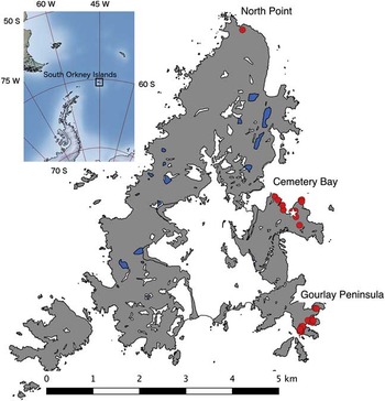
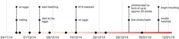
We collected in situ reflectance spectra at high spectral and spatial resolution from Signy Island, South Orkney Islands (Fig. 1), between November 2014 and January 2015. Signy is a small (c. 7×5 km), largely ice-covered island on which all three species of Pygoscelis penguins breed. Two of the authors (WGR, JAB) were based at the British Antarctic Survey (BAS) research station at Signy (60.709'S, 45.595'W) during this period. All the measurements described here were taken from samples of penguin guano, or penguin vomit, taken as being representative of the food being consumed within the colony. Data were collected from various sites around the island, but mainly from the extensive colonies of Adélie and chinstrap penguins located on the Gourlay Peninsula (60.729'S, 45.586'W). The period of data collection included most of the relevant breeding events for these two species, although the transition to predominantly pink guano was complete only for Adélie penguins (Fig. 2). Samples relating to gentoo penguins were mostly collected near North Point (60.672'S, 45.626'W) and Cemetery Bay (60.706'S, 45.603'W). Geographical coordinates are given in the WGS84 datum and with sufficient precision to allow colonies and sampling locations to be revisited.
Location of Signy Island and measurement sites (red dots). The white star indicates the position of the British Antarctic Survey research station. (Large-scale map data from Antarctic Digital Database: http://www.add.scar.org.)

Timeline showing data collection (diamonds) and key events for Adélie (circles) and chinstrap (squares) penguins. The bar at the bottom represents schematically the changing colour of guano.

Our sampling strategy was determined by our aim of collecting single-sample spectra covering the full range of spectral diversity of penguin guano as it evolved over time. It was not our intention to follow the spectral evolution of specific colonies over time, and it would not have been feasible to collect representative samples from the same colony at regular intervals. Our ability to access specific colonies was restricted by weather conditions, and our ability to move freely within colonies was restricted by the requirement not to disturb the penguins unnecessarily. Instead, we attempted as best we could to obtain spectra from samples that we judged, by eye, to be representative of any colony we visited at the time we visited it. We collected data from 68 guano samples, representing different Pygoscelis species, guano colours, stages of the breeding cycle and environmental conditions. Almost half of the samples were obtained from a single Adélie colony.
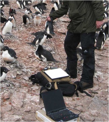
We used a FieldSpec Pro field-portable spectroradiometer (ASD, Boulder, CO, USA) to collect spectral data. This instrument detects radiation in the range 350–2500 nm, using three separate detection subsystems responding to the VNIR (350–970 nm), short-wave infrared 1 (SWIR1; 970–1750 nm) and short-wave infrared 2 (SWIR2; 1750–2500 nm) ranges. The spectral resolution of the instrument is c. 3 nm, 10 nm and 10 nm, respectively, in these three ranges. The ‘bare fibre’ fore-optic of the FieldSpec Pro was used, giving a field of view of c. 25° radius (typically 0.4 m at 0.8 m observing distance), which was normally sufficient to ensure that a homogeneous target material was being measured. For small samples the observing distance was reduced to c. 0.1 m, giving a field of view of radius c. 0.05 m. Reflectance values were subsequently calculated using measurements of a calibrated ‘Spectralon’ white panel reference which replaced the target material in the same geometrical configuration (Fig. 3). A set of measurements for a single sample consisted of at least three replicates (sample and white panel reference), together with a digital photograph of the sample. Since it was impossible to remove most guano samples for analysis in the laboratory, we relied on daylight to provide the illumination needed to take measurements in situ. It was important to ensure that illumination conditions remained constant during a set of measurements (i.e. for typically c. 5 min), and since conditions of continuous direct sunlight are not common on Signy Island this was usually not easy to achieve. We made frequent observations of sky conditions and monitored the intensity of incident light using a lux-meter.
Data collection. The sensor head is supported on a pole and alternately views the target and the Spectralon calibrator. The optical signal is carried by an optical fibre to the spectrometer (underneath the Spectralon panel), which is controlled by the laptop computer.

In addition to samples of penguin guano, measurements were also taken from samples of Adélie penguin vomit, i.e. the largely undigested stomach contents being carried by parents to feed chicks. Ten samples had been collected as part of a long-term monitoring project following CCAMLR ecosystem monitoring programme standard procedures (CCAMLR 1992) and made available to us for our spectral measurements after analysis of constituents had been carried out. Two very distinct types of vomit were observed: i) grey, predominantly fish-based and ii) pink, predominantly krill-based. We made our spectral measurements on these samples within at most three days of their collection, the samples having been frozen (and then thawed immediately prior to measurement) in the meantime.
We calculated the reflectance spectra for 62 of our 68 guano samples (the other six were not usable because of low light levels) and ten vomit samples using programs written in the GNU Octave language (Eaton et al. Reference Eaton, Bateman, Hauberg and Wehbring2015). In all cases it was impossible to retrieve meaningful spectra in the range 1830–1900 nm, and in most cases (where the incident light level was below c. 75 klx) the range 1350–1400 nm was also impossible to retrieve, owing to the effect of atmospheric water vapour absorbing all of the daylight illumination in these parts of the spectrum (Rees Reference Rees2013).
In order to try to identify a number of ‘generic’ spectra from our set of 62 spectra, they were generalized. First, the spectra were edited to include only the wavelength ranges 350–1350 and 1400–1800 nm; other wavelengths, including the SWIR2 band, were deemed to be too strongly affected by atmospheric water vapour absorption for the spectra to be reliable. Second, the data volume was reduced by averaging the spectra into 10 nm bins (i.e. 350–359, 370–369, … 1340–1349, 1400–1409, … 1790–1799 nm) so that each sample was represented by 140 variables. Then a statistical clustering method (agglomerative hierarchical clustering, using five different agglomeration methods and the Euclidean distance metric, implemented in the statistical package SPSS) was used to combine similar spectra into groups, allowing the method to guide the choice of the final number of groups. The dendrogram, showing dissimilarities between spectra, was then inspected to help choose the final number of groups into which the spectra should be combined. Possible associations between the groups and, firstly, penguin species and, secondly, guano colour and condition were investigated by calculating Cramér’s V statistic (Cramér Reference Cramér1999).
Results
Most spectra (n=31) were collected from a single large Adélie colony centred at 60.7312'S, 45.5884'W. Further Adélie spectra (n=9) were collected from a second colony centred at 60.7267'S, 45.58334'W. Chinstrap spectra were collected from colonies centred at 60.7295'S, 45.5841'W (n=2), 60.7304'S, 45.5880'W (n=4) and 60.7286'S, 45.5838'W (n=6). The remaining spectra were collected as indicated in Fig. 1. The visual appearance of most samples was white or pink, although some other colours were noted and measured including green and, especially in the case of gentoo penguins, yellow.
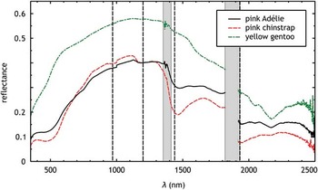
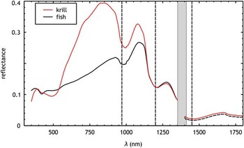
Only those few guano spectra collected when the ambient illumination exceeded c. 75 klx gave adequate representation of the entire spectral range, including the SWIR2 region, accessible by the FieldSpec Pro instrument. These spectra reveal an absence of any narrow spectral features, but do show some differences in the SWIR2 region (Fig. 4). There are broad absorption features, though not present in all the spectra, at c. 550, 1450 and 2150 nm. We were unable to calculate meaningful spectra for the vomit samples in the SWIR2 range, but the spectra in the range 350–1800 nm again revealed only broad spectral features (Fig. 5). The spectra of krill- and fish-based vomit are essentially identical in the range 1100–1800 nm and have common absorption features above c. 800 nm. Broad absorption features due to liquid water were very apparent at c. 950 and 1450 nm. In the VNIR region the spectra are substantially different, the krill-based vomit being generally more reflective, except around 500 nm. The sharp increase in reflectance between 500 and 700 nm is responsible for the visually strong red coloration. The high reflectance of the krill-based vomit sample between c. 700 and 1200 nm is very likely to be due to multiple scattering from undigested particles of chitin.
Full-range spectra: average spectra for pink Adélie and chinstrap, and yellow gentoo guano. Dashed lines show absorption peaks of liquid water. Grey bars show regions of the spectrum in which the atmosphere is particularly opaque as a result of water vapour absorption; the range from 1830–1900 nm was never measurable for this reason.

Vomit spectra measured for the range 350–1800 nm, excluding 1350–1400 nm. Dashed lines show absorption peaks of liquid water. The grey bar shows the region of the spectrum in which the atmosphere is particularly opaque as a result of water vapour absorption.

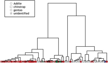
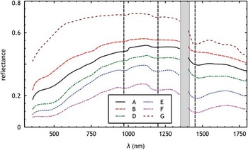
Generalization of the 62 guano spectra produced a reasonably clear indication that they could be combined into at most seven groups (Fig. 6), which are designated A to G. The average spectra were calculated for six of the seven groups (group C only had a single member and was not included in subsequent analyses). These average spectra again exhibited only broad spectral features, but were clearly differentiable on the basis of both average reflectance and depth of some spectral features (Fig. 7). Statistical analysis using Cramér’s V test showed that group membership is only weakly associated with penguin species, but it is more strongly associated with the colour and environmental state (whether wet or dry) of the guano.
Dendrogram from between-group hierarchical clustering. (Four other clustering methods were used giving slightly different histograms.) The shape of the symbol denotes the species, while the colour represents the visual appearance of the guano: white (or light yellow), pink, red, red/wet (shown as dark red), green or mixed (shown as blue).

Six average group spectra defined by clustering 62 spectra of penguin guano. The range 1350–1400 nm is excluded. Dashed lines show absorption peaks of liquid water. The grey bar shows the region of the spectrum in which the atmosphere is particularly opaque as a result of water vapour absorption.

Discussion
This study provides the first in situ well-defined reference spectra for guano of Adélie, chinstrap and gentoo penguins. The three general colours of guano deposits (pink, white and green) that are expected depending on food source were easily observed (Myrcha & Tatur Reference Myrcha and Tatur1991). These spectra show a well-represented change from white(ish) to pink during the breeding season, particularly for Adélie but also for chinstrap penguins. Pink guano is expected to arise from krill diets, white from fish diets and green from either undigested algae or bile when penguins are moulting and so not feeding (Heine & Speir Reference Heine and Speir1989). The presence of yellow guano in gentoo colonies, which was also accompanied by white and pink deposits, was surprising and may merit future investigation.
We interpret the generic spectra, represented by the groups A to G, as follows: Groups A and B are identified as white or light coloured dry samples of guano and are probably not truly distinct from one another. Their spectral shapes are very similar (Fig. 7) and the differences are probably due to a difference in wetness, with the wetter samples (group A) having lower reflectance. D is a group of dry but rather pinker guano samples, with a pronounced dip c. 550 nm superimposed on the generally rising trend in reflectance between 400–1000 nm. E is similar to D but with a rather stronger water absorption feature c. 1450 nm, and F is more extreme again; these groups correspond to pink-red samples with increasing degrees of wetness. Finally, the very distinct group G corresponds to optically thicker white or light coloured samples.
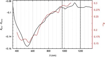
These six averaged spectra emphasize the importance of broad absorption features centred around 550 nm and 1450 nm in controlling differences between guano spectra (Fig. 4 also suggests a weak feature c. 1150 nm and that there is a feature in the SWIR2 region at c. 2200 nm). Narrow spectral features are not present and this suggests that high spectral resolution measurements may not be needed to identify penguin guano. The absorption feature at c. 550 nm is proposed to be due to the pigment astaxanthin, known to be responsible for the pink coloration of krill and other species (Fox Reference Fox1955, Auerswald et al. Reference Auerswald, Freier, Lopata and Meyer2008, Dissing et al. Reference Dissing, Nielsen, Ersbøll and Frosch2011). To verify this, Fig. 8 shows the difference between pink (group D) and white (average of groups A and B) guano reflectance plotted over the range 350–1350 nm, together with the experimentally determined reflectance spectrum of astaxanthin (Dissing et al. Reference Dissing, Nielsen, Ersbøll and Frosch2011). The correspondence between the two reflectance scales was established empirically. Although the two spectra differ in detail, there is good general correspondence in shape and location, lending support to the idea that the main principle responsible for the pink appearance of guano samples in this part of the spectrum is the presence of this pigment. This result, which is unsurprising, is also supported by comparison of Figs 4 and 5.
Published reflectance of astaxanthin (red, scale on right) compared with difference between pink and white guano determined in this work (black, scale on left). Dashed lines show absorption peaks of liquid water.

The other broad spectral features noted in Fig. 5 correspond well with the absorption maxima of liquid water at c. 970, 1200 and 1450 nm (Fig. 3 also shows evidence of a water absorption feature at c. 1930 nm). Of these, the most prominent is at 1450 nm. On this basis we propose two simple indices for distinguishing between different types and conditions of guano: a wetness index and a redness index. In terms of the Landsat-8 OLI bands, the wetness index is defined as:
 $${{{r_{5} {\minus}r_{6} } \over {r_{5} {\plus}r_{6} }}},$$
while the redness index is defined as:
 $${{{r_{4} {\minus}r_{3} } \over {r_{4} {\plus}r_{3} }}}.$$
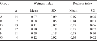
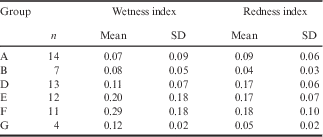
The wavelength ranges of these bands are 3 (530–590 nm), 4 (640–670 nm), 5 (850–880 nm) and 6 (1570–1650 nm). The values of these two indices for the six average spectra shown in Fig. 7 are shown in Table I. As a result of the limitations on systematic sampling noted earlier, it is not possible to make a useful statement about trends in these indices over time. However, we can cautiously identify some tendencies in the Adélie data, for which there is the largest number of measurements.
Wetness and redness indices calculated for the six groups (A, B, D–G) shown in Fig. 7.
SD=standard deviation.
None of the samples that were collected in late November showed a redness index>0.1, while almost all samples that were collected after this date showed higher values in the redness index. We suggest that this pattern, which was also observed (though at a later date) for chinstrap penguin guano, could be used to quantify the phenomenon of pinking-up of guano. Variation in penguin breeding phenology is known to occur (Black Reference Black2016), including between separate subcolonies of the same species at the same location (Trathan, personal observation Monroe Island 2015/2016), and this quantitative approach, applied to suitable multispectral remote sensing imagery, could allow variability in breeding phenology to be investigated. The ‘wetness’ index of nearly all samples is below c. 0.25, except for the measurements obtained on 21 December when much higher values were noted. These samples were all obtained from sites on the Gourlay Peninsula, a couple of days after snowfall which had partially melted. The effect of liquid water on the distribution and appearance of the guano was very marked on this occasion; it resembled a waterlogged red clay soil or a very thick beetroot soup. Despite the very high values of the wetness index from these measurements, the redness index was within the normal range, confirming the ability of the two indices to separate the effects of the pinking-up and environmental processes in controlling the guano reflectance. It is important to note here that these indices have been derived from measurements taken from single homogeneous samples of guano. Calculating the same indices for the pixels of a satellite image will invoke the ‘mixed pixel’ problem, which is likely to increase the extent to which the indices vary over time as the coverage of guano, both as an areal percentage and as thickness, increases.
Although our results do not suggest that it is possible to discriminate between Pygoscelis penguin species on the basis of the spectral properties of their guano alone, the spectrally distinctive redness signal suggests that it may be possible to deduce the phenological stage from suitable imagery and hence to infer the species. Our observations of the visual differences between chinstrap and Adélie colonies, at a time when most Adélie chicks had hatched but most chinstrap chicks had yet to do so, certainly suggest that this should be possible, and use of the wetness index should reduce possible ambiguities in the interpretation of guano-dominated spectra. It is possible that the difference between Adélie and chinstrap colonies might decrease in subsequent weeks as the chinstrap chicks grow, so further measurements would be beneficial.
The redness and wetness indices proposed here represent a relatively simple approach to extracting physically or physiologically meaningful data from spectra. They can probably be extended. There is perhaps a suggestion in the group spectra presented in Fig. 7 that the astaxanthin absorption feature broadens as the pigment concentration increases. If so, this could potentially be exploited by examining derivatives of the spectral reflectance functions (which should therefore not be smoothed to 10 nm spectral resolution). Both indices could perhaps be standardized between different guano types, although that would require more data than were collected for this work.
We can ask what more would be needed to develop the results presented here into a robust algorithm for identifying Antarctic penguin colonies and estimating the number of birds within them. That remains a difficult goal to reach, though it is nearer. At least for krill-feeding species where the astaxanthin signal in the pink guano can be recognized, the major difficulties will be obtaining imagery at sufficiently high spatial resolution and at the right time of year, and understanding better the spatial characteristics of penguin colonies (including variations in packing densities). Future work should focus on determining how much guano spectra influence colony spectra (what extent of spatial mixing there is), as well as what level of spatial resolution is necessary for accurate colony examination especially given the high costs of higher resolution imagery and the need for low cost penguin counts.
Conclusions
The fundamental aim of this research was to define ‘generic’ spectra for the guano of Pygoscelis penguins at very high spectral and spatial resolution, and this has been accomplished. These data will provide a baseline for the development of improved methods for detecting and analysing Antarctic penguin colonies. As has been noted and exploited in previous work, breeding colonies ‘pink up’ as the diet shifts to one rich in krill. The reason for this pink coloration is unambiguously attributable to the pigment astaxanthin responsible for the pinkness of the krill itself. Apart from the presence of this pigment, the other main factor controlling the optical properties of the majority of penguin guano at this stage in the breeding cycle is environmental processing through waterlogging. We propose two simple mathematical indices, based on reflectance values in the red and near infrared parts of the spectrum, that can be calculated from satellite imagery and that allow the influences of astaxanthin and environmental conditions to be separated. The ability to extract a separate ‘redness’ signal has the potential to allow the pinking-up process to be tracked over time in a series of images, which would help to distinguish between species, although in practice this ability will be compromised by the difficulty of obtaining a time series of images from a location such as Signy with very frequent cloud cover. The data collected during the fieldwork for this research did not reveal any systematic differences between the spectra of guano from different penguin species, which is probably unsurprising in view of the very marked effect of diet on the spectra. Taken together, these results should significantly enhance our ability to recognize penguins from guano stains in satellite images and understand the potential differences in coloration of guano.
Acknowledgements
The fieldwork necessary for this work was supported by BAS through a Collaborative Gearing Scheme award CGS-97 to W.G. Rees and P.N. Trathan, and the ASD FieldSpec Pro was made available through an award (ref. 696.0614) from the UK NERC Field Spectroscopy Facility. We acknowledge with gratitude the support and companionship of the entire staff of the BAS research station at Signy, and especially of M. Jobson, the Base Commander. We gratefully acknowledge also the input of S. Adlard, who was generous in sharing her understanding of Signy’s penguin population and her samples of penguin vomit. J.A. Brown is supported by a NERC PhD studentship NE/L501633/1. We gratefully acknowledge the constructive criticisms of a number of reviewers that have materially improved this paper.
Processed reflectance spectra and accompanying sample photographs will be available at the University of Cambridge research repository (https://doi.org/10.17863/CAM.8273) from 1 January 2018.
Author contribution
WGR and JAB performed the data collection and analysis. All authors contributed equally to writing the paper.