1 Introduction
Consider a viscous suspension of spherical conducting particles subject to a shear flow placed in a uniform magnetic field. The fluid strain rate induces particle rotation; in the absence of any external torque, the particle angular velocity is equal to one half of the fluid vorticity. However, eddy currents are induced within a conductor rotating in a magnetic field due to Faraday’s law of induction. The eddy currents impart a magnetic dipole moment to the particle due to Ampere’s law. The interaction of the induced magnetic moment with the applied magnetic field results in an eddy current torque on the particle (Halverson & Cohen Reference Halverson and Cohen1964; Landau, Lifshitz & Pitaevskii Reference Landau, Lifshitz and Pitaevskii2014). Due to the eddy current torque, the particle rotation rate is different from the fluid rotation rate, and there is a net torque exerted by the particle on the fluid. There is an antisymmetric contribution to particle stress in the plane perpendicular to the torque when the particles exert a net torque on the fluid (Batchelor Reference Batchelor1970). If the magnetic field is perpendicular to the fluid vorticity, the antisymmetric particle stress is in the flow–gradient plane perpendicular to the fluid vorticity. If the magnetic field is not perpendicular to the fluid vorticity, the torque has a ‘precession’ component perpendicular to the vorticity–magnetic field plane. In this case, there are antisymmetric contributions to the stress perpendicular to all three axes. The antisymmetric particle stress due to the eddy current torque in a viscous (zero inertia) suspension of conducting particles subject to a magnetic field in the dilute (non-interacting) limit is the subject of the present study.
The rheology and yielding behaviour of magnetorheological fluids have been the subject of many studies (de Vicente, Klingenberg & Hidalgo-Alvarez Reference de Vicente, Klingenberg and Hidalgo-Alvarez2011). Magnetorheological fluids consist of magnetic particles with size in the range of microns to nanometres suspended in a viscous carrier fluid. When a magnetic field is applied, the viscosity of the fluid could increase by many orders of magnitude, resulting in a transition from a fluid to a solid-like state within a time period of a few milliseconds. In the presence of a magnetic field, a magnetorheological fluid exhibits a very high yield stress. Due to the fast switching between fluid-like and solid-like states and the high yield stress in the solid-like state, magnetorheological fluids are used in applications such as dampers, shock absorbers, clutches and brakes (Klingenberg Reference Klingenberg2001). The parameter governing the switching between the fluid-like and solid-like states is the Mason number, which is the ratio of the torque on the particle due to the shear flow and that due to the magnetic moment of the particle. A second parameter is denoted
 $\unicode[STIX]{x1D706}$
, the ratio of the energy of the magnetic interaction between the pair of particles and the thermal energy which results in Brownian diffusion of the particle orientation. For high
 $\unicode[STIX]{x1D706}$
(where the magnetic interaction energy is much larger than the thermal energy) and below a critical Mason number, there is an increase of many orders of magnitude in the viscosity. This is because the particles are magnetised in the presence of the field, they align parallel to the field lines and jam the suspension (Anupama, Kumaran & Sahoo Reference Anupama, Kumaran and Sahoo2018). The reason for the high viscosity and the high yield stress has been the subject of many studies, starting with studies on the constitutive relations for a dilute suspension of magnetic particles (Jansons Reference Jansons1983), dynamic rheology under oscillatory shear and the effect of shape on the rheology (de Vicente et al.
Reference de Vicente, Segovia-Gutierrez, Andablo-Reyes, Vereda and Hidalgo-Alvarez2009) and the rheology of suspensions of magnetic fibres (Kuzhir, Lopez-Lopez & Bossis Reference Kuzhir, Lopez-Lopez and Bossis2009; Lopez-Lopez, Kuzhir & Bossis Reference Lopez-Lopez, Kuzhir and Bossis2009). The critical Mason number has been related to the Bingham number, which is the ratio of the yield stress and the viscous stress (Sherman, Becnel & Wereley Reference Sherman, Becnel and Wereley2015). The instabilities in thin films of magnetic particles due to an applied electric field (Seric, Afkhami & Kondic Reference Seric, Afkhami and Kondic2014) and the turbulence in fluid suspensions with magnetic particles (Schumacher, Riley & Finlayson Reference Schumacher, Riley and Finlayson2008) have also been studied. The yield stress is one of the salient properties of a magnetorheological fluid, and models for the yield stress include macroscopic models based on magnetic energy minimisation of particle aggregates (Bossis et al.
Reference Bossis, Lemaire, Volkova and Clercx1997) and microscopic particle-based models (Klingenberg & Zukoski Reference Klingenberg and Zukoski1990; Vagberg & Tighe Reference Vagberg and Tighe2017).
The rheology of a suspension of conducting particles made of materials such as aluminium or copper has received relatively less attention. Though all materials, paramagnetic or diamagnetic, do develop a small magnetic moment under the influence of a magnetic field, this effect is extremely weak and indiscernible in most cases. However, when the particles are rotated by shear, there is an eddy current induced in a particle, which imparts a magnetic moment. The interaction of the induced moment and the external field results in a torque on the particle, which acts in the direction opposite to the particle angular velocity. The torque on spherical particles and shells rotating with a known angular velocity has been solved using the Maxwell equations assuming a quasi-static electromagnetic field. For paramagnetic and diamagnetic materials, the relative magnetic permeability is very close to
 $1$
, and magnetic permeability is assumed to be the vacuum permeability
 $\unicode[STIX]{x1D707}_{0}$
. An important approximation is that in Ampere’s law
 $\unicode[STIX]{x1D735}\times \boldsymbol{H}=\boldsymbol{J}+\unicode[STIX]{x1D716}(\unicode[STIX]{x2202}\boldsymbol{E}/\unicode[STIX]{x2202}t)$
for the magnetic field
 $\boldsymbol{H}$
, the term proportional to the time derivative of the electric field
 $\unicode[STIX]{x1D716}(\unicode[STIX]{x2202}\boldsymbol{E}/\unicode[STIX]{x2202}t)$
is neglected in comparison to the current density
 $\boldsymbol{J}$
. Here,
 $\unicode[STIX]{x1D716}$
is the dielectric constant of the material. Since the electric field and current density are related by Ohm’s law,
 $\unicode[STIX]{x1D71A}\boldsymbol{J}=\boldsymbol{E}$
, where
 $\unicode[STIX]{x1D71A}$
is the resistivity of the material, the quasi-static approximation is valid for
 $(\unicode[STIX]{x1D716}\unicode[STIX]{x1D6FA}/\unicode[STIX]{x1D71A})\ll 1$
, where
 $\unicode[STIX]{x1D6FA}$
is the angular velocity. The ratio
 $(\unicode[STIX]{x1D716}/\unicode[STIX]{x1D71A})$
, the mean free time for electrons in a conductor, is of the order of
 $10^{-14}$
s. Therefore, the product of the angular velocity and the mean free time is small in practical situations, and Ampere’s law is quasi-steady. There is, however, time dependence in Faraday’s law of induction. Using the quasi-static approximation for Ampere’s law, the torque on a rotating sphere and a rotating spherical shell in a magnetic field have been calculated (Halverson & Cohen Reference Halverson and Cohen1964; Landau et al.
Reference Landau, Lifshitz and Pitaevskii2014).
The torque on a rotating shell in a magnetic field is used for modelling the decrease in the angular velocity of satellites which orbit the Earth (Habib et al. Reference Habib, Holz, Kheyfets, Matzner, Miller and Tolman1994). In his pioneering work on the force and torque due to eddy currents, Moffat (Reference Moffat1990) considered prototypical time-varying magnetic fields such as rotating and traveling fields. The trajectory of a particle in a specified time-varying magnetic field was calculated, and the effect of particle interactions on the trajectories of multiple particles was also determined. Experiments (Bolcato et al. Reference Bolcato, Etay, Fautrelle and Moffatt1993) have also been conducted on the motion of metallic particles in a time-varying magnetic field. Here, a simpler configuration is considered where the magnetic field is steady, but the suspension is subjected to a shear flow with a rotational component which rotates the particles. In the viscous limit, the particle and fluid rotation rates are equal in the absence of an external torque. However, when there is a magnetic field, the eddy current due to particle rotation results in a torque which tends to decrease the rotation rate, resulting in a difference between the particle and the fluid rotation rates. The torque exerted by the particles on the fluid results in an antisymmetric contribution to the particle stress tensor (Batchelor Reference Batchelor1970).
The antisymmetric part of the stress tensor due to the eddy current torque is different from that in ‘couple stress fluids’ or ‘Cosserat continua’ (Truesdell & Toupin Reference Truesdell, Toupin and Flugge1960; Mindlin & Tiersten Reference Mindlin and Tiersten1962; Stokes Reference Stokes1966). In the latter, there is an antisymmetric contribution to the stress tensor due to the gradient in the vorticity in the fluid, and a contribution due to the ‘body torque’. The present system is qualitatively different from couple stress fluids, because the body torque due to the particles is related to the difference in the particle angular velocity and the fluid rotation rate; the particle angular velocity is in turn determined by the torque balance condition that the sum of the hydrodynamic and magnetic torques is zero in the absence of inertia. Therefore, the couple stress due to the body torque is a function of the local fluid vorticity, and not the gradient of the fluid vorticity as assumed in couple stress fluids. Moreover, the eddy current torque is a nonlinear function of the particle angular velocity, so the couple stress coefficients (ratios of the antisymmetric components of the stress tensor and the vorticity) are functions of the angular velocity.
The torque on a conducting particle in a magnetic field due to induced eddy currents is summarised in § 2, and a detailed calculation is provided in appendix A. Two types of particles are considered, a uniform sphere of radius
 $R$
and a thin shell of radius
 $R$
and thickness
 $\unicode[STIX]{x1D6FF}R$
with
 $\unicode[STIX]{x1D6FF}\ll 1$
. The torque on a uniform spherical particle is a classical problem (Landau et al.
Reference Landau, Lifshitz and Pitaevskii2014). The torque on a spherical shell has been calculated using phaser notation (Halverson & Cohen Reference Halverson and Cohen1964), but this calculation is unnecessarily complicated and tedious, and so a simpler derivation has been provided in appendix A. The relation between the torque and the angular velocity is inherently nonlinear, as shown in § 2. Moreover, the torque is not confined to the plane containing the angular velocity and magnetic field, but there could be a component of the torque (called the precession torque) which is perpendicular to the plane containing the angular velocity and the magnetic field. Whereas the torque on a particle is determined as a function of a known angular velocity in appendix A, it is necessary here to determine the angular velocity from a balance between the hydrodynamic and eddy current torques. The relationship between the eddy current torque and the angular velocity is nonlinear, and it is not possible to obtain an explicit solution for the magnitude and direction of the particle angular velocity for known vorticity and magnetic field. An implicit solution procedure is formulated in § 2.
The particle stress due to the torque exerted by the particles, first discussed by Batchelor (Reference Batchelor1970), is briefly summarised in § 3. The calculation is restricted to the dilute limit where the particles are non-interacting, that is, the velocity disturbance around one particle does not affect the dynamics of another. The primary objective here is to define the couple stress coefficients in the relation between the antisymmetric part of the particle stress tensor and the fluid vorticity. The antisymmetric part of the stress tensor is resolved in three planes, each of which is perpendicular to one of three orthogonal directions. The first couple stress is in the plane perpendicular to the direction of the vorticity vector, the second couple stress is perpendicular to the unit normal to the vorticity in the vorticity–magnetic field plane, the third couple stress is in the plane containing the vorticity and the magnetic field. The first and second couple stress coefficients are not independent, but are related due to the requirement that the torque is necessarily perpendicular to the magnetic field. This relation is derived in § 3.
The couple stress coefficients for an oblique magnetic field, where the vorticity and the magnetic field are not perpendicular, is calculated in § 4 based on the requirement that the sum of the hydrodynamic and magnetic torques is zero. The solutions depend on two parameters, the first of which is the ratio of the characteristic magnetic and hydrodynamic torque,
 $\unicode[STIX]{x1D6F4}=(\unicode[STIX]{x1D707}_{0}H_{0}^{2}/4\unicode[STIX]{x03C0}\unicode[STIX]{x1D702}|\unicode[STIX]{x1D74E}|)$
, where
 $\unicode[STIX]{x1D707}_{0}$
is the magnetic permeability,
 $H_{0}$
is the magnitude of this magnetic field,
 $\unicode[STIX]{x1D702}$
is the fluid viscosity and
 $\unicode[STIX]{x1D74E}$
is the fluid vorticity at the particle location. This parameter
 $\unicode[STIX]{x1D6F4}$
is similar to the inverse of the Mason number for magnetorheological fluids, but with one important difference, that it is based on the fluid vorticity at the particle centre, in contrast to the Mason number, which is based on the fluid strain rate. The parameter
 $\unicode[STIX]{x1D6F4}$
here is defined as the ratio of the magnetic and hydrodynamic torques, whereas the Mason number is the ratio of the viscous and magnetic stresses. It is appropriate to define the dimensionless parameter as the inverse of the Mason number for the present problem, because a magnetic moment is induced in the particles only when subjected to rotation; this is in contrast to particles in a magnetorheological fluid which are polarised by an applied magnetic field even in the static state. The limit of zero Mason number can be realised for a magnetorheological fluid by turning off the flow, but it is a singular limit for conducting particles because there is no eddy current in stationary particles. The subject of this study is the rheology modification due to the magnetic moment induced in the particles, and so it is appropriate to consider the control parameter
 $\unicode[STIX]{x1D6F4}$
as the ratio of the characteristic magnetic and the hydrodynamic torques.
The second dimensionless parameter is
 $\unicode[STIX]{x1D6FD}$
, the product of the fluid vorticity and the eddy current relaxation time, which has no analogue in magnetorheological fluids. For a uniform particle,
 $\unicode[STIX]{x1D6FD}=\unicode[STIX]{x1D6FD}_{p}=(|\unicode[STIX]{x1D74E}|\unicode[STIX]{x1D707}_{0}R^{2}/2\unicode[STIX]{x1D71A})$
, where
 $R$
is the particle radius and
 $\unicode[STIX]{x1D71A}$
is the electrical resistivity. For a thin shell,
 $\unicode[STIX]{x1D6FD}=\unicode[STIX]{x1D6FD}_{s}=(|\unicode[STIX]{x1D74E}|\unicode[STIX]{x1D707}_{0}R^{2}\unicode[STIX]{x1D6FF}/2\unicode[STIX]{x1D71A})$
, where
 $R$
is the particle diameter,
 $R\unicode[STIX]{x1D6FF}$
is the shell thickness and
 $\unicode[STIX]{x1D6FF}\ll 1$
. Asymptotic results are derived in § 4 for the particle angular velocity and the couple stress coefficients in the limits
 $\unicode[STIX]{x1D6F4}\ll 1$
and
 $\unicode[STIX]{x1D6F4}\gg 1$
, and numerical solutions are obtained for the intermediate
 $\unicode[STIX]{x1D6F4}$
, for a comprehensive understanding of the rheology modification in different parameter regimes.
The subject of § 5 is the special case where the fluid vorticity and magnetic field are orthogonal. In this case, the particle angular velocity vector is parallel to the vorticity, and only the first couple stress coefficient (perpendicular to the vorticity and in the velocity–velocity gradient plane) is non-zero. An interesting observation here is the possibility of multiple solutions for the particle angular velocity and the couple stress coefficient at sufficiently high values of
 $\unicode[STIX]{x1D6FD}$
. This is due to the nonlinear relationship between the torque and the angular velocity in the balance equation for the torque in the vorticity direction. The parameter regimes for multiple steady states are identified using asymptotic analysis in the limit
 $\unicode[STIX]{x1D6FD}\gg 1$
, and numerical solutions are obtained for finite but large
 $\unicode[STIX]{x1D6FD}$
. In § 6, multiple steady states are also found for a near-perpendicular magnetic field when the cosine of the angle between the vorticity and the magnetic field is less than
 $1/3$
. The reason for this, which is the nonlinear relationship between the precession torque (perpendicular to the plane containing the vorticity and magnetic field) and the angular velocity, is qualitatively different than that for a perpendicular magnetic field. Asymptotic analysis is also used to explain the physical reason, and to identify the parameter regimes for the existence of multiple steady states, in § 6.
The effect of inter-particle interactions and particle migration due to a gradient in the angular velocity and the fluid vorticity is briefly discussed in appendix D. A noteworthy result is that there are no difficulties due to divergences with system size such as those encountered in the velocity of settling spheres (Batchelor Reference Batchelor1972; Hinch Reference Hinch1977; Caflisch & Luke Reference Caflisch and Luke1985) or the variance of the sedimentation velocity (Koch & Shaqfeh Reference Koch and Shaqfeh1991; Guazzelli & Hinch Reference Guazzelli and Hinch2011) due to the slowly decreasing nature of the velocity disturbance caused by a particle in the absence of inertia. In appendix D, particle migration due to gradients in the particle angular velocity, volume fraction and vorticity are also calculated. Faxen’s law has been used to calculate the particle migration due to a gradient in the fluid strain rate by Hogg (Reference Hogg1994) for a zero Reynolds number flow in a parabolic velocity profile. In § D.4, this calculation is briefly extended to the case where there is a gradient in the fluid vorticity, and this results in a particle drift proportional to the curl of the vorticity. The inertial migration of particles (Saffman Reference Saffman1965; Ho & Leal Reference Ho and Leal1974) is not considered here.
The couple stress coefficients depend on the parameters
 $\unicode[STIX]{x1D6F4}$
and
 $\unicode[STIX]{x1D6FD}$
, as well as the unit vectors
 $\hat{\unicode[STIX]{x1D74E}}$
and
 $\hat{\boldsymbol{H}}$
in the directions of the angular velocity and the magnetic field respectively. In the analysis, the unit vectors
 $\hat{\unicode[STIX]{x1D74E}}$
and
 $\hat{\boldsymbol{H}}$
, and the dot and cross products
 $\hat{\unicode[STIX]{x1D74E}}\boldsymbol{\cdot }\hat{\boldsymbol{H}}$
and
 $\hat{\boldsymbol{H}}\boldsymbol{\times }\hat{\unicode[STIX]{x1D74E}}$
, are explicitly written, instead of expressing these in terms of the cosine or sine of the angle between the vorticity and the magnetic field. Though this appears a little unwieldy, this notation enables easy application of the results to cases where the vorticity and magnetic field are not aligned with any of the configuration-based axes. There could also be situations where the vorticity at the particle centre and the magnetic field are in different directions for different particles. In such cases, the results derived here could be used to compute the torque and angular velocity of individual particles in particle-based simulations. The notations are explained in detail at the beginning of the following § 2 before proceeding to the calculation of the torque on a particle.
2 Torque on a particle
The notations used in the analysis are first explained to enhance clarity. The particle angular velocity vector, fluid vorticity vector and magnetic field vector are denoted
 $\unicode[STIX]{x1D734}$
,
 $\unicode[STIX]{x1D74E}$
and
 $\boldsymbol{H}_{0}$
respectively. The unit vectors in the direction of the particle angular velocity, fluid vorticity and the applied magnetic field are designated
 $\hat{\unicode[STIX]{x1D734}}$
,
 $\hat{\unicode[STIX]{x1D74E}}$
and
 $\hat{\boldsymbol{H}}$
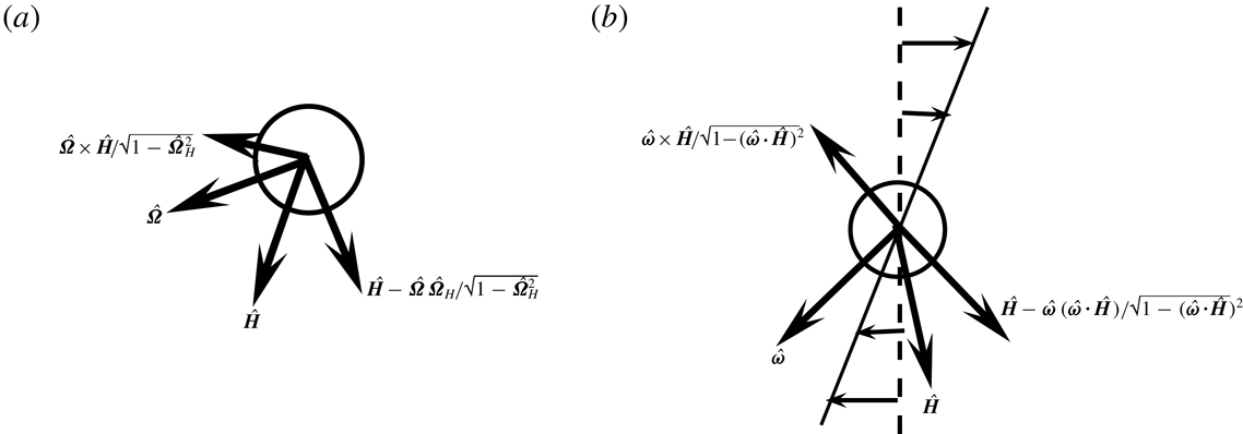
respectively, as shown in figure 1. The projection of the unit angular velocity vector
 $\hat{\unicode[STIX]{x1D734}}$
on to the direction of the magnetic field is defined as
 $\hat{\unicode[STIX]{x1D6FA}}_{\boldsymbol{H}}$
,
 $$\begin{eqnarray}\displaystyle \hat{\unicode[STIX]{x1D6FA}}_{\boldsymbol{H}}=\hat{\unicode[STIX]{x1D734}}\boldsymbol{\cdot }\hat{\boldsymbol{H}}, & & \displaystyle\end{eqnarray}$$
and the projection on to the direction of the fluid vorticity is defined as
 $\hat{\unicode[STIX]{x1D6FA}}_{\unicode[STIX]{x1D74E}}$
,
 $$\begin{eqnarray}\displaystyle \hat{\unicode[STIX]{x1D6FA}}_{\unicode[STIX]{x1D74E}}=\hat{\unicode[STIX]{x1D734}}\boldsymbol{\cdot }\hat{\unicode[STIX]{x1D74E}}. & & \displaystyle\end{eqnarray}$$
The scalar product of the unit vectors in the vorticity and the magnetic field directions is explicitly written as
 $\hat{\unicode[STIX]{x1D74E}}\boldsymbol{\cdot }\hat{\boldsymbol{H}}$
throughout the analysis for reasons explained at the end of the introduction. There are two distinct parts in the analysis, the first where the eddy current torque is calculated for a specified particle angular velocity, and the second where the angular velocity is determined by setting the sum of the hydrodynamic and eddy current torques equal to zero. In the first part, an orthonormal coordinate system shown in figure 1(a) is used where the first unit vector is along the angular velocity
 $\hat{\unicode[STIX]{x1D734}}$
, the second unit vector (
 $(\hat{\boldsymbol{H}}-\hat{\unicode[STIX]{x1D6FA}}_{\boldsymbol{H}}\hat{\unicode[STIX]{x1D734}})/\sqrt{1-\hat{\unicode[STIX]{x1D6FA}}_{\boldsymbol{H}}^{2}}$
) is perpendicular to
 $\hat{\unicode[STIX]{x1D734}}$
in the
 $\hat{\boldsymbol{H}}{-}\hat{\unicode[STIX]{x1D734}}$
plane and the third unit vector
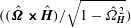 $((\hat{\unicode[STIX]{x1D734}}\boldsymbol{\times }\hat{\boldsymbol{H}})/\sqrt{1-\hat{\unicode[STIX]{x1D6FA}}_{\boldsymbol{H}}^{2}})$
is perpendicular to the
 $\hat{\boldsymbol{H}}{-}\hat{\unicode[STIX]{x1D734}}$
plane. In the second part where the angular velocity is calculated for specified vorticity and magnetic field, an orthonormal coordinate system shown in figure 1(b) is used where the first unit vector is in the vorticity direction
 $\hat{\unicode[STIX]{x1D74E}}$
, the second
 $((\hat{\boldsymbol{H}}-\hat{\unicode[STIX]{x1D74E}}(\hat{\unicode[STIX]{x1D74E}}\boldsymbol{\cdot }\hat{\boldsymbol{H}}))/\sqrt{1-(\hat{\unicode[STIX]{x1D74E}}\boldsymbol{\cdot }\hat{\boldsymbol{H}})^{2}})$
is perpendicular to
 $\hat{\unicode[STIX]{x1D74E}}$
in the
 $\hat{\boldsymbol{H}}{-}\hat{\unicode[STIX]{x1D74E}}$
plane and the third unit vector
 $((\hat{\unicode[STIX]{x1D74E}}\boldsymbol{\times }\hat{\boldsymbol{H}})/\sqrt{1-(\hat{\unicode[STIX]{x1D74E}}\boldsymbol{\cdot }\hat{\boldsymbol{H}})^{2}})$
is perpendicular to the
 $\hat{\boldsymbol{H}}{-}\hat{\unicode[STIX]{x1D74E}}$
plane. The components of the unit angular velocity vector,
 $\hat{\unicode[STIX]{x1D734}}$
, along the direction perpendicular to
 $\hat{\unicode[STIX]{x1D74E}}$
in the
 $\hat{\unicode[STIX]{x1D74E}}{-}\hat{\boldsymbol{H}}$
plane is defined as
 $\hat{\unicode[STIX]{x1D6FA}}_{\Vert }$
,
 $$\begin{eqnarray}\displaystyle \hat{\unicode[STIX]{x1D6FA}}_{\Vert }=\frac{(\hat{\unicode[STIX]{x1D6FA}}_{\boldsymbol{H}}-\hat{\unicode[STIX]{x1D6FA}}_{\unicode[STIX]{x1D74E}}\hat{\unicode[STIX]{x1D74E}}\boldsymbol{\cdot }\hat{\boldsymbol{H}})}{\sqrt{1-(\hat{\unicode[STIX]{x1D74E}}\boldsymbol{\cdot }\hat{\boldsymbol{H}})^{2}}}, & & \displaystyle\end{eqnarray}$$
and the component of the unit angular velocity vector perpendicular to the
 $\hat{\unicode[STIX]{x1D74E}}{-}\hat{\boldsymbol{H}}$
plane is defined as
 $\hat{\unicode[STIX]{x1D6FA}}_{\bot }$
,
 $$\begin{eqnarray}\displaystyle \hat{\unicode[STIX]{x1D6FA}}_{\bot }=\frac{\hat{\unicode[STIX]{x1D734}}\boldsymbol{\cdot }(\hat{\unicode[STIX]{x1D74E}}\boldsymbol{\times }\hat{\boldsymbol{H}})}{\sqrt{1-(\hat{\unicode[STIX]{x1D74E}}\boldsymbol{\cdot }\hat{\boldsymbol{H}})^{2}}}. & & \displaystyle\end{eqnarray}$$
Coordinate system for the torque on a particle with angular velocity
 $\unicode[STIX]{x1D734}$
rotating in a magnetic field
 $\boldsymbol{H}_{0}$
(a), and for the angular velocity of a particle in a flow field with vorticity
 $\unicode[STIX]{x1D74E}$
and magnetic field strength
 $\boldsymbol{H}_{0}$
(b). The hatted symbols are unit vectors in the respective directions. In (b) the direction of the vorticity vector is perpendicular to the flow plane for a simple shear flow.

The hydrodynamic torque exerted by the fluid on the particle is
 $8\unicode[STIX]{x03C0}\unicode[STIX]{x1D702}R^{3}((\unicode[STIX]{x1D74E}/2)-\unicode[STIX]{x1D734})$
, where
 $\unicode[STIX]{x1D702}$
is the fluid viscosity,
 $R$
is the particle radius and
 $\unicode[STIX]{x1D74E}$
is the far-field vorticity vector at the particle centre calculated in the absence of the particle. The expressions for the eddy current torque are derived in appendix A for a uniform particle of radius
 $R$
and constant electrical resistivity, as well as for a thin conducting shell whose thickness
 $\unicode[STIX]{x1D6FF}R$
is small compared to the radius. In the torque balance equations, the sum of the hydrodynamic and eddy current torque is set equal to zero in the three coordinate directions. Along the direction of the angular velocity, the hydrodynamic torque is
 $8\unicode[STIX]{x03C0}\unicode[STIX]{x1D702}R^{3}((\unicode[STIX]{x1D74E}/2)-\unicode[STIX]{x1D734})\boldsymbol{\cdot }\hat{\unicode[STIX]{x1D734}}$
, and the eddy current torque is given by
 $T_{z}$
in (A 27), where
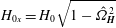 $H_{0x}=H_{0}\sqrt{1-\hat{\unicode[STIX]{x1D6FA}}_{\boldsymbol{H}}^{2}}$
is the component of the magnetic field perpendicular to
 $\unicode[STIX]{x1D734}$
in the
 $\boldsymbol{H}_{0}{-}\unicode[STIX]{x1D734}$
plane, and
 $H_{0}$
is the magnitude of the magnetic field. It is convenient to scale the torque balance equation by the magnitude of the hydrodynamic torque in the absence of particle rotation,
 $4\unicode[STIX]{x03C0}\unicode[STIX]{x1D702}R^{3}|\unicode[STIX]{x1D74E}|$
, to obtain the following angular momentum balance equation along the direction of
 $\hat{\unicode[STIX]{x1D734}}$
,
 $$\begin{eqnarray}\displaystyle \hat{\unicode[STIX]{x1D6FA}}_{\unicode[STIX]{x1D74E}}-\unicode[STIX]{x1D6FA}^{\ast }-\unicode[STIX]{x1D6F4}(1-\hat{\unicode[STIX]{x1D6FA}}_{\boldsymbol{H}}^{2})M_{I}(\unicode[STIX]{x1D6FD}\unicode[STIX]{x1D6FA}^{\ast }) & = & \displaystyle 0,\end{eqnarray}$$
where
 $\unicode[STIX]{x1D6FA}^{\ast }=(|\unicode[STIX]{x1D734}|)/(|\unicode[STIX]{x1D74E}|/2)$
is the particle angular velocity scaled by one half of the vorticity,
 $\unicode[STIX]{x1D6F4}=(\unicode[STIX]{x1D707}_{0}H_{0}^{2}/4\unicode[STIX]{x03C0}\unicode[STIX]{x1D702}|\unicode[STIX]{x1D74E}|)$
is the dimensionless ratio of the characteristic eddy current torque and the hydrodynamic torque,
 $\unicode[STIX]{x1D707}_{0}$
is the magnetic permeability of free space and the dimensionless parameter
 $\unicode[STIX]{x1D6FD}$
is the product of the current relaxation time and the vorticity which is discussed a little later. In the direction
 $(\hat{\boldsymbol{H}}-\hat{\unicode[STIX]{x1D6FA}}_{\boldsymbol{H}}\hat{\unicode[STIX]{x1D734}})/\sqrt{1-\hat{\unicode[STIX]{x1D6FA}}_{\boldsymbol{H}}^{2}}$
, the hydrodynamic torque is
 $4\unicode[STIX]{x03C0}\unicode[STIX]{x1D702}R^{3}\unicode[STIX]{x1D74E}\boldsymbol{\cdot }(\hat{\boldsymbol{H}}-\hat{\unicode[STIX]{x1D6FA}}_{\boldsymbol{H}}\hat{\unicode[STIX]{x1D734}})/\sqrt{1-\hat{\unicode[STIX]{x1D6FA}}_{\boldsymbol{H}}^{2}}$
, and the eddy current torque is given by
 $T_{x}$
in (A 27), where
 $H_{0z}=H_{0}\hat{\unicode[STIX]{x1D6FA}}_{\boldsymbol{H}}$
is the component of the magnetic field in the direction of the angular velocity, and
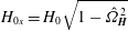 $H_{0x}=H_{0}\sqrt{1-\hat{\unicode[STIX]{x1D6FA}}_{\boldsymbol{H}}^{2}}$
. When the torque balance equation is divided by
 $4\unicode[STIX]{x03C0}\unicode[STIX]{x1D702}R^{3}|\unicode[STIX]{x1D74E}|$
, the following scaled torque balance equation is obtained,
 $$\begin{eqnarray}\displaystyle \frac{\hat{\unicode[STIX]{x1D74E}}\boldsymbol{\cdot }\hat{\boldsymbol{H}}-\hat{\unicode[STIX]{x1D6FA}}_{\unicode[STIX]{x1D74E}}\hat{\unicode[STIX]{x1D6FA}}_{\boldsymbol{H}}}{\sqrt{1-\hat{\unicode[STIX]{x1D6FA}}_{\boldsymbol{H}}^{2}}}+\unicode[STIX]{x1D6F4}\hat{\unicode[STIX]{x1D6FA}}_{\boldsymbol{H}}\sqrt{1-\hat{\unicode[STIX]{x1D6FA}}_{\boldsymbol{H}}^{2}}M_{I}(\unicode[STIX]{x1D6FD}\unicode[STIX]{x1D6FA}^{\ast })=0. & & \displaystyle\end{eqnarray}$$
In the direction perpendicular to the
 $\unicode[STIX]{x1D734}{-}\boldsymbol{H}_{0}$
plane, the component of the hydrodynamic torque is
 $4\unicode[STIX]{x03C0}\unicode[STIX]{x1D702}R^{3}\unicode[STIX]{x1D74E}\boldsymbol{\cdot }(\hat{\unicode[STIX]{x1D734}}\boldsymbol{\times }\hat{\boldsymbol{H}})/\sqrt{1-\hat{\unicode[STIX]{x1D6FA}}_{\boldsymbol{H}}^{2}}$
. The magnetic torque is given by
 $T_{y}$
in (A 27), where
 $H_{0z}=H_{0}\hat{\unicode[STIX]{x1D6FA}}_{\boldsymbol{H}}$
and
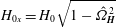 $H_{0x}=H_{0}\sqrt{1-\hat{\unicode[STIX]{x1D6FA}}_{\boldsymbol{H}}^{2}}$
. The following scaled equation is obtained when the torque balance equation is divided by
 $4\unicode[STIX]{x03C0}\unicode[STIX]{x1D702}R^{3}|\unicode[STIX]{x1D74E}|$
,
 $$\begin{eqnarray}\displaystyle \frac{\hat{\unicode[STIX]{x1D74E}}\boldsymbol{\cdot }(\hat{\unicode[STIX]{x1D734}}\boldsymbol{\times }\hat{\boldsymbol{H}})}{\sqrt{1-\hat{\unicode[STIX]{x1D6FA}}_{\boldsymbol{H}}^{2}}}-\unicode[STIX]{x1D6F4}\hat{\unicode[STIX]{x1D6FA}}_{\boldsymbol{H}}\sqrt{1-\hat{\unicode[STIX]{x1D6FA}}_{\boldsymbol{H}}^{2}}M_{R}(\unicode[STIX]{x1D6FD}\unicode[STIX]{x1D6FA}^{\ast })=0. & & \displaystyle\end{eqnarray}$$
The functions
 $M_{R}(\unicode[STIX]{x1D6FD}\unicode[STIX]{x1D6FA}^{\ast })$
and
 $M_{I}(\unicode[STIX]{x1D6FD}\unicode[STIX]{x1D6FA}^{\ast })$
are dimensionless functions proportional to the real and imaginary parts of the induced magnetic dipole moment of the particle which are derived in appendix A. In (A 28) and (A 29) for a uniform particle,
 $M_{R}$
and
 $M_{I}$
are functions of the product of the angular velocity scaled by the characteristic relaxation time for the eddy current,
 $\unicode[STIX]{x1D6FA}^{\dagger }=(\unicode[STIX]{x1D707}_{0}\unicode[STIX]{x1D6FA}R^{2}/\unicode[STIX]{x1D71A})$
, where
 $\unicode[STIX]{x1D71A}$
is the electrical resistivity of the particle. Using the substitution
 $\unicode[STIX]{x1D6FA}^{\dagger }=\unicode[STIX]{x1D6FD}_{p}\unicode[STIX]{x1D6FA}^{\ast }$
, where
 $\unicode[STIX]{x1D6FD}_{p}=(|\unicode[STIX]{x1D74E}|\unicode[STIX]{x1D707}_{0}R^{2}/2\unicode[STIX]{x1D71A})$
, the functions
 $M_{R}(\unicode[STIX]{x1D6FD}_{p}\unicode[STIX]{x1D6FA}^{\ast })$
and
 $M_{I}(\unicode[STIX]{x1D6FD}_{p}\unicode[STIX]{x1D6FA}^{\ast })$
are,
 $$\begin{eqnarray}\displaystyle & \displaystyle M_{R}=-\frac{1}{2}+\frac{3}{2\sqrt{2\unicode[STIX]{x1D6FD}_{p}\unicode[STIX]{x1D6FA}^{\ast }}}\frac{\sinh \left(\sqrt{2\unicode[STIX]{x1D6FD}_{p}\unicode[STIX]{x1D6FA}^{\ast }}\right)-\sin \left(\sqrt{2\unicode[STIX]{x1D6FD}_{p}\unicode[STIX]{x1D6FA}^{\ast }}\right)}{\cosh \left(\sqrt{2\unicode[STIX]{x1D6FD}_{p}\unicode[STIX]{x1D6FA}^{\ast }}\right)-\cos \left(\sqrt{2\unicode[STIX]{x1D6FD}_{p}\unicode[STIX]{x1D6FA}^{\ast }}\right)}, & \displaystyle\end{eqnarray}$$
 $$\begin{eqnarray}\displaystyle & \displaystyle M_{I}=-\frac{3}{2\unicode[STIX]{x1D6FD}_{p}\unicode[STIX]{x1D6FA}^{\ast }}+\frac{3}{2\sqrt{2\unicode[STIX]{x1D6FD}_{p}\unicode[STIX]{x1D6FA}^{\ast }}}\frac{\sinh \left(\sqrt{2\unicode[STIX]{x1D6FD}_{p}\unicode[STIX]{x1D6FA}^{\ast }}\right)+\sin \left(\sqrt{2\unicode[STIX]{x1D6FD}_{p}\unicode[STIX]{x1D6FA}^{\ast }}\right)}{\cosh \left(\sqrt{2\unicode[STIX]{x1D6FD}_{p}\unicode[STIX]{x1D6FA}^{\ast }}\right)-\cos \left(\sqrt{2\unicode[STIX]{x1D6FD}_{p}\unicode[STIX]{x1D6FA}^{\ast }}\right)}. & \displaystyle\end{eqnarray}$$
In the limits
 $\unicode[STIX]{x1D6FD}_{p}\unicode[STIX]{x1D6FA}^{\ast }\ll 1$
and
 $\unicode[STIX]{x1D6FD}_{p}\unicode[STIX]{x1D6FA}^{\ast }\gg 1$
, the functions
 $M_{R}$
and
 $M_{I}$
are,
 $$\begin{eqnarray}\displaystyle M_{R} & = & \displaystyle -\frac{(\unicode[STIX]{x1D6FD}_{p}\unicode[STIX]{x1D6FA}^{\ast })^{2}}{315}\quad \text{for }\unicode[STIX]{x1D6FD}_{p}\unicode[STIX]{x1D6FA}^{\ast }\ll 1,\end{eqnarray}$$
 $$\begin{eqnarray}\displaystyle & = & \displaystyle -\frac{1}{2}\quad \text{for }\unicode[STIX]{x1D6FD}_{p}\unicode[STIX]{x1D6FA}^{\ast }\gg 1,\end{eqnarray}$$
 $$\begin{eqnarray}\displaystyle M_{I} & = & \displaystyle \frac{\unicode[STIX]{x1D6FD}_{p}\unicode[STIX]{x1D6FA}^{\ast }}{30}\quad \text{for }\unicode[STIX]{x1D6FD}_{p}\unicode[STIX]{x1D6FA}^{\ast }\ll 1,\end{eqnarray}$$
 $$\begin{eqnarray}\displaystyle & = & \displaystyle \frac{3}{2\sqrt{2\unicode[STIX]{x1D6FD}_{p}\unicode[STIX]{x1D6FA}^{\ast }}}\quad \text{for }\unicode[STIX]{x1D6FD}_{p}\unicode[STIX]{x1D6FA}^{\ast }\gg 1.\end{eqnarray}$$
The functions
 $M_{R}(\unicode[STIX]{x1D6FD}_{p}\unicode[STIX]{x1D6FA}^{\ast })$
and
 $M_{I}(\unicode[STIX]{x1D6FD}_{p}\unicode[STIX]{x1D6FA}^{\ast })$
, along with their limiting behaviour for
 $\unicode[STIX]{x1D6FD}_{p}\unicode[STIX]{x1D6FA}^{\ast }\ll 1$
and
 $\unicode[STIX]{x1D6FD}_{p}\unicode[STIX]{x1D6FA}^{\ast }\gg 1$
, are shown in figure 2(a).
The functions
 $-M_{R}$
(dashed line) and
 $M_{I}$
(solid line) (a) as a function of
 $(\unicode[STIX]{x1D6FD}_{p}\unicode[STIX]{x1D6FA}^{\ast })$
for a uniform particle (equations (2.8) and (2.9)) and (b) as a function of
 $(\unicode[STIX]{x1D6FD}_{s}\unicode[STIX]{x1D6FA}^{\ast })$
for a thin shell (equations (2.14) and (2.15)). The approximations (2.10)–(2.13) in the limits
 $(\unicode[STIX]{x1D6FD}_{p}\unicode[STIX]{x1D6FA}^{\ast })\ll 1$
and
 $(\unicode[STIX]{x1D6FD}_{p}\unicode[STIX]{x1D6FA}^{\ast })\gg 1$
for a uniform particle are shown by the dotted lines in (a), and the equivalent approximations in the limits
 $(\unicode[STIX]{x1D6FD}_{s}\unicode[STIX]{x1D6FA}^{\ast })\ll 1$
and
 $(\unicode[STIX]{x1D6FD}_{s}\unicode[STIX]{x1D6FA}^{\ast })\gg 1$
for a thin shell are shown by the dotted lines in (b).

For a thin shell of radius
 $R$
and thickness
 $R\unicode[STIX]{x1D6FF}$
with
 $\unicode[STIX]{x1D6FF}\ll 1$
, the functions
 $M_{R}$
and
 $M_{I}$
in (A 32)–(A 33) are functions of the scaled frequency
 $\unicode[STIX]{x1D6FA}^{\ddagger }=(\unicode[STIX]{x1D707}_{0}\unicode[STIX]{x1D6FA}R^{2}\unicode[STIX]{x1D6FF}/\unicode[STIX]{x1D71A})$
. Using the substitution
 $\unicode[STIX]{x1D6FA}^{\ddagger }=\unicode[STIX]{x1D6FD}_{s}\unicode[STIX]{x1D6FA}^{\ast }$
where
 $\unicode[STIX]{x1D6FD}_{s}=(|\unicode[STIX]{x1D74E}|\unicode[STIX]{x1D707}_{0}R^{2}\unicode[STIX]{x1D6FF}/2\unicode[STIX]{x1D71A})$
, the functions
 $M_{R}(\unicode[STIX]{x1D6FD}_{s}\unicode[STIX]{x1D6FA}^{\ast })$
and
 $M_{I}(\unicode[STIX]{x1D6FD}_{s}\unicode[STIX]{x1D6FA}^{\ast })$
are,
 $$\begin{eqnarray}\displaystyle & \displaystyle M_{R}=-\frac{(\unicode[STIX]{x1D6FD}_{s}\unicode[STIX]{x1D6FA}^{\ast })^{2}}{2(9+(\unicode[STIX]{x1D6FD}_{s}\unicode[STIX]{x1D6FA}^{\ast })^{2})}, & \displaystyle\end{eqnarray}$$
 $$\begin{eqnarray}\displaystyle & \displaystyle M_{I}=\frac{3\unicode[STIX]{x1D6FD}_{s}\unicode[STIX]{x1D6FA}^{\ast }}{2(9+(\unicode[STIX]{x1D6FD}_{s}\unicode[STIX]{x1D6FA}^{\ast })^{2})}. & \displaystyle\end{eqnarray}$$
Figure 2(b) shows the functions
 $M_{R}(\unicode[STIX]{x1D6FD}_{s}\unicode[STIX]{x1D6FA}^{\ast })$
and
 $M_{I}(\unicode[STIX]{x1D6FD}_{s}\unicode[STIX]{x1D6FA}^{\ast })$
, along with their limiting behaviour for
 $\unicode[STIX]{x1D6FD}_{s}\unicode[STIX]{x1D6FA}^{\ast }\ll 1$
and
 $\unicode[STIX]{x1D6FD}_{s}\unicode[STIX]{x1D6FA}^{\ast }\gg 1$
.
In the present problem, the angular velocity
 $\unicode[STIX]{x1D734}$
has to be determined by setting the total torque equal to zero. Therefore, it is necessary to reframe the equations in terms of the unit vectors
 $\hat{\unicode[STIX]{x1D74E}}$
and
 $\hat{\boldsymbol{H}}$
, instead of
 $\hat{\unicode[STIX]{x1D734}}$
and
 $\hat{\boldsymbol{H}}$
. The three orthonormal unit vectors are
 $\hat{\unicode[STIX]{x1D74E}}$
, (
 $(\hat{\boldsymbol{H}}-\hat{\unicode[STIX]{x1D74E}}(\hat{\unicode[STIX]{x1D74E}}\boldsymbol{\cdot }\hat{\boldsymbol{H}}))/\sqrt{1-(\hat{\unicode[STIX]{x1D74E}}\boldsymbol{\cdot }\hat{\boldsymbol{H}})^{2}}$
) and
 $((\hat{\unicode[STIX]{x1D74E}}\boldsymbol{\times }\hat{\boldsymbol{H}})/\sqrt{1-(\hat{\unicode[STIX]{x1D74E}}\boldsymbol{\cdot }\hat{\boldsymbol{H}})^{2}})$
, and the components of the unit angular velocity vector in these three directions are given by (2.2)–(2.4). The torque balance (2.5)–(2.7) are simplified as follows. Addition of
 $\hat{\unicode[STIX]{x1D6FA}}_{\boldsymbol{H}}$
times (2.5) and
 $\sqrt{1-\hat{\unicode[STIX]{x1D6FA}}_{\boldsymbol{H}}^{2}}$
times (2.6) results in the following equation relating
 $\unicode[STIX]{x1D6FA}^{\ast }$
and
 $\hat{\unicode[STIX]{x1D6FA}}_{\boldsymbol{H}}$
,
 $$\begin{eqnarray}\displaystyle \hat{\unicode[STIX]{x1D74E}}\boldsymbol{\cdot }\hat{\boldsymbol{H}}-\unicode[STIX]{x1D6FA}^{\ast }\hat{\unicode[STIX]{x1D6FA}}_{\boldsymbol{H}}=0. & & \displaystyle\end{eqnarray}$$
This is a general result independent of the dimensionless parameters
 $\unicode[STIX]{x1D6F4}$
and
 $\unicode[STIX]{x1D6FD}$
, and independent of the form of the functions
 $M_{R}$
and
 $M_{I}$
in (2.5)–(2.7). When expressed in dimensional form by multiplying throughout by
 $|\unicode[STIX]{x1D74E}|/2$
, this result states that the projection of the particle angular velocity vector onto the direction of the magnetic field is equal to the projection of fluid rotation rate (one half of the vorticity) onto the direction of the magnetic field. This is because the torque due to the eddy current is always perpendicular to the direction of the applied magnetic field.
Equation (2.16) is inserted into (2.5) and (2.7) to obtain equations for
 $\hat{\unicode[STIX]{x1D6FA}}_{\unicode[STIX]{x1D74E}}$
and
 $\hat{\unicode[STIX]{x1D734}}\boldsymbol{\cdot }((\hat{\unicode[STIX]{x1D74E}}\boldsymbol{\times }\hat{\boldsymbol{H}})/\sqrt{1-(\hat{\unicode[STIX]{x1D74E}}\boldsymbol{\cdot }\hat{\boldsymbol{H}})^{2}})$
,
 $$\begin{eqnarray}\displaystyle & \displaystyle \hat{\unicode[STIX]{x1D6FA}}_{\unicode[STIX]{x1D74E}}=\frac{\hat{\unicode[STIX]{x1D74E}}\boldsymbol{\cdot }\hat{\boldsymbol{H}}}{\hat{\unicode[STIX]{x1D6FA}}_{\boldsymbol{H}}}+\unicode[STIX]{x1D6F4}(1-\hat{\unicode[STIX]{x1D6FA}}_{\boldsymbol{H}}^{2})M_{I}\left(\frac{\unicode[STIX]{x1D6FD}\hat{\unicode[STIX]{x1D74E}}\boldsymbol{\cdot }\hat{\boldsymbol{H}}}{\hat{\unicode[STIX]{x1D6FA}}_{\boldsymbol{H}}}\right), & \displaystyle\end{eqnarray}$$
 $$\begin{eqnarray}\displaystyle & \displaystyle \hat{\unicode[STIX]{x1D6FA}}_{\bot }=\hat{\unicode[STIX]{x1D734}}\boldsymbol{\cdot }\frac{(\hat{\unicode[STIX]{x1D74E}}\boldsymbol{\times }\hat{\boldsymbol{H}})}{\sqrt{1-(\hat{\unicode[STIX]{x1D74E}}\boldsymbol{\cdot }\hat{\boldsymbol{H}})^{2}}}=\text{}-\frac{\unicode[STIX]{x1D6F4}\hat{\unicode[STIX]{x1D6FA}}_{\boldsymbol{H}}(1-\hat{\unicode[STIX]{x1D6FA}}_{\boldsymbol{H}}^{2})}{\sqrt{1-(\hat{\unicode[STIX]{x1D74E}}\boldsymbol{\cdot }\hat{\boldsymbol{H}})^{2}}}M_{R}\left(\frac{\unicode[STIX]{x1D6FD}\hat{\unicode[STIX]{x1D74E}}\boldsymbol{\cdot }\hat{\boldsymbol{H}}}{\hat{\unicode[STIX]{x1D6FA}}_{\boldsymbol{H}}}\right). & \displaystyle\end{eqnarray}$$
Equations (2.17) and (2.18) can be solved for
 $\hat{\unicode[STIX]{x1D6FA}}_{\boldsymbol{H}}$
by realising that
 $\hat{\unicode[STIX]{x1D6FA}}_{\unicode[STIX]{x1D74E}}$
,
 $\hat{\unicode[STIX]{x1D6FA}}_{\Vert }$
and
 $\hat{\unicode[STIX]{x1D6FA}}_{\bot }$
are the components of the unit vector
 $\hat{\unicode[STIX]{x1D734}}$
, and so the sum of the squares of the components is
 $1$
,
 $$\begin{eqnarray}\displaystyle {\hat{\unicode[STIX]{x1D6FA}}_{\unicode[STIX]{x1D74E}}}^{2}+\hat{\unicode[STIX]{x1D6FA}}_{\Vert }^{2}+\hat{\unicode[STIX]{x1D6FA}}_{\bot }^{2}=1. & & \displaystyle\end{eqnarray}$$
In (2.19),
 $\hat{\unicode[STIX]{x1D6FA}}_{\unicode[STIX]{x1D74E}}$
and
 $\hat{\unicode[STIX]{x1D6FA}}_{\Vert }$
are expressed as functions of
 $\hat{\unicode[STIX]{x1D6FA}}_{\boldsymbol{H}}$
and
 $\hat{\unicode[STIX]{x1D74E}}\boldsymbol{\cdot }\hat{\boldsymbol{H}}$
using (2.17), and
 $\hat{\unicode[STIX]{x1D6FA}}_{\bot }$
is expressed as a function of
 $\hat{\unicode[STIX]{x1D6FA}}_{\boldsymbol{H}}$
and
 $\hat{\unicode[STIX]{x1D74E}}\boldsymbol{\cdot }\hat{\boldsymbol{H}}$
using (2.18), to obtain an implicit equation which is solved for
 $\hat{\unicode[STIX]{x1D6FA}}_{\boldsymbol{H}}$
for specified values of
 $\hat{\unicode[STIX]{x1D74E}}\boldsymbol{\cdot }\hat{\boldsymbol{H}}$
,
 $\unicode[STIX]{x1D6F4}$
and
 $\unicode[STIX]{x1D6FD}$
. The solution for
 $\hat{\unicode[STIX]{x1D6FA}}_{\boldsymbol{H}}$
is then substituted into (2.16) to determine
 $\unicode[STIX]{x1D6FA}^{\ast }$
, equation (2.17) to determine
 $\hat{\unicode[STIX]{x1D6FA}}_{\unicode[STIX]{x1D74E}}$
, equation (2.3) to determine
 $\hat{\unicode[STIX]{x1D6FA}}_{\Vert }$
and (2.18) to determine
 $\hat{\unicode[STIX]{x1D6FA}}_{\bot }$
.
Though (2.19) is an implicit equation, it is easy to solve numerically because
 $\hat{\unicode[STIX]{x1D6FA}}_{\boldsymbol{H}}$
is a direction cosine bounded by
 $\pm 1$
. Equation (2.19) provides a solution for
 $\hat{\unicode[STIX]{x1D6FA}}_{\boldsymbol{H}}^{2}$
, rather than
 $\hat{\unicode[STIX]{x1D6FA}}_{\boldsymbol{H}}$
. Due to this, if
 $\hat{\unicode[STIX]{x1D6FA}}_{\boldsymbol{H}}$
is a solution of the equations,
 $-\hat{\unicode[STIX]{x1D6FA}}_{\boldsymbol{H}}$
is also a solution. However, the solutions
 $\pm \hat{\unicode[STIX]{x1D6FA}}_{\boldsymbol{H}}$
also lead to solutions of opposite sign for
 $\unicode[STIX]{x1D6FA}^{\ast }$
in (2.16), resulting in the same solution for the angular velocity vector,
 $\unicode[STIX]{x1D734}^{\ast }=\unicode[STIX]{x1D6FA}^{\ast }\hat{\unicode[STIX]{x1D734}}$
. Since
 $\unicode[STIX]{x1D6FA}^{\ast }$
is the magnitude of the velocity, the sign of
 $\unicode[STIX]{x1D6FA}^{\ast }$
is chosen to be positive, and
 $\hat{\unicode[STIX]{x1D6FA}}_{\boldsymbol{H}}$
has the same sign as
 $\hat{\unicode[STIX]{x1D74E}}\boldsymbol{\cdot }\hat{\boldsymbol{H}}$
.
Upon reversal of sign of
 $\hat{\unicode[STIX]{x1D74E}}\boldsymbol{\cdot }\hat{\boldsymbol{H}}$
, equations (2.17)–(2.19) are satisfied if the sign of
 $\hat{\unicode[STIX]{x1D6FA}}_{\boldsymbol{H}}$
is reversed, the sign of
 $\hat{\unicode[STIX]{x1D6FA}}_{\unicode[STIX]{x1D74E}}$
is unchanged, and the sign of
 $\hat{\unicode[STIX]{x1D6FA}}_{\bot }$
is reversed. This implies that the change in parity
 $\hat{\unicode[STIX]{x1D74E}}\boldsymbol{\cdot }\hat{\boldsymbol{H}}\rightarrow -\hat{\unicode[STIX]{x1D74E}}\boldsymbol{\cdot }\hat{\boldsymbol{H}}$
results in the transformation
 $\hat{\unicode[STIX]{x1D6FA}}_{\boldsymbol{H}}\rightarrow -\hat{\unicode[STIX]{x1D6FA}}_{\boldsymbol{H}}$
,
 $\unicode[STIX]{x1D6FA}^{\ast }\rightarrow \unicode[STIX]{x1D6FA}^{\ast }$
,
 $\hat{\unicode[STIX]{x1D6FA}}_{\unicode[STIX]{x1D74E}}\rightarrow \hat{\unicode[STIX]{x1D6FA}}_{\unicode[STIX]{x1D74E}}$
,
 $\hat{\unicode[STIX]{x1D6FA}}_{\Vert }\rightarrow -\hat{\unicode[STIX]{x1D6FA}}_{\Vert }$
and
 $\hat{\unicode[STIX]{x1D6FA}}_{\bot }\rightarrow -\hat{\unicode[STIX]{x1D6FA}}_{\bot }$
. Therefore, results are restricted to positive
 $\hat{\unicode[STIX]{x1D74E}}\boldsymbol{\cdot }\hat{\boldsymbol{H}}$
, and the results for negative
 $\hat{\unicode[STIX]{x1D74E}}\boldsymbol{\cdot }\hat{\boldsymbol{H}}$
can be determined from symmetry.
3 Stress
The torque exerted on the fluid by a particle
 $i$
is due to the difference between the angular velocity and fluid rotation rate is,
 $$\begin{eqnarray}\displaystyle \boldsymbol{L}_{i}=8\unicode[STIX]{x03C0}\unicode[STIX]{x1D702}R^{3}\unicode[STIX]{x1D734}_{i}^{\prime }, & & \displaystyle\end{eqnarray}$$
where the ‘disturbance’ to the particle angular velocity
 $\unicode[STIX]{x1D734}_{i}^{\prime }$
, which is defined as the difference between the angular velocity and the local fluid angular velocity,
 $$\begin{eqnarray}\displaystyle \unicode[STIX]{x1D734}_{i}^{\prime } & = & \displaystyle (\unicode[STIX]{x1D734}_{i}-\unicode[STIX]{x1D74E}(\boldsymbol{x}_{i})/2)\nonumber\\ \displaystyle & = & \displaystyle \frac{|\unicode[STIX]{x1D74E}(\boldsymbol{x}_{i})|}{2}\left((\unicode[STIX]{x1D6FA}_{i}^{\ast }\hat{\unicode[STIX]{x1D6FA}}_{\unicode[STIX]{x1D74E}i}-1)\hat{\unicode[STIX]{x1D74E}}_{i}+\frac{\unicode[STIX]{x1D6FA}_{i}^{\ast }\hat{\unicode[STIX]{x1D6FA}}_{\Vert i}(\hat{\boldsymbol{H}}_{i}-\hat{\unicode[STIX]{x1D74E}}_{i}(\hat{\unicode[STIX]{x1D74E}}_{i}\boldsymbol{\cdot }\hat{\boldsymbol{H}}_{i}))}{\sqrt{1-(\hat{\unicode[STIX]{x1D74E}}_{i}\boldsymbol{\cdot }\hat{\boldsymbol{H}}_{i})^{2}}}+\frac{\unicode[STIX]{x1D6FA}_{i}^{\ast }\hat{\unicode[STIX]{x1D6FA}}_{\bot i}(\hat{\unicode[STIX]{x1D74E}}_{i}\boldsymbol{\times }\hat{\boldsymbol{H}}_{i})}{\sqrt{1-(\hat{\unicode[STIX]{x1D74E}}_{i}\boldsymbol{\cdot }\hat{\boldsymbol{H}}_{i})^{2}}}\right),\nonumber\\ \displaystyle & & \displaystyle\end{eqnarray}$$
where the subscript
 $i$
indicates that the quantities are evaluated at the centre of particle
 $i$
. The particle stress
 $\unicode[STIX]{x1D748}^{(p)}$
is then given by (Batchelor Reference Batchelor1970),
 $$\begin{eqnarray}\displaystyle \unicode[STIX]{x1D748}^{(p)} & = & \displaystyle \frac{1}{2V}\mathop{\sum }_{i=1}^{N}\hat{\unicode[STIX]{x1D750}}\boldsymbol{ : }\boldsymbol{L}_{i}\nonumber\\ \displaystyle & = & \displaystyle \frac{2\unicode[STIX]{x03C0}\unicode[STIX]{x1D702}R^{3}}{V}\mathop{\sum }_{i=1}^{N}|\unicode[STIX]{x1D74E}(\boldsymbol{x}_{i})|\left((\unicode[STIX]{x1D6FA}_{i}^{\ast }\hat{\unicode[STIX]{x1D6FA}}_{\unicode[STIX]{x1D74E}i}-1)(\hat{\unicode[STIX]{x1D750}}\boldsymbol{ : }\hat{\unicode[STIX]{x1D74E}}_{i})+\frac{\unicode[STIX]{x1D6FA}_{i}^{\ast }\hat{\unicode[STIX]{x1D6FA}}_{\Vert i}\hat{\unicode[STIX]{x1D750}}\mathbf{:}(\hat{\boldsymbol{H}}_{i}-\hat{\unicode[STIX]{x1D74E}}_{i}(\hat{\unicode[STIX]{x1D74E}}_{i}\boldsymbol{\cdot }\hat{\boldsymbol{H}}_{i}))}{\sqrt{1-(\hat{\unicode[STIX]{x1D74E}}_{i}\boldsymbol{\cdot }\hat{\boldsymbol{H}}_{i})^{2}}}\right.\nonumber\\ \displaystyle & & \displaystyle \left.+\,\frac{\unicode[STIX]{x1D6FA}_{i}^{\ast }\hat{\unicode[STIX]{x1D6FA}}_{\bot i}(\hat{\unicode[STIX]{x1D74E}}_{i}\hat{\boldsymbol{H}}_{i}-\hat{\boldsymbol{H}}_{i}\hat{\unicode[STIX]{x1D74E}}_{i})}{\sqrt{1-(\hat{\unicode[STIX]{x1D74E}}_{i}\boldsymbol{\cdot }\hat{\boldsymbol{H}}_{i})^{2}}}\right),\end{eqnarray}$$
where
 $\hat{\unicode[STIX]{x1D750}}$
is the third-order Levi-Civita antisymmetric tensor. The particle stress can now be evaluated if
 $\unicode[STIX]{x1D6FA}_{i}^{\ast }$
,
 $\hat{\unicode[STIX]{x1D6FA}}_{\unicode[STIX]{x1D74E}i}$
,
 $\hat{\unicode[STIX]{x1D6FA}}_{\Vert i}$
and
 $\hat{\unicode[STIX]{x1D6FA}}_{\bot i}$
are determined for specified values of the fluid vorticity and the magnetic field at the particle centre.
The particle stress consists of three antisymmetric components, which are denoted the first and third couple stresses. The first couple stress, proportional to
 $(\unicode[STIX]{x1D6FA}^{\ast }\hat{\unicode[STIX]{x1D6FA}}_{\unicode[STIX]{x1D74E}}-1)$
, is in the plane perpendicular to the vorticity vector. The magnitude of this component is negative, because the eddy current exerts a torque opposite in direction to the particle angular velocity, which tends to slow down the particle rotation rate. For a unidirectional flow in which the vorticity is perpendicular to the flow plane, this results in an antisymmetric component of the stress tensor in the flow plane. The second couple stress, with magnitude
 $\unicode[STIX]{x1D6FA}^{\ast }\hat{\unicode[STIX]{x1D6FA}}_{\Vert }$
, is perpendicular to the unit vector
 $(\hat{\boldsymbol{H}}_{i}-\hat{\unicode[STIX]{x1D74E}}_{i}(\hat{\unicode[STIX]{x1D74E}}\boldsymbol{\cdot }\hat{\boldsymbol{H}}_{i}))/\sqrt{1-(\hat{\unicode[STIX]{x1D74E}}_{i}\boldsymbol{\cdot }\hat{\boldsymbol{H}}_{i})^{2}}$
. The third couple stress with magnitude
 $\unicode[STIX]{x1D6FA}^{\ast }\hat{\unicode[STIX]{x1D6FA}}_{\bot }$
, is in the
 $\hat{\unicode[STIX]{x1D74E}}_{i}{-}\hat{\boldsymbol{H}}_{i}$
plane.
In a dilute suspension where the fluid vorticity is independent of position and particle interactions are neglected, all the particles in the suspension rotate with equal angular velocity and the quantities
 $\unicode[STIX]{x1D6FA}^{\ast }$
,
 $\hat{\unicode[STIX]{x1D6FA}}_{\unicode[STIX]{x1D74E}}$
,
 $\hat{\unicode[STIX]{x1D6FA}}_{\Vert }$
and
 $\hat{\unicode[STIX]{x1D6FA}}_{\bot }$
are independent of position. The particle stress is,
 $$\begin{eqnarray}\displaystyle \unicode[STIX]{x1D748}^{(p)}=|\unicode[STIX]{x1D74E}|\left(\unicode[STIX]{x1D702}_{c}^{(1)}(\hat{\unicode[STIX]{x1D750}}\boldsymbol{ : }\hat{\unicode[STIX]{x1D74E}})+\frac{\unicode[STIX]{x1D702}_{c}^{(2)}\hat{\unicode[STIX]{x1D750}}\mathbf{:}(\hat{\boldsymbol{H}}-\hat{\unicode[STIX]{x1D74E}}(\hat{\unicode[STIX]{x1D74E}}\boldsymbol{\cdot }\hat{\boldsymbol{H}}))}{\sqrt{1-(\hat{\unicode[STIX]{x1D74E}}\boldsymbol{\cdot }\hat{\boldsymbol{H}})^{2}}}+\frac{\unicode[STIX]{x1D702}_{c}^{(3)}(\hat{\unicode[STIX]{x1D74E}}\hat{\boldsymbol{H}}-\hat{\boldsymbol{H}}\hat{\unicode[STIX]{x1D74E}})}{\sqrt{1-(\hat{\unicode[STIX]{x1D74E}}\boldsymbol{\cdot }\hat{\boldsymbol{H}})^{2}}}\right), & & \displaystyle\end{eqnarray}$$
where the three couple stress coefficients are,
 $$\begin{eqnarray}\displaystyle & \displaystyle \unicode[STIX]{x1D702}_{c}^{(1)}=\frac{3\unicode[STIX]{x1D719}\unicode[STIX]{x1D702}(\unicode[STIX]{x1D6FA}^{\ast }\hat{\unicode[STIX]{x1D6FA}}_{\unicode[STIX]{x1D74E}}-1)}{2}, & \displaystyle\end{eqnarray}$$
 $$\begin{eqnarray}\displaystyle & \displaystyle \unicode[STIX]{x1D702}_{c}^{(2)}=\frac{3\unicode[STIX]{x1D719}\unicode[STIX]{x1D702}\unicode[STIX]{x1D6FA}^{\ast }\hat{\unicode[STIX]{x1D6FA}}_{\Vert }}{2}, & \displaystyle\end{eqnarray}$$
 $$\begin{eqnarray}\displaystyle & \displaystyle \unicode[STIX]{x1D702}_{c}^{(3)}=\frac{3\unicode[STIX]{x1D719}\unicode[STIX]{x1D702}\unicode[STIX]{x1D6FA}^{\ast }\hat{\unicode[STIX]{x1D6FA}}_{\bot }}{2}. & \displaystyle\end{eqnarray}$$
The first and second couple stress coefficients are related due to the condition that the component of the torque in the direction of the magnetic field is zero. Equation (2.16) can be used to simplify (2.3) for
 $\hat{\unicode[STIX]{x1D6FA}}_{\Vert }$
,
 $$\begin{eqnarray}\displaystyle \hat{\unicode[STIX]{x1D6FA}}_{\Vert }=\frac{\hat{\unicode[STIX]{x1D74E}}\boldsymbol{\cdot }\hat{\boldsymbol{H}}}{\unicode[STIX]{x1D6FA}^{\ast }\sqrt{1-(\hat{\unicode[STIX]{x1D74E}}\boldsymbol{\cdot }\hat{\boldsymbol{H}})^{2}}}-\frac{\hat{\unicode[STIX]{x1D6FA}}_{\unicode[STIX]{x1D74E}}\hat{\unicode[STIX]{x1D74E}}\boldsymbol{\cdot }\hat{\boldsymbol{H}}}{\sqrt{1-(\hat{\unicode[STIX]{x1D74E}}\boldsymbol{\cdot }\hat{\boldsymbol{H}})^{2}}}. & & \displaystyle\end{eqnarray}$$
When this is multiplied by
 $\unicode[STIX]{x1D6FA}^{\ast }$
, we obtain,
 $$\begin{eqnarray}\displaystyle \unicode[STIX]{x1D6FA}^{\ast }\hat{\unicode[STIX]{x1D6FA}}_{\Vert }=\frac{\hat{\unicode[STIX]{x1D74E}}\boldsymbol{\cdot }\hat{\boldsymbol{H}}}{\sqrt{1-(\hat{\unicode[STIX]{x1D74E}}\boldsymbol{\cdot }\hat{\boldsymbol{H}})^{2}}}\left(1-\unicode[STIX]{x1D6FA}^{\ast }\hat{\unicode[STIX]{x1D6FA}}_{\unicode[STIX]{x1D74E}}\right). & & \displaystyle\end{eqnarray}$$
Comparing (3.5), (3.6) and (3.9), the following relation is obtained between the couple stress coefficients
 $\unicode[STIX]{x1D702}_{c}^{(1)}$
and
 $\unicode[STIX]{x1D702}_{c}^{(2)}$
,
 $$\begin{eqnarray}\displaystyle \unicode[STIX]{x1D702}_{c}^{(2)}=-\frac{\hat{\unicode[STIX]{x1D74E}}\boldsymbol{\cdot }\hat{\boldsymbol{H}}\unicode[STIX]{x1D702}_{c}^{(1)}}{\sqrt{1-(\hat{\unicode[STIX]{x1D74E}}\boldsymbol{\cdot }\hat{\boldsymbol{H}})^{2}}}. & & \displaystyle\end{eqnarray}$$
It should be noted that (3.10) applies even if the particle angular velocities and magnetic field are not uniform, since the relation (3.9) applies for each individual particle. Results are presented only for the couple stress coefficients
 $\unicode[STIX]{x1D702}_{c}^{(1)}$
and
 $\unicode[STIX]{x1D702}_{c}^{(3)}$
; the coefficient
 $\unicode[STIX]{x1D702}_{c}^{(2)}$
can be determined using (3.10).
4 Oblique magnetic field
Equations (2.17)–(2.19) depend on two dimensionless parameters,
 $\unicode[STIX]{x1D6F4}$
, the ratio of the characteristic magnetic and viscous torque on the particle, and
 $\unicode[STIX]{x1D6FD}$
, the product of the eddy current relaxation time and the vorticity. Equations (2.17)–(2.19) cannot be solved analytically. Therefore, asymptotic solutions are first presented for the limits of small magnetic field
 $(\unicode[STIX]{x1D6F4}\ll 1)$
and large magnetic field
 $(\unicode[STIX]{x1D6F4}\gg 1)$
. For
 $\unicode[STIX]{x1D6F4}\ll 1$
, it is expected that the angular velocity is close to one half of the vorticity, and the correction to the angular velocity is
 $O(\unicode[STIX]{x1D6F4})$
. For
 $\unicode[STIX]{x1D6F4}\gg 1$
, it is shown that the angular velocity aligns with the magnetic field in the leading approximation.
4.1
 $\unicode[STIX]{x1D6F4}\ll 1$

A regular perturbation expansion in the parameter
 $\unicode[STIX]{x1D6F4}$
can be used in (2.5)–(2.7) to obtain,
 $$\begin{eqnarray}\displaystyle \unicode[STIX]{x1D6FA}^{\ast } & = & \displaystyle 1-\unicode[STIX]{x1D6F4}(1-(\hat{\unicode[STIX]{x1D74E}}\boldsymbol{\cdot }\hat{\boldsymbol{H}})^{2})M_{I}(\unicode[STIX]{x1D6FD})+{\textstyle \frac{1}{2}}\unicode[STIX]{x1D6F4}^{2}(1-(\hat{\unicode[STIX]{x1D74E}}\boldsymbol{\cdot }\hat{\boldsymbol{H}})^{2})\nonumber\\ \displaystyle & & \displaystyle \times \,[2M_{I}(\unicode[STIX]{x1D6FD})M_{I}^{\prime }(1-(\hat{\unicode[STIX]{x1D74E}}\boldsymbol{\cdot }\hat{\boldsymbol{H}})^{2})+(\hat{\unicode[STIX]{x1D74E}}\boldsymbol{\cdot }\hat{\boldsymbol{H}})^{2}(3(M_{I}(\unicode[STIX]{x1D6FD}))^{2}-(M_{R}(\unicode[STIX]{x1D6FD}))^{2})]\end{eqnarray}$$
 $$\begin{eqnarray}\hat{\unicode[STIX]{x1D6FA}}_{\unicode[STIX]{x1D74E}}=1-{\textstyle \frac{1}{2}}\unicode[STIX]{x1D6F4}^{2}(\hat{\unicode[STIX]{x1D74E}}\boldsymbol{\cdot }\hat{\boldsymbol{H}})^{2}(1-(\hat{\unicode[STIX]{x1D74E}}\boldsymbol{\cdot }\hat{\boldsymbol{H}})^{2})(M_{R}(\unicode[STIX]{x1D6FD})^{2}+M_{I}(\unicode[STIX]{x1D6FD})^{2})\end{eqnarray}$$
 $$\begin{eqnarray}\displaystyle \hat{\unicode[STIX]{x1D6FA}}_{\Vert } & = & \displaystyle \hat{\unicode[STIX]{x1D74E}}\boldsymbol{\cdot }\hat{\boldsymbol{H}}\sqrt{1-(\hat{\unicode[STIX]{x1D74E}}\boldsymbol{\cdot }\hat{\boldsymbol{H}})^{2}}\left\{\unicode[STIX]{x1D6F4}M_{I}(\unicode[STIX]{x1D6FD})\right.+\unicode[STIX]{x1D6F4}^{2}\left[M_{I}\right.(\unicode[STIX]{x1D6FD})^{2}(1-2(\hat{\unicode[STIX]{x1D74E}}\boldsymbol{\cdot }\hat{\boldsymbol{H}})^{2})\nonumber\\ \displaystyle & & \displaystyle -\,M_{I}(\unicode[STIX]{x1D6FD})M_{I}^{\prime }(1-(\hat{\unicode[STIX]{x1D74E}}\boldsymbol{\cdot }\hat{\boldsymbol{H}})^{2})+(\hat{\unicode[STIX]{x1D74E}}\boldsymbol{\cdot }\hat{\boldsymbol{H}})^{2}M_{R}(\unicode[STIX]{x1D6FD})^{2}\left.\left.\!\!\right]\right\}\end{eqnarray}$$
 $$\begin{eqnarray}\displaystyle \hat{\unicode[STIX]{x1D6FA}}_{\bot } & = & \displaystyle (\hat{\unicode[STIX]{x1D74E}}\boldsymbol{\cdot }\hat{\boldsymbol{H}})\sqrt{1-(\hat{\unicode[STIX]{x1D74E}}\boldsymbol{\cdot }\hat{\boldsymbol{H}})^{2}}\left\{-\unicode[STIX]{x1D6F4}M_{R}(\unicode[STIX]{x1D6FD})\right.+\unicode[STIX]{x1D6F4}^{2}M_{I}(\unicode[STIX]{x1D6FD})\nonumber\\ \displaystyle & & \displaystyle \times [(3(\hat{\unicode[STIX]{x1D74E}}\boldsymbol{\cdot }\hat{\boldsymbol{H}})^{2}-1)M_{R}(\unicode[STIX]{x1D6FD})+(1-(\hat{\unicode[STIX]{x1D74E}}\boldsymbol{\cdot }\hat{\boldsymbol{H}})^{2})M_{R}^{\prime }]\left.\!\!\right\},\end{eqnarray}$$
where
 $$\begin{eqnarray}\displaystyle & \displaystyle M_{R}^{\prime }=\left.\frac{\text{d}M_{R}(\unicode[STIX]{x1D6FD}\unicode[STIX]{x1D6FA}^{\ast })}{\text{d}\unicode[STIX]{x1D6FA}^{\ast }}\right|_{\unicode[STIX]{x1D6FA}^{\ast }=1}, & \displaystyle\end{eqnarray}$$
 $$\begin{eqnarray}\displaystyle & \displaystyle M_{I}^{\prime }=\left.\frac{\text{d}M_{I}(\unicode[STIX]{x1D6FD}\unicode[STIX]{x1D6FA}^{\ast })}{\text{d}\unicode[STIX]{x1D6FA}^{\ast }}\right|_{\unicode[STIX]{x1D6FA}^{\ast }=1}. & \displaystyle\end{eqnarray}$$
The couple stress coefficients are obtained by substituting the solutions (4.1)–(4.4), into (3.5)–(3.7),
 $$\begin{eqnarray}\displaystyle \frac{\unicode[STIX]{x1D702}_{c}^{(1)}}{(3\unicode[STIX]{x1D719}\unicode[STIX]{x1D702}/2)} & = & \displaystyle -\unicode[STIX]{x1D6F4}(1-(\hat{\unicode[STIX]{x1D74E}}\boldsymbol{\cdot }\hat{\boldsymbol{H}})^{2})M_{I}(\unicode[STIX]{x1D6FD})+\unicode[STIX]{x1D6F4}^{2}\left[\right.\!(\hat{\unicode[STIX]{x1D74E}}\boldsymbol{\cdot }\hat{\boldsymbol{H}})^{2}(1-(\hat{\unicode[STIX]{x1D74E}}\boldsymbol{\cdot }\hat{\boldsymbol{H}})^{2})(M_{I}(\unicode[STIX]{x1D6FD})^{2}-M_{R}(\unicode[STIX]{x1D6FD})^{2})\nonumber\\ \displaystyle & & \displaystyle +\,(1-(\hat{\unicode[STIX]{x1D74E}}\boldsymbol{\cdot }\hat{\boldsymbol{H}})^{2})^{2}M_{I}(\unicode[STIX]{x1D6FD})M_{I}^{\prime }\left.\!\right],\end{eqnarray}$$
 $$\begin{eqnarray}\displaystyle \frac{\unicode[STIX]{x1D702}_{c}^{(3)}}{(3\unicode[STIX]{x1D719}\unicode[STIX]{x1D702}/2)} & = & \displaystyle -\unicode[STIX]{x1D6F4}\hat{\unicode[STIX]{x1D74E}}\boldsymbol{\cdot }\hat{\boldsymbol{H}}\sqrt{1-(\hat{\unicode[STIX]{x1D74E}}\boldsymbol{\cdot }\hat{\boldsymbol{H}})^{2}}M_{R}(\unicode[STIX]{x1D6FD})\nonumber\\ \displaystyle & & \displaystyle +\,\unicode[STIX]{x1D6F4}^{2}\left[2\right.\!(\hat{\unicode[STIX]{x1D74E}}\boldsymbol{\cdot }\hat{\boldsymbol{H}})^{3}\sqrt{1-(\hat{\unicode[STIX]{x1D74E}}\boldsymbol{\cdot }\hat{\boldsymbol{H}})^{2}}M_{R}(\unicode[STIX]{x1D6FD})M_{I}(\unicode[STIX]{x1D6FD})\nonumber\\ \displaystyle & & \displaystyle +\,\hat{\unicode[STIX]{x1D74E}}\boldsymbol{\cdot }\hat{\boldsymbol{H}}(1-(\hat{\unicode[STIX]{x1D74E}}\boldsymbol{\cdot }\hat{\boldsymbol{H}})^{2})^{3/2}M_{I}(\unicode[STIX]{x1D6FD})M_{R}^{\prime }\left.\!\right].\end{eqnarray}$$
The couple stress coefficients (4.7)–(4.8) can be simplified in the limits
 $\unicode[STIX]{x1D6FD}\ll 1$
and
 $\unicode[STIX]{x1D6FD}\gg 1$
using (2.10)–(2.13) for a uniform particle and (2.14) and (2.15) for a thin shell. The
 $O(\unicode[STIX]{x1D6F4})$
contributions to the couple stress coefficients for
 $\unicode[STIX]{x1D6F4}\ll 1$
are summarised in table 1. These are proportional to the asymptotic expressions for
 $M_{R}(\unicode[STIX]{x1D6FD}_{p})$
and
 $M_{I}(\unicode[STIX]{x1D6FD}_{p})$
in (2.10)–(2.13) for the regime
 $\unicode[STIX]{x1D6FD}_{p}\ll 1$
and
 $\unicode[STIX]{x1D6F4}\ll 1$
and
 $\unicode[STIX]{x1D6FD}_{p}\gg 1$
and
 $\unicode[STIX]{x1D6F4}\ll \unicode[STIX]{x1D6FD}_{p}^{-1/2}$
for uniform particles, where the largest contribution to the couple stress coefficients is due to the
 $O(\unicode[STIX]{x1D6F4})$
term in (4.7)–(4.8). Similarly, for thin shells, the couple stress coefficients are proportional to the asymptotic expressions for (2.14)–(2.15) for
 $\unicode[STIX]{x1D6FD}_{s}\ll 1$
and
 $\unicode[STIX]{x1D6F4}\ll 1$
and
 $\unicode[STIX]{x1D6FD}_{s}\gg 1$
and
 $\unicode[STIX]{x1D6F4}\ll \unicode[STIX]{x1D6FD}_{s}^{-1}$
. In both the aforementioned regimes, the first couple stress coefficient is proportional to
 $(1-(\hat{\unicode[STIX]{x1D74E}}\boldsymbol{\cdot }\hat{\boldsymbol{H}})^{2})$
, and the third couple stress coefficient is proportional to
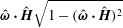 $\hat{\unicode[STIX]{x1D74E}}\boldsymbol{\cdot }\hat{\boldsymbol{H}}\sqrt{1-(\hat{\unicode[STIX]{x1D74E}}\boldsymbol{\cdot }\hat{\boldsymbol{H}})^{2}}$
.


For the first couple stress coefficient, there is an intermediate regime,
 $\unicode[STIX]{x1D6FD}_{p}\gg 1$
and
 $\unicode[STIX]{x1D6F4}\gg \unicode[STIX]{x1D6FD}_{p}^{-1/2}$
for uniform particles and
 $\unicode[STIX]{x1D6FD}_{s}\gg 1$
and
 $\unicode[STIX]{x1D6F4}\gg \unicode[STIX]{x1D6FD}_{s}^{-1}$
for thin shells, where the
 $O(\unicode[STIX]{x1D6F4}^{2})$
term in (4.7) is larger than the
 $O(\unicode[STIX]{x1D6F4})$
term. For a uniform particle,
 $M_{I}(\unicode[STIX]{x1D6FD}_{p})\propto \unicode[STIX]{x1D6FD}_{p}^{-1/2}$
(2.13), and
 $M_{R}(\unicode[STIX]{x1D6FD}_{p})$
tends to
 $-(1/2)$
(2.11). The
 $O(\unicode[STIX]{x1D6F4})$
term on the right in the series in (4.7) is smaller than the
 $O(\unicode[STIX]{x1D6F4}^{2})$
term for
 $(\unicode[STIX]{x1D6F4}/\sqrt{\unicode[STIX]{x1D6FD}_{p}})\ll \unicode[STIX]{x1D6F4}^{2}$
, or
 $\unicode[STIX]{x1D6F4}\gg \unicode[STIX]{x1D6FD}_{p}^{-1/2}$
. For a thin shell,
 $M_{I}(\unicode[STIX]{x1D6FD}_{s})\propto \unicode[STIX]{x1D6FD}_{s}^{-1}$
and
 $M_{R}(\unicode[STIX]{x1D6FD}_{s})=-(1/2)$
for
 $\unicode[STIX]{x1D6FD}_{s}\gg 1$
(equations (2.14)–(2.15)). The
 $O(\unicode[STIX]{x1D6F4})$
term on the right in (4.7) is smaller than the
 $O(\unicode[STIX]{x1D6F4}^{2})$
term for
 $(\unicode[STIX]{x1D6F4}/\unicode[STIX]{x1D6FD}_{s})\ll \unicode[STIX]{x1D6F4}^{2}$
, or
 $\unicode[STIX]{x1D6F4}\gg \unicode[STIX]{x1D6FD}_{s}^{-1}$
. In the two aforementioned regimes, it can be shown that the
 $O(\unicode[STIX]{x1D6F4}^{2})$
term is the largest contribution to the first couple stress coefficient, and this contribution is proportional to
 $(\hat{\unicode[STIX]{x1D74E}}\boldsymbol{\cdot }\hat{\boldsymbol{H}})^{2}(1-(\hat{\unicode[STIX]{x1D74E}}\boldsymbol{\cdot }\hat{\boldsymbol{H}})^{2})$
. The expressions for the first couple stress coefficient in this regime are provided in table 1.
In contrast to the first couple stress coefficient, in (4.8) for the third couple stress coefficient, the
 $O(\unicode[STIX]{x1D6F4})$
term is dominant even for
 $\unicode[STIX]{x1D6FD}_{p}\gg 1$
and
 $\unicode[STIX]{x1D6F4}\gg \unicode[STIX]{x1D6FD}_{p}^{-1/2}$
for a uniform particle and
 $\unicode[STIX]{x1D6FD}_{s}\gg 1$
and
 $\unicode[STIX]{x1D6F4}\gg \unicode[STIX]{x1D6FD}_{s}^{-1}$
for a thin shells. Therefore there is one common expression for the third couple stress coefficient for
 $\unicode[STIX]{x1D6FD}\gg 1$
in table 1.
In table 1, the couple stress coefficients are explicitly expressed in terms of dimensional variables, in order to highlight their vorticity dependence. For
 $\unicode[STIX]{x1D6FD}\ll 1$
, the first and second couple stress coefficients are independent of the magnitude of the vorticity, and the third couple stress coefficient is proportional to the vorticity magnitude
 $|\unicode[STIX]{x1D74E}|$
. Interestingly, for
 $\unicode[STIX]{x1D6FD}\gg 1$
, the couple stress coefficients are proportional to a negative power of the vorticity. The vorticity exponent for the first and third couple stress coefficients is different for uniform particles and thin shells. This is because the high
 $\unicode[STIX]{x1D6FD}$
limit of
 $M_{I}$
for a uniform particle in (2.13) is different from that for a thin shell in (2.15).
4.2
$\unicode[STIX]{x1D6F4}\gg 1$

An examination of (2.5)–(2.7) indicates that
 $(1-\hat{\unicode[STIX]{x1D6FA}}_{\boldsymbol{H}}^{2})$
is necessarily small for
 $\unicode[STIX]{x1D6F4}\gg 1$
, in order to obtain a balance between the terms on the left and right. This implies that the angular velocity is nearly aligned with the magnetic field, and the angle between the two is proportional to
 $\unicode[STIX]{x1D6F4}^{-1}$
for
 $\unicode[STIX]{x1D6F4}\gg 1$
. Expansions for
 $\unicode[STIX]{x1D6FA}^{\ast }$
,
 $\hat{\unicode[STIX]{x1D6FA}}_{\unicode[STIX]{x1D74E}}$
,
 $\hat{\unicode[STIX]{x1D6FA}}_{\Vert }$
and
 $\hat{\unicode[STIX]{x1D6FA}}_{\bot }$
of the form,
 $$\begin{eqnarray}\displaystyle \star =\star ^{(0)}+\unicode[STIX]{x1D6F4}^{-1}\star ^{(1)}+\,\unicode[STIX]{x1D6F4}^{-2}\star ^{(2)}, & & \displaystyle\end{eqnarray}$$
are inserted into the conservation (2.5)–(2.7) and the normalisation condition (2.19). The results, correct to
 $O(\unicode[STIX]{x1D6F4}^{-2})$
, are,
 $$\begin{eqnarray}\unicode[STIX]{x1D6FA}^{\ast }=\hat{\unicode[STIX]{x1D74E}}\boldsymbol{\cdot }\hat{\boldsymbol{H}}+\frac{\unicode[STIX]{x1D6F4}^{-2}(\hat{\unicode[STIX]{x1D74E}}\boldsymbol{\cdot }\hat{\boldsymbol{H}})(1-(\hat{\unicode[STIX]{x1D74E}}\boldsymbol{\cdot }\hat{\boldsymbol{H}})^{2})}{2(M_{I}(\unicode[STIX]{x1D6FD}\hat{\unicode[STIX]{x1D74E}}\boldsymbol{\cdot }\hat{\boldsymbol{H}})^{2}+M_{R}(\unicode[STIX]{x1D6FD}\hat{\unicode[STIX]{x1D74E}}\boldsymbol{\cdot }\hat{\boldsymbol{H}})^{2})},\end{eqnarray}$$
 $$\begin{eqnarray}\displaystyle \hat{\unicode[STIX]{x1D6FA}}_{\unicode[STIX]{x1D74E}} & = & \displaystyle \hat{\unicode[STIX]{x1D74E}}\boldsymbol{\cdot }\hat{\boldsymbol{H}}+\frac{\unicode[STIX]{x1D6F4}^{-1}(1-(\hat{\unicode[STIX]{x1D74E}}\boldsymbol{\cdot }\hat{\boldsymbol{H}})^{2})M_{I}(\unicode[STIX]{x1D6FD}\hat{\unicode[STIX]{x1D74E}}\boldsymbol{\cdot }\hat{\boldsymbol{H}})}{M_{I}(\unicode[STIX]{x1D6FD}\hat{\unicode[STIX]{x1D74E}}\boldsymbol{\cdot }\hat{\boldsymbol{H}})^{2}+M_{R}(\unicode[STIX]{x1D6FD}\hat{\unicode[STIX]{x1D74E}}\boldsymbol{\cdot }\hat{\boldsymbol{H}})^{2}}\nonumber\\ \displaystyle & & \displaystyle +\,\frac{\unicode[STIX]{x1D6F4}^{-2}\hat{\unicode[STIX]{x1D74E}}\boldsymbol{\cdot }\hat{\boldsymbol{H}}(1-(\hat{\unicode[STIX]{x1D74E}}\boldsymbol{\cdot }\hat{\boldsymbol{H}})^{2})}{2(M_{I}(\unicode[STIX]{x1D6FD}\hat{\unicode[STIX]{x1D74E}}\boldsymbol{\cdot }\hat{\boldsymbol{H}})^{2}+M_{R}(\unicode[STIX]{x1D6FD}\hat{\unicode[STIX]{x1D74E}}\boldsymbol{\cdot }\hat{\boldsymbol{H}})^{2})},\end{eqnarray}$$
 $$\begin{eqnarray}\displaystyle \hat{\unicode[STIX]{x1D6FA}}_{\Vert } & = & \displaystyle \sqrt{1-(\hat{\unicode[STIX]{x1D74E}}\boldsymbol{\cdot }\hat{\boldsymbol{H}})^{2}}-\frac{\unicode[STIX]{x1D6F4}^{-1}\hat{\unicode[STIX]{x1D74E}}\boldsymbol{\cdot }\hat{\boldsymbol{H}}\sqrt{1-(\hat{\unicode[STIX]{x1D74E}}\boldsymbol{\cdot }\hat{\boldsymbol{H}})^{2}}M_{I}(\unicode[STIX]{x1D6FD}\hat{\unicode[STIX]{x1D74E}}\boldsymbol{\cdot }\hat{\boldsymbol{H}})}{M_{I}(\unicode[STIX]{x1D6FD}\hat{\unicode[STIX]{x1D74E}}\boldsymbol{\cdot }\hat{\boldsymbol{H}})^{2}+M_{R}(\unicode[STIX]{x1D6FD}\hat{\unicode[STIX]{x1D74E}}\boldsymbol{\cdot }\hat{\boldsymbol{H}})^{2}}\nonumber\\ \displaystyle & & \displaystyle -\,\frac{\unicode[STIX]{x1D6F4}^{-2}\sqrt{1-(\hat{\unicode[STIX]{x1D74E}}\boldsymbol{\cdot }\hat{\boldsymbol{H}})^{2}}(1+(\hat{\unicode[STIX]{x1D74E}}\boldsymbol{\cdot }\hat{\boldsymbol{H}})^{2})}{2(M_{I}(\unicode[STIX]{x1D6FD}\hat{\unicode[STIX]{x1D74E}}\boldsymbol{\cdot }\hat{\boldsymbol{H}})^{2}+M_{R}(\unicode[STIX]{x1D6FD}\hat{\unicode[STIX]{x1D74E}}\boldsymbol{\cdot }\hat{\boldsymbol{H}})^{2})},\end{eqnarray}$$
 $$\begin{eqnarray}\hat{\unicode[STIX]{x1D6FA}}_{\bot }=-\frac{\unicode[STIX]{x1D6F4}^{-1}\sqrt{1-(\hat{\unicode[STIX]{x1D74E}}\boldsymbol{\cdot }\hat{\boldsymbol{H}})^{2}}M_{R}(\unicode[STIX]{x1D6FD}\hat{\unicode[STIX]{x1D74E}}\boldsymbol{\cdot }\hat{\boldsymbol{H}})}{M_{I}(\unicode[STIX]{x1D6FD}\hat{\unicode[STIX]{x1D74E}}\boldsymbol{\cdot }\hat{\boldsymbol{H}})^{2}+M_{R}(\unicode[STIX]{x1D6FD}\hat{\unicode[STIX]{x1D74E}}\boldsymbol{\cdot }\hat{\boldsymbol{H}})^{2}}.\end{eqnarray}$$
Since the angular velocity is nearly aligned with the magnetic field for
 $\unicode[STIX]{x1D6F4}\gg 1$
, the components
 $\hat{\unicode[STIX]{x1D6FA}}_{\unicode[STIX]{x1D74E}}$
and
 $\hat{\unicode[STIX]{x1D6FA}}_{\Vert }$
differ from
 $\hat{\unicode[STIX]{x1D74E}}\boldsymbol{\cdot }\hat{\boldsymbol{H}}$
and
 $\sqrt{1-(\hat{\unicode[STIX]{x1D74E}}\boldsymbol{\cdot }\hat{\boldsymbol{H}})^{2}}$
respectively by
 $O(\unicode[STIX]{x1D6F4}^{-1})$
. The magnitude of the angular velocity tends to
 $\hat{\unicode[STIX]{x1D74E}}\boldsymbol{\cdot }\hat{\boldsymbol{H}}$
in the limit
 $\unicode[STIX]{x1D6F4}\gg 1$
; the difference
 $(\unicode[STIX]{x1D6FA}^{\ast }-\hat{\unicode[STIX]{x1D74E}}\boldsymbol{\cdot }\hat{\boldsymbol{H}})$
is proportional to
 $\unicode[STIX]{x1D6F4}^{-2}$
. The component
 $\hat{\unicode[STIX]{x1D6FA}}_{\bot }$
of the angular velocity unit vector perpendicular to the
 $\hat{\unicode[STIX]{x1D74E}}{-}\hat{\boldsymbol{H}}$
plane is
 $O(\unicode[STIX]{x1D6F4}^{-1})$
. The first and third couple stress coefficients, obtained by substituting the expressions (4.10)–(4.13) into (3.5)–(3.7), are,
 $$\begin{eqnarray}\displaystyle \frac{\unicode[STIX]{x1D702}_{c}^{(1)}}{(3\unicode[STIX]{x1D719}\unicode[STIX]{x1D702}/2)}=-(1-(\hat{\unicode[STIX]{x1D74E}}\boldsymbol{\cdot }\hat{\boldsymbol{H}})^{2})+\frac{\hat{\unicode[STIX]{x1D74E}}\boldsymbol{\cdot }\hat{\boldsymbol{H}}(1-(\hat{\unicode[STIX]{x1D74E}}\boldsymbol{\cdot }\hat{\boldsymbol{H}})^{2})M_{I}(\unicode[STIX]{x1D6FD}\hat{\unicode[STIX]{x1D74E}}\boldsymbol{\cdot }\hat{\boldsymbol{H}})}{\unicode[STIX]{x1D6F4}(M_{R}(\unicode[STIX]{x1D6FD}\hat{\unicode[STIX]{x1D74E}}\boldsymbol{\cdot }\hat{\boldsymbol{H}})^{2}+M_{I}(\unicode[STIX]{x1D6FD}\hat{\unicode[STIX]{x1D74E}}\boldsymbol{\cdot }\hat{\boldsymbol{H}})^{2})}, & & \displaystyle\end{eqnarray}$$
 $$\begin{eqnarray}\displaystyle \frac{\unicode[STIX]{x1D702}_{c}^{(3)}}{(3\unicode[STIX]{x1D719}\unicode[STIX]{x1D702}/2)}=-\frac{\hat{\unicode[STIX]{x1D74E}}\boldsymbol{\cdot }\hat{\boldsymbol{H}}\sqrt{1-(\hat{\unicode[STIX]{x1D74E}}\boldsymbol{\cdot }\hat{\boldsymbol{H}})^{2}}M_{R}(\unicode[STIX]{x1D6FD}\hat{\unicode[STIX]{x1D74E}}\boldsymbol{\cdot }\hat{\boldsymbol{H}})}{\unicode[STIX]{x1D6F4}(M_{R}(\unicode[STIX]{x1D6FD}\hat{\unicode[STIX]{x1D74E}}\boldsymbol{\cdot }\hat{\boldsymbol{H}})^{2}+M_{I}(\unicode[STIX]{x1D6FD}\hat{\unicode[STIX]{x1D74E}}\boldsymbol{\cdot }\hat{\boldsymbol{H}})^{2})}. & & \displaystyle\end{eqnarray}$$
Equation (4.14) indicates that the scaled first couple stress coefficient,
 $(\unicode[STIX]{x1D702}_{c}^{(1)}/(3\unicode[STIX]{x1D719}\unicode[STIX]{x1D702}/2))$
, attains a constant value
 $-(1-(\hat{\unicode[STIX]{x1D74E}}\boldsymbol{\cdot }\hat{\boldsymbol{H}})^{2})$
for
 $\unicode[STIX]{x1D6F4}\gg 1$
; from (3.10), the scaled couple stress coefficient
 $(\unicode[STIX]{x1D702}_{c}^{(2)}/(3\unicode[STIX]{x1D719}\unicode[STIX]{x1D702}/2))$
approaches
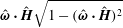 $\hat{\unicode[STIX]{x1D74E}}\boldsymbol{\cdot }\hat{\boldsymbol{H}}\sqrt{1-(\hat{\unicode[STIX]{x1D74E}}\boldsymbol{\cdot }\hat{\boldsymbol{H}})^{2}}$
in this limit. The third couple stress coefficient decreases proportional to
 $\unicode[STIX]{x1D6F4}^{-1}$
for
 $\unicode[STIX]{x1D6F4}\gg 1$
.
The asymptotic limits for the couple stress coefficients for
 $\unicode[STIX]{x1D6FD}\ll 1$
and
 $\unicode[STIX]{x1D6FD}\gg 1$
are listed in table 2. For a thin shell, by coincidence, the asymptotic expressions in the limits
 $\unicode[STIX]{x1D6FD}_{s}\ll 1$
and
 $\unicode[STIX]{x1D6FD}_{s}\gg 1$
are identical, even though the functions
 $M_{R}(\unicode[STIX]{x1D6FD}_{s}\hat{\unicode[STIX]{x1D74E}}\boldsymbol{\cdot }\hat{\boldsymbol{H}})$
and
 $M_{I}(\unicode[STIX]{x1D6FD}_{s}\hat{\unicode[STIX]{x1D74E}}\boldsymbol{\cdot }\hat{\boldsymbol{H}})$
in (4.14)–(4.15) are different. For a uniform particle, the third couple stress coefficient is proportional to
 $\unicode[STIX]{x1D6F4}^{-1}$
and independent of
 $\unicode[STIX]{x1D6FD}_{p}$
for both small and large
 $\unicode[STIX]{x1D6FD}_{p}$
, although there is a small difference in the numerical prefactor. The first couple stress coefficient is independent of
 $|\unicode[STIX]{x1D74E}|$
and the third couple stress coefficient is proportional to
 $|\unicode[STIX]{x1D74E}|$
for a thin shell for small and large
 $\unicode[STIX]{x1D6FD}_{s}$
. For a uniform particle, the third couple stress coefficient is proportional to
 $|\unicode[STIX]{x1D74E}|$
for small and large
 $\unicode[STIX]{x1D6FD}_{p}$
.


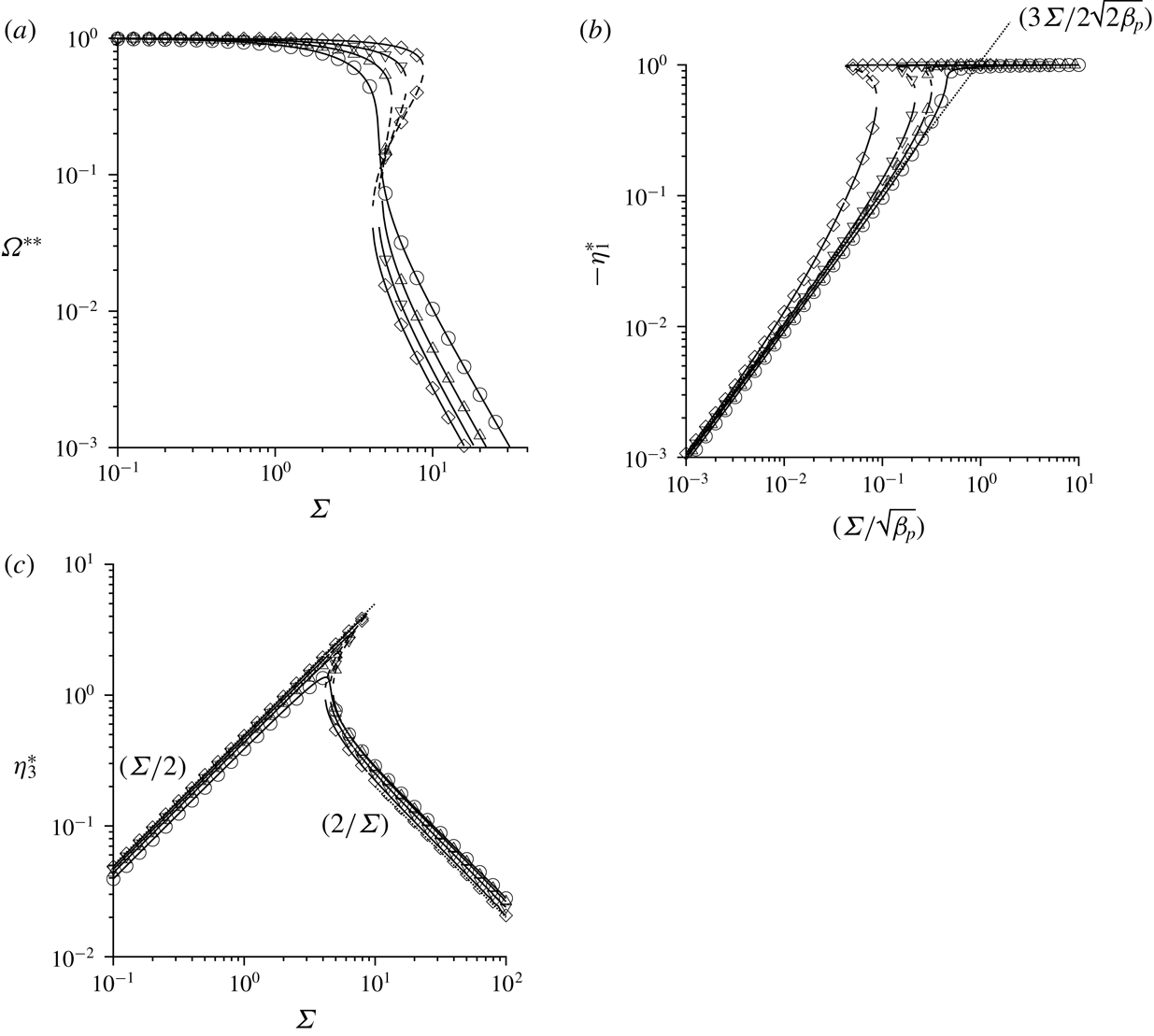
The scaled angular velocity
 $\unicode[STIX]{x1D6FA}^{\ast \ast }$
(a), negative of the scaled first couple stress coefficient
 $-\unicode[STIX]{x1D702}_{1}^{\ast }$
(b) and third couple stress coefficient
 $\unicode[STIX]{x1D702}_{3}^{\ast }$
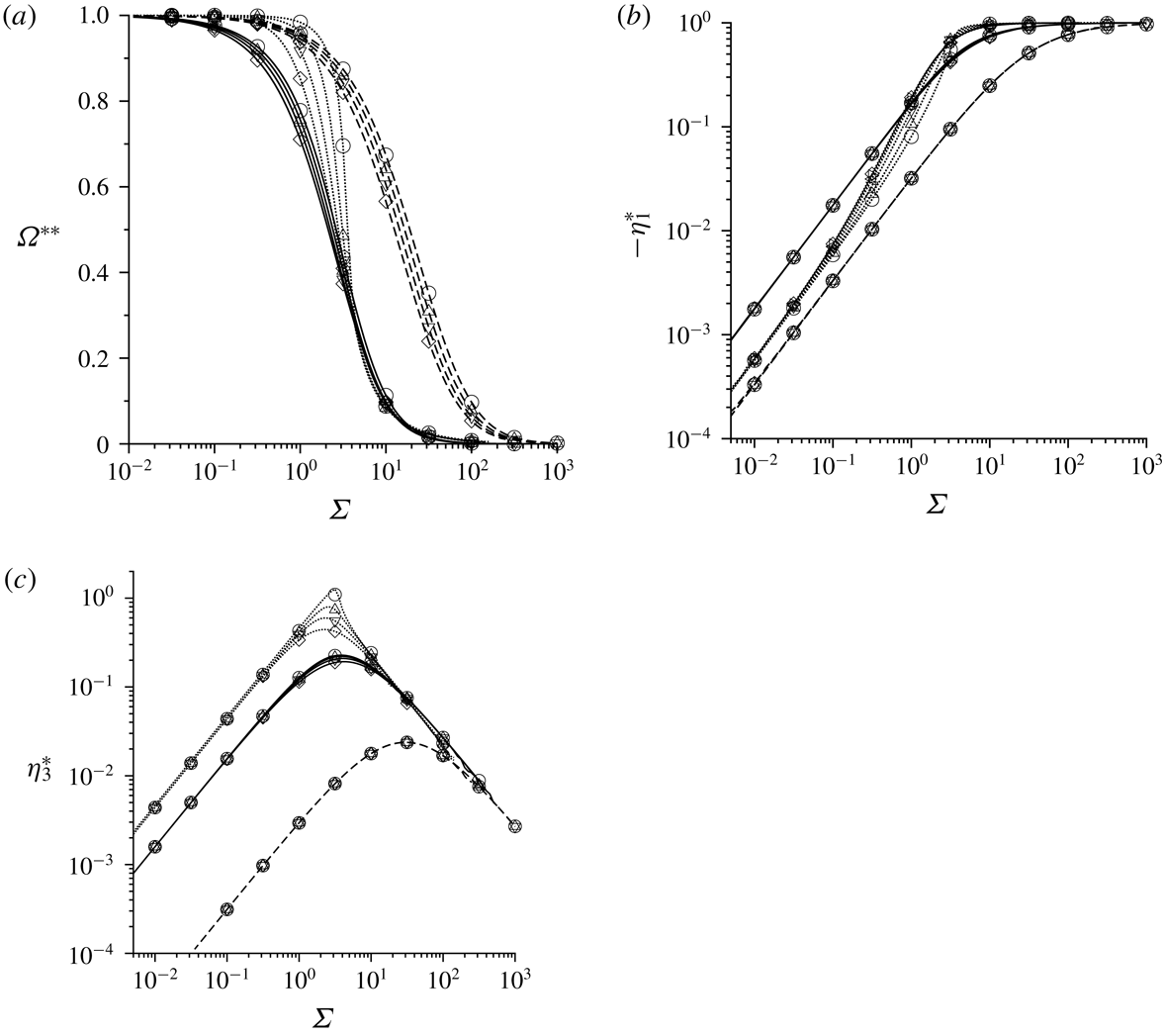
(c), defined in (4.16)–(4.18), as a function of
 $\unicode[STIX]{x1D6F4}$
for a uniform particle with
 $\unicode[STIX]{x1D6FD}_{p}=1$
(dashed lines),
 $\unicode[STIX]{x1D6FD}_{p}=10$
(solid lines) and
 $\unicode[STIX]{x1D6FD}_{p}=1000$
(dotted lines) for ○
 $\hat{\unicode[STIX]{x1D74E}}\boldsymbol{\cdot }\hat{\boldsymbol{H}}=(1/3)$
, ▵
 $\hat{\unicode[STIX]{x1D74E}}\boldsymbol{\cdot }\hat{\boldsymbol{H}}=(1/2)$
, ▿
 $\hat{\unicode[STIX]{x1D74E}}\boldsymbol{\cdot }\hat{\boldsymbol{H}}=(1/\sqrt{2})$
and ♢
 $\hat{\unicode[STIX]{x1D74E}}\boldsymbol{\cdot }\hat{\boldsymbol{H}}=0.99$
.

4.3 Numerical results
The variation of the scaled particle angular velocity and couple stress coefficients with
 $\unicode[STIX]{x1D6F4}$
for different values of
 $\unicode[STIX]{x1D6FD}$
and
 $\hat{\unicode[STIX]{x1D74E}}\boldsymbol{\cdot }\hat{\boldsymbol{H}}$
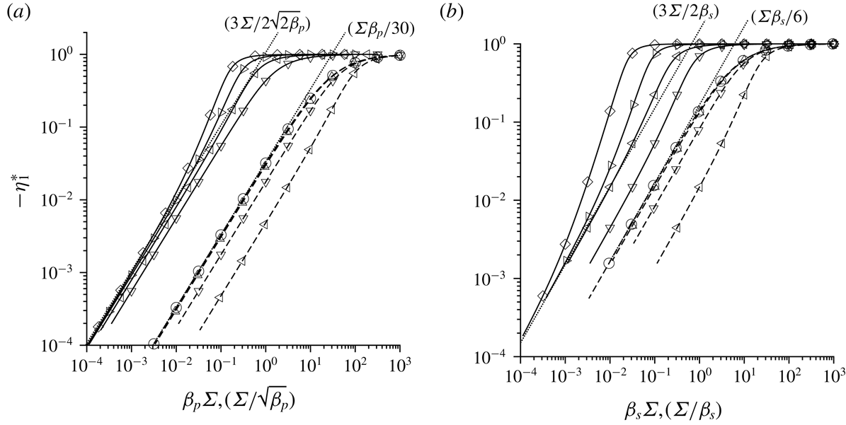
are shown in figure 3 for a uniform particle and figure 4 for a thin shell. In these figures, the asymptotic analysis of §§ 4.1 and 4.2 has been used to rescale the coordinates. The magnitude of the angular velocity
 $\unicode[STIX]{x1D6FA}^{\ast }$
approaches
 $1$
for
 $\unicode[STIX]{x1D6F4}\ll 1$
(4.1), and tends towards
 $\hat{\unicode[STIX]{x1D74E}}\boldsymbol{\cdot }\hat{\boldsymbol{H}}$
for
 $\unicode[STIX]{x1D6F4}\gg 1$
(4.10). A natural definition of the rescaled angular velocity is,
 $$\begin{eqnarray}\displaystyle \unicode[STIX]{x1D6FA}^{\ast \ast }=\frac{\unicode[STIX]{x1D6FA}^{\ast }-\hat{\unicode[STIX]{x1D74E}}\boldsymbol{\cdot }\hat{\boldsymbol{H}}}{1-\hat{\unicode[STIX]{x1D74E}}\boldsymbol{\cdot }\hat{\boldsymbol{H}}}, & & \displaystyle\end{eqnarray}$$
which varies from
 $1$
for
 $\unicode[STIX]{x1D6F4}\ll 1$
to
 $0$
for
 $\unicode[STIX]{x1D6F4}\gg 1$
. The scaled first couple stress coefficient
 $(\unicode[STIX]{x1D702}_{c}^{(1)}/(3\unicode[STIX]{x1D702}\unicode[STIX]{x1D719}/2))$
is
 $0$
for
 $\unicode[STIX]{x1D6F4}=0$
(4.7), and it increases to a maximum value of
 $(1-(\hat{\unicode[STIX]{x1D74E}}\boldsymbol{\cdot }\hat{\boldsymbol{H}})^{2})$
for
 $\unicode[STIX]{x1D6F4}\gg 1$
(4.14). An appropriate definition of the scaled first couple stress coefficient is,
 $$\begin{eqnarray}\displaystyle \unicode[STIX]{x1D702}_{1}^{\ast }=\frac{\unicode[STIX]{x1D702}_{c}^{(1)}}{(3\unicode[STIX]{x1D719}\unicode[STIX]{x1D702}/2)(1-(\hat{\unicode[STIX]{x1D74E}}\boldsymbol{\cdot }\hat{\boldsymbol{H}})^{2})}, & & \displaystyle\end{eqnarray}$$
which varies in the range 0–1. The scaled third couple stress coefficient is proportional to
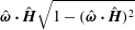 $\hat{\unicode[STIX]{x1D74E}}\boldsymbol{\cdot }\hat{\boldsymbol{H}}\sqrt{1-(\hat{\unicode[STIX]{x1D74E}}\boldsymbol{\cdot }\hat{\boldsymbol{H}})^{2}}$
for
 $\unicode[STIX]{x1D6F4}\ll 1$
(4.8) and for
 $\unicode[STIX]{x1D6F4}\gg 1$
(equation 4.15); a suitable scaled third couple stress coefficient is,
 $$\begin{eqnarray}\displaystyle \unicode[STIX]{x1D702}_{3}^{\ast }=\frac{\unicode[STIX]{x1D702}_{c}^{(3)}}{(3\unicode[STIX]{x1D719}\unicode[STIX]{x1D702}/2)(\hat{\unicode[STIX]{x1D74E}}\boldsymbol{\cdot }\hat{\boldsymbol{H}}\sqrt{1-(\hat{\unicode[STIX]{x1D74E}}\boldsymbol{\cdot }\hat{\boldsymbol{H}})^{2}})}. & & \displaystyle\end{eqnarray}$$
The scaled angular velocity
 $\unicode[STIX]{x1D6FA}^{\ast \ast }$
(a), the scaled first couple stress coefficient
 $\unicode[STIX]{x1D702}_{1}^{\ast }$
(b) and third couple stress coefficient
 $\unicode[STIX]{x1D702}_{3}^{\ast }$
(c), defined in (4.16)–(4.18), as a function of
 $\unicode[STIX]{x1D6F4}$
for a thin shell with
 $\unicode[STIX]{x1D6FD}_{s}=0.3$
(dashed lines),
 $\unicode[STIX]{x1D6FD}_{s}=3$
(solid lines) and
 $\unicode[STIX]{x1D6FD}_{s}=100$
(dotted lines) for ○
 $\hat{\unicode[STIX]{x1D74E}}\boldsymbol{\cdot }\hat{\boldsymbol{H}}=(1/3)$
, ▵
 $\hat{\unicode[STIX]{x1D74E}}\boldsymbol{\cdot }\hat{\boldsymbol{H}}=(1/2)$
, ▿
 $\hat{\unicode[STIX]{x1D74E}}\boldsymbol{\cdot }\hat{\boldsymbol{H}}=(1/\sqrt{2})$
and ♢
 $\hat{\unicode[STIX]{x1D74E}}\boldsymbol{\cdot }\hat{\boldsymbol{H}}=0.99$
.

The magnitude of the angular velocity
 $\unicode[STIX]{x1D6FA}^{\ast \ast }$
(figures 3
a and 4
a) decreases from
 $1$
to
 $\hat{\unicode[STIX]{x1D74E}}\boldsymbol{\cdot }\hat{\boldsymbol{H}}$
over a range of approximately two decades in
 $\unicode[STIX]{x1D6F4}$
. The functional form of
 $\unicode[STIX]{x1D6FA}^{\ast \ast }$
shows a relatively small dependence on
 $\hat{\unicode[STIX]{x1D74E}}\boldsymbol{\cdot }\hat{\boldsymbol{H}}$
for small
 $\unicode[STIX]{x1D6FD}$
, but there is a significant dependence on
 $\hat{\unicode[STIX]{x1D74E}}\boldsymbol{\cdot }\hat{\boldsymbol{H}}$
for
 $\unicode[STIX]{x1D6FD}_{p}=300$
for a uniform particle and
 $\unicode[STIX]{x1D6FD}_{p}=100$
for a thin shell. It is observed that the magnitude of the slope of the
 $\unicode[STIX]{x1D6FA}^{\ast \ast }-\unicode[STIX]{x1D6F4}$
curve increases and appears to diverge at
 $\hat{\unicode[STIX]{x1D74E}}\boldsymbol{\cdot }\hat{\boldsymbol{H}}=(1/3)$
for
 $\unicode[STIX]{x1D6FD}_{p}=300$
for a uniform particle and
 $\unicode[STIX]{x1D6FD}_{s}=100$
for a thin shell. This aspect is analysed in detail in § 6.
In contrast to the angular velocity,
 $\unicode[STIX]{x1D702}_{1}^{\ast }$
and
 $\unicode[STIX]{x1D702}_{3}^{\ast }$
exhibit a remarkable lack of dependence on
 $\hat{\unicode[STIX]{x1D74E}}\boldsymbol{\cdot }\hat{\boldsymbol{H}}$
when
 $\unicode[STIX]{x1D6FD}$
is small; all the results for the first and third couple stress coefficients collapse on to
 $\hat{\unicode[STIX]{x1D74E}}\boldsymbol{\cdot }\hat{\boldsymbol{H}}$
-independent curves over the entire range of
 $\unicode[STIX]{x1D6F4}$
for
 $\unicode[STIX]{x1D6FD}_{p}\leqslant 10$
for a uniform particle and
 $\unicode[STIX]{x1D6FD}_{s}\leqslant 3$
for a thin shell. The scaled first couple stress coefficient
 $\unicode[STIX]{x1D702}_{1}^{\ast }$
increases proportional to
 $\unicode[STIX]{x1D6F4}$
for
 $\unicode[STIX]{x1D6F4}\ll 1$
, and tends to a limiting value of
 $1$
for
 $\unicode[STIX]{x1D6F4}\gg 1$
. For low
 $\unicode[STIX]{x1D6F4}$
and high
 $\unicode[STIX]{x1D6FD}$
, two distinct regions are visible in figures 3(b) and 4(b) for the first couple stress coefficient. These correspond to the two distinct regimes identified in table 1. For a uniform particle,
 $\unicode[STIX]{x1D702}_{1}^{\ast }$
is found to be independent of
 $\unicode[STIX]{x1D6FD}_{p}$
for
 $\unicode[STIX]{x1D6F4}\lesssim 3\times 10^{-2}$
in figure 3(b); this is in agreement with the prediction in the parameter regime
 $\unicode[STIX]{x1D6F4}\ll \unicode[STIX]{x1D6FD}_{p}^{-1/2}$
in table 1. For a thin shell,
 $\unicode[STIX]{x1D702}_{1}^{\ast }$
appears to become independent of
 $\hat{\unicode[STIX]{x1D74E}}\boldsymbol{\cdot }\hat{\boldsymbol{H}}$
only for
 $\unicode[STIX]{x1D6F4}\lesssim 10^{-2}$
; this is due to the more stringent requirement that
 $\unicode[STIX]{x1D6F4}\ll \unicode[STIX]{x1D6FD}_{s}^{-1}$
for a thin shell in table 1. There is an intermediate region,
 $\unicode[STIX]{x1D6F4}\gtrsim 3\times 10^{-2}$
for a uniform particle and
 $\unicode[STIX]{x1D6F4}\gtrsim 10^{-2}$
for a thin shell, where
 $\unicode[STIX]{x1D702}_{1}^{\ast }$
does depend on
 $\hat{\unicode[STIX]{x1D74E}}\boldsymbol{\cdot }\hat{\boldsymbol{H}}$
. In this regime, the variation of
 $\unicode[STIX]{x1D702}_{1}^{\ast }$
with
 $\unicode[STIX]{x1D6F4}$
in agreement with the asymptotic result
 $\unicode[STIX]{x1D702}_{1}^{\ast }\propto \unicode[STIX]{x1D6F4}^{2}$
in table 1. Table 1 also shows that the first couple stress coefficient is proportional to
 $(\hat{\unicode[STIX]{x1D74E}}\boldsymbol{\cdot }\hat{\boldsymbol{H}})^{2}(1-(\hat{\unicode[STIX]{x1D74E}}\boldsymbol{\cdot }\hat{\boldsymbol{H}})^{2})$
in this regime, and therefore the scaled first couple stress coefficient (4.17) does depend on
 $\hat{\unicode[STIX]{x1D74E}}\boldsymbol{\cdot }\hat{\boldsymbol{H}}$
in figures 3(b) and 4(b).
The scaled third couple stress coefficient (figures 3
c and 4
c) increases proportional to
 $\unicode[STIX]{x1D6F4}$
for
 $\unicode[STIX]{x1D6F4}\ll 1$
, and decreases proportional to
 $\unicode[STIX]{x1D6F4}^{-1}$
for
 $\unicode[STIX]{x1D6F4}\gg 1$
. Consistent with the results in table 1, there is only one regime for
 $\unicode[STIX]{x1D6F4}\ll 1$
for the third couple stress coefficient, and
 $\unicode[STIX]{x1D702}_{3}^{\ast }\propto \unicode[STIX]{x1D6F4}$
in this regime. Due to this, there is a remarkable data collapse in the limits
 $\unicode[STIX]{x1D6F4}\ll 1$
and
 $\unicode[STIX]{x1D6F4}\gg 1$
for both low and high
 $\unicode[STIX]{x1D6FD}$
. The appearance of an inflection point close to the maximum in the
 $\unicode[STIX]{x1D702}_{3}^{\ast }$
graph for
 $\hat{\unicode[STIX]{x1D74E}}\boldsymbol{\cdot }\hat{\boldsymbol{H}}=1/3$
is noteworthy; the reason for this is discussed in § 6.
The
 $\unicode[STIX]{x1D6FD}$
dependence of the couple stress coefficients is examined in further detail for
 $\hat{\unicode[STIX]{x1D74E}}\boldsymbol{\cdot }\hat{\boldsymbol{H}}=(1/\sqrt{2})$
in figures 5 and 6. For a uniform particle, the asymptotic expression for
 $\unicode[STIX]{x1D702}_{1}^{\ast }$
in table 1 is proportional to
 $\unicode[STIX]{x1D6FD}_{p}\unicode[STIX]{x1D6F4}$
for
 $\unicode[STIX]{x1D6FD}_{p}\ll 1$
, and proportional to
 $(\unicode[STIX]{x1D6F4}/\sqrt{\unicode[STIX]{x1D6FD}_{p}})$
for
 $\unicode[STIX]{x1D6FD}_{p}\gg 1$
and
 $\unicode[STIX]{x1D6F4}\ll \unicode[STIX]{x1D6FD}_{p}^{-1/2}$
. In figure 5, the dashed lines show the first couple stress plotted against
 $(\unicode[STIX]{x1D6FD}_{p}\unicode[STIX]{x1D6F4})$
, and the dotted lines show the asymptotic expression for
 $\unicode[STIX]{x1D6FD}_{p}\ll 1$
. It is observed that the asymptotic expression provides an excellent fit for the
 $(\unicode[STIX]{x1D6FD}_{p}\unicode[STIX]{x1D6F4})\lesssim 1$
and
 $\unicode[STIX]{x1D6FD}_{p}\leqslant 3$
. There is some deviation from the asymptotic expression for
 $\unicode[STIX]{x1D6FD}_{p}\geqslant 10$
. The solid lines in figure 5 are graphs of
 $\unicode[STIX]{x1D702}_{1}^{\ast }$
versus
 $(\unicode[STIX]{x1D6F4}/\sqrt{\unicode[STIX]{x1D6FD}_{p}})$
. These provide good fits for the first couple stress coefficient for
 $(\unicode[STIX]{x1D6F4}/\sqrt{\unicode[STIX]{x1D6FD}_{p}})\leqslant 10^{-3}$
and
 $\unicode[STIX]{x1D6FD}_{p}\geqslant 30$
. There is an intermediate range of
 $3<\unicode[STIX]{x1D6FD}_{p}<30$
where the asymptotic expressions are not in quantitative agreement with the numerical results. In addition, there is a range of
 $10^{-3}\leqslant \unicode[STIX]{x1D6F4}\leqslant 10^{-1}$
, corresponding to the limit
 $\unicode[STIX]{x1D6FD}_{p}\gg 1$
and
 $1\gg \unicode[STIX]{x1D6F4}\gg \unicode[STIX]{x1D6FD}_{p}^{-1/2}$
in table 1, where the there is a dependence on
 $\unicode[STIX]{x1D6FD}_{p}$
. In this range, we find that a graph of
 $\unicode[STIX]{x1D702}_{1}^{\ast }$
versus
 $\unicode[STIX]{x1D6F4}$
results in data collapse for
 $\unicode[STIX]{x1D6FD}_{p}\geqslant 30$
; this result is not shown here for conciseness. For a thin shell, the qualitative behaviour of
 $\unicode[STIX]{x1D702}_{1}^{\ast }$
is similar for a uniform particle. The asymptotic expression for
 $\unicode[STIX]{x1D702}_{1}^{\ast }$
in table 1 is proportional to
 $\unicode[STIX]{x1D6FD}_{s}\unicode[STIX]{x1D6F4}$
for
 $\unicode[STIX]{x1D6FD}_{s}\ll 1$
. This is in agreement with the numerical result in figure 5(b) for
 $\unicode[STIX]{x1D6FD}_{s}\leqslant 1$
and
 $\unicode[STIX]{x1D6F4}\leqslant 1$
. For
 $\unicode[STIX]{x1D6FD}_{s}\gg 1$
and
 $\unicode[STIX]{x1D6F4}\ll \unicode[STIX]{x1D6FD}_{s}^{-1}$
,
 $\unicode[STIX]{x1D702}_{1}^{\ast }$
is proportional to
 $(\unicode[STIX]{x1D6F4}/\unicode[STIX]{x1D6FD}_{s})$
in table 1. The numerical result in figure 5 is in agreement with the asymptotic expression for
 $\unicode[STIX]{x1D6FD}_{s}\geqslant 10$
in the limit
 $\unicode[STIX]{x1D6F4}\ll 1$
. However, the asymptotic expression is applicable for a smaller range in
 $\unicode[STIX]{x1D6F4}$
in comparison to that for a uniform particle, due to the stronger condition
 $\unicode[STIX]{x1D6F4}\ll \unicode[STIX]{x1D6FD}_{s}^{-1}$
. In the intermediate regime
 $\unicode[STIX]{x1D6FD}_{s}^{-1}\ll \unicode[STIX]{x1D6F4}\ll 1$
, there is collapse of the data when
 $\unicode[STIX]{x1D702}_{1}^{\ast }$
is plotted as a function of
 $\unicode[STIX]{x1D6F4}$
; this regime is not shown here for conciseness.
The negative of the scaled first couple stress coefficient
 $-\unicode[STIX]{x1D702}_{1}^{\ast }$
for
 $\hat{\unicode[STIX]{x1D74E}}\boldsymbol{\cdot }\hat{\boldsymbol{H}}=(1/\sqrt{2})$
for a uniform particle (a) as a function of
 $\unicode[STIX]{x1D6FD}_{p}\unicode[STIX]{x1D6F4}$
(dashed lines) and
 $(\unicode[STIX]{x1D6F4}/\sqrt{\unicode[STIX]{x1D6FD}_{p}})$
(solid lines) for
 $\unicode[STIX]{x1D6FD}_{p}=1$
(○),
 $\unicode[STIX]{x1D6FD}_{p}=3$
(▵),
 $\unicode[STIX]{x1D6FD}_{p}=10$
(▿),
 $\unicode[STIX]{x1D6FD}_{p}=30$
(◃),
 $\unicode[STIX]{x1D6FD}_{p}=100$
(▹) and
 $\unicode[STIX]{x1D6FD}_{p}=300$
(♢); and a thin shell (b) as a function of
 $(\unicode[STIX]{x1D6FD}_{s}\unicode[STIX]{x1D6F4})$
(dashed lines) and
 $(\unicode[STIX]{x1D6F4}/\unicode[STIX]{x1D6FD}_{s})$
(solid lines) for
 $\unicode[STIX]{x1D6FD}_{s}=0.3$
(○),
 $\unicode[STIX]{x1D6FD}_{s}=1$
(▵),
 $\unicode[STIX]{x1D6FD}_{s}=3$
(▿),
 $\unicode[STIX]{x1D6FD}_{s}=10$
(◃),
 $\unicode[STIX]{x1D6FD}_{s}=30$
(▹) and
 $\unicode[STIX]{x1D6FD}_{s}=100$
(♢).

The third couple stress coefficient is shown as a function of
 $\unicode[STIX]{x1D6F4}$
in figure 6. In table 1, the third couple stress coefficient is proportional to
 $\unicode[STIX]{x1D6FD}^{2}\unicode[STIX]{x1D6F4}$
for
 $\unicode[STIX]{x1D6F4}\ll 1$
and
 $\unicode[STIX]{x1D6FD}\ll 1$
. Figure 6 shows that this relationship is valid for a uniform particle for
 $\unicode[STIX]{x1D6FD}_{p}\leqslant 3$
and
 $\unicode[STIX]{x1D6F4}\lesssim 1$
, and for a thin shell for
 $\unicode[STIX]{x1D6FD}_{s}\leqslant 1$
and
 $\unicode[STIX]{x1D6F4}\lesssim 1$
. In table 1, the third couple stress coefficient proportional to
 $\unicode[STIX]{x1D6F4}$
for
 $\unicode[STIX]{x1D6F4}\ll 1$
and
 $\unicode[STIX]{x1D6FD}\gg 1$
. Figure 6 indicates that this relationship is valid for
 $\unicode[STIX]{x1D6FD}_{p}\geqslant 30$
and
 $\unicode[STIX]{x1D6F4}\lesssim 1$
for a uniform particle, and for
 $\unicode[STIX]{x1D6FD}_{s}\geqslant 10$
and
 $\unicode[STIX]{x1D6F4}\lesssim 1$
for a thin shell. There is an intermediate interval of a decade,
 $3\lesssim \unicode[STIX]{x1D6FD}_{p}\lesssim 30$
for a uniform particle and
 $1\lesssim \unicode[STIX]{x1D6FD}_{s}\lesssim 10$
for a thin shell, where the asymptotic expressions are not quantitatively accurate. In the limit
 $\unicode[STIX]{x1D6F4}\gg 1$
, the asymptotic expressions for
 $\unicode[STIX]{x1D6FD}\ll 1$
and
 $\unicode[STIX]{x1D6FD}\gg 1$
in table 2 numerically close for a uniform particle. Figure 6(a) shows the numerical results are in agreement with the predicted
 $\unicode[STIX]{x1D6F4}^{-1}$
behaviour, and it is even possible to discern the small numerical difference in the coefficients for the limits
 $\unicode[STIX]{x1D6FD}_{p}\ll 1$
and
 $\unicode[STIX]{x1D6FD}_{p}\gg 1$
for a uniform particle. For a thin shell, the asymptotic expressions for
 $\unicode[STIX]{x1D6F4}\gg 1$
are identical in the limits
 $\unicode[STIX]{x1D6FD}_{s}\ll 1$
and
 $\unicode[STIX]{x1D6FD}_{s}\gg 1$
, and these are in quantitative agreement with the numerical results. For high
 $\unicode[STIX]{x1D6FD}$
, there is a transition between the low and high
 $\unicode[STIX]{x1D6F4}$
regimes at
 $\unicode[STIX]{x1D6F4}\approx 3$
for a uniform particle and
 $\unicode[STIX]{x1D6F4}\approx 2$
for a thin shell. For low
 $\unicode[STIX]{x1D6FD}$
, there is a transition from low to high
 $\unicode[STIX]{x1D6F4}$
regime at
 $\unicode[STIX]{x1D6F4}\approx 15\unicode[STIX]{x1D6FD}_{p}^{-1}$
for a uniform particle, and
 $\unicode[STIX]{x1D6F4}\approx 15\unicode[STIX]{x1D6FD}_{s}^{-1}$
for a thin shell.
The scaled third couple stress coefficient
 $\unicode[STIX]{x1D702}_{3}^{\ast }$
for
 $\hat{\unicode[STIX]{x1D74E}}\boldsymbol{\cdot }\hat{\boldsymbol{H}}=(1/\sqrt{2})$
as a function of
 $\unicode[STIX]{x1D6F4}$
for a uniform particle (a) for
 $\unicode[STIX]{x1D6FD}_{p}=1$
(○),
 $\unicode[STIX]{x1D6FD}_{p}=3$
(▵),
 $\unicode[STIX]{x1D6FD}_{p}=10$
(▿),
 $\unicode[STIX]{x1D6FD}_{p}=30$
(◃),
 $\unicode[STIX]{x1D6FD}_{p}=100$
(▹) and
 $\unicode[STIX]{x1D6FD}_{p}=300$
(♢), and a thin shell (b) for
 $\unicode[STIX]{x1D6FD}_{s}=0.3$
(○),
 $\unicode[STIX]{x1D6FD}_{s}=1$
(▵),
 $\unicode[STIX]{x1D6FD}_{s}=3$
(▿),
 $\unicode[STIX]{x1D6FD}_{s}=10$
(◃),
 $\unicode[STIX]{x1D6FD}_{s}=30$
(▹) and
 $\unicode[STIX]{x1D6FD}_{s}=100$
(♢). In (a) the dashed lines, from right to left, are the relations
 $\unicode[STIX]{x1D702}_{3}^{\ast }=(\unicode[STIX]{x1D6F4}\unicode[STIX]{x1D6FD}_{p}^{2}/315)$
(see table 1) for
 $\unicode[STIX]{x1D6FD}_{p}=1$
,
 $3$
and
 $10$
respectively. In (b) the dashed lines, from right to left, are the relations
 $\unicode[STIX]{x1D702}_{3}^{\ast }=(\unicode[STIX]{x1D6F4}\unicode[STIX]{x1D6FD}_{s}^{2}/18)$
(see table 1) for
 $\unicode[STIX]{x1D6FD}_{s}=0.3$
,
 $1$
and
 $3$
respectively.

5 Perpendicular magnetic field
A special case arises when the direction of the magnetic field is perpendicular to the direction of the fluid vorticity at the particle centre. In this case, the particle angular velocity vector is parallel to the fluid vorticity, and perpendicular to the magnetic field. Equations (2.6) and (2.7) are trivially satisfied if
 $\hat{\unicode[STIX]{x1D6FA}}_{\boldsymbol{H}}=0$
and
 $\hat{\unicode[STIX]{x1D6FA}}_{\unicode[STIX]{x1D74E}}=1$
, and it is necessary to solve (2.5) to determine the particle angular velocity. The asymptotic expression in § 4.1 is applicable for a perpendicular magnetic field, but the asymptotic result in § 4.2 is not applicable, because the terms in the expansion in (4.10)–(4.15) were calculated assuming that
 $\hat{\unicode[STIX]{x1D74E}}\boldsymbol{\cdot }\hat{\boldsymbol{H}}$
is finite and
 $\unicode[STIX]{x1D6F4}\gg 1$
.
For a perpendicular magnetic field, equation (2.5) reduces to,
 $$\begin{eqnarray}\displaystyle 1-\unicode[STIX]{x1D6FA}^{\ast }-\unicode[STIX]{x1D6F4}\,M_{I}(\unicode[STIX]{x1D6FD}\unicode[STIX]{x1D6FA}^{\ast })=0. & & \displaystyle\end{eqnarray}$$
The second and third couple stress coefficients are zero for a perpendicular magnetic field, and the first couple stress coefficient is given by (3.5) with
 $\hat{\unicode[STIX]{x1D6FA}}_{\unicode[STIX]{x1D74E}}=1$
.
5.1 Uniform particle
The left side of (5.1) is shown as a function of
 $\unicode[STIX]{x1D6F4}$
for
 $\unicode[STIX]{x1D6FD}_{p}=200$
in figure 7. When
 $\unicode[STIX]{x1D6F4}$
is increased from 5 to 6, there is first a transition from one solution to three solutions. As
 $\unicode[STIX]{x1D6F4}$
is further increased from 6 to 7, there is a second transition from three real solutions to one real solutions. Thus, there is an finite range of
 $\unicode[STIX]{x1D6F4}$
for which there are three solutions for a fixed value of
 $\unicode[STIX]{x1D6FD}_{p}$
; there is only one solution outside this range.
The left side of (5.1) shown as a function of
 $\unicode[STIX]{x1D6FA}^{\ast }$
for
 $\unicode[STIX]{x1D6FD}_{p}=200$
and
 $\unicode[STIX]{x1D6F4}=5$
(○),
 $6$
(▵) and
 $7$
(▿).

The solution
 $\unicode[STIX]{x1D6FA}^{\ast }$
of (5.1) for a uniform particle (a) and the negative of the scaled first couple stress coefficient
 $-\unicode[STIX]{x1D702}_{1}^{\ast }$
(b) as a function of
 $\unicode[STIX]{x1D6F4}$
for
 $\unicode[STIX]{x1D6FD}_{p}=50$
(○), 100 (▵), 200 (▿), 400 (♢) and 800 (▫). The dotted lines at the right in (a) show the limiting value
 $30(\unicode[STIX]{x1D6F4}\unicode[STIX]{x1D6FD}_{p})^{-1}$
for
 $\unicode[STIX]{x1D6F4}\gg 1$
(5.3), and the dotted lines on the left in (b) show the limiting value
 $\unicode[STIX]{x1D6F4}M_{I}(\unicode[STIX]{x1D6FD}_{p})$
.

The solutions
 $\unicode[STIX]{x1D6FA}^{\ast }$
for (5.1) are shown as a function of
 $\unicode[STIX]{x1D6F4}$
for different values of
 $\unicode[STIX]{x1D6FD}_{p}$
in figure 8(a), and the corresponding scaled first couple stress coefficient (equation (4.17)) is shown in figure 8(b). It is evident that (5.1) has a unique solution,
 $$\begin{eqnarray}\displaystyle \left.\begin{array}{@{}c@{}}\displaystyle \unicode[STIX]{x1D6FA}^{\ast }=1-\unicode[STIX]{x1D6F4}M_{I}(\unicode[STIX]{x1D6FD}_{p}),\\ \displaystyle \unicode[STIX]{x1D702}_{1}^{\ast }=-\unicode[STIX]{x1D6F4}M_{I}(\unicode[STIX]{x1D6FD}_{p}),\end{array}\right\} & & \displaystyle\end{eqnarray}$$
for
 $\unicode[STIX]{x1D6F4}\ll 1$
. The asymptotic results for
 $\unicode[STIX]{x1D702}_{1}^{\ast }$
for
 $\unicode[STIX]{x1D6F4}\ll 1$
, shown by the dotted lines on the left in figure 8(b), are in good agreement with the numerical results. For
 $\unicode[STIX]{x1D6F4}\unicode[STIX]{x1D6FD}_{p}\gg 1$
, the solution
 $\unicode[STIX]{x1D6FA}^{\ast }$
decreases proportional to
 $(\unicode[STIX]{x1D6F4}\unicode[STIX]{x1D6FD}_{p})^{-1}$
, as shown by the dotted lines on the right in figure 8(a). This solution is inferred from (5.1), if we take the limit
 $\unicode[STIX]{x1D6FA}^{\ast }\ll 1$
,
 $M_{I}(\unicode[STIX]{x1D6FD}_{p}\unicode[STIX]{x1D6FA}^{\ast })=(\unicode[STIX]{x1D6FD}_{p}\unicode[STIX]{x1D6FA}^{\ast }/30)$
for
 $\unicode[STIX]{x1D6FD}_{p}\unicode[STIX]{x1D6FA}^{\ast }\ll 1$
(2.12), and
 $\unicode[STIX]{x1D6FA}^{\ast }\unicode[STIX]{x1D6F4}\unicode[STIX]{x1D6FD}_{p}\sim 1$
,
 $$\begin{eqnarray}\displaystyle \unicode[STIX]{x1D6FA}^{\ast }=\frac{30}{30+\unicode[STIX]{x1D6F4}\unicode[STIX]{x1D6FD}_{p}}. & & \displaystyle\end{eqnarray}$$
For
 $\unicode[STIX]{x1D6F4}\unicode[STIX]{x1D6FD}_{p}\gg 30$
, the solution (5.3) is approximately
 $30(\unicode[STIX]{x1D6F4}\unicode[STIX]{x1D6FD}_{p})^{-1}$
, shown by the dashed lines on the right in figure 8(a). Thus, asymptotic analysis can be used to determine the values of
 $\unicode[STIX]{x1D6FA}^{\ast }$
and
 $\unicode[STIX]{x1D702}_{1}^{\ast }$
for
 $\unicode[STIX]{x1D6F4}\ll 1$
and
 $\unicode[STIX]{x1D6F4}\gg 1$
.
For
 $\unicode[STIX]{x1D6FD}_{p}=50$
, figure 8(a) shows that the solution for
 $\unicode[STIX]{x1D6FA}^{\ast }$
monotonically decreases as
 $\unicode[STIX]{x1D6F4}$
increases. When
 $\unicode[STIX]{x1D6FD}_{p}$
is greater than
 $100$
, there is a range of values of
 $\unicode[STIX]{x1D6F4}$
for which there are three solutions for
 $\unicode[STIX]{x1D6FA}^{\ast }$
. There are two turning points of infinite slope where the solution turns back on itself. There is a stable solution for
 $\unicode[STIX]{x1D6FA}^{\ast }$
which is a continuation of the solution for
 $\unicode[STIX]{x1D6F4}\ll 1$
(5.2), and another stable solution which is a continuation of the solution for
 $\unicode[STIX]{x1D6F4}\gg 1$
, both shown by the solid lines. In between, there is a solution shown by the dashed line, which is an unstable solution.
A salient feature of the turning points in figure 8(a) are the values of
 $\unicode[STIX]{x1D6F4}$
and
 $\unicode[STIX]{x1D6FA}^{\ast }$
at right and left turning points. The value of
 $\unicode[STIX]{x1D6F4}$
at the right turning point shows a significant increase as
 $\unicode[STIX]{x1D6FD}_{p}$
is increased, whereas the value of
 $\unicode[STIX]{x1D6FA}^{\ast }$
is approximately the same. At the left turning point, the value of
 $\unicode[STIX]{x1D6F4}$
is approximately independent of
 $\unicode[STIX]{x1D6FD}_{p}$
, while the value of
 $\unicode[STIX]{x1D6FA}^{\ast }$
decreases significantly as
 $\unicode[STIX]{x1D6FD}_{p}$
is increased. The value of
 $\unicode[STIX]{x1D6F4}$
at the right and left turning points are shown in figure 9(a), while the values of
 $\unicode[STIX]{x1D6FA}^{\ast }$
are shown in figure 9(b). For
 $\unicode[STIX]{x1D6FD}_{p}<93.02$
, there is only one solution for
 $\unicode[STIX]{x1D6FA}^{\ast }$
for all values of
 $\unicode[STIX]{x1D6F4}$
. For
 $\unicode[STIX]{x1D6FD}_{p}>93.02$
, there are three real solutions when
 $\unicode[STIX]{x1D6F4}$
has a value in between a minimum, which tends to a constant value of 5.63 for
 $\unicode[STIX]{x1D6FD}_{p}\gg 1$
, and a maximum which tends to
 $(4\sqrt{2\unicode[STIX]{x1D6FD}_{p}}/9\sqrt{3})$
for
 $\unicode[STIX]{x1D6FD}_{p}\gg 1$
.
For a uniform particle, as a function of
 $\unicode[STIX]{x1D6FD}_{p}$
, the lower limit (○) and upper limit (▵) of the range of
 $\unicode[STIX]{x1D6F4}$
for the existence of multiple steady states (a), and the angular velocity
 $\unicode[STIX]{x1D6FA}^{\ast }$
(b) on the upper and lower branches for the values of
 $\unicode[STIX]{x1D6F4}$
shown in (a). The dashed line in (a) is
 $(\unicode[STIX]{x1D6F4}/\sqrt{\unicode[STIX]{x1D6FD}_{p}})=(4\sqrt{2}/9\sqrt{3})$
. The value
 $\unicode[STIX]{x1D6FA}^{\ast }=(1/3)$
at the boundary
 $(\unicode[STIX]{x1D6F4}/\sqrt{\unicode[STIX]{x1D6FD}_{p}})=(4\sqrt{2}/9\sqrt{3})$
is shown by the dashed line in (b). The dotted line in (a) shows
 $\unicode[STIX]{x1D6F4}=5.63$
, and in (b) shows the asymptote
 $\unicode[STIX]{x1D6FA}^{\ast }=(11.61/\unicode[STIX]{x1D6FD}_{p})$
.

In appendix B, the
 $\unicode[STIX]{x1D6F4}$
and
 $\unicode[STIX]{x1D6FD}$
dependence of the right and left turning points in figure 9(a), and the reason for the multistability, are examined using asymptotic analysis in the limit
 $\unicode[STIX]{x1D6FD}_{p}\unicode[STIX]{x1D6FA}^{\ast }\gg 1$
.
5.2 Thin shell
The results for the scaled angular velocity of a thin shell are briefly presented, since these are very similar to those for a uniform particle. The torque balance equation at steady state is,
 $$\begin{eqnarray}\displaystyle 1-\unicode[STIX]{x1D6FA}^{\ast }-\frac{3\unicode[STIX]{x1D6F4}\unicode[STIX]{x1D6FD}_{s}\unicode[STIX]{x1D6FA}^{\ast }}{2(9+\unicode[STIX]{x1D6FD}_{s}^{2}\unicode[STIX]{x1D6FA}^{\ast ^{2}})}=0. & & \displaystyle\end{eqnarray}$$
The solutions for the angular velocity are shown as a function of
 $\unicode[STIX]{x1D6F4}$
for different values of
 $\unicode[STIX]{x1D6FD}_{s}$
in figure 10(a), and the scaled first couple stress coefficient in (b). The transition between a unique solution and multiple solutions takes place at a value of
 $\unicode[STIX]{x1D6FD}_{s}$
that is about 15.7, which is approximately 6 times smaller than the value of
 $\unicode[STIX]{x1D6FD}_{p}$
at which the transition takes place for a uniform particle. For
 $(\unicode[STIX]{x1D6FD}_{s}\unicode[STIX]{x1D6FA}^{\ast })\ll 1$
and
 $\unicode[STIX]{x1D6FA}^{\ast }\sim 1$
, there is a unique solution for (5.4),
 $$\begin{eqnarray}\displaystyle \unicode[STIX]{x1D6FA}^{\ast }=\frac{1}{1+(\unicode[STIX]{x1D6F4}\unicode[STIX]{x1D6FD}_{s}/6)}. & & \displaystyle\end{eqnarray}$$
This solution predicts the decrease in
 $\unicode[STIX]{x1D6FA}^{\ast }$
from
 $1$
for small
 $\unicode[STIX]{x1D6F4}$
. In the limit
 $(\unicode[STIX]{x1D6FD}_{s}\unicode[STIX]{x1D6FA}^{\ast })\ll 1$
and
 $\unicode[STIX]{x1D6F4}\gg 1$
, the unique solution for
 $\unicode[STIX]{x1D6FA}^{\ast }$
is similar to the solution (5.3) for a uniform particle,
 $$\begin{eqnarray}\displaystyle \unicode[STIX]{x1D6FA}^{\ast }=6(\unicode[STIX]{x1D6F4}\unicode[STIX]{x1D6FD}_{s})^{-1}. & & \displaystyle\end{eqnarray}$$
This solution is shown by the dotted lines on the right side of figure 10(a).
The solution
 $\unicode[STIX]{x1D6FA}^{\ast }$
of (5.4) for a thin shell (a) and the negative of the scaled first couple stress coefficient
 $-\unicode[STIX]{x1D702}_{1}^{\ast }$
(b) as a function of
 $\unicode[STIX]{x1D6F4}$
for
 $\unicode[STIX]{x1D6FD}_{s}=10$
(○), 20 (▵), 40 (▿), 80 (♢) and 160 (▫). The dotted lines on the right in (a) show the limiting value
 $6(\unicode[STIX]{x1D6F4}\unicode[STIX]{x1D6FD}_{s})^{-1}$
(5.6). The dotted lines on the left in (b) show the limiting value
 $\unicode[STIX]{x1D6F4}M_{I}(\unicode[STIX]{x1D6FD}_{s})$
.

The values of
 $\unicode[STIX]{x1D6F4}$
and
 $\unicode[STIX]{x1D6FA}^{\ast }$
at the left and right turning points in figure 10(a) are shown in figure 11(a,b). At the right turning point,
 $\unicode[STIX]{x1D6F4}$
tends to
 $(\unicode[STIX]{x1D6FD}_{s}/6)$
and
 $\unicode[STIX]{x1D6FA}^{\ast }$
tends to
 $0.5$
for
 $\unicode[STIX]{x1D6FD}_{s}\gg 1$
. These are examined using asymptotic analysis in appendix B.
For a thin shell, as a function of
 $\unicode[STIX]{x1D6FD}_{s}$
, the lower limit (○) and upper limit (▵) of the range of
 $\unicode[STIX]{x1D6F4}$
for which multiple steady states exists for the particle angular velocity (a), and the angular velocity
 $\unicode[STIX]{x1D6FA}^{\ast }$
(b) on the upper and lower branches for the
 $\unicode[STIX]{x1D6F4}$
shown in (a). The asymptotic expression
 $(\unicode[STIX]{x1D6F4}=\unicode[STIX]{x1D6FD}_{s}/6)$
(B 3) is the region below the dashed line in (a). The value
 $\unicode[STIX]{x1D6FA}^{\ast }=(1/2)$
for
 $\unicode[STIX]{x1D6FD}_{s}\gg 1$
and
 $\unicode[STIX]{x1D6F4}=(\unicode[STIX]{x1D6FD}_{s}/6)$
is shown by the dashed line in (b). The dotted line in (a) shows
 $\unicode[STIX]{x1D6F4}=4$
, and in (b) shows
 $\unicode[STIX]{x1D6FA}^{\ast }=(3/\unicode[STIX]{x1D6FD}_{s})$
.
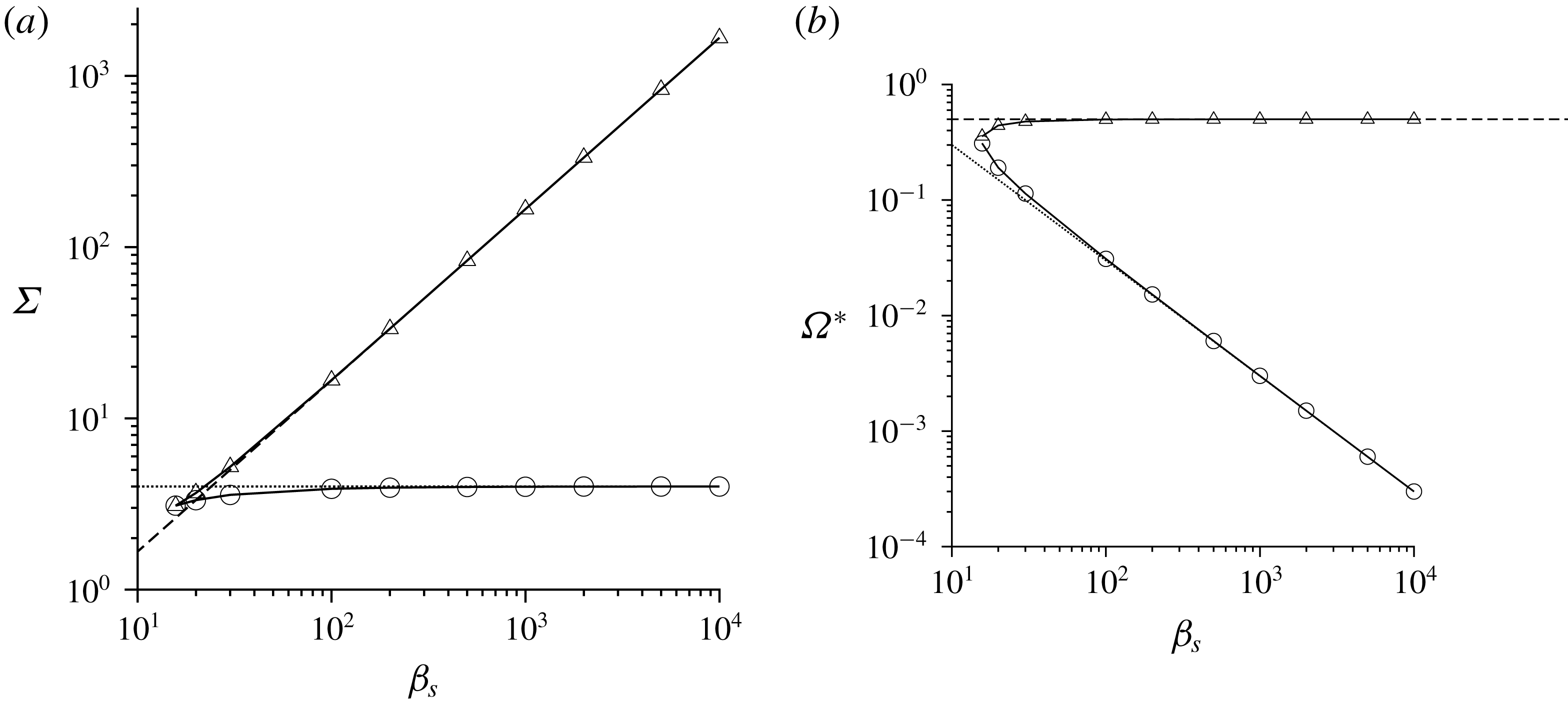
6 Near-perpendicular magnetic field
In § 4, a unique solution was obtained for the angular velocity and the couple stress coefficients for fixed
 $\unicode[STIX]{x1D6F4}$
and
 $\unicode[STIX]{x1D6FD}$
, whereas in § 5, there was the possibility of multiple steady states for a perpendicular magnetic field for sufficiently large
 $\unicode[STIX]{x1D6FD}$
. In this section, we consider a near-perpendicular magnetic field,
 $\hat{\unicode[STIX]{x1D74E}}\boldsymbol{\cdot }\hat{\boldsymbol{H}}\ll 1$
, in order to examine the range of
 $\hat{\unicode[STIX]{x1D74E}}\boldsymbol{\cdot }\hat{\boldsymbol{H}}$
for which there is the possibility of multiple steady states.
The numerical solutions show that there are multiple steady states even when
 $\hat{\unicode[STIX]{x1D74E}}\boldsymbol{\cdot }\hat{\boldsymbol{H}}$
is small but not zero. These multiple steady states are shown for
 $\hat{\unicode[STIX]{x1D74E}}\boldsymbol{\cdot }\hat{\boldsymbol{H}}=0.1$
in figure 12 for a uniform particle and figure 13 for a thin shell. Similar to a perpendicular magnetic field, multiple steady states are observed for high values of
 $\unicode[STIX]{x1D6FD}$
, that is,
 $\unicode[STIX]{x1D6FD}_{p}>100$
for a uniform particle and
 $\unicode[STIX]{x1D6FD}_{p}>10$
for a thin shell. However, the variation of the scaled angular velocity and the first couple stress coefficient with
 $\unicode[STIX]{x1D6F4}$
are qualitatively different from those for a perpendicular magnetic field in figures 8 and 10. The scaled angular velocity
 $\unicode[STIX]{x1D6FA}^{\ast \ast }$
decreases proportional to
 $\unicode[STIX]{x1D6F4}^{-2}$
for
 $\unicode[STIX]{x1D6F4}\gg 1$
and
 $\hat{\unicode[STIX]{x1D74E}}\boldsymbol{\cdot }\hat{\boldsymbol{H}}=0.1$
in figures 12(a) and 13(a), in contrast to the decrease proportional to
 $\unicode[STIX]{x1D6F4}^{-1}$
for a perpendicular magnetic field. The multiple steady states at
 $\hat{\unicode[STIX]{x1D74E}}\boldsymbol{\cdot }\hat{\boldsymbol{H}}=0.1$
are a continuation of the point of infinite slope at
 $\hat{\unicode[STIX]{x1D74E}}\boldsymbol{\cdot }\hat{\boldsymbol{H}}=(1/3)$
for an oblique magnetic field in figures 3(a) and 4(a); this was briefly pointed out in § 4. The scaled first couple stress coefficient tends to the asymptotic value for
 $\unicode[STIX]{x1D6F4}\ll 1$
for an oblique magnetic field in table 1, instead of the value
 $-\unicode[STIX]{x1D6F4}M_{I}(\unicode[STIX]{x1D6FD})$
for a perpendicular magnetic field in figures 8(b) and 10(b). In addition, the scaled third couple stress coefficient (figures 12
c and 13
c) is found to converge to the limits in table 1 for
 $\unicode[STIX]{x1D6F4}\ll 1$
, and table 2 for
 $\unicode[STIX]{x1D6F4}\gg 1$
. However, multiple steady states for the third couple stress coefficient are clearly visible, and the right turning point is close to the maximum. This feature appears to be a continuation of the cusp in the scaled third couple stress coefficient at
 $\hat{\unicode[STIX]{x1D74E}}\boldsymbol{\cdot }\hat{\boldsymbol{H}}=(1/3)$
in figures 3(c) and 4(c), as briefly highlighted in § 4.
The scaled angular velocity
 $\unicode[STIX]{x1D6FA}^{\ast \ast }$
(4.16) as a function of
 $\unicode[STIX]{x1D6F4}$
(a), the negative of the scaled first couple stress coefficient
 $-\unicode[STIX]{x1D702}_{1}^{\ast }$
(4.17) as a function of
 $(\unicode[STIX]{x1D6F4}/\sqrt{\unicode[STIX]{x1D6FD}_{p}})$
(b) and the scaled third couple stress coefficient
 $\unicode[STIX]{x1D702}_{3}^{\ast }$
(4.18) as a function of
 $\unicode[STIX]{x1D6F4}$
(c) for a uniform particle for
 $\hat{\unicode[STIX]{x1D74E}}\boldsymbol{\cdot }\hat{\boldsymbol{H}}=0.1$
and
 $\unicode[STIX]{x1D6FD}_{p}=100$
(○),
 $300$
(▵),
 $1000$
(▿),
 $3000$
(◃) and
 $10\,000$
(▹).

The scaled angular velocity
 $\unicode[STIX]{x1D6FA}^{\ast \ast }$
(4.16) as a function of
 $\unicode[STIX]{x1D6F4}$
(a), the negative of the scaled first couple stress coefficient
 $-\unicode[STIX]{x1D702}_{1}^{\ast }$
(4.17) as a function of
 $(\unicode[STIX]{x1D6F4}/\unicode[STIX]{x1D6FD}_{s})$
(b) and the scaled third couple stress coefficient
 $\unicode[STIX]{x1D702}_{3}^{\ast }$
(4.18) as a function of
 $\unicode[STIX]{x1D6F4}$
(c) for a thin shell for
 $\hat{\unicode[STIX]{x1D74E}}\boldsymbol{\cdot }\hat{\boldsymbol{H}}=0.1$
and
 $\unicode[STIX]{x1D6FD}_{p}=10$
(○),
 $30$
(▵),
 $100$
(▿),
 $300$
(◃).

The reason for the multiple steady states is examined using asymptotic analysis in appendix C. The predictions of the asymptotic analysis for the existence of three real solutions for
 $\hat{\unicode[STIX]{x1D6FA}}_{\boldsymbol{H}}$
are compared with the numerical solutions for a uniform particle in figure 14, and for a thin shell in figure 15. Multiple solutions are found for a uniform particle for
 $\unicode[STIX]{x1D6FD}_{p}>100$
, and for a thin shell for
 $\unicode[STIX]{x1D6FD}_{s}>30$
. For a uniform particle, the asymptotic results in (C 4) and (C 5) are in agreement with numerical results only for a very high value of
 $\unicode[STIX]{x1D6FD}_{p}=10^{4}$
. For a thin shell, the asymptotic results are in reasonable agreement even for a much lower value of
 $\unicode[STIX]{x1D6FD}_{s}=300$
. In both cases, the results diverge from the numerical result as
 $\hat{\unicode[STIX]{x1D74E}}\boldsymbol{\cdot }\hat{\boldsymbol{H}}$
decreases. This is due to a violation of the requirement that
 $\hat{\unicode[STIX]{x1D74E}}\boldsymbol{\cdot }\hat{\boldsymbol{H}}\gg \unicode[STIX]{x1D6FD}_{p}^{-1/2}$
for a uniform particle and
 $\hat{\unicode[STIX]{x1D74E}}\boldsymbol{\cdot }\hat{\boldsymbol{H}}\gg \unicode[STIX]{x1D6FD}_{s}^{-1}$
for the asymptotic results (C 4) and (C 5) to be valid.
For a uniform particle, as a function of
 $\hat{\unicode[STIX]{x1D74E}}\boldsymbol{\cdot }\hat{\boldsymbol{H}}$
, the lower and upper bounds of
 $\unicode[STIX]{x1D6F4}$
for the existence of three steady states (a), the value of
 $\unicode[STIX]{x1D6FA}^{\ast }$
at the upper and lower bounds (b) for ○
 $\unicode[STIX]{x1D6FD}_{p}=100$
, ▵
 $\unicode[STIX]{x1D6FD}_{p}=300$
, ▿
 $\unicode[STIX]{x1D6FD}_{p}=1000$
, ♢
 $\unicode[STIX]{x1D6FD}_{p}=10\,000$
. The solid lines show the asymptotic result (C 4) and (C 5).

For a thin shell, as a function of
 $\hat{\unicode[STIX]{x1D74E}}\boldsymbol{\cdot }\hat{\boldsymbol{H}}$
, the lower and upper bounds of
 $\unicode[STIX]{x1D6F4}$
for the existence of three steady states (a), the value of
 $\unicode[STIX]{x1D6FA}^{\ast }$
at the lower and upper bounds (b) for ○
 $\unicode[STIX]{x1D6FD}_{p}=30$
, ▵
 $\unicode[STIX]{x1D6FD}_{s}=100$
, ▿
 $\unicode[STIX]{x1D6FD}_{s}=300$
, ♢
 $\unicode[STIX]{x1D6FD}_{s}=1000$
. The solid lines show the asymptotic result (C 4) and (C 5).

7 Conclusions
7.1 Parameter regimes
The couple stress coefficients depend on two parameters, the ratio of the magnetic and viscous torques
 $\unicode[STIX]{x1D6F4}=(\unicode[STIX]{x1D707}_{0}H_{0}^{2}/4\unicode[STIX]{x03C0}\unicode[STIX]{x1D702}|\unicode[STIX]{x1D74E}|)$
, and the product of the vorticity and the current relaxation time
 $\unicode[STIX]{x1D6FD}_{p}=(|\unicode[STIX]{x1D74E}|\unicode[STIX]{x1D707}_{0}R^{2}/2\unicode[STIX]{x1D71A})$
for a uniform particle or
 $\unicode[STIX]{x1D6FD}_{s}=(|\unicode[STIX]{x1D74E}|\unicode[STIX]{x1D707}_{0}R^{2}\unicode[STIX]{x1D6FF}/2\unicode[STIX]{x1D71A})$
for a thin shell. The dimensionless parameter
 $\unicode[STIX]{x1D6F4}$
is independent of the particle radius, and is only a function of the magnetic field, the fluid vorticity and the viscosity. The parameter
 $\unicode[STIX]{x1D6FD}$
does depend on the particle radius and the electrical resistivity of the particle, but is independent of the applied magnetic field. Thus, a change in the magnetic field results in a change in
 $\unicode[STIX]{x1D6F4}$
but not
 $\unicode[STIX]{x1D6FD}$
, whereas a change in the particle radius alters
 $\unicode[STIX]{x1D6FD}$
but not
 $\unicode[STIX]{x1D6F4}$
. The magnetic permeability of free space is
 $\unicode[STIX]{x1D707}_{0}=4\unicode[STIX]{x03C0}\times 10^{-7}~\text{kg m s}^{-2}~\text{A}^{-2}$
, while a typical value of the resistivity
 $\unicode[STIX]{x1D71A}$
for metals is
 $1.5\times 10^{-8}~\text{kg}~\text{m}^{3}~\text{s}^{-3}~\text{A}^{-2}$
. For these values, the parameter
 $\unicode[STIX]{x1D6FD}_{p}\approx 40R^{2}|\unicode[STIX]{x1D74E}|$
for a uniform particle and
 $\unicode[STIX]{x1D6FD}_{s}\approx 40R^{2}\unicode[STIX]{x1D6FF}|\unicode[STIX]{x1D74E}|$
for a thin shell, where
 $R$
and
 $|\unicode[STIX]{x1D74E}|$
are expressed in m and s
 $^{-1}$
respectively. Therefore, the parameter
 $\unicode[STIX]{x1D6FD}$
is
 $O(1)$
only for very high strain rates of the order of
 $10^{3}{-}10^{4}~\text{s}^{-1}$
even for millimetre-sized metal particles in a viscous liquid. However, there are now reports of ultra-low resistivity in composites of graphene/carbon nanotubes with metals, which have resistivity up to two orders of magnitude smaller than metals (Hjortstam et al.
Reference Hjortstam, Isberg, Söderholm and Dai2004; Zheng et al.
Reference Zheng, Zheng, Huo, Wu, Shao, Zheng, Zheng, Qui, Liu and Zhang2018). This might render it feasible to access the high
 $\unicode[STIX]{x1D6FD}$
regime with particles in the range
 $0.1{-}1$
mm, and observe the multiple steady states that are predicted here. The results in the high
 $\unicode[STIX]{x1D6FD}$
regime could also be applicable for superconducting particles, where the resistivity decreases to zero because the magnetic flux lines are expelled from the particle. Type I superconductors are not suitable for this purpose, because the resistivity decreases to zero discontinuously. The induced magnetic moment for a type I superconductor is directly proportional to the angular velocity (Holdeman Reference Holdeman1975), and so there is no possibility of multiple steady states. There is a continuous decrease in the resistivity in type II superconductors, and so they could be possible to access the high
 $\unicode[STIX]{x1D6FD}$
regime. In fact, the equations for type II superconductors are only a small modification of the equations used in appendix A (Schafer & Heiden Reference Schafer and Heiden1978), in that the permeability is a function of the magnetic field, and Ohm’s law has to be modified to include a critical current density and a flux flow conductivity. Type II superconductors also have relatively high critical temperatures, enabling easier experimentation. The adaptation of the present analysis for superconducting particles is the subject of future work.
The parameter
 $\unicode[STIX]{x1D6F4}$
can be varied over a relatively wide range in real applications. The Earth’s magnetic flux density
 $\unicode[STIX]{x1D707}_{0}H_{0}$
is less than 65 microteslas, which is
 $6.5\times 10^{-5}~\text{kg}~\text{s}^{-2}~\text{A}^{-1}$
, but a magnetic flux density of
 $1~\text{kg}~\text{s}^{-2}~\text{A}^{-1}$
is easily achievable in practice. Therefore, the magnetic field strength
 $H_{0}$
can be varied in the range
 $50{-}10^{6}~\text{A}~\text{m}^{-1}$
. The characteristic magnetic torque
 $\unicode[STIX]{x1D707}_{0}H_{0}^{2}$
can, therefore, be varied in the range
 $3\times 10^{-3}{-}10^{6}~\text{kg}~\text{m}~\text{s}^{-2}$
. Hydrodynamic torques lower or higher than the characteristic magnetic torque are easily generated by using low/high viscosity fluids and by varying the strain rate. Therefore, the entire range
 $\unicode[STIX]{x1D6F4}\ll 1$
and
 $\unicode[STIX]{x1D6F4}\gg 1$
is easily accessible in practical applications.
An issue of interest is the expected enhancement in the shear viscosity due to the eddy current torque. It is important to note that the couple stress coefficients are proportional to the antisymmetric part of the rate of deformation tensor, in contrast to the viscous stress, which is proportional to the symmetric part. It bears reiterating that the effect of the eddy current torques results in antisymmetric stresses which act in the planes perpendicular to the flow plane, and these are likely to give rise to complicated and interesting phenomena which cannot be considered a simple enhancement of the shear viscosity. The effect of couple stresses can be modelled as a modified viscosity only for simple flows. For a unidirectional flow with velocity in the
 $x$
direction, velocity gradient in the
 $y$
direction and vorticity in the
 $z$
direction, it is easily shown that the enhancement to the viscosity is the negative of the first couple stress coefficient,
 $-\unicode[STIX]{x1D702}_{c}^{(1)}$
.
7.2 Geometries
The calculations have been carried out for two geometries, a uniform particle and a thin shell with thickness small compared to the radius, in order to examine the generality of the results. The major difference between the two is the scaling of the imaginary part of the magnetic moment,
 $M_{I}$
, in the limit of high
 $\unicode[STIX]{x1D6FD}$
, between the equations (2.13) for a uniform particle and (2.15) for a thin shell. Due to this, there is a difference in the first couple stress coefficient in the limit of small
 $\unicode[STIX]{x1D6F4}$
and high
 $\unicode[STIX]{x1D6FD}$
in the regime
 $\unicode[STIX]{x1D6F4}\gg \unicode[STIX]{x1D6FD}_{p}^{-1/2}$
for a uniform particle and
 $\unicode[STIX]{x1D6F4}\gg \unicode[STIX]{x1D6FD}_{s}^{-1}$
for a thin shell, as shown in table 1. The real part of the magnetic moment
 $M_{R}$
tends to
 $-(1/2)$
for both uniform particles and thin shells. Since the real part affects the third couple stress coefficient, there is no difference in the scaling of the third couple stress coefficient between uniform particles and thin shells. There is also no difference in the dominant terms for the first and third couple stress coefficients for high
 $\unicode[STIX]{x1D6F4}$
. The calculations for a shell of finite thickness can also be carried out using the results in appendix A if necessary; apart from the difference at low
 $\unicode[STIX]{x1D6F4}$
and high
 $\unicode[STIX]{x1D6FD}$
, the scaling relations derived in § 4 are robust for different shell thicknesses, though the coefficients in the scaling relations do depend on the ratio of the shell thickness and radius.
7.3 Couple stress coefficients
A suspension of conducting particles in a magnetic field is a micro-polar fluid, in which the antisymmetric part of the stress tensor has components perpendicular to all three coordinate planes in general. Here, a specific orthonormal coordinate system has been chosen, where one axis
 $\hat{\unicode[STIX]{x1D74E}}$
is along the vorticity direction, the second
 $(\hat{\boldsymbol{H}}-\hat{\unicode[STIX]{x1D74E}}(\hat{\unicode[STIX]{x1D74E}}\boldsymbol{\cdot }\hat{\boldsymbol{H}}))/\sqrt{1-(\hat{\unicode[STIX]{x1D74E}}\boldsymbol{\cdot }\hat{\boldsymbol{H}})^{2}}$
is perpendicular to the
 $\hat{\unicode[STIX]{x1D74E}}$
in the
 $\hat{\unicode[STIX]{x1D74E}}{-}\hat{\boldsymbol{H}}$
plane, and the third
 $(\hat{\unicode[STIX]{x1D74E}}\boldsymbol{\times }\hat{\boldsymbol{H}})/\sqrt{1-(\hat{\unicode[STIX]{x1D74E}}\boldsymbol{\cdot }\hat{\boldsymbol{H}})^{2}}$
is perpendicular to the
 $\hat{\unicode[STIX]{x1D74E}}{-}\hat{\boldsymbol{H}}$
plane. The rheology is simplified due to the relation (3.10), which arises because there is no torque parallel to the magnetic field; due to this, there are only two independent couple stress coefficients. An alternate choice is to consider
 $\hat{\boldsymbol{H}}$
as one axis. In this case, the couple stress coefficient in the plane perpendicular to
 $\hat{\boldsymbol{H}}$
would have been zero. Here, we have preferred to align one axis along the vorticity direction, since this direction is usually of importance for the fluid dynamics.
An unusual characteristic of the rheology is the presence of an antisymmetric component of the stress tensor, proportional to the third couple stress coefficient
 $\unicode[STIX]{x1D702}_{c}^{(3)}$
, in the
 $\hat{\unicode[STIX]{x1D74E}}{-}\hat{\boldsymbol{H}}$
plane, when
 $\hat{\unicode[STIX]{x1D74E}}$
and
 $\hat{\boldsymbol{H}}$
are not orthogonal. This is due to the ‘precession torque’ in the direction perpendicular to the
 $\hat{\unicode[STIX]{x1D74E}}{-}\hat{\boldsymbol{H}}$
plane when a conductor rotates in a magnetic field. Due to this, there could be an antisymmetric stress in a conducting fluid even perpendicular to the flow plane, that is, the plane containing the velocity and the velocity gradient, for two-dimensional flows. The effect of such a stress on the stability of two-dimensional flows and the generation of secondary flows could reveal novel phenomena which are worth exploring.
Asymptotic analysis has been used to calculate the couple stress coefficients in the limits
 $\unicode[STIX]{x1D6F4}\ll 1$
and
 $\unicode[STIX]{x1D6F4}\gg 1$
as a function of the parameter
 $\unicode[STIX]{x1D6FD}$
. For
 $\unicode[STIX]{x1D6F4}\ll 1$
, a regular perturbation expansion can be used in the parameter
 $\unicode[STIX]{x1D6F4}$
. In the leading approximation, the torque due to the magnetic field is neglected, and the particle angular velocity is equal to one half of the fluid vorticity. The
 $O(\unicode[STIX]{x1D6F4})$
correction to the particle angular velocity and the couple stress coefficients are calculated in (4.1), (4.7) and (4.8), and are listed for uniform particles and thin shells in table 1. For
 $\unicode[STIX]{x1D6FD}\ll 1$
, the first couple stress coefficient is independent of
 $|\unicode[STIX]{x1D74E}|$
and the third couple stress coefficient is proportional to
 $|\unicode[STIX]{x1D74E}|$
in all cases. For
 $\unicode[STIX]{x1D6FD}\gg 1$
,
 $\unicode[STIX]{x1D702}_{c}^{(1)}$
and
 $\unicode[STIX]{x1D702}_{c}^{(3)}$
exhibit unusual inverse power-law dependences on
 $|\unicode[STIX]{x1D74E}|$
because
 $\unicode[STIX]{x1D6FD}_{p}$
and
 $\unicode[STIX]{x1D6FD}_{s}$
are proportional to
 $|\unicode[STIX]{x1D74E}|$
,
 $\unicode[STIX]{x1D6F4}$
is inversely proportional to
 $|\unicode[STIX]{x1D74E}|$
and the first couple stress coefficient, in particular, has an inverse power-law dependence on
 $\unicode[STIX]{x1D6FD}_{p}$
and
 $\unicode[STIX]{x1D6FD}_{s}$
.
In the limit
 $\unicode[STIX]{x1D6F4}\gg 1$
, one would simplistically expect the particles to stop rotating because the retarding magnetic torque is much larger than the hydrodynamic torque. However, in the absence of particle rotation, there is no eddy current and therefore no magnetic torque. The solution to this paradox is that the particle rotation axis aligns close to the magnetic field, so that the
 $(1-\hat{\unicode[STIX]{x1D6FA}}_{\boldsymbol{H}}^{2})\sim \unicode[STIX]{x1D6F4}^{-1}$
in (2.5)–(2.7), and a balance is achieved between the hydrodynamic and magnetic torques. The asymptotic results in (4.10), (4.14) and (4.15) indicate that the first couple stress coefficient tends to a constant value
 $(3\unicode[STIX]{x1D719}\unicode[STIX]{x1D702}/2)(1-(\hat{\unicode[STIX]{x1D74E}}\boldsymbol{\cdot }\hat{\boldsymbol{H}})^{2})$
in this limit, and the third couple stress coefficients decreases proportional to
 $\unicode[STIX]{x1D6F4}^{-1}$
. When expressed in terms of the vorticity and dimensional parameters, table 2 indicates that the first couple stress coefficient is independent of
 $|\unicode[STIX]{x1D74E}|$
and the third couple stress coefficient is proportional to
 $|\unicode[STIX]{x1D74E}|$
. Both of these dependences are robust because they are independent of the parameter
 $\unicode[STIX]{x1D6FD}$
and of the configuration (uniform particle or thin shell), and therefore this parameter regime is suitable for the design of fluids with well-defined non-Newtonian rheological properties.
The couple stress coefficients can be further simplified for small
 $\unicode[STIX]{x1D6FD}$
, which is of most relevance to practical applications. An important simplification was made by defining the scaled angular velocity (4.16) and the scaled couple stress coefficients (equations (4.17)–(4.18)). Figures 3–4 show that the couple stress coefficients are independent of
 $\hat{\unicode[STIX]{x1D74E}}\boldsymbol{\cdot }\hat{\boldsymbol{H}}$
for small values of
 $\unicode[STIX]{x1D6FD}$
, indicating that universal forms for the scaled couple stress coefficients can be used for any relative orientation between the vorticity and the magnetic field. A further simplification is shown in figure 5, where
 $\unicode[STIX]{x1D702}_{1}^{\ast }$
is only a function of one parameter,
 $(\unicode[STIX]{x1D6FD}_{p}\unicode[STIX]{x1D6F4})$
for
 $\unicode[STIX]{x1D6FD}_{p}\leqslant 10$
for a uniform particle, and a function of
 $(\unicode[STIX]{x1D6FD}_{s}\unicode[STIX]{x1D6F4})$
alone for
 $\unicode[STIX]{x1D6FD}_{s}\leqslant 3$
for a thin shell. Similarly, figure 6 shows that the
 $\unicode[STIX]{x1D702}_{3}^{\ast }$
increases proportional to
 $\unicode[STIX]{x1D6F4}\unicode[STIX]{x1D6FD}_{p}^{2}$
and
 $\unicode[STIX]{x1D6F4}\unicode[STIX]{x1D6FD}_{s}^{2}$
for small
 $\unicode[STIX]{x1D6F4}$
, and decreases proportional to
 $\unicode[STIX]{x1D6F4}^{-1}$
independent of
 $\unicode[STIX]{x1D6FD}$
for
 $\unicode[STIX]{x1D6F4}\gg 1$
. Therefore, simple relations can be used for the first and third couple stress coefficients for small
 $\unicode[STIX]{x1D6FD}$
.
The situation in the limit
 $\unicode[STIX]{x1D6FD}\gg 1$
is different for the two couple stress coefficients. The third couple stress coefficient
 $\unicode[STIX]{x1D702}_{3}^{\ast }$
has a very simple variation proportional to
 $\unicode[STIX]{x1D6F4}$
for
 $\unicode[STIX]{x1D6F4}\ll 1$
and proportional to
 $\unicode[STIX]{x1D6F4}^{-1}$
for
 $\unicode[STIX]{x1D6F4}\gg 1$
. This is because
 $\unicode[STIX]{x1D702}_{3}^{\ast }$
depends on the real part of the induced magnetic moment
 $M_{R}$
in (2.8) and (2.14), and
 $M_{R}$
tends to a constant value of
 $-(1/2)$
independent of
 $\unicode[STIX]{x1D6FD}$
and the configuration (uniform particle or thin shell) for
 $\unicode[STIX]{x1D6FD}\gg 1$
. The form of
 $\unicode[STIX]{x1D702}_{1}^{\ast }$
for large
 $\unicode[STIX]{x1D6FD}$
is more complicated, because it depends on the imaginary part of the induced magnetic moment
 $M_{I}$
in (2.9) and (2.15), and this has different power-law dependences on
 $\unicode[STIX]{x1D6FD}_{p}$
for a uniform particle (2.13) and on
 $\unicode[STIX]{x1D6FD}_{s}$
for a thin shell (equation (2.15)). For
 $\unicode[STIX]{x1D6F4}\ll 1$
, scaling laws are obtained in two different regimes. For
 $\unicode[STIX]{x1D6F4}\ll \unicode[STIX]{x1D6FD}_{p}^{-1/2}$
for a uniform particle and
 $\unicode[STIX]{x1D6F4}\ll \unicode[STIX]{x1D6FD}_{s}^{-1}$
for a thin shell,
 $\unicode[STIX]{x1D702}_{1}^{\ast }$
is independent of
 $\hat{\unicode[STIX]{x1D74E}}\boldsymbol{\cdot }\hat{\boldsymbol{H}}$
and it depends only on one parameter,
 $(\unicode[STIX]{x1D6F4}/\unicode[STIX]{x1D6FD}_{p}^{1/2})$
for a uniform particle and
 $(\unicode[STIX]{x1D6F4}/\unicode[STIX]{x1D6FD}_{s})$
for a thin shell. The coefficient
 $\unicode[STIX]{x1D702}_{1}^{\ast }$
does depend on
 $\hat{\unicode[STIX]{x1D74E}}\boldsymbol{\cdot }\hat{\boldsymbol{H}}$
for
 $\unicode[STIX]{x1D6FD}_{p}^{-1/2}\ll \unicode[STIX]{x1D6F4}\ll 1$
for a uniform particle and
 $\unicode[STIX]{x1D6FD}_{s}^{-1}\ll \unicode[STIX]{x1D6F4}\ll 1$
for a thin shell.
An issue of interest is the expected enhancement in the shear viscosity due to the eddy current torque. It bears reiterating that the effect of the eddy current torques results in antisymmetric stresses which act in the planes perpendicular to the flow plane, and these are likely to give rise to complicated and interesting phenomena which cannot be considered a simple enhancement of the shear viscosity. The effect of couple stresses can be modelled as a modified viscosity only for simple flows. For a unidirectional flow with velocity in the
 $x$
direction, velocity gradient in the
 $y$
direction and vorticity in the
 $z$
direction, it is easily shown that the enhancement to the viscosity is the negative of the first couple stress coefficient,
 $-\unicode[STIX]{x1D702}_{c}^{(1)}$
.
Since a single-particle calculation is carried out in the dilute limit, the couple stress coefficients are proportional to the volume fraction
 $\unicode[STIX]{x1D719}$
. This is similar to the Einstein viscosity for a particle suspension. The scaled couple stress coefficient has been defined as
 $\unicode[STIX]{x1D702}_{1}^{\ast }=(\unicode[STIX]{x1D702}_{c}^{(1)}/((3\unicode[STIX]{x1D719}/2)\unicode[STIX]{x1D702}(1-(\hat{\unicode[STIX]{x1D74E}}\boldsymbol{\cdot }\hat{\boldsymbol{H}})^{2})))$
, where
 $\unicode[STIX]{x1D702}$
is the fluid viscosity. The scaled couple stress coefficient
 $\unicode[STIX]{x1D702}_{1}^{\ast }$
has a maximum value of
 $1$
in the limit
 $H\gg 1$
for all values of
 $\unicode[STIX]{x1D6FD}$
, and therefore, the viscosity enhancement is
 $(3\unicode[STIX]{x1D719}\unicode[STIX]{x1D702}(1-(\hat{\unicode[STIX]{x1D74E}}\boldsymbol{\cdot }\hat{\boldsymbol{H}})^{2})/2)$
. For a perpendicular magnetic field, the viscosity enhancement is
 $(3\unicode[STIX]{x1D719}\unicode[STIX]{x1D702}/2)$
, which is comparable to the enhancement of the viscosity in a particle suspension proportional to
 $(5\unicode[STIX]{x1D719}\unicode[STIX]{x1D702}/2)$
due to the symmetric force moment in an extensional flow.
7.4 Perpendicular and near-perpendicular magnetic fields
Multiple steady states are observed when the vorticity and the magnetic field are perpendicular or almost perpendicular, for high
 $\unicode[STIX]{x1D6FD}$
. For a perpendicular magnetic field, the particle angular velocity is parallel to the vorticity, and the second and third couple stress coefficients are zero. It is necessary to solve one torque balance equation, equation (5.1), to determine the angular velocity and first couple stress coefficient. The underlying reason for the multiple steady states is that the relation between the imaginary part of the magnetic moment
 $M_{I}$
and the angular velocity is nonlinear in the limit of high
 $\unicode[STIX]{x1D6FD}$
, as shown in (2.13) and (2.15), resulting in a nonlinear relationship between the torque and the angular velocity. It should be noted that for a perpendicular magnetic field, the torque depends only on
 $M_{I}$
. Multiple solutions are observed for
 $\unicode[STIX]{x1D6FD}_{p}>93$
for a uniform particle and
 $\unicode[STIX]{x1D6FD}_{s}>15.7$
for a thin shell. The right and left turning points in the graphs of the angular velocity and first couple stress difference versus
 $\unicode[STIX]{x1D6F4}$
have been determined using asymptotic analysis in appendix B, where the high
 $\unicode[STIX]{x1D6FD}$
approximations, equations (2.13) and (2.15) are used for the eddy current torques. These are in good quantitative agreement with numerical results for high
 $\unicode[STIX]{x1D6FD}$
.
Multiple steady states can exist for a near-perpendicular magnetic field, where
 $\hat{\unicode[STIX]{x1D74E}}\boldsymbol{\cdot }\hat{\boldsymbol{H}}$
is less than
 $1/3$
, in the limit of large
 $\unicode[STIX]{x1D6FD}$
. The reason for multiple steady states in this case is qualitatively different from that for a perpendicular magnetic field. For high
 $\unicode[STIX]{x1D6FD}$
, the imaginary part of the magnetic moment
 $M_{I}$
decreases to zero (equations (2.13) and (2.15)), whereas the real part
 $M_{R}$
tends to a constant value
 $-(1/2)$
(equations (2.11) and (2.14)). In the limit of high
 $\unicode[STIX]{x1D6FD}$
, the term proportional to
 $M_{I}$
is neglected in (2.17), and
 $M_{R}$
is set equal to
 $-(1/2)$
in (2.18), to obtain equations that are independent of
 $\unicode[STIX]{x1D6FD}$
or the configuration (uniform particle or thin shell). Using this approximation, it is shown that there could be multiple steady states only for
 $\hat{\unicode[STIX]{x1D74E}}\boldsymbol{\cdot }\hat{\boldsymbol{H}}<(1/3)$
, and the values of
 $\unicode[STIX]{x1D6F4}$
at the two turning points have been calculated using asymptotic analysis in appendix C. The numerical results are in agreement with the asymptotic solutions only for very large values of
 $\unicode[STIX]{x1D6FD}$
, that is,
 $\unicode[STIX]{x1D6FD}_{p}=10^{4}$
for a uniform particle and
 $\unicode[STIX]{x1D6FD}_{s}=10^{3}$
for a thin shell. However, there is a small interval of
 $\unicode[STIX]{x1D6F4}$
where there are multiple solutions even for
 $\unicode[STIX]{x1D6FD}_{p}=100$
for a uniform particle and
 $\unicode[STIX]{x1D6FD}_{s}=30$
for a thin shell.
The transition between the solutions for the perpendicular and near-perpendicular magnetic field occurs when the magnitude of the term on the right in (2.18) becomes larger than the term on the right in (2.17), that is, for
 $|\hat{\unicode[STIX]{x1D74E}}\boldsymbol{\cdot }\hat{\boldsymbol{H}}M_{R}(\unicode[STIX]{x1D6FD}\unicode[STIX]{x1D6FA}^{\ast })|>|M_{I}(\unicode[STIX]{x1D6FD}\unicode[STIX]{x1D6FA}^{\ast })|$
. Since
 $M_{R}$
tends to
 $-(1/2)$
for
 $\unicode[STIX]{x1D6FD}\unicode[STIX]{x1D6FA}^{\ast }\gg 1$
, this implies that
 $\hat{\unicode[STIX]{x1D74E}}\boldsymbol{\cdot }\hat{\boldsymbol{H}}\gg \unicode[STIX]{x1D6FD}_{p}^{-1/2}$
for a uniform particle, and
 $\hat{\unicode[STIX]{x1D74E}}\boldsymbol{\cdot }\hat{\boldsymbol{H}}\gg \unicode[STIX]{x1D6FD}_{s}^{-1}$
for a thin shell.
The existence of multiple steady states suggests the intriguing possibility of ‘spin banding’ in these suspensions, where different particle angular velocities could co-exist for the same fluid vorticity and magnetic field; this is an exciting prospect that does not seem to have been proposed before. The evolution and rheology of spin-banded states necessarily depends on nature of particle interactions at the two-particle level and beyond, and this is an area that merits further study.
7.5 Particle interactions and migration
Some aspects of the hydrodynamic interactions between particles and the flow in finite channels were considered in appendix D. One important result is the convergence of the integrals in unbounded systems for the flow generated by particles that exert a net torque on the fluid. This is surprising, because the velocity disturbance due to the particle decreases proportional to
 $(1/r^{2})$
, while the vorticity disturbance decreases proportional to
 $(1/r^{3})$
. The velocity disturbance is expected to be zero in a uniform suspension of rotating particles due to symmetry. However, the net vorticity disturbance also turns out to be finite, because the integral over the solid angle of the vorticity disturbance in (D 2) for
 $|\boldsymbol{x}-\boldsymbol{x}^{\prime }|>R$
turns out to be zero. Due to this, the integral for the mean vorticity is convergent. The integrals for the mean square velocity and vorticity are also convergent, and these have been calculated in § D.1.
Particle migration is predicted in a finite channel due to gradients in the particle angular velocity or the volume fraction in §§ D.2 and D.3. A gradient in the particle angular velocity could result from the gradient in the vorticity even in a uniform magnetic field. When the gradient is in the cross-stream direction for a unidirectional flow in a channel, and the particle angular velocity is in the direction of the fluid vorticity, the secondary velocity is opposite to the flow direction. However, if there is a component of the angular velocity in the flow–gradient plane due to a precession torque, there is a secondary flow velocity generated in the spanwise direction as well. Thus, an oblique magnetic field, coupled with a volume fraction or vorticity gradient in the cross-stream direction, could cause particle migration in the spanwise direction. The secondary flow could be useful for separation of conducting particles under an applied magnetic field, and the drift velocity generated is proportional to
 $\unicode[STIX]{x1D719}\bar{u}$
where
 $\bar{u}$
is the average velocity,
 $\unicode[STIX]{x1D719}$
is the volume fraction and the length scale for the vorticity and volume fraction gradient is considered to be the channel height
 $h$
. There is also a drift velocity due to a gradient in the fluid vorticity, but this drift is only in the streamwise direction if the vorticity is perpendicular to the flow plane. This drift velocity is proportional to
 $(\bar{u}R^{2}/h^{2})$
.
Acknowledgements
The author would like to thank the Department of Science and Technology, Government and the J. R. D. Tata Memorial Trust for financial support. The author would like to thank Mr C. G. Subramaniam for useful discussions.
Appendix A. Torque due to eddy currents
A conducting spherical shell of inner radius
 $R_{i}$
, outer radius
 $R$
, electrical resistivity
 $\unicode[STIX]{x1D71A}$
and permeability
 $\unicode[STIX]{x1D707}_{0}$
is rotating with angular velocity
 $\unicode[STIX]{x1D734}$
in an insulating fluid. The relative permeability
 $\unicode[STIX]{x1D707}$
of the particle and fluid are considered to be
 $1$
, because the calculation is restricted to non-ferromagnetic materials. The particle is subject to a constant external magnetic field
 $\boldsymbol{H}_{0}$
far from the particle. A spherical coordinate system is used where
 $r$
is the distance from the centre of the shell. The Maxwell equations for the magnetic field
 $\boldsymbol{H}$
and electric field
 $\boldsymbol{E}$
are,
 $$\begin{eqnarray}\displaystyle \unicode[STIX]{x1D735}\boldsymbol{\times }\boldsymbol{H} & = & \displaystyle 0\quad \text{for }r<R_{i}\quad \text{and}\quad r>R,\nonumber\\ \displaystyle & = & \displaystyle \boldsymbol{J}\quad \text{for }R_{i}<r<R,\end{eqnarray}$$
 $$\begin{eqnarray}\displaystyle \unicode[STIX]{x1D735}\boldsymbol{\times }\boldsymbol{E}=-\unicode[STIX]{x1D707}_{0}\frac{\text{d}\boldsymbol{H}}{\text{d}t}\quad \text{for }R_{i}<r<R, & & \displaystyle\end{eqnarray}$$
and the current in the conducting particle is related to the electric field by Ohm’s law,
 $$\begin{eqnarray}\displaystyle \boldsymbol{J}=\frac{\boldsymbol{E}}{\unicode[STIX]{x1D71A}}. & & \displaystyle\end{eqnarray}$$
The magnetic field is written as the curl of the solenoidal magnetic potential
 $\boldsymbol{A}$
,
 $$\begin{eqnarray}\boldsymbol{H}=\unicode[STIX]{x1D735}\boldsymbol{\times }\boldsymbol{A}.\end{eqnarray}$$
Equation (A 2) can be used to express the induced electric field as,
 $$\begin{eqnarray}\displaystyle \boldsymbol{E}=-\unicode[STIX]{x1D707}_{0}\frac{\text{d}\boldsymbol{A}}{\text{d}t}. & & \displaystyle\end{eqnarray}$$
Combining (A 1), (A 3), (A 4) and (A 5), we obtain an equation for the vector potential,
 $$\begin{eqnarray}-\frac{\unicode[STIX]{x1D707}_{0}}{\unicode[STIX]{x1D71A}}\frac{\text{d}\boldsymbol{A}}{\text{d}t}+\unicode[STIX]{x1D6FB}^{2}\boldsymbol{A}=0\quad \text{for }R_{i}<r<R,\end{eqnarray}$$
within the spherical shell. Since the material inside and outside is insulating, the equation for the magnetic potential is,
 $$\begin{eqnarray}\unicode[STIX]{x1D6FB}^{2}\boldsymbol{A}=0\quad \text{for }r<R_{i}\quad \text{and}\quad r>R.\end{eqnarray}$$
The two coupled equations have to be solved with boundary conditions
 $\boldsymbol{H}=\boldsymbol{H}_{0}$
far
 $\boldsymbol{H}$
is finite at
 $r=0$
, and the matching condition that the magnetic field is continuous across the surface.
The solution is obtained in a coordinate system with the axis of rotation along the
 $z$
direction and the applied magnetic field is in the
 $x{-}z$
plane, with components
 $H_{0x}$
and
 $H_{0z}$
in the
 $x$
and
 $z$
directions far from the particle. Since the particle is rotating in the magnetic field, it is necessary to express the magnetic field in a coordinate system
 $\boldsymbol{x}^{\prime }$
rotating with the particle. The fixed and rotating coordinates are related by the rotation matrix,
 $$\begin{eqnarray}\boldsymbol{x}^{\prime }=\unicode[STIX]{x1D64D}\boldsymbol{\cdot }\boldsymbol{x},\end{eqnarray}$$
where
 $\unicode[STIX]{x1D64D}$
is the rotation matrix. Since the angular velocity is aligned with the
 $z$
axis, the rotation matrix is,
 $$\begin{eqnarray}\displaystyle \unicode[STIX]{x1D64D} & = & \displaystyle \left(\begin{array}{@{}ccc@{}}\cos (\unicode[STIX]{x1D6FA}t) & \sin (\unicode[STIX]{x1D6FA}t) & 0\\ -\sin (\unicode[STIX]{x1D6FA}t) & \cos (\unicode[STIX]{x1D6FA}t) & 0\\ 0 & 0 & 1\end{array}\right)\nonumber\\ \displaystyle & = & \displaystyle \text{Re}\left(\begin{array}{@{}ccc@{}}\exp (-\imath \unicode[STIX]{x1D6FA}t) & \imath \exp (-\imath \unicode[STIX]{x1D6FA}t) & 0\\ -\imath \exp (-\imath \unicode[STIX]{x1D6FA}t) & \exp (-\imath \unicode[STIX]{x1D6FA}t) & 0\\ 0 & 0 & 1\end{array}\right),\end{eqnarray}$$
where
 $\unicode[STIX]{x1D6FA}$
is the magnitude of the angular velocity
 $\unicode[STIX]{x1D734}$
In the rotating frame, the components of the applied magnetic field are,
 $$\begin{eqnarray}\displaystyle \left.\begin{array}{@{}c@{}}\displaystyle H_{0x^{\prime }}^{\prime }=\text{Re}(\exp (-\imath \unicode[STIX]{x1D6FA}t)H_{0x}),\\ \displaystyle H_{0y^{\prime }}^{\prime }=\text{Re}(-\imath \exp (-\imath \unicode[STIX]{x1D6FA}t)H_{0x}),\\ H_{0z^{\prime }}^{\prime }=H_{0z}.\end{array}\right\} & & \displaystyle\end{eqnarray}$$
In the following analysis, the superscript
 $^{\prime }$
is used for quantities referenced to the rotating coordinate system.
Within the shell, the divergence of
 $\boldsymbol{A}^{\prime }$
is zero, and the vector
 $\boldsymbol{A}$
is a linear function of the applied field
 $\boldsymbol{H}_{0}^{\prime }$
. Therefore, the solution for (A 6) in the conductor for
 $R_{i}<r<R$
is of the form,
 $$\begin{eqnarray}\displaystyle \boldsymbol{A}^{\prime }=\unicode[STIX]{x1D735}\boldsymbol{\times }(A_{s}(r)\boldsymbol{H}_{0}^{\prime }), & & \displaystyle\end{eqnarray}$$
where the scalar function
 $A_{s}(r)$
is a solution of the equation
 $$\begin{eqnarray}\displaystyle \unicode[STIX]{x1D6FB}^{2}A_{s}(r)+k^{2}A_{s}(r)=0, & & \displaystyle\end{eqnarray}$$
where
 $k=\sqrt{\imath \unicode[STIX]{x1D6FA}\unicode[STIX]{x1D707}_{0}/\unicode[STIX]{x1D71A}}$
.
The solution of (A 12) for the scalar field
 $A_{s}(r)$
is
 $$\begin{eqnarray}\displaystyle A_{s}(r)=\frac{A_{s1}\sin (kr)}{r}+\frac{A_{s2}\cos (kr)}{r}, & & \displaystyle\end{eqnarray}$$
where
 $A_{s1}$
and
 $A_{s2}$
are constants. The magnetic field within the shell is,
 $$\begin{eqnarray}\displaystyle \boldsymbol{H}^{\prime } & = & \displaystyle \left[\left(\frac{1}{r}\frac{\text{d}A_{s}}{\text{d}r}+k^{2}A_{s}\right)\boldsymbol{H}_{0}^{\prime }-\left(\frac{3}{r}\frac{\text{d}A_{s}}{\text{d}r}+k^{2}A_{s}\right)(\boldsymbol{H}_{0}^{\prime }\boldsymbol{\cdot }\boldsymbol{e}_{r})\boldsymbol{e}_{r}\right],\end{eqnarray}$$
where
 $\boldsymbol{e}_{r}$
is the unit vector in the radial direction. In deriving the above (A 14), the Laplace equation (A 12) has been used to substitute
 $(d^{2}A_{s}/\text{d}r^{2})=-(2/r)(\text{d}A_{s}/\text{d}r)-k^{2}A_{s}$
.
Since there is no current inside or outside the particle, the magnetic field outside satisfies the divergence-free condition
 $\unicode[STIX]{x1D735}\boldsymbol{\cdot }\boldsymbol{H}^{\prime }=0$
and the irrotational condition
 $\unicode[STIX]{x1D735}\boldsymbol{\times }\boldsymbol{H}^{\prime }=0$
. The magnetic field outside the particle is the sum of the imposed magnetic field and the disturbance field which is irrotational, solenoidal and a linear function of the imposed field
 $\boldsymbol{H}_{0}^{\prime }$
. Since the disturbance field outside has to decay far from the particle, the superposition of the imposed field
 $\boldsymbol{H}_{0}^{\prime }$
and the field due to a magnetic dipole in the direction of
 $\boldsymbol{H}_{0}^{\prime }$
,
 $$\begin{eqnarray}\displaystyle \boldsymbol{H}^{\prime }=\left(\boldsymbol{H}_{0}^{\prime }+MR^{3}\left(\frac{3\boldsymbol{e}_{r}(\boldsymbol{e}_{r}\boldsymbol{\cdot }\boldsymbol{H}_{0}^{\prime })}{r^{3}}-\frac{\boldsymbol{H}_{0}^{\prime }}{r^{3}}\right)\right), & & \displaystyle\end{eqnarray}$$
where
 $MR^{3}\boldsymbol{H}_{0}^{\prime }$
is a the effective magnetic dipole moment due to the particle, and the constant
 $M$
is defined to be dimensionless. Within the particle, the field is proportional to
 $\boldsymbol{H}_{0}^{\prime }$
,
 $$\begin{eqnarray}\displaystyle \boldsymbol{H}^{\prime }=A_{i}\boldsymbol{H}_{0}^{\prime }, & & \displaystyle\end{eqnarray}$$
where
 $A_{i}$
is a constant.
The coefficients
 $A_{s1}$
and
 $A_{s2}$
in (A 13),
 $A_{i}$
in (A 16) and
 $M$
in (A 16) are determined from the matching condition that the magnetic field is continuous at the surface
 $r=R$
and
 $r=R_{i}$
. In particular, the components of the magnetic field along
 $\boldsymbol{H}_{0}^{\prime }$
and along
 $\boldsymbol{e}_{r}\boldsymbol{e}_{r}\boldsymbol{\cdot }\boldsymbol{H}_{0}^{\prime }$
have to be equal. Equating the components at
 $r=R_{i}$
in (A 16) and (A 14),
 $$\begin{eqnarray}\displaystyle \left.\begin{array}{@{}c@{}}\displaystyle \frac{1}{r}\frac{\text{d}A_{s}}{\text{d}r}+k^{2}A_{s}=A_{i},\\ \displaystyle \frac{3}{r}\frac{\text{d}A_{s}}{\text{d}r}+k^{2}A_{s}=0.\end{array}\right\} & & \displaystyle\end{eqnarray}$$
A relation between
 $M$
,
 $A_{s1}$
and
 $A_{s2}$
is determined by equating (A 14) and (A 15) at
 $r=R$
,
 $$\begin{eqnarray}\displaystyle \left.\begin{array}{@{}c@{}}\displaystyle \frac{1}{r}\frac{\text{d}A_{s}}{\text{d}r}+k^{2}A_{s}=1-M,\\ \displaystyle \frac{3}{r}\frac{\text{d}A_{s}}{\text{d}r}+k^{2}A_{s}=-3M.\end{array}\right\} & & \displaystyle\end{eqnarray}$$
These can be solved to obtain
 $A_{i}$
,
 $A_{s1}$
,
 $A_{s1}$
and
 $M$
,
 $$\begin{eqnarray}\displaystyle & \displaystyle A_{i}=\frac{3kR}{(3-k^{2}R_{i}^{2})\sin (k(R-R_{i}))+3kR_{i}\cos (k(R-R_{i}))}, & \displaystyle\end{eqnarray}$$
 $$\begin{eqnarray}\displaystyle & \displaystyle A_{s1}=\frac{3R((3-k^{2}R_{i}^{2})\cos (kR_{i})+3kR_{i}\sin (kR_{i}))}{2k^{2}((3-k^{2}R_{i}^{2})\sin (k(R-R_{i}))+3kR_{i}\cos (k(R-R_{i})))}, & \displaystyle\end{eqnarray}$$
 $$\begin{eqnarray}\displaystyle & \displaystyle A_{s2}=\frac{-3R((3-k^{2}R_{i}^{2})\sin (kR_{i})-3kR_{i}\cos (kR_{i}))}{2k^{2}((3-k^{2}R_{i}^{2})\sin (k(R-R_{i}))+3kR_{i}\cos (k(R-R_{i})))}, & \displaystyle\end{eqnarray}$$
 $$\begin{eqnarray}\displaystyle & \displaystyle M=-\frac{1}{2}+\frac{3}{2(kR)^{2}}+\frac{3(-(3-k^{2}R_{i}^{2})\cos (k(R-R_{i}))+3kR_{i}\sin (k(R-R_{i})))}{2kR((3-k^{2}R_{i}^{2})\sin (k(R-R_{i}))+3kR_{i}\cos (k(R-R_{i})))}. & \displaystyle \nonumber\\ \displaystyle & & \displaystyle\end{eqnarray}$$
From (A 15), it is evident that the magnetic moment of the particle due to eddy currents in the rotating reference frame is
 $\boldsymbol{M}^{\prime }=R^{3}M\boldsymbol{H}_{0}^{\prime }$
, where
 $M$
is given by (A 22). The components of
 $\boldsymbol{M}^{\prime }$
are,
 $$\begin{eqnarray}\displaystyle & \displaystyle M_{x^{\prime }}^{\prime }=\text{Re}(R^{3}MH_{0x^{\prime }}^{\prime })=R^{3}(M_{R}\cos (\unicode[STIX]{x1D6FA}t)+M_{I}\sin (\unicode[STIX]{x1D6FA}t))H_{0x}, & \displaystyle\end{eqnarray}$$
 $$\begin{eqnarray}\displaystyle & \displaystyle M_{y^{\prime }}^{\prime }=\text{Re}(R^{3}MH_{0y^{\prime }}^{\prime })=R^{3}(-M_{R}\sin (\unicode[STIX]{x1D6FA}t)+M_{I}\cos (\unicode[STIX]{x1D6FA}t))H_{0x}, & \displaystyle\end{eqnarray}$$
where
 $M_{R}$
and
 $M_{I}$
are the real and imaginary parts of
 $M$
(A 22). The torque on the particle is
 $$\begin{eqnarray}\displaystyle \boldsymbol{T}^{\prime }=\boldsymbol{M}^{\prime }\boldsymbol{\times }(\unicode[STIX]{x1D707}_{0}\boldsymbol{H}_{0}^{\prime }), & & \displaystyle\end{eqnarray}$$
with components
 $$\begin{eqnarray}\displaystyle \left.\begin{array}{@{}c@{}}\displaystyle T_{x^{\prime }}^{\prime }=R^{3}(-M_{R}\sin (\unicode[STIX]{x1D6FA}t)+M_{I}\cos (\unicode[STIX]{x1D6FA}t))\unicode[STIX]{x1D707}_{0}H_{0x}H_{0z},\\ \displaystyle T_{y^{\prime }}^{\prime }=R^{3}(-M_{R}\cos (\unicode[STIX]{x1D6FA}t)-M_{I}\sin (\unicode[STIX]{x1D6FA}t))\unicode[STIX]{x1D707}_{0}H_{0x}H_{0z},\\ \displaystyle T_{z^{\prime }}^{\prime }=-R^{3}M_{I}\unicode[STIX]{x1D707}_{0}H_{0x}^{2}.\end{array}\right\} & & \displaystyle\end{eqnarray}$$
Equation (A 26) can be transformed to the original coordinates using the inverse of the transformation
 $\unicode[STIX]{x1D64D}$
in (A 9),
 $$\begin{eqnarray}\displaystyle \left.\begin{array}{@{}c@{}}\displaystyle T_{x}=R^{3}M_{I}\unicode[STIX]{x1D707}_{0}H_{0x}H_{0z},\\ \displaystyle T_{y}=-R^{3}M_{R}\unicode[STIX]{x1D707}_{0}H_{0x}H_{0z},\\ \displaystyle T_{z}=-R^{3}M_{I}\unicode[STIX]{x1D707}_{0}H_{0x}^{2}.\end{array}\right\} & & \displaystyle\end{eqnarray}$$
A.1 Torque on a uniform spherical particle
The real and imaginary parts of
 $M$
can be simplified for a spherical particle by substituting
 $R_{i}=0$
in (A 22),
 $$\begin{eqnarray}\displaystyle & \displaystyle M_{R}=-\frac{1}{2}+\frac{3}{2\sqrt{2\unicode[STIX]{x1D6FA}^{\dagger }}}\frac{\sinh (\sqrt{2\unicode[STIX]{x1D6FA}^{\dagger }})-\sin (\sqrt{2\unicode[STIX]{x1D6FA}^{\dagger }})}{\cosh (\sqrt{2\unicode[STIX]{x1D6FA}^{\dagger }})-\cos (\sqrt{2\unicode[STIX]{x1D6FA}^{\dagger }})}, & \displaystyle\end{eqnarray}$$
 $$\begin{eqnarray}\displaystyle & \displaystyle M_{I}=-\frac{3}{2\unicode[STIX]{x1D6FA}^{\dagger }}+\frac{3}{2\sqrt{2\unicode[STIX]{x1D6FA}^{\dagger }}}\frac{\sinh (\sqrt{2\unicode[STIX]{x1D6FA}^{\dagger }})+\sin (\sqrt{2\unicode[STIX]{x1D6FA}^{\dagger }})}{\cosh (\sqrt{2\unicode[STIX]{x1D6FA}^{\dagger }})-\cos (\sqrt{2\unicode[STIX]{x1D6FA}^{\dagger }})}, & \displaystyle\end{eqnarray}$$
where
 $\unicode[STIX]{x1D6FA}^{\dagger }=(\unicode[STIX]{x1D707}_{0}\unicode[STIX]{x1D6FA}R^{2}/\unicode[STIX]{x1D71A})$
is a scaled frequency.
A.2 Torque on a thin shell
For a thin conducting shell of thickness
 $\unicode[STIX]{x1D6FF}=(R-R_{i})/R\ll 1$
, it can be inferred from the boundary conditions (A 17) and (A 18) that
 $k^{2}\sim \unicode[STIX]{x1D6FF}^{-1}$
. Using the substitution
 $R_{i}=R(1-\unicode[STIX]{x1D6FF})$
and
 $k^{2}=(k^{\ddagger 2}/\unicode[STIX]{x1D6FF})$
in (A 22), the leading-order approximation for
 $M$
in an expansion in
 $\unicode[STIX]{x1D6FF}$
is,
 $$\begin{eqnarray}\displaystyle M=\frac{k^{\ddagger 2}R^{2}}{2(3-k^{\ddagger 2}R^{2})}. & & \displaystyle\end{eqnarray}$$
This can be expressed in terms of the scaled frequency
 $\unicode[STIX]{x1D6FA}^{\ddagger }=(\unicode[STIX]{x1D707}_{0}\unicode[STIX]{x1D6FA}R^{2}\unicode[STIX]{x1D6FF}/\unicode[STIX]{x1D71A})$
using the substitution
 $k^{\ddagger 2}R^{2}=\imath \unicode[STIX]{x1D6FA}^{\ddagger }$
,
 $$\begin{eqnarray}\displaystyle M=\frac{\imath \unicode[STIX]{x1D6FA}^{\ddagger }}{2(3-\imath \unicode[STIX]{x1D6FA}^{\ddagger })}. & & \displaystyle\end{eqnarray}$$
The real and imaginary parts of
 $M$
are,
 $$\begin{eqnarray}\displaystyle & \displaystyle M_{R}=\frac{-\unicode[STIX]{x1D6FA}^{\ddagger 2}}{2(9+\unicode[STIX]{x1D6FA}^{\ddagger 2})}, & \displaystyle\end{eqnarray}$$
 $$\begin{eqnarray}\displaystyle & \displaystyle M_{I}=\frac{3\unicode[STIX]{x1D6FA}^{\ddagger }}{2(9+\unicode[STIX]{x1D6FA}^{\ddagger 2})}. & \displaystyle\end{eqnarray}$$
Appendix B. Asymptotic analysis for perpendicular magnetic field
B.1 Uniform particle
Here, the
 $\unicode[STIX]{x1D6F4}$
and
 $\unicode[STIX]{x1D6FD}$
dependence of the right and left turning points in figure 8(a) are examined using asymptotic analysis in the limit
 $\unicode[STIX]{x1D6FD}_{p}\unicode[STIX]{x1D6FA}^{\ast }\gg 1$
. Equation (2.13) is substituted for
 $M_{I}(\unicode[STIX]{x1D6FD}_{p}\unicode[STIX]{x1D6FA}^{\ast })$
in (5.1) to obtain,
 $$\begin{eqnarray}\displaystyle 1-\unicode[STIX]{x1D6FA}^{\ast }-\frac{3\unicode[STIX]{x1D6F4}}{2\sqrt{2\unicode[STIX]{x1D6FD}_{p}\unicode[STIX]{x1D6FA}^{\ast }}}=0. & & \displaystyle\end{eqnarray}$$
Equation (B 1) can be reduced to a cubic equation for
 $\sqrt{\unicode[STIX]{x1D6FA}^{\ast }}$
which depends on the parameter
 $\unicode[STIX]{x1D6F4}/\sqrt{\unicode[STIX]{x1D6FD}_{p}}$
. Equation (B 1) has one real root for
 $(\unicode[STIX]{x1D6F4}/\sqrt{\unicode[STIX]{x1D6FD}_{p}})>(4\sqrt{2}/9\sqrt{3})$
, and three real roots for
 $(\unicode[STIX]{x1D6F4}/\sqrt{\unicode[STIX]{x1D6FD}_{p}})<(4\sqrt{2}/9\sqrt{3})$
. In the limit
 $(\unicode[STIX]{x1D6F4}/\sqrt{\unicode[STIX]{x1D6FD}_{p}})\gg 1$
, the unique real root tends to
 $(3\unicode[STIX]{x1D6F4}/2\sqrt{2}\unicode[STIX]{x1D6FD}_{p})^{2/3}$
. However, this is an unphysical root, because
 $\unicode[STIX]{x1D6FA}^{\ast }$
is greater than
 $1$
for this root, and
 $\sqrt{\unicode[STIX]{x1D6FA}^{\ast }}$
in (B 1) is assumed negative for this root. When
 $(\unicode[STIX]{x1D6F4}/\sqrt{\unicode[STIX]{x1D6FD}_{p}})$
is less than
 $(4\sqrt{2}/9\sqrt{3})$
, there are three real roots, of which one spurious root has a value greater than
 $1$
, while two physical roots have values less than
 $1$
. The stable and unstable roots merge for
 $(\unicode[STIX]{x1D6F4}/\sqrt{\unicode[STIX]{x1D6FD}_{p}})=(4\sqrt{2}/9\sqrt{3})$
and
 $\unicode[STIX]{x1D6FA}^{\ast }=(1/3)$
, and there are no solutions for
 $(\unicode[STIX]{x1D6F4}/\sqrt{\unicode[STIX]{x1D6FD}_{p}})>(4\sqrt{2}/9\sqrt{3})$
. This results in the location of the right turning point at
 $\unicode[STIX]{x1D6F4}=(4\sqrt{2\unicode[STIX]{x1D6FD}_{p}}/9\sqrt{3})$
in figure 8(a) and
 $\unicode[STIX]{x1D6FA}^{\ast }=(1/3)$
in figure 8(b). The asymptotic limit for the lower unstable branch in figure 16 can be determined by taking the limit
 $\unicode[STIX]{x1D6FA}^{\ast }\ll 1$
in (B 1) and neglecting the second term on the left in comparison to the first and third terms, to obtain
 $\unicode[STIX]{x1D6FA}^{\ast }=(9\unicode[STIX]{x1D6F4}^{2}/8\unicode[STIX]{x1D6FD}_{p})$
. This is shown by the dotted line in figure 16.
The roots of (B 1) as a function of
 $(\unicode[STIX]{x1D6F4}/\sqrt{\unicode[STIX]{x1D6FD}_{p}})$
. The spurious root with magnitude greater than
 $1$
is not shown. For
 $(\unicode[STIX]{x1D6F4}/\sqrt{\unicode[STIX]{x1D6FD}_{p}})<(4\sqrt{2}/9\sqrt{3})$
, the stable root is shown by the solid line, and the unstable root is shown by the dashed line.

The location of the left turning point in figure 8(a) is not accessible from (B 1), because the approximation
 $(\unicode[STIX]{x1D6FD}_{s}\unicode[STIX]{x1D6FA}^{\ast })\gg 1$
is not applicable at this point. The location of this point can be estimated from the intersection of the lower unstable branch in figure 16, and the lower stable branch in figure 8(a). The former is proportional to
 $(9\unicode[STIX]{x1D6F4}^{2}/8\unicode[STIX]{x1D6FD}_{p})$
, while the latter is proportional to
 $30(\unicode[STIX]{x1D6F4}\unicode[STIX]{x1D6FD}_{p})^{-1}$
. These two limiting approximations intersect at
 $\unicode[STIX]{x1D6F4}^{3}=(80/3)$
, or
 $\unicode[STIX]{x1D6F4}=2.99$
, where
 $\unicode[STIX]{x1D6FA}^{\ast }=10.04\unicode[STIX]{x1D6FD}_{p}^{-1}$
. This simple estimate turns out to be an underestimate for
 $\unicode[STIX]{x1D6F4}$
, which is found to be about
 $5.63$
from the numerical solution, and value predicted for
 $\unicode[STIX]{x1D6FA}^{\ast }$
is close to the actual value of
 $\unicode[STIX]{x1D6FA}^{\ast }=(11.61/\unicode[STIX]{x1D6FD}_{p})$
determined from the numerical solution in figure 8(a). Thus, dependence of
 $\unicode[STIX]{x1D6F4}$
and
 $\unicode[STIX]{x1D6FA}^{\ast }$
on
 $\unicode[STIX]{x1D6FD}_{p}$
at the left turning point is reasonably well predicted by a simple approximation based on the low
 $\unicode[STIX]{x1D6FA}^{\ast }$
limiting behaviour of the lower branch solution of (B 1), and the high
 $\unicode[STIX]{x1D6F4}$
solution (5.3) for
 $\unicode[STIX]{x1D6FD}_{p}\unicode[STIX]{x1D6FA}^{\ast }\ll 1$
.
B.2 Thin shell
The values of
 $\unicode[STIX]{x1D6F4}$
and
 $\unicode[STIX]{x1D6FA}^{\ast }$
at the left and right turning points in figure 10(a) are determined using asymptotic analysis in the limit
 $\unicode[STIX]{x1D6FD}_{s}\unicode[STIX]{x1D6FA}^{\ast }\gg 1$
. In this limit, equation (5.4) is approximated as,
 $$\begin{eqnarray}\displaystyle 1-\unicode[STIX]{x1D6FA}^{\ast }-\frac{3\unicode[STIX]{x1D6F4}}{2\unicode[STIX]{x1D6FD}_{s}\unicode[STIX]{x1D6FA}^{\ast }}=0. & & \displaystyle\end{eqnarray}$$
Equation (B 2) indicates that the solution for
 $\unicode[STIX]{x1D6FA}^{\ast }$
depends on
 $(\unicode[STIX]{x1D6F4}/\unicode[STIX]{x1D6FD}_{s})$
, in contrast to the dependence on
 $(\unicode[STIX]{x1D6F4}/\sqrt{\unicode[STIX]{x1D6FD}_{p}})$
for a uniform particle. For
 $\unicode[STIX]{x1D6FD}_{s}\unicode[STIX]{x1D6FA}^{\ast }\gg 1$
, the (B 2) has two real solutions, for
 $$\begin{eqnarray}\unicode[STIX]{x1D6F4}\leqslant \frac{\unicode[STIX]{x1D6FD}_{s}}{6}\end{eqnarray}$$
and no real solutions otherwise. This is consistent with the location of the turning point at
 $(\unicode[STIX]{x1D6FD}_{s}/6)$
in figure 10(a). At this value of
 $\unicode[STIX]{x1D6F4}$
, the two solutions for
 $\unicode[STIX]{x1D6FA}^{\ast }$
have a common value of
 $0.5$
, consistent with the constant value of
 $\unicode[STIX]{x1D6FA}^{\ast }$
at the upper turning point in figure 10(b). One of the solutions of (B 2) is stable and it tends to
 $1$
for
 $(\unicode[STIX]{x1D6F4}/\unicode[STIX]{x1D6FD}_{s})\ll 1$
, while the other solution is unstable and is proportional to
 $(3\unicode[STIX]{x1D6F4}/2\unicode[STIX]{x1D6FD}_{s})$
, as shown in figure 17.
The roots of (B 2) as a function of
 $(\unicode[STIX]{x1D6F4}/\unicode[STIX]{x1D6FD}_{s})$
. For
 $(\unicode[STIX]{x1D6F4}/\unicode[STIX]{x1D6FD}_{s})<(1/6)$
, the stable root is shown by the solid line, and the unstable root is shown by the dashed line.

The value of
 $\unicode[STIX]{x1D6F4}$
and
 $\unicode[STIX]{x1D6FD}_{s}$
at the left turning point can be estimated by matching the unstable lower branch
 $\unicode[STIX]{x1D6FA}^{\ast }=(3\unicode[STIX]{x1D6F4}/2\unicode[STIX]{x1D6FD}_{s})$
in figure 17 with the limiting value of
 $\unicode[STIX]{x1D6FA}^{\ast }=6(\unicode[STIX]{x1D6F4}\unicode[STIX]{x1D6FD}_{s})^{-1}$
for
 $\unicode[STIX]{x1D6F4}\gg 1$
in figure 10(a). This results in a value
 $\unicode[STIX]{x1D6F4}=4$
and
 $\unicode[STIX]{x1D6FA}^{\ast }=6\unicode[STIX]{x1D6FD}_{s}^{-1}$
at the left turning point. The result from the numerical calculations is slightly different,
 $\unicode[STIX]{x1D6F4}=4$
and
 $\unicode[STIX]{x1D6FA}^{\ast }=3\unicode[STIX]{x1D6FD}_{s}^{-1}$
, as shown in figure 11.
Appendix C. Asymptotic analysis for near-perpendicular magnetic field
The reason for the existence of multiple steady states when the magnetic field is nearly perpendicular to the vorticity is examined here using asymptotic analysis. Since multiple steady states are observed for large
 $\unicode[STIX]{x1D6FD}$
, it is appropriate to substitute the
 $\unicode[STIX]{x1D6FD}\unicode[STIX]{x1D6FA}^{\ast }\gg 1$
approximations (2.11) and (2.13) for
 $M_{R}$
and
 $M_{I}$
in (2.17) and (2.18). Since
 $M_{I}$
decreases as
 $(\unicode[STIX]{x1D6FD}_{p}\unicode[STIX]{x1D6FA}^{\ast })^{-1/2}$
(uniform particles) and
 $(\unicode[STIX]{x1D6FD}_{s}\unicode[STIX]{x1D6FA}^{\ast })^{-1}$
(thin shells), whereas
 $M_{R}=-(1/2)$
for both uniform particles and thin shells, equation (2.17) can be simplified by neglecting the second term on the right, and
 $M_{R}$
is set equal to
 $-(1/2)$
in (2.18), to obtain,
 $$\begin{eqnarray}\displaystyle & \displaystyle \hat{\unicode[STIX]{x1D6FA}}_{\unicode[STIX]{x1D74E}}=\frac{\hat{\unicode[STIX]{x1D74E}}\boldsymbol{\cdot }\hat{\boldsymbol{H}}}{\hat{\unicode[STIX]{x1D6FA}}_{\boldsymbol{H}}}, & \displaystyle\end{eqnarray}$$
 $$\begin{eqnarray}\displaystyle & \displaystyle \frac{\hat{\unicode[STIX]{x1D734}}\boldsymbol{\cdot }(\hat{\unicode[STIX]{x1D74E}}\boldsymbol{\times }\hat{\boldsymbol{H}})}{\sqrt{1-(\hat{\unicode[STIX]{x1D74E}}\boldsymbol{\cdot }\hat{\boldsymbol{H}})^{2}}}=\frac{\unicode[STIX]{x1D6F4}\hat{\unicode[STIX]{x1D6FA}}_{\boldsymbol{H}}(1-\hat{\unicode[STIX]{x1D6FA}}_{\boldsymbol{H}}^{2})}{2\sqrt{1-(\hat{\unicode[STIX]{x1D74E}}\boldsymbol{\cdot }\hat{\boldsymbol{H}})^{2} )}}. & \displaystyle\end{eqnarray}$$
The above equations are applicable for uniform particles and thin shells; in fact, they more broadly applicable to any system where
 $M_{R}\rightarrow -(1/2)$
and
 $M_{I}\ll 1$
for
 $\unicode[STIX]{x1D6FD}\unicode[STIX]{x1D6FA}^{\ast }\gg 1$
.
For small but finite
 $\hat{\unicode[STIX]{x1D74E}}\boldsymbol{\cdot }\hat{\boldsymbol{H}}$
, the approximation in (C 1) and (C 2) is that the eddy current torque can be neglected in the direction along
 $\hat{\unicode[STIX]{x1D74E}}$
, but it is significant in the direction perpendicular to the
 $\hat{\unicode[STIX]{x1D74E}}{-}\hat{\boldsymbol{H}}$
plane. For a uniform particle in the limit
 $\unicode[STIX]{x1D6FD}_{p}\gg 1$
and
 $\hat{\unicode[STIX]{x1D74E}}\boldsymbol{\cdot }\hat{\boldsymbol{H}}\ll 1$
, the magnitudes of the torque parallel and perpendicular to the
 $\hat{\unicode[STIX]{x1D74E}}{-}\hat{\boldsymbol{H}}$
plane are
 $(3\unicode[STIX]{x1D6F4}/2\sqrt{2\unicode[STIX]{x1D6FD}_{p}})$
and
 $(\unicode[STIX]{x1D6F4}\hat{\unicode[STIX]{x1D74E}}\boldsymbol{\cdot }\hat{\boldsymbol{H}}/2)$
respectively from (2.11) and (2.13). The latter is much larger than the former for
 $\hat{\unicode[STIX]{x1D74E}}\boldsymbol{\cdot }\hat{\boldsymbol{H}}\gg \unicode[STIX]{x1D6FD}_{p}^{-1/2}$
. For a thin shell in the limit
 $\unicode[STIX]{x1D6FD}_{s}\gg 1$
and
 $\hat{\unicode[STIX]{x1D74E}}\boldsymbol{\cdot }\hat{\boldsymbol{H}}\ll 1$
, using the limiting forms for (2.14) and (2.15), the magnitudes of the torques parallel and perpendicular to the
 $\hat{\unicode[STIX]{x1D74E}}{-}\hat{\boldsymbol{H}}$
plane are
 $(3\unicode[STIX]{x1D6F4}/2\unicode[STIX]{x1D6FD}_{s})$
and
 $(\unicode[STIX]{x1D6F4}\hat{\unicode[STIX]{x1D74E}}\boldsymbol{\cdot }\hat{\boldsymbol{H}}/2)$
respectively. The former is much smaller than latter for
 $\hat{\unicode[STIX]{x1D74E}}\boldsymbol{\cdot }\hat{\boldsymbol{H}}\gg \unicode[STIX]{x1D6FD}_{s}^{-1}$
. In this case, the particle angular velocity and the fluid rotation rate parallel to the vorticity are equal. There is, however, a torque perpendicular to the
 $\hat{\unicode[STIX]{x1D74E}}{-}\hat{\boldsymbol{H}}$
plane, which drives the particle angular velocity in that direction. This is in contrast to the analysis in § 5 for
 $\hat{\unicode[STIX]{x1D74E}}\boldsymbol{\cdot }\hat{\boldsymbol{H}}=0$
, where the effect of the torque on the particle along the vorticity direction results in the third term on the left in (5.1), but the torque balance equation perpendicular to the
 $\hat{\unicode[STIX]{x1D74E}}{-}\hat{\boldsymbol{H}}$
plane is trivially satisfied.
In order to examine the reason for the multiple steady states, equations (C 1) and (C 2) are substituted into (2.19), and reduced to the following equation,
 $$\begin{eqnarray}\displaystyle \unicode[STIX]{x1D6F4}^{2}(\hat{\unicode[STIX]{x1D6FA}}_{\boldsymbol{H}}^{6}-\hat{\unicode[STIX]{x1D6FA}}_{\boldsymbol{H}}^{4})+4(\hat{\unicode[STIX]{x1D6FA}}_{\boldsymbol{H}}^{2}-(\hat{\unicode[STIX]{x1D74E}}\boldsymbol{\cdot }\hat{\boldsymbol{H}})^{2})=0. & & \displaystyle\end{eqnarray}$$
The (C 3) has three real roots for
 $$\begin{eqnarray}\displaystyle & & \displaystyle \left(\frac{(1+18(\hat{\unicode[STIX]{x1D74E}}\boldsymbol{\cdot }\hat{\boldsymbol{H}})^{2}-27(\hat{\unicode[STIX]{x1D74E}}\boldsymbol{\cdot }\hat{\boldsymbol{H}})^{4})-\sqrt{1-(\hat{\unicode[STIX]{x1D74E}}\boldsymbol{\cdot }\hat{\boldsymbol{H}})^{2}}(1-9(\hat{\unicode[STIX]{x1D74E}}\boldsymbol{\cdot }\hat{\boldsymbol{H}})^{2})^{3/2}}{2(\hat{\unicode[STIX]{x1D74E}}\boldsymbol{\cdot }\hat{\boldsymbol{H}})^{2}}\right)^{1/2}<\unicode[STIX]{x1D6F4}\nonumber\\ \displaystyle & & \displaystyle \qquad <\left(\frac{(1+18(\hat{\unicode[STIX]{x1D74E}}\boldsymbol{\cdot }\hat{\boldsymbol{H}})^{2}-27(\hat{\unicode[STIX]{x1D74E}}\boldsymbol{\cdot }\hat{\boldsymbol{H}})^{4})+\sqrt{1-(\hat{\unicode[STIX]{x1D74E}}\boldsymbol{\cdot }\hat{\boldsymbol{H}})^{2}}(1-9(\hat{\unicode[STIX]{x1D74E}}\boldsymbol{\cdot }\hat{\boldsymbol{H}})^{2})^{3/2}}{2(\hat{\unicode[STIX]{x1D74E}}\boldsymbol{\cdot }\hat{\boldsymbol{H}})^{2}}\right)^{1/2},\nonumber\\ \displaystyle & & \displaystyle\end{eqnarray}$$
while there are one real and two complex conjugate roots otherwise. The lower limit in (C 4) approaches
 $4$
for
 $\hat{\unicode[STIX]{x1D74E}}\boldsymbol{\cdot }\hat{\boldsymbol{H}}\rightarrow 0$
, and the upper limit diverges proportional to
 $(\hat{\unicode[STIX]{x1D74E}}\boldsymbol{\cdot }\hat{\boldsymbol{H}})^{-1}$
. Both the lower and upper limits are equal to
 $2\sqrt{3}$
at
 $\hat{\unicode[STIX]{x1D74E}}\boldsymbol{\cdot }\hat{\boldsymbol{H}}=(1/3)$
. It can be inferred, from (C 4), that there is the possibility of three real solutions for
 $\hat{\unicode[STIX]{x1D6FA}}_{\boldsymbol{H}}$
only for
 $|\hat{\unicode[STIX]{x1D74E}}\boldsymbol{\cdot }\hat{\boldsymbol{H}}|<(1/3)$
, and there is a unique solution for
 $|\hat{\unicode[STIX]{x1D74E}}\boldsymbol{\cdot }\hat{\boldsymbol{H}}|\geqslant (1/3)$
. The value of
 $\unicode[STIX]{x1D6FA}^{\ast }$
at the two limiting values of
 $\unicode[STIX]{x1D6F4}$
in (C 4) are,
 $$\begin{eqnarray}\displaystyle \left.\begin{array}{@{}c@{}}\displaystyle \unicode[STIX]{x1D6FA}^{\ast }={\textstyle \frac{1}{2}}\left(1+3(\hat{\unicode[STIX]{x1D74E}}\boldsymbol{\cdot }\hat{\boldsymbol{H}})^{2}-\sqrt{(1-(\hat{\unicode[STIX]{x1D74E}}\boldsymbol{\cdot }\hat{\boldsymbol{H}})^{2})(1-9(\hat{\unicode[STIX]{x1D74E}}\boldsymbol{\cdot }\hat{\boldsymbol{H}})^{2})}\right)^{1/2}\quad \text{and}\\ \displaystyle \unicode[STIX]{x1D6FA}^{\ast }={\textstyle \frac{1}{2}}\left(1+3(\hat{\unicode[STIX]{x1D74E}}\boldsymbol{\cdot }\hat{\boldsymbol{H}})^{2}+\sqrt{(1-(\hat{\unicode[STIX]{x1D74E}}\boldsymbol{\cdot }\hat{\boldsymbol{H}})^{2})(1-9(\hat{\unicode[STIX]{x1D74E}}\boldsymbol{\cdot }\hat{\boldsymbol{H}})^{2})}\right)^{1/2}.\end{array}\right\} & & \displaystyle\end{eqnarray}$$
The values of
 $\unicode[STIX]{x1D6F4}$
,
 $\unicode[STIX]{x1D6FA}^{\ast }$
,
 $\unicode[STIX]{x1D702}_{1}^{\ast }$
and
 $\unicode[STIX]{x1D702}_{3}^{\ast }$
at
 $\hat{\unicode[STIX]{x1D74E}}\boldsymbol{\cdot }\hat{\boldsymbol{H}}=(1/3)$
and in the limit
 $\hat{\unicode[STIX]{x1D74E}}\boldsymbol{\cdot }\hat{\boldsymbol{H}}\ll 1$
are reported in table 3. It is noteworthy that these values are the same for uniform particles and thin shells, because the value
 $M_{R}=-(1/2)$
substituted in (C 2) is the same, and there is no eddy current torque in (C 1). As
 $\hat{\unicode[STIX]{x1D74E}}\boldsymbol{\cdot }\hat{\boldsymbol{H}}\rightarrow 0$
, the value of
 $\unicode[STIX]{x1D6FA}^{\ast }$
is
 $\sqrt{2}\hat{\unicode[STIX]{x1D74E}}\boldsymbol{\cdot }\hat{\boldsymbol{H}}$
for the lower limit in (C 4), and is proportional to
 $(1/2)^{1/2}$
for the upper limit in (C 4). At
 $\hat{\unicode[STIX]{x1D74E}}\boldsymbol{\cdot }\hat{\boldsymbol{H}}=(1/3)$
, the value of
 $\unicode[STIX]{x1D6FA}^{\ast }$
is
 $(1/3)^{1/2}$
.
The values of
 $\unicode[STIX]{x1D6F4}$
(C 4),
 $\unicode[STIX]{x1D6FA}^{\ast }$
(C 5),
 $\unicode[STIX]{x1D702}_{1}^{\ast }$
and
 $\unicode[STIX]{x1D702}_{3}^{\ast }$
at
 $\hat{\unicode[STIX]{x1D74E}}\boldsymbol{\cdot }\hat{\boldsymbol{H}}=(1/3)$
and in the limit
 $\hat{\unicode[STIX]{x1D74E}}\boldsymbol{\cdot }\hat{\boldsymbol{H}}\rightarrow 0$
for the two limiting values of
 $\unicode[STIX]{x1D6F4}$
in (C 4).

Appendix D. Particle interactions in a dilute suspension
There is shear-induced migration in a Poiseuille flow in the absence of a magnetic field from regions of high to low shear. This migration is due to the effect of near-field particle interactions – particles in a high shear region interact more frequently due to a large difference in the particle velocity, and this interaction pushes particles towards low shear regions. Here, we examine two other effects which could lead to migration – the effect of gradients in the vorticity and the particle rotation rates which could lead to either a secondary fluid flow or an additional force on the particles resulting in migration. The enhancement of fluctuations due to interactions in a uniform vorticity field is considered in § D.1, followed by an analysis of the secondary velocity induced by a gradient in the particle angular velocity in § D.2, a gradient in the particle volume fraction in § D.3 and that due to a gradient in the vorticity in § D.4.
D.1 Uniform vorticity
The effect of pair interactions on particle migration is analysed in the dilute limit
 $\unicode[STIX]{x1D719}\ll 1$
, where
 $\unicode[STIX]{x1D719}$
is the volume fraction of the particles. In a uniform suspension, it turns out that the quantities such as the mean velocity and vorticity, as well as the mean square of the fluctuating velocity and vorticity, are finite in the mean field approximation. There are no divergences of the type encountered in the calculation of the mean and mean square velocities for unbounded suspensions of settling particles. The mean velocity and vorticity are determined from the disturbance at a location
 $\boldsymbol{x}$
(which could be within or outside the particle) due to the presence of a particle at the location
 $\boldsymbol{x}^{\prime }$
, and averaging over the location
 $\boldsymbol{x}^{\prime }$
. If the distribution of particles is uniform, the probability of finding a particle in the differential volume
 $\text{d}\boldsymbol{x}^{\prime }$
about
 $\boldsymbol{x}^{\prime }$
is
 $(\unicode[STIX]{x1D719}/(4\unicode[STIX]{x03C0}R^{3}/3))\,\text{d}\boldsymbol{x}^{\prime }$
, where
 $R$
is the particle radius. The disturbance to the velocity and vorticity at the location
 $\boldsymbol{x}$
due to the presence of a particle at the location
 $\boldsymbol{x}^{\prime }$
rotating with angular velocity
 $\unicode[STIX]{x1D734}^{\prime }$
relative to the local fluid rotation rate are,
 $$\begin{eqnarray}\displaystyle \boldsymbol{u}^{\prime }(\boldsymbol{x}|\boldsymbol{x}^{\prime }) & = & \displaystyle \unicode[STIX]{x1D734}^{\prime }\boldsymbol{\times }\hspace{2.22198pt}(\boldsymbol{x}-\boldsymbol{x}^{\prime })\quad \text{for }|\boldsymbol{x}-\boldsymbol{x}^{\prime }|\leqslant R,\nonumber\\ \displaystyle & = & \displaystyle \frac{R^{3}\unicode[STIX]{x1D734}^{\prime }\boldsymbol{\times }(\boldsymbol{x}-\boldsymbol{x}^{\prime })}{|\boldsymbol{x}-\boldsymbol{x}^{\prime }|^{3}}\quad \text{for }|\boldsymbol{x}-\boldsymbol{x}^{\prime }|>R,\end{eqnarray}$$
 $$\begin{eqnarray}\displaystyle \unicode[STIX]{x1D74E}^{\prime }(\boldsymbol{x}|\boldsymbol{x}^{\prime }) & = & \displaystyle 2\unicode[STIX]{x1D734}^{\prime }\quad \text{for }|\boldsymbol{x}-\boldsymbol{x}^{\prime }|\leqslant R,\nonumber\\ \displaystyle & = & \displaystyle 2R^{3}\unicode[STIX]{x1D734}^{\prime }\boldsymbol{\cdot }\left(\frac{\unicode[STIX]{x1D644}}{|\boldsymbol{x}-\boldsymbol{x}^{\prime }|^{3}}-\frac{3(\boldsymbol{x}-\boldsymbol{x}^{\prime })(\boldsymbol{x}-\boldsymbol{x}^{\prime })}{|\boldsymbol{x}-\boldsymbol{x}^{\prime }|^{5}}\right)\quad \text{for }|\boldsymbol{x}-\boldsymbol{x}^{\prime }|>R,\end{eqnarray}$$
where
 $\unicode[STIX]{x1D644}$
is the identity tensor, and
 $\unicode[STIX]{x1D734}^{\prime }$
is the difference between the particle rotation rate and the fluid rotation rate. For the configuration analysed in § 2,
 $\unicode[STIX]{x1D734}^{\prime }$
is given by (3.2). The average velocity and vorticity disturbances due to the presence of other particles are defined as,
 $$\begin{eqnarray}\displaystyle & \displaystyle \overline{\boldsymbol{u}^{\prime }}=\frac{\unicode[STIX]{x1D719}}{(4/3\unicode[STIX]{x03C0}R^{3})}\int \text{d}\boldsymbol{x}^{\prime }\,\boldsymbol{u}^{\prime }(\boldsymbol{x}|\boldsymbol{x}^{\prime }), & \displaystyle\end{eqnarray}$$
 $$\begin{eqnarray}\displaystyle & \displaystyle \overline{\unicode[STIX]{x1D74E}^{\prime }}=\frac{\unicode[STIX]{x1D719}}{(4/3\unicode[STIX]{x03C0}R^{3})}\int \text{d}\boldsymbol{x}^{\prime }\,\unicode[STIX]{x1D74E}^{\prime }(\boldsymbol{x}|\boldsymbol{x}^{\prime }), & \displaystyle\end{eqnarray}$$
where
 $\boldsymbol{u}(\boldsymbol{x}|\boldsymbol{x}^{\prime })$
and
 $\unicode[STIX]{x1D74E}(\boldsymbol{x}|\boldsymbol{x}^{\prime })$
are the velocity and vorticity at a location
 $\boldsymbol{x}$
due to the presence of a rotating particle at the location
 $\boldsymbol{x}^{\prime }$
. From symmetry, it can be inferred that the average velocity disturbance
 $\overline{\boldsymbol{u}^{\prime }}=0$
in a uniform suspension. The integral in (D 4) for
 $|\boldsymbol{x}-\boldsymbol{x}^{\prime }|\geqslant R$
appears to be logarithmically divergent as
 $|\boldsymbol{x}-\boldsymbol{x}^{\prime }|\rightarrow \infty$
. However, when (D 2) is substituted into (D 4) and integrated over the solid angle of the vector
 $\boldsymbol{x}-\boldsymbol{x}^{\prime }$
, the result is zero for
 $|\boldsymbol{x}-\boldsymbol{x}^{\prime }|\geqslant R$
if the distribution of particles is isotropic. The result is non-zero only for
 $|\boldsymbol{x}-\boldsymbol{x}^{\prime }|<R$
, that is, when the location
 $\boldsymbol{x}$
is within a particle, and therefore the average vorticity is,
 $$\begin{eqnarray}\displaystyle \unicode[STIX]{x1D74E}^{\prime } & = & \displaystyle 2\unicode[STIX]{x1D719}\unicode[STIX]{x1D734}^{\prime }.\end{eqnarray}$$
The mean square of the velocity and vorticity fluctuations is the sum of contributions obtained using (D 1) and (D 2) for
 $|\boldsymbol{x}-\boldsymbol{x}^{\prime }|\leqslant R$
and
 $|\boldsymbol{x}-\boldsymbol{x}^{\prime }|>R$
. The result is convergent when integrated over an unbounded volume,
 $$\begin{eqnarray}\displaystyle & \displaystyle \overline{\boldsymbol{u}\boldsymbol{\cdot }\boldsymbol{u}}=\frac{12\unicode[STIX]{x1D719}R^{2}\unicode[STIX]{x1D734}\boldsymbol{\cdot }\unicode[STIX]{x1D734}}{5}, & \displaystyle\end{eqnarray}$$
 $$\begin{eqnarray}\displaystyle & \displaystyle \overline{\unicode[STIX]{x1D74E}^{\prime }\boldsymbol{\cdot }\unicode[STIX]{x1D74E}^{\prime }}-\overline{\unicode[STIX]{x1D74E}^{\prime }}\boldsymbol{\cdot }\overline{\unicode[STIX]{x1D74E}^{\prime }}=72\unicode[STIX]{x1D719}\unicode[STIX]{x1D734}\boldsymbol{\cdot }\unicode[STIX]{x1D734}. & \displaystyle\end{eqnarray}$$
Thus, in a uniform suspension, the mean and mean square of the fluctuating velocity and vorticity are finite and increase proportional to
 $\unicode[STIX]{x1D719}$
in the dilute limit. It can also be inferred from symmetry that the net force on a particle in any direction is zero in a uniform suspension, and so there is no particle migration.
D.2 Angular velocity gradient
A gradient in the particle angular velocity disturbance,
 $\unicode[STIX]{x1D734}^{\prime }$
in (3.2), could cause particle migration. This could be caused by a gradient in the vorticity in, for example, a parabolic flow in a channel, shown in figure 18. In general, the local particle angular velocity has to be obtained by numerically solving equations (2.17)–(2.19). However, in some cases such as the limit
 $\unicode[STIX]{x1D6F4}\gg 1$
, the particle angular velocity disturbance is directly proportional to the fluid vorticity for both
 $\unicode[STIX]{x1D6FD}\ll 1$
and
 $\unicode[STIX]{x1D6FD}\gg 1$
. In this case, there is a linear variation in the angular velocity disturbance when a parabolic flow, for example, causes a linear variation in the vorticity. Here, we examine the particle migration due to a linear variation in the angular velocity disturbance
 $\unicode[STIX]{x1D734}^{\prime }$
of the particles. The velocity disturbance at a position
 $\boldsymbol{x}$
due to the presence of a particle at
 $\boldsymbol{x}^{\prime }$
is obtained by substituting
 $\unicode[STIX]{x1D734}^{\prime }(\boldsymbol{x}^{\prime })=\unicode[STIX]{x1D734}(\boldsymbol{x})+(\boldsymbol{x}^{\prime }-\boldsymbol{x})\boldsymbol{\cdot }(\unicode[STIX]{x1D735}\unicode[STIX]{x1D734}^{\prime })$
in (D 1), where
 $\unicode[STIX]{x1D735}\unicode[STIX]{x1D734}^{\prime }$
is considered independent of position. The equation for the velocity disturbance at the observation point
 $\boldsymbol{x}$
due to all other particles at locations
 $\boldsymbol{x}^{\prime }$
for a linear variation of the angular velocity is,
 $$\begin{eqnarray}\displaystyle \boldsymbol{u}^{\prime }(\boldsymbol{x}) & = & \displaystyle \frac{\unicode[STIX]{x1D719}}{(4\unicode[STIX]{x03C0}R^{3}/3)}\left(\int _{|\boldsymbol{x}-\boldsymbol{x}^{\prime }|\leqslant R}\text{d}\boldsymbol{x}^{\prime }\,((\boldsymbol{x}^{\prime }-\boldsymbol{x})\boldsymbol{\cdot }\unicode[STIX]{x1D735}\unicode[STIX]{x1D734}^{\prime })\boldsymbol{\times }(\boldsymbol{x}-\boldsymbol{x}^{\prime })\right.\nonumber\\ \displaystyle & & \displaystyle \left.+\int _{|\boldsymbol{x}-\boldsymbol{x}^{\prime }|>R}\text{d}\boldsymbol{x}^{\prime }\,\frac{((\boldsymbol{x}^{\prime }-\boldsymbol{x})\boldsymbol{\cdot }\unicode[STIX]{x1D735}\unicode[STIX]{x1D734}^{\prime })\boldsymbol{\times }(\boldsymbol{x}-\boldsymbol{x}^{\prime })}{|\boldsymbol{x}-\boldsymbol{x}^{\prime }|^{3}}\right).\end{eqnarray}$$
The contribution due to
 $\unicode[STIX]{x1D734}^{\prime }(\boldsymbol{x})$
is zero, and so it has not been included in (D 8). An unbounded system is not realistic because a parabolic velocity profile is necessary to generate a gradient in the angular velocity of the particles, and a finite flow height in the cross-stream section has to be considered for a parabolic profile.
The configuration for the calculating the secondary flow velocity due to a gradient in the angular velocity of the particles (a) and due to a gradient in the volume fraction of the particles (b).

For definiteness, a unidirectional parabolic velocity profile is considered in a channel of height
 $h$
bounded at
 $y=\pm (h/2)$
, of infinite extent in the flow (
 $x$
) and spanwise (
 $z$
) directions, as shown in figure 18(a). There is a constant gradient in the angular velocity in the
 $y$
direction. The only non-zero component of the angular velocity gradient is
 $\boldsymbol{e}_{y}(\text{d}\unicode[STIX]{x1D734}^{\prime }/\text{d}y)$
, where
 $\boldsymbol{e}_{y}$
is the unit vector in the
 $y$
direction. Equation (D 8) is evaluated in the limit
 $R\ll h$
, where the particle radius is much smaller than the channel width, so that the contribution due to the first term on the right in (D 8) can be neglected in comparison to the second, and the second term is integrated over the entire volume of the channel. The error made due to this approximation, which is
 $O(\unicode[STIX]{x1D719})$
, is small in the dilute limit. With these approximations, the equation for the fluid velocity at a location
 $y$
in the channel is,
 $$\begin{eqnarray}\displaystyle \boldsymbol{u}^{\prime }(\boldsymbol{x})=\frac{\unicode[STIX]{x1D719}}{(4\unicode[STIX]{x03C0}R^{3}/3)}\left(\int \text{d}\boldsymbol{x}^{\prime }\,\frac{R^{3}((\boldsymbol{x}^{\prime }-\boldsymbol{x})\boldsymbol{\cdot }\unicode[STIX]{x1D735}\unicode[STIX]{x1D6FA}^{\prime })\boldsymbol{\times }(\boldsymbol{x}-\boldsymbol{x}^{\prime })}{|\boldsymbol{x}-\boldsymbol{x}^{\prime }|^{3}}\right). & & \displaystyle\end{eqnarray}$$
Using a cylindrical coordinate system where
 $r^{2}=(x^{\prime }-x)^{2}+(z^{\prime }-z)^{2}$
, equation (D 9) is simplified as,
 $$\begin{eqnarray}\displaystyle \boldsymbol{u}^{\prime }(\boldsymbol{x}) & = & \displaystyle \frac{\unicode[STIX]{x1D719}}{(4\unicode[STIX]{x03C0}R^{3}/3)}\int _{-h/2}^{h/2}\text{d}y^{\prime }\int _{0}^{\infty }2\unicode[STIX]{x03C0}r\,\text{d}r\frac{R^{3}(y^{\prime }-y)(y-y^{\prime })}{(r^{2}+(y-y^{\prime })^{2})^{3/2}}\left(\frac{\text{d}\unicode[STIX]{x1D734}^{\prime }}{\text{d}y}\boldsymbol{\times }\boldsymbol{e}_{y}\right).\end{eqnarray}$$
When the integral is carried out over
 $r$
for an infinite system, we obtain,
 $$\begin{eqnarray}\displaystyle \boldsymbol{u}^{\prime }(\boldsymbol{x}) & = & \displaystyle \frac{3\unicode[STIX]{x1D719}}{2}\left(\int _{-h/2}^{h/2}\text{d}y^{\prime }\frac{(y^{\prime }-y)(y-y^{\prime })}{|y-y^{\prime }|}\right)\frac{\text{d}\unicode[STIX]{x1D734}^{\prime }}{\text{d}y}\boldsymbol{\times }\boldsymbol{e}_{y}\nonumber\\ \displaystyle & = & \displaystyle \frac{3\unicode[STIX]{x1D719}}{2}\left(\int _{-h/2}^{y}\text{d}y^{\prime }(y^{\prime }-y)+\int _{y}^{h/2}\text{d}y^{\prime }(y-y^{\prime })\right)\frac{\text{d}\unicode[STIX]{x1D734}^{\prime }}{\text{d}y}\boldsymbol{\times }\boldsymbol{e}_{y}\nonumber\\ \displaystyle & = & \displaystyle \frac{3\unicode[STIX]{x1D719}}{2}\left(-\frac{h^{2}}{4}-y^{2}\right)\frac{\text{d}\unicode[STIX]{x1D734}^{\prime }}{\text{d}y}\boldsymbol{\times }\boldsymbol{e}_{y}.\end{eqnarray}$$
The solution (D 11) does not satisfy the no-slip boundary conditions at the surface
 $y=\pm h/2$
. In order to enforce the no-slip condition at the walls, it is necessary to postulate the presence of two vortex sheets at the boundaries such that the velocity discontinuity due to these sheets cancels the non-zero velocity induced by the particles at the walls. It is evident that the strength of the vortex sheets that have to be added at the two boundaries is
 $(3\unicode[STIX]{x1D719}h^{2}/4)((\text{d}\unicode[STIX]{x1D734}^{\prime }/\text{d}y)\boldsymbol{\times }\boldsymbol{e}_{y})\unicode[STIX]{x1D6FF}(y\mp h/2)$
at the boundaries
 $y=\pm h/2$
. With this, the solution for the velocity field is,
 $$\begin{eqnarray}\displaystyle \boldsymbol{u}^{\prime }(\boldsymbol{x})=\frac{3\unicode[STIX]{x1D719}}{2}\left(\frac{h^{2}}{4}-y^{2}\right)\frac{\text{d}\unicode[STIX]{x1D734}^{\prime }}{\text{d}y}\boldsymbol{\times }\boldsymbol{e}_{y}. & & \displaystyle\end{eqnarray}$$
The above equation can be expressed in tensor notation when the gradient direction is perpendicular to the walls of the channel,
 $$\begin{eqnarray}\displaystyle \boldsymbol{u}^{\prime }(\boldsymbol{x})=-\frac{3\unicode[STIX]{x1D719}}{2}\left(\frac{h^{2}}{4}-y^{2}\right)\unicode[STIX]{x1D735}\times \unicode[STIX]{x1D734}^{\prime }. & & \displaystyle\end{eqnarray}$$
From (D 13), the secondary flow velocity due to the gradient in the particle angular velocity is zero in the cross-stream (
 $y$
) direction, but it could be non-zero in the streamwise and spanwise directions. In the streamwise direction, the migration velocity is given by,
 $$\begin{eqnarray}\displaystyle u_{x}^{\prime }(y)=-\frac{3\unicode[STIX]{x1D719}(h^{2}-4y^{2})}{8}\frac{\text{d}\unicode[STIX]{x1D6FA}_{z}^{\prime }}{\text{d}y}. & & \displaystyle\end{eqnarray}$$
The cross-section averaged secondary flow velocity is
 $(\unicode[STIX]{x1D719}h^{2}/4)(\text{d}\unicode[STIX]{x1D6FA}_{z}^{\prime }/\text{d}y)$
. For an oblique magnetic field, there is a flow in the
 $z$
(spanwise) direction due to the particle rotation,
 $$\begin{eqnarray}\displaystyle u_{z}^{\prime }(y)=\frac{3\unicode[STIX]{x1D719}(h^{2}-4y^{2})}{8}\frac{\text{d}\unicode[STIX]{x1D6FA}_{x}^{\prime }}{\text{d}y}. & & \displaystyle\end{eqnarray}$$
This flow is in the
 $\pm z$
direction of
 $(\text{d}\unicode[STIX]{x1D6FA}_{x}^{\prime }/\text{d}y)$
is positive/negative.
D.3 Volume fraction gradient
When there is a gradient in the volume fraction of the particles, there could be a net velocity even when the particle angular velocity is a constant. Consider, for example, a Couette flow between two plates at location
 $y=\pm h$
, where the mean velocity is in the
 $x$
direction and the velocity gradient is in the
 $y$
direction, as shown in figure 18(b). The volume fraction is expressed as
 $\unicode[STIX]{x1D719}(\boldsymbol{x}^{\prime })=\unicode[STIX]{x1D719}(\boldsymbol{x})+(\boldsymbol{x}^{\prime }-\boldsymbol{x})\boldsymbol{\cdot }\unicode[STIX]{x1D735}\unicode[STIX]{x1D719}$
, where the volume fraction gradient
 $\unicode[STIX]{x1D735}\unicode[STIX]{x1D719}$
is assumed to be a constant. The velocity disturbance due to the volume fraction gradient, analogous to (D 9), is,
 $$\begin{eqnarray}\displaystyle \boldsymbol{u}^{\prime }(\boldsymbol{x}) & = & \displaystyle \frac{1}{4\unicode[STIX]{x03C0}R^{3}/3}\left(\int \text{d}\boldsymbol{x}^{\prime }\frac{R^{3}((\boldsymbol{x}^{\prime }-\boldsymbol{x})\boldsymbol{\cdot }\unicode[STIX]{x1D735}\unicode[STIX]{x1D719})\unicode[STIX]{x1D6FA}^{\prime }\boldsymbol{\times }(\boldsymbol{x}-\boldsymbol{x}^{\prime })}{|\boldsymbol{x}-\boldsymbol{x}^{\prime }|^{3}}\right).\end{eqnarray}$$
If the volume fraction gradient is in the cross-stream
 $(y)$
direction, the above integral can be evaluated in a manner identical to that for the velocity due to the angular velocity gradient, and the results for the secondary flow velocity induced by the density gradient, analogous to (D 14) and (D 15), is,
 $$\begin{eqnarray}\displaystyle & \displaystyle u_{x}^{\prime }(y)=-\frac{3\unicode[STIX]{x1D6FA}_{z}^{\prime }(h^{2}-4y^{2})}{8}\frac{\text{d}\unicode[STIX]{x1D719}}{\text{d}y}, & \displaystyle\end{eqnarray}$$
 $$\begin{eqnarray}\displaystyle & \displaystyle u_{z}^{\prime }(y)=\frac{3\unicode[STIX]{x1D6FA}_{x}^{\prime }(h^{2}-4y^{2})}{8}\frac{\text{d}\unicode[STIX]{x1D719}}{\text{d}y}. & \displaystyle\end{eqnarray}$$
D.4 Vorticity gradient
The net force
 $\boldsymbol{F}$
on a particle of radius
 $R$
in an imposed quadratic velocity field
 $\boldsymbol{u}_{\infty }(\boldsymbol{x})$
far from the particle given by Faxen’s law,
 $$\begin{eqnarray}\boldsymbol{F}=\left.6\unicode[STIX]{x03C0}\unicode[STIX]{x1D702}R\left(1+\frac{R^{2}}{6}\unicode[STIX]{x1D6FB}^{2}\right)\boldsymbol{u}_{\infty }\right|_{\boldsymbol{x}=\boldsymbol{x}_{0}},\end{eqnarray}$$
where
 $\boldsymbol{x}_{0}$
is the centre of the particle, and
 $\boldsymbol{u}_{\infty }$
is the imposed velocity field at the location
 $\boldsymbol{x}_{0}$
in the absence of the particle. Here, the secondary flow velocity due to the fluid vorticity and vorticity gradient is considered,
 $$\begin{eqnarray}\boldsymbol{u}_{\infty }(\boldsymbol{x})=\boldsymbol{u}_{\infty }(\boldsymbol{x}_{0})+{\textstyle \frac{1}{2}}\unicode[STIX]{x1D74E}(\boldsymbol{x}_{0})\boldsymbol{\times }(\boldsymbol{x}-\boldsymbol{x}_{0})+{\textstyle \frac{1}{2}}((\boldsymbol{x}-\boldsymbol{x}_{0})\boldsymbol{\cdot }\left.\unicode[STIX]{x1D735}\unicode[STIX]{x1D74E}\right|_{\boldsymbol{x}=\boldsymbol{x}_{0}})\boldsymbol{\times }(\boldsymbol{x}-\boldsymbol{x}_{0}).\end{eqnarray}$$
The second and third terms on the right in (D 20) are due to the fluid vorticity and the vorticity gradient at the centre of the particle, evaluated in the absence of the particle. When this velocity field is substituted in (D 19), we obtain,
 $$\begin{eqnarray}\boldsymbol{F}=6\unicode[STIX]{x03C0}\unicode[STIX]{x1D702}R\left(\boldsymbol{u}_{\infty }(\boldsymbol{x}_{0})-\frac{R^{2}}{12}\left.\unicode[STIX]{x1D735}\boldsymbol{\times }\unicode[STIX]{x1D74E}\right|_{\boldsymbol{x}=\boldsymbol{x}_{0}}\right).\end{eqnarray}$$
Thus, the additional drift velocity due to a vorticity gradient is
 $-(R^{2}/12)(\unicode[STIX]{x1D735}\boldsymbol{\times }\unicode[STIX]{x1D74E})$
, where the curl of the vorticity vector is calculated at the centre of the particle.
For the example shown in figure 18(a), the vorticity is in the
 $z$
direction and the vorticity gradient is in the
 $y$
direction. This implies a net force on the particles in the
 $x$
(flow) direction. If the velocity field is of the form
 $u_{x}=(6\bar{u}/h^{2})((h/2)^{2}-y^{2})$
in the channel for
 $(-h/2)\leqslant y\leqslant (h/2)$
, where
 $\bar{u}$
is the average velocity, the vorticity is
 $\unicode[STIX]{x1D714}_{z}=(12\bar{u}y/h^{2})$
. Therefore, the net force is given by
 $F_{x}=-(6\unicode[STIX]{x03C0}\unicode[STIX]{x1D702}R^{3}\bar{u}/h^{2})$
. This force acts to reduce the particle velocity in the flow direction.