1. Introduction
1.1. Overview of applications
Porous bodies and reactive surfaces have numerous engineering applications. The problem of mass transport to or through porous systems has been studied extensively, with many applications in the geological, chemical and bioengineering industries. We highlight a few of these applications and prepare the backdrop for our problem and analysis.
Mass transport to surface media with pores or patches of reaction is typically influenced by heterogeneous surface reaction rates coupled with bulk diffusion as well as fluid flow. Such physical phenomena are often present in heterogeneous catalysis, where multiple reactive species in both gaseous and solution form may diffuse and/or bind (physically or chemically) to the catalyst-loaded surface and react. Such phenomena are typically modelled by a first-order surface reaction rate, although the distribution of catalyst on the surface is an unknown. Many experimental studies in catalysis aim to quantify an effective reaction rate in the system and the effective exposed area to volume ratio (Bartholomew & Farrauto Reference Bartholomew and Farrauto2011). In heterogeneous catalysis, the catalysts are distributed on a surface. The local rate of reaction may be temperature-dependent, thus influencing the yield in a qualitatively and quantitatively non-trivial manner in both the reaction-limited (low-temperature) and the diffusion-limited (high-temperature) regime. Thus, one wants to find an effective reaction rate that incorporates the influence of the area fraction of catalytic inclusions, which when modelled as a uniform surface reaction will lead to the same yield. In electrocatalysis applications such as
 $\text{CO}_{2}$
reduction, the electrode itself is coated with catalysts, which typically directs the reaction towards a favourable yield of hydrocarbons as compared with other side products (Gupta, Gattrell & MacDougall Reference Gupta, Gattrell and MacDougall2006). These electrodes may even have a surface geometry that introduces heterogeneity in the reaction mechanics (Xiang, Meng & Lewis Reference Xiang, Meng and Lewis2012). Moreover, a significant microscale flow may be present in the case of rotating electrodes, so an analysis based on only the reaction and diffusion can be limiting.
In a related context, the use of microelectrodes in electrochemistry has become popular recently due to advances in the field made by Wightman & Wipf (Reference Wightman and Wipf1989), among others. These electrodes are tiny (
 ${\rm\mu}\text{m}$
–nm range) and they are suited for use as working electrodes operating close to steady state. Such electrodes have an added advantage of low voltage distortion at their tip where the reaction occurs, enabling researchers to use them with small concentrations of analytes and low scan rates to produce current–potential charts in voltammetry. It allows them to be operated in the reaction-limited regime for the study of fast chemical reactions in vitro or in vivo (Heinze Reference Heinze1993). The presence of microscale flows in real systems can complicate the dynamics, so the results from previous analyses of model systems may fail and their conclusions may not apply.
In a very different application, there is the challenge of modelling porous surface media occurring extensively in tumour vasculature. Due to abnormal growth of the endothelial cell layer during tumour angiogenesis, small leaky pores of various shapes and sizes (typically
 $O(200~\text{nm})$
) develop in the blood vessel walls (Smith et al.
Reference Smith, Kempen, Bouley, Xu, Liu, Melosh, Dai, Sinclair and Gambhir2012). One mechanism proposed for treating such tumours is to access the extravasation pathway using nanoparticles. Here, nanoparticle carriers (typically of size
 $O(50~\text{nm})$
) are loaded with drugs and injected into the circulatory system, with the goal of extravasating to the tumour interstitium via the leaky pores. Once these nanoparticles reach the tumour, they release the drug through a variety of mechanisms to treat the cancerous cells.
In its life cycle, a successful drug delivery nanoparticle marginates to the Fåhræus Lindqvist cell-free layer near the blood vessel wall (Zhao & Shaqfeh Reference Zhao and Shaqfeh2011). The extravasation of nanoparticles near the pores in the vessel walls can be modelled locally as a reaction-limited transport to a random distribution of pores in a disordered array. The mass transfer resistance at the pore is incorporated as a reaction rate into a Damköhler number (
 ${\it\kappa}$
) at the microscale. However, the presence of a strong shear flow in the cell-free layer (modelled via the Péclet number,
 $Pe$
) confines the reaction–diffusion process into a region that scales on the mass transfer convective length scale over the pore. The Damköhler number can be of
 $O(1)$
, while a strong shear flow may be present (
 $Pe\sim O(10)$
) in some tumours (Shah et al.
Reference Shah, Fitzgibbon, Narsimhan and Shaqfeh2013). Thus, the presence of the convective scale necessitates the existence of a normal gradient in the concentration field outside of the layer, which supplies the necessary flux into the microscale and thus, into the pore.
The problem of determining thermal constriction resistance is relevant to the heat transfer community. In this problem there is heat transfer between two solids in imperfect contact with each other along an interface. The entire heat flow is then concentrated through the contact regions, while the rest of the interface may be assumed to be adiabatic, so the heat transport is controlled by the so-called constriction resistance to flow (Sadhal & Tio Reference Sadhal and Tio1991; Tio & Sadhal Reference Tio and Sadhal1992). The analysis of heat transfer at the interface is analogous to our problem of mass transport, especially when a convection boundary condition is present at these discrete regions instead of solid–solid contact. Determination of the constriction resistance is important for applications such as microelectronics where junctions are coated with metallic films to reduce the constriction resistance (Lambert & Fletcher Reference Lambert and Fletcher1993).
All of these examples motivate us to provide an effective medium theory that explains the transport of particles in a uniform bath in a shear flow over a planar surface covered with first-order surface-reactive patches, henceforth referred to as reactive ‘disks’. These disks may be distributed periodically, though our theory does not require this constraint. This theory replaces the details of the heterogeneous reactive surface with a statistically averaged effective Robin or mixed boundary condition at an effective slip distance normal to it. These effective boundary conditions comprise an effective surface reaction rate that can be directly used in large-scale numerical simulations involving porous or reactive surface boundaries, instead of simulating the porous medium at the microscale. We provide explicit correlations relating the effective surface reaction rate to the microscale Damköhler number, the Péclet number and the area fraction. The slip distance itself is found to scale with the disk size for a wide regime of the above dimensionless numbers. The limitations of the correlations and their error bounds have been discussed in respective sections so that an engineer can use them appropriately. While these correlations are directly useful in engineering applications, we also provide a discussion to build the physical intuition about such a problem. In our concluding remarks, we provide an example of the use of our correlations.
1.2. General problem statement
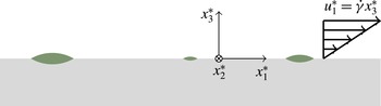
All starred quantities are dimensional in the following general mixed boundary value formulation for our problem of interest. The formulation encompasses all kinds of distributions and shapes of reactive patches:
 $$\begin{eqnarray}\displaystyle & \displaystyle D{\rm\nabla}_{x^{\ast }}^{2}C^{\ast }-\dot{{\it\gamma}}x_{3}^{\ast }\frac{\partial C^{\ast }}{\partial x_{1}^{\ast }}=0, & \displaystyle\end{eqnarray}$$
 $$\begin{eqnarray}\displaystyle & \displaystyle D\frac{\partial C^{\ast }}{\partial x_{3}^{\ast }}=kC^{\ast }\quad \text{on the reactive boundary (see figure 1)}, & \displaystyle\end{eqnarray}$$
 $$\begin{eqnarray}\displaystyle & \displaystyle \frac{\partial C^{\ast }}{\partial x_{3}^{\ast }}=0\quad \text{ on the inert boundary (see figure 1)}. & \displaystyle\end{eqnarray}$$
The dimensional concentration field
 $C^{\ast }$
obeys the advection–diffusion equation in the bulk and satisfies mixed boundary conditions over the porous surface, with reaction over the disks and no flux everywhere over the wall. The wall-normal direction is denoted by
 $x_{3}^{\ast }$
and the wall-parallel directions by
 $x_{1}^{\ast },x_{2}^{\ast }$
, as shown in figure 1. The area-averaged flux,
 $S^{\ast }$
, in such a system is given by the integral of the normal gradient of the field over the reactive disks:
 $$\begin{eqnarray}S^{\ast }=\frac{D}{A^{\ast }}\int \frac{\partial C^{\ast }}{\partial x_{3}^{\ast }}\,\text{d}A^{\ast }.\end{eqnarray}$$
Reactive disks embedded in a non-reactive wall in an unbounded surface submerged in a shear flow.

We proceed to make all equations dimensionless with the length scale of the disk radius
 $a$
and diffusion time scale
 $a^{2}/D$
. The concentration is made dimensionless with an, as yet unspecified, area-averaged surface concentration
 $\langle C^{\ast }\rangle$
, which we shall discuss for specific configurations as we proceed. The presence of shear flow and first-order surface reaction gives rise to two dimensionless parameters, the Péclet (
 $Pe$
) and Damköhler (
 ${\it\kappa}$
) numbers:
 $$\begin{eqnarray}\mathit{Pe}=\frac{\dot{{\it\gamma}}a^{2}}{D},\quad {\it\kappa}=\frac{ka}{D}.\end{eqnarray}$$
The Sherwood number (Nusselt number in the case of heat transfer) is a dimensionless measure of the area-averaged mass flux in such problems. It should be noted that the convective flux through the disk is zero. For a disk of dimensionless area
 $A$
and dimensionless concentration
 $C$
, the Sherwood number is defined as
 $$\begin{eqnarray}Sh=\frac{1}{A}\int _{\mathit{disk}}\frac{\partial C}{\partial x_{3}}\,\text{d}A.\end{eqnarray}$$
The Sherwood number is a function of
 $(\mathit{Pe},{\it\kappa})$
and the area fraction of disks. Disks can be isolated or finite in number, and we refer to either of these cases with the phrases ‘unbounded domain’ or ‘isolated’ in the remainder of this text. When the disks are distributed periodically, we refer to the case as ‘periodic’ henceforth. When the distribution of disks is randomly disordered but periodic, we refer to it by simply ‘random’ or ‘disordered’.
Juhasz & Deen (Reference Juhasz and Deen1991) used the finite element method to analyse a related problem where the flow domain was 2-D and unbounded only in the flow direction. The concentration field was independent of the vorticity direction (
 $x_{2}$
) and the reactive regions were periodic segments on the
 $x_{1}$
axis. The flow field was assumed to be unidirectional and to have a general algebraic form, as the primary goal was to show that the local Péclet number affects the Sherwood number. They also performed experiments to this effect (Juhasz & Deen Reference Juhasz and Deen1993). This exposed the shortcomings of the existing contemporary analysis of a series of problems related to mass transport to reactive spots in a non-adsorbing solid surface, where the Sherwood number was calculated using the stagnant-film approximation around the reactive region, i.e.
 $\mathit{Pe}=0$
(Nanis & Kesselman Reference Nanis and Kesselman1971; Reller, Kirowa-Eisner & Gileadi Reference Reller, Kirowa-Eisner and Gileadi1982; Dudukovic & Mills Reference Dudukovic and Mills1985). Conventional wisdom (Herskowitz, Carbonell & Smith Reference Herskowitz, Carbonell and Smith1979, among many others) suggests that the mass transfer rate, when only a fraction of the surface is reactive, is related to that in the case where the entire surface participates in reaction, through the area fraction of the reactive regions. In particular, the per-area flux in both cases is the same, and proportional to the reaction rate. Juhasz & Deen (Reference Juhasz and Deen1991) correctly anticipated the limitation that this ansatz is valid only in the case of reaction-limited transport at the microscale, by showing numerically that the Péclet number influences the interactions between the reacting sites. We shall emphasize this important distinction at greater depth in §§ 3.2 and 3.4. Juhasz & Deen (Reference Juhasz and Deen1991) thus made a necessary qualitative leap in understanding the microscale transport. However, their problem was for a simplified geometry where interactions in the vorticity direction were discarded. These interactions are found to affect the Sherwood number in an important manner (§§ 2, 3). In comparison, we provide concrete expressions to evaluate the Sherwood number in various configurations of reactive domains in a fully 3-D set-up. Veran, Aspa & Quintard (Reference Veran, Aspa and Quintard2009) and Introini, Quintard & Duval (Reference Introini, Quintard and Duval2011) also studied advection–diffusion over a heterogeneous surface, albeit in a laminar boundary layer flow regime. The surface was assumed to be rough and to have a spatially varying reaction rate, which is different from our model. Using a domain decomposition technique, the flow field and surface parameters on the scale of the roughness were linked to effective properties on the scale of the fluid domain, thus demonstrating numerically that a surface with effective homogeneous properties can replace the rough surface at an effective surface position. As mentioned before, we go a step further and provide closed-form expressions for the effective surface properties.
Considering the scope of applications of our problem discussed so far, it is surprising to note that very little quantitative progress towards understanding and obtaining continuum models has been made other than the preliminary efforts of Juhasz & Deen (Reference Juhasz and Deen1991), Veran et al. (Reference Veran, Aspa and Quintard2009) and Introini et al. (Reference Introini, Quintard and Duval2011). Mixed boundary problems of the type (1.1a
–
c
) have also been studied previously (Stone Reference Stone1989; Phillips Reference Phillips1990). In particular, Phillips developed perturbation expansions using the fundamental solution corresponding to (1.1a
–
c
) as the ‘outer’ solution for the flux to the disk in the diffusion-limited regime (
 ${\it\kappa}=\infty$
). Perhaps, the mathematically closest work to this study is that of Lucas, Sipcic & Stone (Reference Lucas, Sipcic and Stone1997), who used integral equations to solve a related problem where there is a source flux in the form of a bulk reaction instead of the convective flux due to shear flow. One can draw many parallels between the role of bulk reaction and that of a shear flow from Lucas et al. (Reference Lucas, Sipcic and Stone1997) and our numerical results, although the underlying physics is somewhat different. Our analysis formally follows the problem-solving procedures used in such studies.
To solve (1.1a
–
c
), we borrow analytical techniques from Stone (Reference Stone1989), who worked on an integral-equation-based approach to find the heat flux to a circular flush-mounted hot-plate anemometer in shear flow. This problem is mathematically equivalent to our problem in the single isolated disk setting, but, again, only in the diffusion-limited regime (large reaction rate). We also use a fundamental solution in § 2 to obtain a boundary integral solution to the concentration field for a general distribution of isolated reactive disks. We refer to this fundamental solution as the half-space Green’s function (or simply the Green’s function) due to the existence of the planar porous boundary supporting the upper half-space where the fluid flows. The half-space Green’s function has anisotropic asymptotic properties which provide insights about the length scales of the transport process. We also develop an expression for the functional dependence of the Sherwood number on
 $({\it\kappa},Pe)$
using traditional approximations existing in the field of reaction engineering, namely the law of additive resistances (Bartholomew & Farrauto Reference Bartholomew and Farrauto2011). This is an extension of similar results by Shah et al. (Reference Shah, Fitzgibbon, Narsimhan and Shaqfeh2013) to approximate the Sherwood number. The new approximation is valid over the entire range of the Péclet number.
Once the concentration field is completely determined, we can visualize the 3-D plume or wake structure that forms downstream of a disk. This wake is a concentration depletion region that develops over a finite area disk. We further derive a series of non-trivial results for the area-averaged flux in various distributions of disk configurations, explained by the wake–wake interactions between disks. This forms the core of the effective medium theory, which is ultimately developed by studying disk–disk interactions in a disordered distribution of disks in the ensuing sections.
Sangani & Behl (Reference Sangani and Behl1989) developed fundamental solutions to the periodic Stokes flow and the steady-state diffusion equation. Unlike our case, Sangani and Behl solved for effective bulk diffusivity in a medium with a planar periodic dispersion of identical surface-reactive spheres. Using the multipoles of the fundamental solution, they developed a series solution for the concentration field that is consistent with the Brinkman theory for the ‘slip’ concentration defined in terms of the area fraction and rate constant. In this work, we also develop the fundamental solution to the problem of mass transfer in shear flow to a surface with a periodic distribution of circular reactive disks. While we do not build a series solution in multipoles, for reasons that will become clear in § 2.3, we use a renormalization technique in § 3 to obtain the periodic fundamental solution. We refer to this solution as the periodic half-space Green’s function, or simply the periodic Green’s function, which leads to integral equations for the periodic concentration.
There is an important distinction between the isolated and periodic cases in that the asymptotic far-field concentration is constant for the case of isolated disks in an unbounded domain while it is affine in the wall-normal direction in the periodic case. In the periodic case, due to the infinite number of sink-like reactive disks over the surface, there must be flux supplied from the matching solution in the far field. In the matching region, the local concentration field thus displays a gradient as it approaches the heterogeneous surface, as we shall see in § 3.2.
Solution of the integral equations using the same procedure as in § 2 yields new predictions for the flux to each disk in the presence of the wall and the shear flow. The flux or Sherwood number now also depends on the disk area fraction in a meaningful manner, which is explained with our understanding of wake–wake interactions of § 2.
In § 4, we find the ensemble average Sherwood number for a random distribution of disks using periodic boundary conditions to model an unbounded surface. The concentration profile in the wall-normal direction displays a length scale, the slip length, over which diffusion and reaction balance each other on the microscale. Outside of the slip length, the Sherwood number appears in the far field as an effective reaction rate. Consequently, the effective reaction rate also depends on the disk area fraction and on the Péclet number, which provides us with the effective boundary condition constituting the porous/reactive surface theory.
We note that Sadhal & Tio (Reference Sadhal and Tio1991) and Tio & Sadhal (Reference Tio and Sadhal1992) used the method of superposition with repeated corrections to solve for the effect of the area fraction of contacts on the constriction resistance. Our strategy to solve for the leading-order effect is, in principle, equivalent to this method. In § 5, to obtain an approximation to the periodic concentration field, we develop a perturbation series in vanishing disk area fraction starting with the isolated disk concentration field. This determines the nature of the long-range interaction between the disks, but is inadequate to understand the physics at large area fractions. However, with the aid of the method of resistances we propose an approximation method that converts the Sherwood number in the unbounded or ‘zero’ areal fraction case to that for finite areal concentration. We conclude with the details of the effective medium theory in § 7 and an appendix complete with necessary derivations and proofs.
It should be noted that throughout this work we assume circular uniformly surface-reactive disks and rectangular lattices for convenience of analysis. However, the equations for the concentration field are general purpose and free from such constraints. Analogous problems can be posed in, and the results of our work are easily translated to, the case of heat transfer, as is evident from the form of the governing equations and examples mentioned previously.
2. Isolated disks in an unbounded domain
2.1. Fundamental solution
As mentioned in the introduction, our isolated disk problem is equivalent to that studied by Stone (Reference Stone1989) in the diffusion-limited regime (
 ${\it\kappa}\rightarrow \infty$
). We treat the film surface as a disk embedded in a planar surface with concentration as the field variable. We consider the simplest form of our problem (2.1a
–
d
), where the film surface has a first-order reaction and the far-field concentration is normalized to one, i.e. we choose the far-field constant concentration to make (1.1a
–
c
) dimensionless. Denoting all relevant quantities pertaining to this case by the subscript ‘
 $u$
’,
 $$\begin{eqnarray}\displaystyle & \displaystyle {\rm\nabla}_{x}^{2}C_{u}-\mathit{Pe}\,x_{3}\frac{\partial C_{u}}{\partial x_{1}}=0, & \displaystyle\end{eqnarray}$$
 $$\begin{eqnarray}\displaystyle & \displaystyle \frac{\partial C_{u}}{\partial x_{3}}={\it\kappa}C_{u}\quad \text{at }\boldsymbol{x}\in \mathscr{P}, & \displaystyle\end{eqnarray}$$
 $$\begin{eqnarray}\displaystyle & \displaystyle \frac{\partial C_{u}}{\partial x_{3}}=0\quad \text{at }\boldsymbol{x}\in \mathscr{W}, & \displaystyle\end{eqnarray}$$
 $$\begin{eqnarray}\displaystyle & \displaystyle C_{u}\rightarrow 1\quad \text{as }\Vert \boldsymbol{x}\Vert \rightarrow \infty . & \displaystyle\end{eqnarray}$$
 $x$
means that the Laplacian operator is expressed in the
 $\boldsymbol{x}$
coordinates. The concentration is denoted by
 $C_{u}$
. The wall-normal direction is denoted by
 $x_{3}$
while the in-plane Cartesian directions are associated with
 $x_{1}$
and
 $x_{2}$
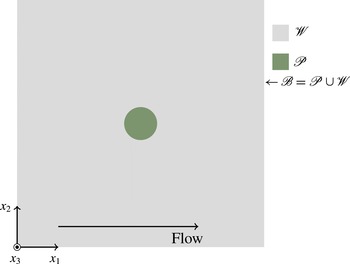
, as seen in figure 2. The disk surface,
 $\mathscr{P}$
, is embedded in the surrounding wall,
 $\mathscr{W}$
. This general problem specification allows us to treat disks of any shape. Let
 ${\it\delta}^{2}(\boldsymbol{x}_{s}-\boldsymbol{y}_{s})$
denote the Dirac delta function in two dimensions, where
 $\boldsymbol{x}_{s}=(x_{1},x_{2})$
and the source is at
 $\boldsymbol{y}_{s}=(y_{1},y_{2})$
. Similarly, let the Dirac delta function in three dimensions be denoted by
 ${\it\delta}^{3}(\boldsymbol{x}-\boldsymbol{y})$
, where
 $\boldsymbol{x}=(\boldsymbol{x}_{s},x_{3})$
and
 $\boldsymbol{y}=(\boldsymbol{y}_{s},y_{3})$
. Points bound to the surface
 $\mathscr{B}=\mathscr{W}\cup \mathscr{P}$
are denoted by a subscript
 $b$
. Thus,
 $\boldsymbol{x}_{b}=(\boldsymbol{x}_{s},0)$
and
 $\boldsymbol{y}_{b}=(\boldsymbol{y}_{s},0)$
. As discussed in the introduction, we devise a boundary element method which uses the Green’s function,
 $G_{u}$
, that satisfies the adjoint problem
 $$\begin{eqnarray}\displaystyle & \displaystyle {\rm\nabla}_{x}^{2}G_{u}+\mathit{Pe}\,x_{3}\frac{\partial G_{u}}{\partial x_{1}}=-{\it\delta}^{3}(\boldsymbol{x}-\boldsymbol{y}), & \displaystyle\end{eqnarray}$$
 $$\begin{eqnarray}\displaystyle & \displaystyle \frac{\partial G_{u}}{\partial x_{3}}=0\quad \text{at }\boldsymbol{x}\in \mathscr{B}, & \displaystyle\end{eqnarray}$$
 $$\begin{eqnarray}\displaystyle & \displaystyle G_{u}\rightarrow 0\quad \text{as }\Vert \boldsymbol{x}\Vert \rightarrow \infty . & \displaystyle\end{eqnarray}$$
Top view of an isolated disk
 $\mathscr{P}$
embedded in a wall
 $\mathscr{W}$
in an unbounded surface
 $\mathscr{B}$
with shear flow of strength
 $\dot{{\it\gamma}}$
over it.

To obtain the Green’s function, we carry out a Fourier transform of the governing equations in the
 $x_{1}$
and
 $x_{2}$
directions and solve the corresponding differential equation for the transformed variable in the wavenumber space,
 $k_{1}$
and
 $k_{2}$
. The field at
 $\boldsymbol{x}$
due to a singularity at
 $\boldsymbol{y}_{b}$
bound to
 $\mathscr{B}$
is given by
 $$\begin{eqnarray}\displaystyle \displaystyle & & \displaystyle G_{u}(\boldsymbol{x}\mid \boldsymbol{y}_{b};Pe)=\frac{1}{(2{\rm\pi})^{2}}\int _{-\infty }^{\infty }\int _{-\infty }^{\infty }\frac{-\text{Ai}(s)}{\text{Ai}^{\prime }(s_{0})(\text{i}\,\mathit{Pe}\,k_{1})^{1/3}}\text{e}^{-\text{i}\boldsymbol{k}\boldsymbol{\cdot }(\boldsymbol{x}_{s}-\boldsymbol{y}_{s})}\,\text{d}k_{1}\,\text{d}k_{2},\nonumber\\ \displaystyle & & \displaystyle \qquad \displaystyle \text{where }s=\frac{k^{2}+\text{i}\,\mathit{Pe}\,k_{1}x_{3}}{(\text{i}\,\mathit{Pe}\,k_{1})^{2/3}},s_{0}=\frac{k^{2}}{(\text{i}\,\mathit{Pe}\,k_{1})^{2/3}};k^{2}=(k_{1}^{2}+k_{2}^{2}).\end{eqnarray}$$
The reaction rate and the magnitude of the wavenumber are denoted by the same symbol,
 $k$
, so the meaning of
 $k$
should be interpreted with context throughout this work. A complete derivation of our Green’s function is provided in § A.1. Stone (Reference Stone1989) followed the same procedure but derived a Green’s function for a planar source
 ${\it\delta}^{2}(\boldsymbol{x}_{b}-\boldsymbol{y}_{b})$
on
 $\mathscr{B}$
. It is readily recovered from the free-space Green’s function (2.3) by restricting both
 $x_{3}$
and the source
 $y_{3}$
to
 $\mathscr{B}$
. We formulate the boundary integral equation for
 $C_{u}$
in the standard convolution form, as derived in § A.4:
 $$\begin{eqnarray}C_{u}(\boldsymbol{x})=1-{\it\kappa}\int _{\mathscr{P}}G_{u}(\boldsymbol{y}_{b}\mid \boldsymbol{x};Pe)C_{u}(\boldsymbol{y}_{b})\,\text{d}A(\boldsymbol{y}_{b}),\end{eqnarray}$$
where
 $\boldsymbol{y}_{b}$
is a dummy variable for integration bound to
 $\mathscr{B}$
. By substituting (2.1b
) in (1.4), we obtain a simple integral representation for the Sherwood number in the case of isolated disks in an unbounded domain:
 $$\begin{eqnarray}Sh_{u}({\it\kappa},Pe)=\frac{1}{|\mathscr{P}|}\int _{\mathscr{P}}{\it\kappa}C_{u}(\boldsymbol{x}_{b})\,\text{d}A(\boldsymbol{x}_{b}).\end{eqnarray}$$
The solution method for (2.4)–(2.5) has the following steps:
-
(1) solve (2.4) for
 $C_{u}(\boldsymbol{x}_{b})$
on
$\mathscr{P}$
by setting
$x_{3}=0$
;
-
(2) obtain
$Sh_{u}({\it\kappa},Pe)$
using (2.5); -
(3) generate
$C_{u}(\boldsymbol{x})$
in the bulk from (2.4).


It should be noted that (2.4) is a Fredholm integral equation of the second kind, and accepts a unique continuous solution in the form of a Liouville–Neumann series. However, the infinite series is computationally intractable in this case and is not convergent for large
 ${\it\kappa}$
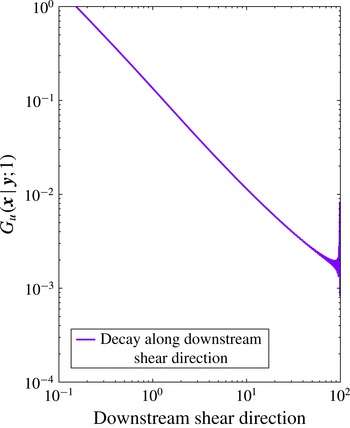
. In fact, there are several computational issues associated with evaluating the Green’s functions in (2.3). The ‘planar’ Green’s function,
 $\bar{G}_{u}=G(\boldsymbol{x}_{b}\mid \boldsymbol{y}_{b};Pe)$
, in step (1) of the method has an integrable singularity of the type
 $1/\Vert \boldsymbol{x}_{b}-\boldsymbol{y}_{b}\Vert$
. As illustrated by Stone (Reference Stone1989), we subtract this singularity from the planar Green’s function and write
 $\bar{G}_{u}=(\bar{G}_{u}-1/(2{\rm\pi}\Vert \boldsymbol{x}_{b}-\boldsymbol{y}_{b}\Vert ))+1/(2{\rm\pi}\Vert \boldsymbol{x}_{b}-\boldsymbol{y}_{b}\Vert )$
. The difference in the brackets converges fast in the Fourier domain as the Fourier coefficient
 $G_{\boldsymbol{k}}^{u}=1/((2{\rm\pi})^{2}k)$
in
 $\lim k\rightarrow \infty$
, which is the Fourier transform of
 $1/(2{\rm\pi}\Vert \boldsymbol{x}_{b}-\boldsymbol{y}_{b}\Vert )$
under our definition of the transform. We use a trapezoidal rule for evaluating this difference. Leaving out a small region around the singularity at
 $\boldsymbol{k}=0$
, we integrate the Fourier coefficients in that region using a Gauss integration scheme. We observe that the dependence of (2.2a
–
c
) on
 $Pe$
vanishes by rescaling the spatial coordinates with the square root of the Péclet number. This is captured in the identity
 $$\begin{eqnarray}G_{u}(\boldsymbol{x}\mid \boldsymbol{y};Pe)=\mathit{Pe}^{1/2}G_{u}(\mathit{Pe}^{1/2}\boldsymbol{x}\mid \mathit{Pe}^{1/2}\boldsymbol{y};1).\end{eqnarray}$$
Thus, we need to store only
 $G_{1}=G_{u}(\mathit{Pe}^{1/2}\boldsymbol{x}\mid \mathit{Pe}^{1/2}\boldsymbol{y};1)$
and we can recover the original Green’s function from the relation (2.6). The integral equation (2.4) is solved numerically by converting to matrix form,
 $\unicode[STIX]{x1D644}\boldsymbol{c}=\unicode[STIX]{x1D7D9}-{\it\kappa}\unicode[STIX]{x1D642}\boldsymbol{c}$
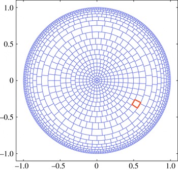
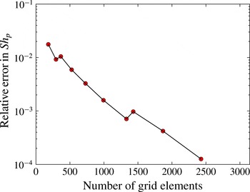
, using a collocation scheme with collocation points as centroids of elements on a mesh. This mesh for the unit disk is composed of ‘ring-sector’ elements, as highlighted in figure 3 which shows a sample mesh. To capture the large concentration gradients at the disk boundary, the meshing algorithm ensures that the radial thickness of the elements is kept small close to the boundary. The polar angular span of each element is chosen such that the elements have a good aspect ratio, approximately defined as the ratio of the radial thickness and the outer circumferential length. The elements in the interior region of the disk are also chosen to have favourable geometric properties that keep the elements regular. Effectively, the number of rings in the mesh controls the number of elements. Under this meshing scheme, we observe grid convergence for any grid with at least
 $O(1000)$
elements for a relative error of
 $10^{-3}$
in the Sherwood number (see § A.6, figure 17). Lastly, in the collocation scheme, due to the singular nature of
 $G_{u}(\boldsymbol{x}\mid \boldsymbol{y};Pe)$
, we must calculate the diagonal elements in the matrix version of the integral in (2.4) using the integral of the Green’s function over the element area. All of the matrix rows are calculated in parallel on a computing cluster and inverted using LU decomposition.
A sample mesh for a unit disk with 1331 elements.

2.2. Previous work and the method of resistances
Previously, Shah et al. (Reference Shah, Fitzgibbon, Narsimhan and Shaqfeh2013) built a semi-analytical singular perturbation theory to predict the Sherwood number for the isolated unit circular disk case based on spectral analysis. An approximate interpolation formula up to
 $O(\mathit{Pe}^{1/2})$
for the Sherwood number was derived that was accurate to
 $\mathit{Pe}\sim 100$
. Performing asymptotic scaling analysis, we improve upon this approximation and extend its validity over the entire range of the Péclet number. The key observations are as follows. First, at vanishing
 ${\it\kappa}$
, the surface concentration field over the heterogeneous surface approaches the far-field value irrespective of the value of the Péclet number:
 $$\begin{eqnarray}Sh_{u}({\it\kappa},Pe)\rightarrow {\it\kappa},\quad \text{as }{\it\kappa}\rightarrow 0.\end{eqnarray}$$
In the case of
 $\mathit{Pe}=0$
, the concentration field is harmonic, and as
 ${\it\kappa}\rightarrow \infty$
, the normal gradient over a circular disk has a well-known expression (Stone Reference Stone1989),
 $\partial C_{u}/\partial x_{3}=f({\it\rho})=(2/{\rm\pi})(1-{\it\rho}^{2})^{-1/2}$
. Thus,
 $$\begin{eqnarray}Sh_{u}(\infty ,0)=4/{\rm\pi}.\end{eqnarray}$$
With (2.7–2.8) both being upper bounds to the true Sherwood number, it is seen that the physics is reaction or kinetically limited at vanishing Damköhler number and diffusion limited at large Damköhler number. Bender & Stone (Reference Bender and Stone1993) go much further in their equations (16) and (17), where they quantify the two asymptotic limits to
 $O({\it\kappa}^{5})$
at
 ${\it\kappa}\ll 1$
and
 $o(\ln {\it\kappa}/{\it\kappa})$
at
 ${\it\kappa}\gg 1$
respectively. However, we are only concerned with the leading-order terms for the sake of this discussion and with simple correlations in mind.
The concentration field thus has a resistance of
 $1/Sh_{u}(\infty ,0)$
(
 $={\rm\pi}/4$
for a disk shape) from the far field to the disk and a resistance of
 $1/{\it\kappa}$
across the disk. The sum of these two resistances is approximately the effective resistance
 $1/Sh_{u}({\it\kappa},0)$
. This is referred to as the ‘principle of adding the global resistances’ (for example, see Roberts Reference Roberts, Rylander and Greenfield1976). Consequently, for a reactive region of arbitrary shape,
 $$\begin{eqnarray}\frac{Sh_{u}({\it\kappa},0)}{Sh_{u}(\infty ,0)}\approx \frac{{\it\kappa}}{Sh_{u}(\infty ,0)+{\it\kappa}}.\end{eqnarray}$$
It can be observed that the left-hand side is
 $O({\it\kappa})$
as
 ${\it\kappa}\rightarrow 0$
and
 $O(1)$
for
 ${\it\kappa}\rightarrow \infty$
. The approximation leading to (2.9) has been historically widely used in transport phenomena and reaction engineering (Bartholomew & Farrauto Reference Bartholomew and Farrauto2011).
To bridge this approximation to the large-Péclet-number regime in the case of circular disks, we generalize it so that
 $Sh_{u}({\it\kappa},Pe)/Sh_{u}(\infty ,Pe)\approx {\it\kappa}/(Sh_{u}(\infty ,Pe)+{\it\kappa})$
for all
 $Pe$
. For
 $Sh_{u}(\infty ,Pe)$
, we develop an approximate expression that interpolates between the known asymptotes,
 $Sh_{u}(\infty ,Pe)\rightarrow 4/{\rm\pi}+O(\mathit{Pe}^{1/2})$
as
 $\mathit{Pe}\rightarrow 0$
(Phillips Reference Phillips1990) and
 $Sh_{u}(\infty ,Pe)\rightarrow 0.6865\mathit{Pe}^{-1/3}$
as
 $\mathit{Pe}\rightarrow \infty$
. The latter value is the well-known Graetz–Lévêque limit for the boundary layer problem of mass transport to a perfectly absorbing substrate in shear flow. Using techniques described in Churchill & Usagi (Reference Churchill and Usagi1972), we obtain the following formula which matches the two asymptotes up to leading order in
 $Pe$
at both limits:
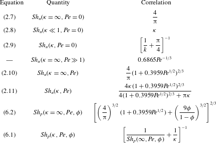
 $$\begin{eqnarray}\frac{Sh_{u}(\infty ,Pe)}{4/{\rm\pi}}\approx (1+0.3959\mathit{Pe}^{1/2})^{2/3}.\end{eqnarray}$$
This gives rise to the following approximation for the Sherwood number:
 $$\begin{eqnarray}Sh_{u}({\it\kappa},Pe)\approx \frac{4{\it\kappa}(1+0.3959\mathit{Pe}^{1/2})^{2/3}}{4(1+0.3959\mathit{Pe}^{1/2})^{2/3}+{\rm\pi}{\it\kappa}}.\end{eqnarray}$$
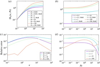
Figure 4 shows that the Sherwood number of the approximation (2.11) is in excellent agreement (
 ${<}3\,\%$
error) with the Sherwood number predicted by the exact boundary element results (2.4) at all Péclet and Damköhler numbers. The boundary element simulations were performed with 1331 mesh elements for the unit circular disk.
The Sherwood number and its approximation based on the method of resistances (MoR) (2.11) for an isolated disk is plotted (a) versus the Damköhler number for varying Péclet number and (b) versus the Péclet number for varying Damköhler number. The approximation is in good agreement with the exact Sherwood number obtained from the boundary integral solution. The relative error of using the method of resistances instead of the exact solution is plotted in (c) versus the Damköhler number for varying Péclet number and (d) versus the Péclet number for varying Damköhler number. The Damköhler number is varied from 0.1 (reaction limited) to large values such as 300 (diffusion limited) and the Péclet number from 0.001 (no flow) to 100 (strong shear).

The effect of the Péclet number at a fixed Damköhler number is subtle in the regime of vanishing Péclet number (see figure 4
b). Previous work by Shah et al. (Reference Shah, Fitzgibbon, Narsimhan and Shaqfeh2013) indicates an
 $O(\mathit{Pe}^{1/2})$
growth in the Sherwood number at all Damköhler numbers, up to moderate Péclet number (
 $O(1)$
). The current work extends the theory to (2.11), which is valid at all orders in the Péclet number. Certainly, the slopes of the curves for the Sherwood number at large Péclet number approach the Graetz–Lévêque limiting value of
 $1/3$
, indicative of the
 $\mathit{Pe}^{1/3}$
scaling. It should be noted that since the Sherwood number has a limiting asymptotic value at large
 ${\it\kappa}$
, the results of Stone (Reference Stone1989) are reproduced by setting
 ${\it\kappa}$
sufficiently large in the boundary element simulations.
It is evident from the logarithmic plot in figure 4(a) that independent of the Péclet number, all curves have a slope of unity at vanishing Damköhler number. This confirms the observation of (2.7) that the transport is kinetically limited and, thus, the Sherwood number equals the value of the Damköhler number in that regime. As the Damköhler number is increased, for every Péclet number, the Sherwood number grows asymptotically to the value in (2.10). This is represented by the plateau in the curves at large
 ${\it\kappa}$
.
In the limit of large Damköhler number, the Sherwood number follows the expression in (2.10), where the problem reduces to that of heat transfer from an isothermal disk in a high-shear flow. Many researchers (Lévêque Reference Lévêque1928; Reiss & Hanratty Reference Reiss and Hanratty1963) have looked at the heat transfer problem for the case of an isothermal rectangular strip and obtained higher-order corrections to their Sherwood number expressions by analysing the heat transfer in the boundary layers on the edges of the strip. Phillips (Reference Phillips1990) extended the same analysis to determine the contributions to flux from different regions of the isothermal disk. In particular, for
 $\mathit{Pe}\ll 1$
, the side edges of a disk of thickness scaling as
 $\mathit{Pe}^{-1/2}$
have stream-wise diffusion balancing the convection, resulting in a convective length scale that scales as
 $\mathit{Pe}^{-1/2}$
. Thus, the concentration gradient scales as
 $\mathit{Pe}^{1/2}$
, and, consequently, the side-edge regions contribute a flux of
 $O(1)$
. Similarly, the central region of the disk is of size
 $O(1)$
, over which the concentration gradients scale as
 $\mathit{Pe}^{1/2}$
at small Péclet number. Thus, the total Sherwood number is
 $O(1)+O(\mathit{Pe}^{1/2})$
, which matches the small-Péclet asymptote of (2.10). At
 $\mathit{Pe}\gg 1$
, the depletion region over the central region of the disk scales in length as
 $\mathit{Pe}^{-1/3}$
, so the flux contribution is
 $O(\mathit{Pe}^{1/3})$
. At large shear, the leading and trailing edges also contribute a flux of
 $O(\mathit{Pe}^{-1/6})$
. Thus, the total Sherwood number at large Péclet number is
 $O(\mathit{Pe}^{1/3})+O(\mathit{Pe}^{-1/6})$
, matching the Graetz–Lévêque asymptote of (2.10).
The existence of a finite Damköhler number at the disk introduces an extra length scale in the form of reaction transport over the disk. When
 ${\it\kappa}\rightarrow 0$
, the depletion region scales on the reaction length scale as the transport is kinetically limited. Then, the flux through the disk is of the same value as the Damköhler number to the first order. As the Damköhler number is increased, the reaction length scale becomes comparable to the convection length scale. Within the depletion region the convective flux is ‘throttled’ by the Damköhler number. Consequently, the principle of addition of local resistances applies and the Sherwood number is a harmonic sum of the Damköhler number and the convective flux to a purely adsorbing disk (2.10), resulting in the expression (2.11). With these insights into the fully 3-D nature of the single-disk problem, we explore interesting concentration wake structures that develop downstream of a disk.
2.3. Wake structure
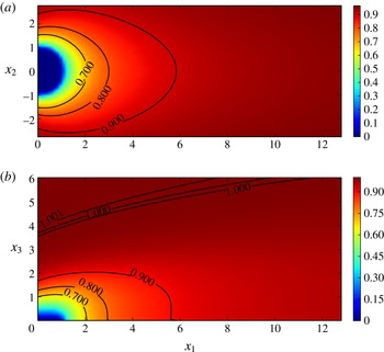
In figure 5(a,b), we plot the isotherms of the concentration field on the surface around the disk and on a vertical slice passing through the centre of the disk. The contours correspond to the case of moderate Péclet number in the diffusion-limited regime. We see in figure 5(a) that a wake is formed around the disk. It is a concentration depletion region caused by the presence of the disk. The wake has a full 3-D structure and scales in the normal direction on a combination of the reaction length scale and the convection length scale, visible in figure 5(b).
The 3-D wake structure that forms around a disk for
 ${\it\kappa}=300$
and
 $\mathit{Pe}=2$
: (a) the wake extends downstream in the shear direction,
 $x_{1}$
, as displayed by isolines of concentration over the wall (in the
 $x_{1}{-}x_{2}$
plane at
 $x_{3}=0$
); (b) isolines in the vertical plane through the disk centre (
 $x_{1}{-}x_{3}$
plane at
 $x_{2}=0$
) show the depletion layer thickness over the disk. Contours in the far field grow with distance in the shear direction.

The exact structure of the wake becomes apparent upon analysis of the fundamental solution (2.3), which formally contains all of the 3-D information about the field. This information can be accessed by expanding the boundary integral equation (2.4) into a series of multipoles of the fundamental solution
 $G_{u}$
. The standard procedure is to express the higher-order multiples in terms of lower-order ones using the differential equation, so that a finite number of coefficients can be determined using a collocation scheme to match the numerical solution with the expansion. In this case, however, the Fourier coefficients decay as
 $1/k$
. Consequently, evaluation of the partial derivatives in higher-order multipoles using term-wise differentiation does not yield convergent integrals. Nonetheless, we find that curtailing the expansion to just the monopole is still informative. For an isolated disk centred at
 $\mathbf{0}$
,
 $$\begin{eqnarray}C_{u}(\boldsymbol{x})\approx 1-{\rm\pi}G_{u}(\mathbf{0}\mid \boldsymbol{x};Pe)Sh_{u}.\end{eqnarray}$$
As the fundamental solution has a scale-invariance property (2.6), an algebraic decay in any direction or part of the domain will be of the type
 $1/\Vert \boldsymbol{x}-\boldsymbol{y}\Vert$
. The Green’s function indeed decays algebraically on the length scale of the disk radius, at points
 $(x_{1},a,0)$
directly downstream of the source singularity
 $(y_{1},a,0)$
:
 $$\begin{eqnarray}G_{u}\sim \frac{1}{(x_{1}-y_{1})}\quad \text{for }(x_{1}-y_{1})\gg 1.\end{eqnarray}$$
We refer the interested reader to § A.3 for the derivation of (2.13). From (2.12), the concentration in the far field is
 $C_{u}(\boldsymbol{x})=O(f(Pe)/\Vert \boldsymbol{x}\Vert )$
, with
 $f(Pe)\sim O(\mathit{Pe}^{1/3})$
at large
 $Pe$
. Consequently, as the Péclet number increases, the wake becomes elongated in the downstream shear direction. The wake thickness in the vorticity direction (
 $x_{2}$
) is determined by the diffusion in that direction, so its thickness is visibly narrower than the wake length in the shear direction at large Péclet number (figure 5
a). In the standard Graetz boundary layer problem of mass transfer from a semi-infinite plate to the shear flow, the isotherms in figure 5(b) would extend indefinitely downstream in the shear direction. As we only have a finite disk area, the isotherms eventually bend and extinguish on the wall, which corresponds to a finite length of the wake.
In the case of a multi-disk problem, the 3-D wakes around each disk interact with each other to form complex structures and affect the total transport to each disk. We investigate the specific case of a two-disk system to gain insight into the mechanism of disk–disk interactions and its implications for more complex systems of disks.
2.4. The two-disk system
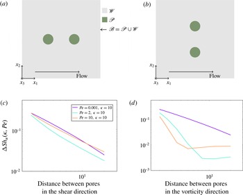
As remarked previously, we can solve the concentration field for disks of arbitrary shapes, or even a system of disjoint disks, using (2.4). Taking advantage of this capability, we calculate the area-averaged Sherwood number for the case of two disks of unit radius kept in two distinct configurations. The first configuration is that of two disks aligned perfectly in the shear direction and the second one is that of two disks aligned in the vorticity direction. In figure 6(c,d) we plot the difference between the Sherwood number for a single disk and the Sherwood number in the two-disk problem against the separation distance between the two disks.
The difference between the Sherwood number for a single disk and the two-disk problem, for two different configurations, with increasing separation distance shows distinct trends. Displayed first are schematics of (a) two disks aligned in the shear direction and (b) two disks aligned in the vorticity direction. The Sherwood number in the two-disk problem approaches the single-disk Sherwood number (c) inversely with the separation distance between the two disks when aligned in the shear direction and (d) much faster than the inverse of the separation distance between the two disks when aligned in the vorticity direction.

We notice that at large distances of separation between the two disks in either configuration, the Sherwood number approaches the single-disk flux asymptotically, though with different rates. When the two disks are aligned in the shear direction, the first reflection of the disk upstream at the disk downstream has a strength proportional to the inverse of the separation distance between the two disks (see (2.13)). Subsequently, the two disks share the depletion region and the gradient above the disk downstream is reduced in strength proportional to the separation distance. In other words, the disks share the wakes, and the Sherwood number for this case is always smaller than the single-disk one. The effect of sharing the wakes is reflected in the linear decay with unity slope in figure 6(c) over a large range of the Péclet number.
In comparison, the difference in the Sherwood number when the disks are aligned in the vorticity direction does not display a linear profile at large Péclet number. For moderate separation scales that depend on the Péclet number and are comparable to the disk radius, the profile displays a faster decay than the inverse of the separation distance. This is explained by the fact that the wake for a single disk is thinner in the vorticity direction than in the shear direction. Therefore, the disks aligned in the vorticity direction do not share much of their depletion region unless they are sufficiently close or the Péclet number is vanishingly small. This knowledge of wake structures and disk–disk interactions is central in the analysis of a periodic distribution of disks in the next section.
3. Periodic array of disks
3.1. The fundamental periodic solution
Using the same strategy as in the previous section, we study the case of transport to periodic planar arrays of disks with surface reaction. Such a distribution of disks is modelled by first tiling the surface
 $\mathscr{B}$
into identical units or boxes
 $\mathscr{B}_{\boldsymbol{n}}$
, so that they have the same shape and size footprint. The reactive region
 $\mathscr{P}_{\boldsymbol{n}}$
in each box can be disordered but is identical across boxes, ensuring periodicity. Similarly, the half-space
 $\mathscr{V}=\{x_{3}\geqslant 0\}$
can be tessellated into identical half-volumes
 $\mathscr{V}_{\boldsymbol{n}}$
, each placed on the respective bottom faces
 $\mathscr{B}_{\boldsymbol{n}}$
. It is obvious that the notation from the previous section easily accommodates the periodic nature of this case through the use of the subscript ‘
 $n$
’. For example,
 $\mathscr{B}_{\boldsymbol{n}}=\mathscr{W}_{\boldsymbol{n}}\cup \mathscr{P}_{\boldsymbol{n}}$
and
 $\mathscr{B}=\cup \mathscr{B}_{\boldsymbol{n}},\mathscr{W}=\cup \mathscr{W}_{\boldsymbol{n}},\mathscr{P}=\cup \mathscr{P}_{\boldsymbol{n}}$
. The centre of each such box
 $\mathscr{B}_{\boldsymbol{n}}$
is given by lattice points
 $$\begin{eqnarray}\boldsymbol{r}_{\boldsymbol{n}}=n_{1}\boldsymbol{L}_{1}+n_{2}\boldsymbol{L}_{2}\quad (n_{1},n_{2}=0,\pm 1,\pm 2,\ldots ),\end{eqnarray}$$
where the periodic directions
 $\boldsymbol{L}_{1}$
and
 $\boldsymbol{L}_{2}$
are aligned to the surface
 $\mathscr{B}$
such that
 $\hat{x}_{3},\boldsymbol{L}_{1},\boldsymbol{L}_{2}$
form a Cartesian coordinate system. When the periodicity is in the Cartesian directions
 $x_{1}$
and
 $x_{2}$
, each box
 $\mathscr{B}_{\boldsymbol{n}}$
is a simple rectangle
 $[0,\boldsymbol{L}_{1}]\times [0,\boldsymbol{L}_{2}]$
. The area of each box is denoted by
 $|\mathscr{B}_{\boldsymbol{n}}|=\hat{x}_{3}\boldsymbol{\cdot }(\boldsymbol{L}_{1}\times \boldsymbol{L}_{2})=B_{0}$
. The area of the reactive region in each box is denoted by
 $|\mathscr{P}_{\boldsymbol{n}}|=P_{0}$
.
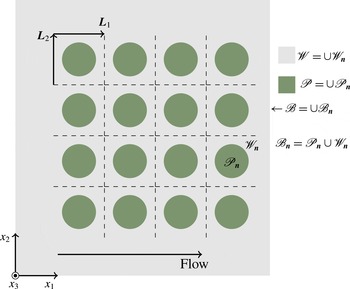
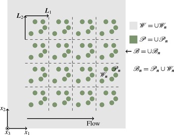
A periodic system of reactive regions
 $\mathscr{P}_{\boldsymbol{n}}$
embedded in tiled pieces of the wall
 $\mathscr{W}_{\boldsymbol{n}}$
in corresponding bounding boxes
 $\mathscr{B}_{\boldsymbol{n}}$
. A shear flow of strength
 $\dot{{\it\gamma}}$
is present in the wall-normal direction. Also illustrated are the periodicity directions
 $\boldsymbol{L}_{1},\boldsymbol{L}_{2}$
in the lattice.

Let us denote all the relevant quantities in this case with a subscript ‘
 $p$
’ indicating periodicity. Then,
 $C_{p}$
satisfies the same set of governing and boundary equations as the isolated disk problem, albeit now in each volume
 $\mathscr{V}_{\boldsymbol{n}}$
with the corresponding lattice point
 $\boldsymbol{r}_{\boldsymbol{n}}$
:
 $$\begin{eqnarray}\displaystyle & \displaystyle {\rm\nabla}_{x}^{2}C_{p}-\mathit{Pe}\,x_{3}\frac{\partial C_{p}}{\partial x_{1}}=0, & \displaystyle\end{eqnarray}$$
 $$\begin{eqnarray}\displaystyle & \displaystyle \frac{\partial C_{p}}{\partial x_{3}}={\it\kappa}C_{u}\quad \text{at }\boldsymbol{x}\in \mathscr{P}_{\boldsymbol{n}},\boldsymbol{n}\in \mathbb{Z}^{2}, & \displaystyle\end{eqnarray}$$
 $$\begin{eqnarray}\displaystyle & \displaystyle \frac{\partial C_{p}}{\partial x_{3}}=0\quad \text{at }\boldsymbol{x}\in \mathscr{W}_{\boldsymbol{n}},\boldsymbol{n}\in \mathbb{Z}^{2}. & \displaystyle\end{eqnarray}$$
A condition equivalent to (2.1d
) cannot be posed for the periodic case. The divergence theorem ensures that the flux at any wall-parallel (
 $x_{3}$
) plane is the same as the flux through a disk, which is the same as the flux at
 $x_{3}\rightarrow \infty$
. Noting that the average surface field variable is
 $\langle C_{p}\rangle (x_{3}=0)=1$
, the correct asymptotic condition for
 $C_{p}$
is given in terms of the Sherwood number and the area fraction
 $P_{0}/B_{0}$
:
 $$\begin{eqnarray}C_{p}\rightarrow 1+\frac{P_{0}}{B_{0}}Sh_{p}x_{3}\quad \text{as }x_{3}\rightarrow \infty .\end{eqnarray}$$
Here, the Sherwood number,
 $Sh_{p}$
, is identical for each reactive region
 $\mathscr{P}_{\boldsymbol{n}}$
, and is given by the expression
 $$\begin{eqnarray}Sh_{p}({\it\kappa},\mathit{Pe},{\it\phi})=\frac{1}{|\mathscr{P}_{\boldsymbol{n}}|}\int _{\mathscr{P}_{\boldsymbol{n}}}{\it\kappa}C_{p}(\boldsymbol{x}_{b})\,\text{d}A(\boldsymbol{x}_{b}),\end{eqnarray}$$
where
 ${\it\phi}$
is the area fraction of the disks as defined by
 ${\it\phi}=P_{0}/B_{0}$
. The periodic Green’s function satisfies the following set of equations:
 $$\begin{eqnarray}\displaystyle & \displaystyle {\rm\nabla}^{2}G_{p}+\mathit{Pe}\,x_{3}\frac{\partial G_{p}}{\partial x_{1}}=-{\it\delta}(x_{3}-y_{3})\left({\it\delta}^{2}(\boldsymbol{x}_{s}-\boldsymbol{y}_{s,\boldsymbol{n}})-\frac{1}{B_{0}}\right), & \displaystyle\end{eqnarray}$$
 $$\begin{eqnarray}\displaystyle & \displaystyle \frac{\partial G_{p}}{\partial x_{3}}=0\quad \text{at }\boldsymbol{x}\in \mathscr{B}_{\boldsymbol{n}}, & \displaystyle\end{eqnarray}$$
 $$\begin{eqnarray}\displaystyle & \displaystyle G_{p}\rightarrow 0\quad \text{ as }x_{3}\rightarrow \infty , & \displaystyle\end{eqnarray}$$
 $\partial \mathscr{B}_{\boldsymbol{n}}$
. Equivalently, the singularities are distributed periodically at
 $\boldsymbol{y}_{\boldsymbol{n}}=(\boldsymbol{y}_{s,\boldsymbol{n}},y_{3})$
, where
 $$\begin{eqnarray}\boldsymbol{y}_{s,\boldsymbol{n}}=\boldsymbol{y}_{s,0}+n_{1}\boldsymbol{L}_{1}+n_{2}\boldsymbol{L}_{2}\quad (n_{1},n_{2}=0,\pm 1,\pm 2,\ldots ).\end{eqnarray}$$
Thus,
 ${\it\delta}^{2}(\boldsymbol{x}_{s}-\boldsymbol{y}_{s,\boldsymbol{n}})$
is a two-dimensional periodic delta function, also known as the Dirac comb in mathematical physics (Córdoba Reference Córdoba1989).
The solution to (3.4a
–
c
) is expressed as a Fourier series because of the periodicity of the domain. To ensure that the Fourier series converges and no term is singular, we modify the source term to include a uniform background sink term
 $1/B_{0}$
. The source and the sink flux are balanced over each box
 $\mathscr{B}_{\boldsymbol{n}}$
. This modification is also referred to in the literature (Hasimoto Reference Hasimoto1959; Sangani & Behl Reference Sangani and Behl1989) as renormalization of the Green’s function.
Given the periodicity directions
 $\boldsymbol{L}_{1},\boldsymbol{L}_{2}$
, the Green’s function depends only on
 $\boldsymbol{y}_{s,0}$
, so we drop the subscript
 $\boldsymbol{n}$
for the sake of clarity. We refer the interested reader to § A.5 for a complete derivation of the periodic Green’s function, and simply quote it here for the case where the periodic singularities are bound to the surface
 $\mathscr{B}$
:
 $$\begin{eqnarray}G_{p}(\boldsymbol{x}\mid \boldsymbol{y}_{b};Pe)=\frac{1}{B_{0}}\mathop{\sum }_{k\neq 0}\frac{-\text{Ai}(s)}{\text{Ai}^{\prime }(s_{0})(\text{i}\,\mathit{Pe}\,k_{1})^{1/3}}\text{e}^{-\text{i}\boldsymbol{k}\boldsymbol{\cdot }(\boldsymbol{x}_{s}-\boldsymbol{y}_{s})},\end{eqnarray}$$
where
 $\boldsymbol{k}=(k_{1},k_{2})$
are vectors in the reciprocal lattice,
 $$\begin{eqnarray}\displaystyle & \displaystyle \boldsymbol{k}=2{\rm\pi}n_{1}\boldsymbol{l}_{1}+2{\rm\pi}n_{2}\boldsymbol{l}_{2}\quad (n_{1},n_{2}=0,\pm 1,\pm 2,\ldots ), & \displaystyle\end{eqnarray}$$
 $$\begin{eqnarray}\displaystyle & \displaystyle \text{where }\boldsymbol{l}_{1}=\frac{\boldsymbol{L}_{2}\times \hat{x}_{3}}{B_{0}},\quad \boldsymbol{l}_{2}=\frac{\hat{x}_{3}\times \boldsymbol{L}_{1}}{B_{0}}, & \displaystyle\end{eqnarray}$$
 $$\begin{eqnarray}\displaystyle & \displaystyle \text{so }\boldsymbol{k}\boldsymbol{\cdot }\boldsymbol{L}_{t}=2{\rm\pi}n_{t}\quad (t=1,2). & \displaystyle\end{eqnarray}$$
It should be noted that the area fraction affects the calculations of the Green’s function and the concentration field through (3.7b,c
). The procedures for deriving expressions for
 $G_{p}$
and
 $G_{u}$
are very similar. Not surprisingly, both have similar expressions for the Fourier modes. The periodic concentration also satisfies a Fredholm integral equation of the second kind, but with a periodic kernel:
 $$\begin{eqnarray}C_{p}(\boldsymbol{x})=1+\frac{P_{0}Sh_{p}}{B_{0}}x_{3}-{\it\kappa}\int _{\mathscr{P}_{0}}G_{p}(\boldsymbol{y}_{b}\mid \boldsymbol{x};Pe)C_{p}(\boldsymbol{y}_{b})\,\text{d}A(\boldsymbol{y}_{b}).\end{eqnarray}$$
The complete derivation for this boundary integral equation can be found in § A.6. The solution method is as follows:
-
(1) solve (3.8) for
$C_{p}(\boldsymbol{x}_{b})$
on
$\mathscr{P}_{0}$
; -
(2) obtain
$Sh_{p}({\it\kappa},\mathit{Pe},{\it\phi})$
using (3.3); -
(3) generate
$C_{p}(\boldsymbol{x})$
in the bulk as the left-hand side of (3.8).


Accurate calculation of the periodic Green’s function is again somewhat involved, and similar considerations to those at the end of § 2.1 need to be taken into account. The computation procedure is detailed in § A.2. As expected, in the limit as the box
 $\mathscr{B}_{0}$
becomes unbounded, the periodic Green’s function converges to the isolated Green’s function at points in
 $\mathscr{B}_{0}$
for a coinciding singularity inside
 $\mathscr{B}_{0}$
:
 $$\begin{eqnarray}G_{u}(\boldsymbol{x}\mid \boldsymbol{y};Pe)=\lim _{B_{0}\rightarrow \infty }G_{p}(\boldsymbol{x}\mid \boldsymbol{y};Pe).\end{eqnarray}$$
3.2. Justification of boundary condition (3.2d ), structure of the mathematical problem, and the Damköhler approximation
Clearly, from a physical standpoint, the interpretation of the boundary condition (3.2d
) requires discussion since the solution that we are seeking appears to approach infinite concentration far from the heterogeneous reactive surface. The issue lies in the fact that there is no decaying one-dimensional solution to the diffusion equation over the half-space
 $x_{3}\geqslant 0$
, with uniform reaction at
 $x_{3}=0$
. Therefore, the boundary condition (3.2d
) must represent the microscopic solution as we move far from the details of the transport at the scale of the reactive patches. This must match to the solution at an outer or macroscopic length scale – the latter length scale we shall define as
 $H$
, as illustrated in figure 8. If the outer solution can be characterized by an effective first-order surface reaction coefficient as one approaches the heterogeneous surface, then the effective boundary condition (in dimensional form) to the outer problem must be of the form
 $$\begin{eqnarray}D\frac{\partial C_{p}^{\ast }}{\partial x_{3}^{\ast }}=k_{eff}C_{p}^{\ast };\quad \lim x_{3}^{\ast }\ll H,\end{eqnarray}$$
or, more precisely, if we make lengths dimensionless with
 $H$
, defining
 ${\it\xi}=x_{3}^{\ast }/H$
,
 $$\begin{eqnarray}\frac{\partial C_{p}^{\ast }}{\partial {\it\xi}}={\it\kappa}_{o}C_{p}^{\ast };\quad \lim {\it\xi}\rightarrow 0,\end{eqnarray}$$
where
 ${\it\kappa}_{o}$
is the Damköhler number on the outer scale,
 ${\it\kappa}_{o}=k_{eff}H/D$
.
Taking a Taylor series of
 $C_{p}^{\ast }$
in outer variables and applying the effective boundary condition gives
 $$\begin{eqnarray}C_{p}^{\ast }={C_{p}^{\ast }}_{o}\left[1+{\it\kappa}_{o}{\it\xi}+\cdots \right]={C_{p}^{\ast }}_{o}\left[1+\frac{k_{eff}x_{3}^{\ast }}{D}+\cdots \right],\end{eqnarray}$$
where
 ${C_{p}^{\ast }}_{o}$
is the (constant) ‘concentration at the interface’ in the macroscale problem. It should be noted that we have identified it as the mean concentration at the surface in the microscale periodic problem (see the discussion before (3.2d
)). The mean surface concentration is a scale factor for the inner problem, and thus the matching condition (3.2d
) for a periodic array of reactive disks is equivalent to
 $$\begin{eqnarray}\left[1+\frac{k_{eff}ax_{3}}{D}+\cdots \right]=\left[1+\frac{P_{0}}{B_{0}}Sh_{p}({\it\kappa},Pe)x_{3}+\cdots \right]\end{eqnarray}$$
or
 $$\begin{eqnarray}{\it\kappa}_{eff}=\frac{k_{eff}a}{D}=\frac{P_{0}}{B_{0}}Sh_{p}({\it\kappa},\mathit{Pe},{\it\phi})={\it\phi}Sh_{p}({\it\kappa},\mathit{Pe},{\it\phi}),\end{eqnarray}$$
where
 ${\it\phi}$
is actually the areal fraction of the reactive domains on the periodic surface.
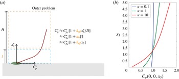
The outer problem scales on length scale
 $H$
, where the dimensionless concentration is approximately
 $1+{\it\kappa}_{eff}x_{3}+\cdots =1+{\it\kappa}_{o}{\it\xi}+\,\cdots ,$
as shown in (a). This serves as the far-field value that the concentration on the microscale asymptotes to over the distance
 $l^{\ast }$
, called the slip length. The slip length is visible in (b), where the concentration field profile
 $C_{p}(0,0,x_{3})$
exactly above the disk centre, calculated using (3.8), is plotted against
 $x_{3}$
at
 $\mathit{Pe}=0.001$
and three values of
 ${\it\kappa}$
. The slip distance appears to be weakly dependent on the Damköhler number, and the concentration field appears to reach the asymptotic value within a wall-normal distance that scales as the disk radius.

This then defines the effective dimensionless reaction rate/surface mass transfer coefficient, namely
 ${\it\kappa}_{eff}=k_{eff}a/D$
, in terms of the Sherwood number for any value of the microscale Damköhler number
 ${\it\kappa}$
and the Péclet number
 $Pe$
. In order for this mathematical structure and matching procedure to hold, we only need
 $H>l^{\ast }$
, where
 $l^{\ast }$
is the dimensional slip length or the distance at which the microproblem asymptotes to the far-field condition
 $C_{p}=C_{p}^{\ast }/{C_{p}^{\ast }}_{o}\rightarrow [1+(P_{0}/B_{0})Sh_{p}({\it\kappa},Pe)x_{3}+\,\cdots ]$
, as seen in figure 8. We calculate the dimensionless slip length
 $l=l^{\ast }/a$
as a function of
 ${\it\phi}$
,
 ${\it\kappa}$
and
 $Pe$
for periodic arrays in § 3.4 and for random reactive domains in § 4. It should be noted that the microscale to macroscale matching condition is essentially the same for random domains, and we revisit this discussion for random domains in § 4.
The value of
 ${C_{p}^{\ast }}_{o}$
and its functionality with
 ${\it\kappa}_{o}$
are determined by the complete solution of the outer problem along with the other outer boundary conditions, and, for complete generality, we do not specify these in the present study. There are obviously many different situations of interest including constant concentration and constant flux at scales of
 $O(H)$
. In general, then, the outer problem depends intrinsically on
 $k_{eff}$
. There is one caveat to this statement and that is for sufficiently large
 ${\it\kappa}_{o}$
, where the outer problem is diffusion limited and
 $$\begin{eqnarray}C_{p}^{\ast }={C_{p}^{\ast }}_{o}\rightarrow 0;\quad \lim {\it\xi}\rightarrow 0.\end{eqnarray}$$
In this case, the outer problem can be solved independently of the inner problem via the application of the appropriate Dirichlet condition above, and thus the flux at the interface can be calculated from a geometric problem at the outer scale alone. A quantitative estimate of the outer Damköhler number is highly relevant, but generally difficult since we need to estimate
 $k_{eff}$
. There is one limit in which this can be done easily and that is when the reaction is limiting at the microscale, i.e.
 ${\it\kappa}\ll 1$
. This is the limiting case originally considered by Juhasz & Deen (Reference Juhasz and Deen1991), and (incorrectly) assumed to be uniformly true by Herskowitz et al. (Reference Herskowitz, Carbonell and Smith1979). In this case, the concentration is constant, to leading order in small
 ${\it\kappa}$
, throughout the microscale region (e.g. cf. (2.4) and (3.8)). Perturbation theory for small
 ${\it\kappa}$
then gives, regardless of
 ${\it\phi}$
,
 $$\begin{eqnarray}{\it\phi}Sh_{p}({\it\kappa},\mathit{Pe},{\it\phi})\approx {\it\phi}{\it\kappa},\end{eqnarray}$$
and thus
 $$\begin{eqnarray}\frac{k_{eff}a}{D}\approx {\it\phi}{\it\kappa},\end{eqnarray}$$
which is the mathematical statement that the effective reaction rate is the areal fraction times the reaction rate in each reactive domain (and is thus a material property, independent of the geometric details). In this case, and in this case only,
 $$\begin{eqnarray}{\it\kappa}_{o}\approx {\it\phi}{\it\kappa}\frac{H}{a}.\end{eqnarray}$$
It should be noted that we shall return to the question of estimating the size of
 ${\it\kappa}_{o}$
for values of
 ${\it\kappa}$
that are not small. Indeed, we demonstrate that the equation above is, under more general conditions, a gross overestimate of
 ${\it\kappa}_{o}$
primarily because of the failure of the expression
 ${\it\phi}Sh_{p}({\it\kappa},Pe)\approx {\it\phi}{\it\kappa}$
for
 ${\it\kappa}\sim O(1)$
.
3.3. Comparison between the Sherwood number in the periodic and unbounded domains
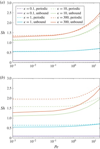
When the area fraction of disks in the periodic system is vanishingly small, (3.9) shows that the periodic Green’s function is close in value to the isolated Green’s function. Accordingly, we see from figure 9(a) that the Sherwood numbers in periodic and unbounded domain cases are close in value over a wide range of the Péclet and Damköhler numbers. A peculiar characteristic of the curves in figure 9(a) is that at all Damköhler numbers, the periodic case Sherwood number (
 $Sh_{p}$
) is greater than the unbounded domain case Sherwood number (
 $Sh_{u}$
) at vanishing Péclet number. Conversely,
 $Sh_{p}<Sh_{u}$
for large values of the Péclet number. When the area fraction of disks is just an order of magnitude larger (see figure 9
b), we notice that the Sherwood number in the periodic case is significantly larger than that in the unbounded case, and over a wider range of Péclet number. In fact, the two Sherwood number curves do not meet until a Péclet number beyond the range shown on the plot.
Plot of the Sherwood number for a periodic system of single disks per bounding box with lattice lengths (a)
 ${\it\phi}=0.00126$
(
 $\boldsymbol{L}_{1}=\boldsymbol{L}_{2}=50$
) and (b)
 ${\it\phi}=0.064$
(
 $\boldsymbol{L}_{1}=\boldsymbol{L}_{2}=7$
) in comparison with the Sherwood number for an isolated single disk.

The origin of these contrasting trends in the two regimes of the Péclet number can be traced to the distinctive wake–wake interactions in the two lattice directions and their relative strengths for different Péclet numbers. We recall from § 2.4 that the wake interactions in the shear direction lead to a larger decrease in per-disk flux as compared with that in the vorticity direction. This behaviour is a direct consequence of the fact that for a single isolated disk, the wake lengthens in the shear direction and contracts in the vorticity direction with increasing Péclet number (see figure 5
a). In fact, for large Péclet number, the wakes are shared in the shear direction, as seen in figure 10(a), resulting in weaker normal concentration gradients. Consequently, the per-disk flux is smaller compared with a single isolated disk. At vanishing Péclet number, the wakes are shared in both the shear and vorticity directions. The existence of a background sink (see (3.2a
)) enforces the following constraint on the mean surface concentration:
 $\langle C_{p}\rangle (x_{3}=0)=1$
, which drives the normal gradients to be greater at small Péclet number. This opposing ‘sink effect’ eventually dominates the wake-sharing effect when the vorticity direction interactions are large enough in size, resulting in
 $Sh_{p}>Sh_{u}$
.
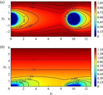
(a) Contours are plotted over a part of the region
 $\mathscr{B}_{0}$
for the case of
 ${\it\kappa}=300$
and
 $P=10$
with periodic disks (
 $\boldsymbol{L}_{1}=\boldsymbol{L}_{2}=10$
). Contours are lengthened in the shear direction,
 $x_{1}$
, and periodic. (b) Contours are plotted in the
 $x_{1}{-}x_{3}$
plane passing through the disk centre, for the case of
 ${\it\kappa}=300$
and
 $P=10$
. The isotherms depict sharing of the depletion regions in the periodic directions (
 $\boldsymbol{L}_{1}=\boldsymbol{L}_{2}=10$
). Contour growth in the far field is restricted by sharing.

Thus, for a given Damköhler number, for each area fraction there exists a unique ‘cutoff’ Péclet number where the two Sherwood numbers are equal. Conversely, there exists a unique cutoff area fraction for any given Péclet number at which the order relation between
 $Sh_{u}$
and
 $Sh_{p}$
flips. This is similar to how the first inertial effect on the drag on a periodic array of spheres differs from the Oseen approximation for drag on an isolated sphere as
 ${\it\phi}$
increases at a fixed mean flow through the periodic box (Hill, Koch & Ladd Reference Hill, Koch and Ladd2001). The cutoff Péclet number is larger at larger area fractions, as the wake-sharing phenomenon dominates only at increasingly larger values of the Péclet number. The cutoff Péclet number is nearly independent of the value of the Damköhler number, as explained later in § 6.
3.4. Slip distance and effective reaction rate
The boundary integral equation (3.8) and asymptotic condition (3.2d
) suggest that the concentration field in the periodic case decays to the asymptotic linear form (3.2d
) at a ‘slip distance’ normal to the heterogeneous surface (see the discussion in § 3.2). This is also evident from figure 10(b), as the variations in concentration isotherms decay at a distance on the order of few disk radii normal to the heterogeneous surface. The contours of figure 10(b) indicate that the peak variation from the asymptote is located downstream of the disk in the wake region, and should be considered when defining the slip length. However, to ease computations, we define the slip distance as the wall-normal distance from the surface
 $x_{3}=0$
at which the maximum variation in the concentration field above the disk (
 $x_{1}^{2}+x_{2}^{2}\leqslant 1,x_{3}=l$
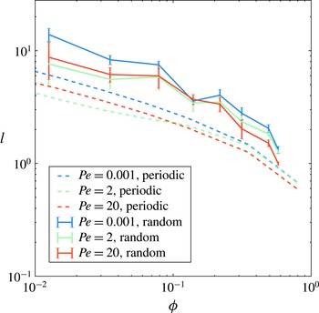
) is within 2 % of the asymptote. This slip distance is plotted in figure 11 for varying area fractions and values of the Péclet number. For any Péclet number, the slip distance ultimately decreases with increasing area fraction, as the wakes are shared across all disks and a majority of the surface becomes reactive. In the dilute limit of disks, each disk is effectively isolated from the influence of neighbouring disks and its wake extends long distances into the bulk from the surface (figure 5
b). Nevertheless, one sees that the slip distance hits a plateau in the dilute limit, which reduces in value for increasing Péclet number. This is consistent with the flattening of the wake over the surface as the Péclet number increases, i.e. the depletion region is compressed.
The slip length,
 $l$
, at which there is only 2 % variation from the value of the asymptote, is graphed for varying area fraction and Péclet number. Here,
 ${\it\kappa}=300$
.

Beyond the slip distance, the concentration field is approximately the same as the asymptotic form (3.2d
), and this information can be used as a matching boundary condition implemented at the slip distance, to replace the details of the heterogeneous surface. The effective reaction rate associated with the boundary condition is
 ${\it\kappa}_{eff}=Sh_{p}({\it\kappa},\mathit{Pe},{\it\phi}){\it\phi}$
. At large area fractions,
 $Sh_{p}\approx {\it\kappa}$
for all Péclet numbers, as the majority of the surface is reactive. In the dilute limit, the effect of the flow is felt on the Sherwood number, especially at large Péclet number (figure 9
a). In particular, the Sherwood number is always bound from above by the conventional approximation to the flux given by the value of the Damköhler number (Herskowitz et al.
Reference Herskowitz, Carbonell and Smith1979),
 $Sh_{p}\approx {\it\kappa}$
. The error in the simple approximation is then given by the quantity
 $$\begin{eqnarray}{\it\eta}=\frac{{\it\kappa}}{Sh_{p}({\it\kappa},\mathit{Pe},{\it\phi})}-1.\end{eqnarray}$$
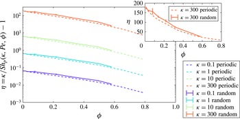
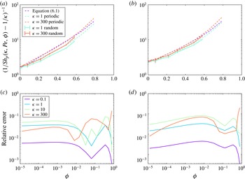
In figure 12 we map this error versus the area fraction of disks for various values of the Damköhler number. In the dilute limit,
 $Sh_{p}\approx Sh_{u}$
, which is given by the approximation (2.11), so the error is never close to zero except in the kinetically limited regime (the bottom curve in figure 12) or at large area fraction. Since we consider only circular non-overlapping disks in our simulations, we are able to simulate up to
 ${\it\phi}=0.78$
. It can be seen that even at such large area fractions, for a diffusion-limited regime the error in the simple approximation
 $Sh_{p}\approx {\it\kappa}$
is almost a factor of 10 (topmost curve). This indicates that the Sherwood number is nearly independent of the area fraction when
 ${\it\phi}\leqslant 10^{-2}$
. By analysing the difference
 $Sh_{p}-Sh_{u}$
in the ensuing section, we are able to conclude that
 $Sh_{p}$
can be replaced with
 $Sh_{u}$
with at most 3 % error for area fractions of up to
 $10^{-2}$
. However, to obtain
 $Sh_{p}$
to a good degree of approximation, without solving (3.8) and for non-dilute regimes, we must use other approximations, as detailed in § 5.
From (3.19),
 ${\it\eta}={\it\kappa}/Sh_{p}({\it\kappa},\mathit{Pe},{\it\phi})-1$
is plotted against the area fraction
 ${\it\phi}$
for Péclet number
 $\mathit{Pe}=2$
and varying Damköhler number in both the periodic and the random cases. Inset: a normal scale plot of
 ${\it\eta}$
for the case of
 ${\it\kappa}=300$
to indicate the size of the error bars at each data point in the random case.

4. Random distribution of disks in a periodic system
As (3.2d
) is independent of the shape and sizes of reacting regions, it can be used to determine the concentration field and the Sherwood number in the case of random disordered periodic media. Such media are modelled as a periodic distribution of random disordered disks in each box
 $\mathscr{B}_{n}$
, as seen in figure 13. As mentioned before, we refer to this case as simply ‘random’. We perform simulations of 10 disks of unit radius distributed randomly in a periodic domain, each with
 $O(1000)$
elements. For each disk area fraction, we simulate 10 such distributions and gather the statistics for the Sherwood number, the slip length and other relevant quantities.
Disordered periodic distribution of reacting disks in the domain.

4.1. Effective reaction rate and slip distance
As in § 3.4, we recall that the slip length is the wall-normal distance into the bulk at which the concentration field uniformly exhibits the far-field behaviour (3.2d ). We arbitrarily chose this to be the distance at which the concentration field is within 2 % of the far-field value over all disks. To compare the slip distances in the random and periodic cases, we plot both quantities in figure 11 for a range of Péclet numbers. While the slip distance for the random case is consistently larger than that for the periodic case for any given Péclet number, it still scales with the disk radius for all Péclet numbers. This may be explained by the observation that a smaller slip length should result from the more efficient wake sharing (hence, a flatter depletion region), as in the case of a regular periodic distribution.
One can expect the wake-sharing effect to be weaker due to disorder, so the Sherwood number in the random case will be smaller than that in the simply periodic case of § 3.3 at any disk area fraction. To confirm this, in figure 12 we overlaid the curves for the periodic case with the Sherwood number for the random case. It is important to note that as the disks are non-overlapping, we reach a maximum disk area fraction corresponding to the maximum packing fraction in a plane. However, in the limit of large area fraction of reacting disks, even before the maximum packing fraction is reached, the distribution is no longer truly disordered, and thus the Sherwood number in the random case approaches the value of its periodic counterpart. Consequently, the error in the simple approximation, given by (3.19), is almost the same for the random and the periodic cases for large
 ${\it\phi}$
, as seen in the inset in figure 12. In the dilute limit for random disks, the majority of the disks are effectively isolated from each other with high probability. Then, the Sherwood number is again close in value to its periodic counterpart. This observation is supported by the results of Juhasz & Deen (Reference Juhasz and Deen1993), who measured the limiting current generated at a rotating electrode patterned with reactive sites. It was found that the limiting current in a laminar flow (at
 $\mathit{Pe}\gg 1$
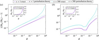
) depends subtly on the electrode distribution for small pattern coverages. Thus, intriguingly but not surprisingly, the flux in the two cases is not very different at all disk area fractions (
 ${<}$
20 % relative error with respect to the Sherwood number in the periodic case). It should be noted that the standard deviation for each data point looks deceptively small on the log-scale plots but its size is clearly seen in the inset.
5. Effect of disk area fraction – dilute systems
Consider a single circular unit disk
 $\mathscr{P}$
in the unbounded domain case and a corresponding periodic problem with disk
 $\mathscr{P}_{0}$
coinciding with
 $\mathscr{P}$
. As observed from the isotherms in figures 5(a) and 10(a), the surface concentration field in the periodic case is different from that in the unbounded domain case only in the far field and close to the periodic boundary of
 $\mathscr{B}_{0}$
. To the first order in disk area fraction, this difference between the two fields can be directly attributed to the disparity between the two Green’s functions. Specifically, the periodic Green’s function can be constructed as a summation of the isolated ones with source singularities at lattice points. To guarantee convergence of the summation, in each summand with corresponding source at
 $\boldsymbol{r}_{\boldsymbol{n}}\in \mathscr{B}_{\boldsymbol{n}}$
, we subtract a solution corresponding to a uniform sink of strength
 $1/B_{0}$
over
 $\mathscr{B}_{\boldsymbol{n}}$
. Superposition allows us to sum the sink solutions for individual small tiles
 $\mathscr{B}_{\boldsymbol{n}}$
to a uniform sink solution for a large tile defined by the finite union
 $\mathscr{B}=\cup \mathscr{B}_{\boldsymbol{n}}$
. The isolated Green’s function decays as
 $1/x_{1}$
in the shear direction, so most of the difference
 $G_{p}-G_{u}$
is a summation of the four nearest neighbouring Green’s functions and corresponding sink solutions. As the effect of each neighbouring Green’s function is
 $1/\boldsymbol{L}_{1}$
, the difference
 $G_{p-u}(\boldsymbol{y}\mid \boldsymbol{x}_{b};Pe)=(G_{p}(\boldsymbol{y}\mid \boldsymbol{x}_{b};Pe)-G_{u}(\boldsymbol{y}\mid \boldsymbol{x}_{b};Pe))$
is
 $O({\it\phi}^{1/2})$
to leading order for small
 ${\it\phi}$
. Consequently, the difference between the two Sherwood numbers is also
 $O({\it\phi}^{1/2})$
in the dilute limit.
5.1. Formal expansion
To formalize this, we expand the concentration in the periodic case to the first order in
 ${\it\phi}$
as
 $$\begin{eqnarray}C_{p}=C_{u}+C^{(1)}{\it\phi}^{1/2}+\cdots \,,\end{eqnarray}$$
with the aim of obtaining the first-order correction to
 $Sh_{u}$
. We rewrite (2.4) as
 $$\begin{eqnarray}C_{p}(\boldsymbol{x})=1-{\it\kappa}\int _{\mathscr{P}}G_{u}(\boldsymbol{y}_{b}\mid \boldsymbol{x};Pe)C_{p}(\boldsymbol{y}_{b})\,\text{d}A(\boldsymbol{y}_{b})-{\it\kappa}\int _{\mathscr{P}}G_{p-u}(\boldsymbol{y}_{b}\mid \boldsymbol{x};Pe)C_{p}(\boldsymbol{y}_{b})\,\text{d}A(\boldsymbol{y}_{b}).\end{eqnarray}$$
On substituting the expansion for
 $C_{p}$
and subtracting (3.8) from the above, we obtain the first-order term in the expansion of
 $C_{p}$
,
 $$\begin{eqnarray}C^{(1)}(\boldsymbol{x})=-{\it\kappa}\int _{\mathscr{ P}}G_{u}(\boldsymbol{y}_{b}\mid \boldsymbol{x};Pe)C^{(1)}(\boldsymbol{y}_{b})\,\text{d}A(\boldsymbol{y}_{b})-{\it\kappa}{\it\phi}^{-1/2}\int _{\mathscr{P}}G_{p-u}(\boldsymbol{y}_{b}\mid \boldsymbol{x};Pe)C_{u}(\boldsymbol{y}_{b})\,\text{d}A(\boldsymbol{y}_{b}).\end{eqnarray}$$
Expanding
 $G_{p-u}$
as a multipole about the origin as reference and retaining the first-order term (which is
 $O({\it\phi}^{1/2})$
) yields
 $$\begin{eqnarray}C^{(1)}(\boldsymbol{x})=-{\it\kappa}\int _{\mathscr{ P}}G_{u}(\boldsymbol{y}_{b}\mid \boldsymbol{x};Pe)C^{(1)}(\boldsymbol{y}_{b})\,\text{d}A(\boldsymbol{y}_{b})-{\it\phi}^{-1/2}|\mathscr{P}|G_{p-u}(\mathbf{0}\mid \boldsymbol{x};Pe)Sh_{u}({\it\kappa},Pe).\end{eqnarray}$$
Solving (5.4) for
 $C^{(1)}$
, we now evaluate the correction term
 $$\begin{eqnarray}(Sh_{p}-Sh_{u})/Sh_{u}\approx {\it\kappa}{\it\phi}^{1/2}\int _{\mathscr{P}}C^{(1)}(\boldsymbol{x}_{b})\,\text{d}A(\boldsymbol{x}_{b})/(|\mathscr{P}|Sh_{u}),\end{eqnarray}$$
and compare with the exact value obtained from solving (2.4) and (3.8).
In figure 14 it is immediately seen that the exact correction is matched by the prediction of (5.5) at area fractions up to
 $O(10^{-1})$
. Moreover, both the exact values and perturbation theory predict that the corrections grow as
 ${\it\phi}^{1/2}$
at all Péclet numbers in the dilute limit of the area fraction. Additionally, to obtain
 $Sh_{p}$
, the correction to
 $Sh_{u}$
is, for all practical purposes, negligible (
 ${<}$
3 % of
 $Sh_{u}$
) for area fractions up to
 $O(10^{-2})$
. We recall from § 3.3 that there exists a corresponding area fraction for which
 $\mathit{Pe}=10$
is the cutoff Péclet number. Then, for smaller area fractions,
 $Sh_{p}<Sh_{u}$
, and at larger area fractions,
 $Sh_{p}>Sh_{u}$
. Subsequently, this introduces a sign change in the value of
 $Sh_{p}/Sh_{u}-1$
, which is visually seen as the kink in the logarithmic plot. The sign change is also visible from the slight dip below 0 of the curve in the inset of figure 14(b). This perturbation approach can be readily extended to calculate higher-order corrections in
 ${\it\phi}$
. However, we expect that it will be difficult to match the details of the exact curve at large area fractions (
 ${\it\phi}\sim O(1)$
) with only a couple of terms. This is seen in the large deviation of the predictions of (5.5) from the exact correction curve for
 ${\it\kappa}=300$
in figure 14(b). Perturbation theory by itself also does not yield an easily computable correction, which behoves us to use another approximation theory. This approximation makes use of the assumption that most of the information on the field is contained in the monopole of the multipole expansion.
The absolute value of the correction to
 $Sh_{u}$
to obtain
 $Sh_{p}$
for both perturbation theory (5.5) and exact values (boundary integral solution) at (a)
 $\mathit{Pe}=0.001$
and (b)
 $\mathit{Pe}=10$
. Certainly, at vanishing
 ${\it\phi}$
, the correction is
 ${\sim}O({\it\phi}^{1/2})$
. The inset shows that at
 $\mathit{Pe}=10$
,
 $Sh_{p}<Sh_{u}$
as
 ${\it\phi}\rightarrow 0$
and
 $Sh_{p}>Sh_{u}$
at large
 ${\it\phi}$
, i.e.
 $Sh_{p}/Sh_{u}-1$
changes sign at an intermediate
 ${\it\phi}$
. This sign change occurs at very small
 ${\it\phi}$
when
 $\mathit{Pe}\ll 1$
.

6. Method of resistances and developing correlations
As in § 2.2, we propose a method of additive resistances argument to calculate an approximate expression for the Sherwood number in the periodic case. The hypothesis is that the resistance
 $1/Sh_{p}({\it\kappa},\mathit{Pe},{\it\phi})$
is the sum of two resistances,
 $1/Sh_{p}(\infty ,\mathit{Pe},{\it\phi})$
and
 $1/{\it\kappa}$
, corresponding to transport from the far field to the microscale and then from the microscale to the disk, thus
 $$\begin{eqnarray}\frac{1}{Sh_{p}({\it\kappa},\mathit{Pe},{\it\phi})}\approx \frac{1}{Sh_{p}(\infty ,\mathit{Pe},{\it\phi})}+\frac{1}{{\it\kappa}}.\end{eqnarray}$$
To confirm the hypothesis, we simply need to show numerically that the quantity
 ${\it\zeta}=(1/Sh_{p}({\it\kappa},\mathit{Pe},{\it\phi})-1/{\it\kappa})^{-1}$
is nearly independent of
 ${\it\kappa}$
. We plot this quantity against the area fraction for multiple values of the Damköhler number in figure 15. As is evident from the figure,
 ${\it\zeta}$
for both the periodic and the random cases seems to depend on
 ${\it\kappa}$
remarkably weakly as the value of
 ${\it\kappa}$
is varied over orders of magnitude, thus proving our hypothesis true. Indeed, at vanishing area fraction, all of the curves approach one value where
 ${\it\zeta}=Sh_{u}(\infty ,Pe)$
. As a corollary, one can show that the cutoff Péclet number of § 3.3, where
 $Sh_{u}-Sh_{p}$
changes sign, is nearly independent of
 ${\it\kappa}$
for a given area fraction. This follows from the observation that
 $Sh_{u}-Sh_{p}$
changes sign when
 $1/Sh_{u}({\it\kappa},Pe)-1/Sh_{p}({\it\kappa},\mathit{Pe},{\it\phi})\approx 1/Sh_{u}(\infty ,Pe)-1/Sh_{p}(\infty ,\mathit{Pe},{\it\phi})$
changes sign.
Plot of
 ${\it\zeta}=(1/Sh_{p}({\it\kappa},\mathit{Pe},{\it\phi})-1/{\it\kappa})^{-1}$
versus
 ${\it\phi}$
for a wide range of the Damköhler number at (a)
 $\mathit{Pe}=2$
and (b)
 $\mathit{Pe}=20$
. The curves for both the random and the periodic cases nearly collapse to a single curve. This provides numerical evidence for the method of resistances argument to be true, and also shows the utility of the approximation (6.2). The relative error (in absolute value) in using (6.2) for predicting the Sherwood number for periodic domains is plotted in (c) for
 $\mathit{Pe}=2$
and (d) for
 $\mathit{Pe}=20$
.

Figure 15 suggests that a single approximation can be used to predict the Sherwood number for both the periodic and the random distributions. The method of resistances provides a way to calculate the Sherwood number at arbitrary
 ${\it\kappa}$
once we approximate
 $Sh_{p}(\infty ,\mathit{Pe},{\it\phi})$
. The quality of the approximation to
 $Sh_{p}(\infty ,\mathit{Pe},{\it\phi})$
affects the accuracy of the overall approximation. We now develop an approximation to
 $Sh_{p}(\infty ,\mathit{Pe},{\it\phi})$
, just as we did for
 $Sh_{u}(\infty ,Pe)$
in § 2.2. First, we define a variable
 $t:\, [0,1)\rightarrow [0,\infty ),$
where
 $t={\it\phi}/(1-{\it\phi})$
for
 ${\it\phi}\in \, [0,1)\,$
. Thus,
 $t$
is the ratio of the reacting and non-reacting surface areas. We observe that
 $Sh_{p}(\infty ,\mathit{Pe},t)\rightarrow Sh_{u}(\infty ,Pe)$
as
 $t\rightarrow 0$
. Additionally,
 $\lim _{t\rightarrow \infty }Sh_{p}(\infty ,\mathit{Pe},t)=\infty$
. Then, one can assume that
 $Sh_{p}(\infty ,Pe,t)={\it\alpha}t^{m}+\cdots \,$
to leading order in
 $t$
. The scaling exponent
 $m$
is extracted from figure 15 by plotting all data on a log-scale graph with
 $t$
on the
 $x$
-axis. It is observed that
 $m=1$
. Then, we can write the approximation
 $Sh_{p}(\infty ,\mathit{Pe},t)=[(Sh_{u}(\infty ,Pe))^{s}+({\it\alpha}t)^{s}]^{1/s}$
(Churchill & Usagi Reference Churchill and Usagi1972). Here,
 $A$
and
 $s$
are fitting parameters so that
 $Sh_{p}(\infty ,\mathit{Pe},t)$
matches the curves in figure 15. It is reasonable to expect that the best fits for
 ${\it\alpha}$
and
 $s$
will depend on the value of the Péclet number. Fortunately, we find that fitting
 ${\it\alpha}=9,s=3/2$
yields an expression that predicts the periodic Sherwood number within 10 % error across a wide range of values of the Péclet number, as seen in figure 15. This expression is made explicit by substituting
 $Sh_{u}(\infty ,Pe)$
from (2.10), and we obtain
 $$\begin{eqnarray}Sh_{p}(\infty ,\mathit{Pe},{\it\phi})=\left[\left(\frac{4}{{\rm\pi}}\right)^{3/2}(1+0.3959\mathit{Pe}^{1/2})+\left(\frac{9{\it\phi}}{1-{\it\phi}}\right)^{3/2}\right]^{2/3}.\end{eqnarray}$$
This approximation generally overestimates the Sherwood number in the periodic case. As the Sherwood number in the random case is always smaller than that in the periodic case, we should choose different values for
 ${\it\alpha}$
and
 $s$
to fit the random case. The various correlations of this section and § 2.2 are summarized in table 1. It should be noted that the correlation (6.2) suggests that in the limit as
 ${\it\kappa}\rightarrow \infty$
and
 $(1-{\it\phi})\ll 1$
, the flux is controlled by the (small) region of non-reactive surface, such that
 $Sh_{p}\propto 1/(1-{\it\phi})$
. This is certainly worthy of further examination outside the scope of this work.

7. Conclusions
We have demonstrated through accurate numerical simulations that the problem of mass transport to a heterogeneous surface with first-order reactive patches can be modelled as a problem of mass transfer to a surface with a homogeneous effective first-order reaction rate
 ${\it\kappa}_{eff}$
(cf. (3.14), § 3.2). This effective rate is related to the Sherwood number on the microscale, which in turn is related to the local reaction and shear rates. The influence of the configuration of the reactive patches (or disks) on
 ${\it\kappa}_{eff}$
is captured by a single quantity, the disk area fraction
 ${\it\phi}$
, as the Sherwood number depends strongly on the area fraction and weakly on the disorder (figures 12 and 15). The slip distance at which the effect of heterogeneity is screened by the flow scales with the length scale of the individual disks (figure 11).
The effect of the local reaction rate, dominant over the reaction length scale, can be separated from the effects of the far field, which lays the foundation for the method of additive resistances in §§ 2.2 and 6. Then, to gain a qualitative understanding of the physics, one only needs to analyse the effect of the far field and study the problem of transport to purely adsorbing disks (
 ${\it\kappa}\rightarrow \infty$
). In principle, this can be accomplished by studying the two asymptotic limits of
 $\mathit{Pe}\ll 1$
and
 $\mathit{Pe}\gg 1$
. In the limit of large Péclet number, we have extensive downstream wake sharing when multiple reactive disks are present, as the disks are insensitive to transport in the vorticity direction. The effect of efficient wake sharing is a net reduction in the Sherwood number (§ 2.4). When the Péclet number is small, the neighbouring disks in all directions have an effect on the flux through a given disk. In particular, the neighbours in the vorticity direction augment the gradients in that direction, causing a net increase in the Sherwood number. Consequently, at an intermediate Péclet number, the Sherwood numbers for the periodic and the unbounded cases are exactly equal. This cutoff Péclet number is almost independent of the value of
 ${\it\kappa}$
(figure 9
a), and is thus only a function of the area fraction. In the unbounded case, we are able to construct expressions for the Sherwood number to the leading order in
 $Pe$
for the two limiting regimes and bridge them to obtain an approximate expression for
 $Sh_{u}$
in
 $({\it\kappa},Pe)$
.
To obtain similar approximations for
 $Sh_{p}$
in the periodic and random cases, we first quantify the effect of disk area fraction in the dilute regime (5) and attribute it to the long-range nature of the monopole (Green’s function) associated with the integral equation in the unbounded domain case. To explain the effect of large area fraction, we use the method of resistances (6.1) along with an approximation for the Sherwood number in the diffusion-limited regime (6.2). The power and utility of our theory can be demonstrated by considering the following example.
7.1. Example: isolated circular domain composed of circular subdomains
Assume an isolated circular domain composed of randomly placed smaller circular subdomains, where the random subdomains have a local Damköhler number
 ${\it\kappa}=1$
and the flow over the subdomains has a Péclet number
 $\mathit{Pe}=1$
. The radius of the large circular domain is 50 while the subdomains are disks of unit radius (note that
 $50\gg l^{\ast }$
for all conditions). We can use three approximations for the dimensionless effective reaction rate constant (
 ${\it\kappa}_{eff}$
) for the disordered surface: the simple approximation (
 ${\it\kappa}_{eff_{1}}={\it\phi}{\it\kappa}$
), the ‘non-interacting’ approximation (
 ${\it\kappa}_{eff_{2}}={\it\phi}Sh_{u}$
) and the ‘correct’ result (
 ${\it\kappa}_{eff_{3}}={\it\phi}Sh_{p}$
). We do this for
 ${\it\phi}=0.126,0.35$
and
 $0.5$
. We estimate the Sherwood number for the entire domain of radius
 $r$
using the expression (2.11) (see table 1) and ‘outer’ Péclet and Damköhler numbers given by
 $\mathit{Pe}_{o}=r^{2}Pe,{\it\kappa}_{o}={\it\kappa}r$
. The ‘outer’ parameters are obtained by showing that the governing equations for a disk of radius
 $r$
are equivalent to those for a unit disk under a change of length scale (
 $X_{i}=rx_{i}$
). Three Sherwood numbers
 $Sh_{u_{1}},Sh_{u_{2}},Sh_{u_{3}}$
are calculated using
 $Sh_{u_{i}}=Sh_{u}({\it\kappa}_{o_{i}},\mathit{Pe}_{o})=Sh_{u}(50{\it\kappa}_{eff_{i}},50^{2}Pe)$
. Table 2 shows the values of the three Sherwood numbers. Table 3 is the same table but corresponding to a local Damköhler number of
 ${\it\kappa}=300$
. We see that even when the subdomains are in the diffusion-limited regime (
 ${\it\kappa}\gg 1$
), the outer circular domain can be in the intermediate regime of
 ${\it\kappa}_{o}\sim O(10)$
.
Values for the outer Damköhler number using
 ${\it\kappa}_{o}=50{\it\kappa}_{eff}$
and the three approximations
 ${\it\kappa}_{eff_{1}}={\it\phi}{\it\kappa}$
,
 ${\it\kappa}_{eff_{2}}={\it\phi}Sh_{u}({\it\kappa},Pe)$
,
 ${\it\kappa}_{eff_{3}}={\it\phi}Sh_{p}({\it\kappa},\mathit{Pe},{\it\phi})$
and corresponding Sherwood numbers,
 $Sh_{ui}=Sh_{u}(50{\it\kappa}_{eff_{i}},50^{2}Pe)$
, for
 $\mathit{Pe}=1,{\it\kappa}=1$
at the subdomain scale and
 ${\it\phi}=0.126,0.35,0.5$
. The data are rounded up to 3 significant digits.

Values for the outer Damköhler number using
 ${\it\kappa}_{o}=50{\it\kappa}_{eff}$
and the three approximations
 ${\it\kappa}_{eff_{1}}={\it\phi}{\it\kappa}$
,
 ${\it\kappa}_{eff_{2}}={\it\phi}Sh_{u}({\it\kappa},Pe)$
,
 ${\it\kappa}_{eff_{3}}={\it\phi}Sh_{p}({\it\kappa},\mathit{Pe},{\it\phi})$
and corresponding Sherwood numbers,
 $Sh_{ui}=Sh_{u}(50{\it\kappa}_{eff_{i}},50^{2}Pe)$
, for
 $\mathit{Pe}=1,{\it\kappa}=300$
at the subdomain scale and
 ${\it\phi}=0.126,0.35,0.5$
. The data are rounded up to 3 significant digits.

It should be noted that the three approximations can give very different values for
 ${\it\kappa}_{eff}$
, depending on the local Damköhler number. Thus, the Sherwood number predicted for each approximation is also different. We notice that the simple approximation always overestimates (sometimes severely, depending on the value of the local
 ${\it\kappa}$
) the outer Damköhler number. Since
 $Sh_{u}$
is monotonic in
 ${\it\kappa}$
, the simple approximation overestimates the Sherwood number as well. The outer Damköhler number in the non-interacting case and the corresponding Sherwood number have the lowest values of all. Physically, modelling each subdomain as non-interacting generally underpredicts the Sherwood number for the domain. Once we take into account the interactions between the subdomains, we obtain the ‘correct’ values for the Sherwood number and the outer Damköhler number.
To conclude, we have a mathematical theory and a computational method that allow calculation of the effective transport coefficients in the problem of mass transfer to first-order reactive patches on a flat surface submerged in a linear shear flow. As the theory and computational algorithm are valid for any shape and configuration of reactive domains, we plan to explore the regime of
 ${\it\phi}\approx 1$
as the subject of a second paper. The method of resistances suggests that we only need to investigate the diffusion-limited regime of the Damköhler number.
Acknowledgements
The authors would like to acknowledge Professor A. Acrivos for extensive discussions regarding the history of this problem in the context of reaction engineering and many valuable inputs regarding the method of resistances. The authors are grateful for the funding support provided by the Stanford Graduate Engineering Fellowship, and NSF-MRI2 award 0960306 for providing computing resources that contributed to the research.
Appendix A
A.1. The unbounded Green’s function
The Green’s function
 $G_{u}$
is related to
 $G_{\boldsymbol{k}}^{u}$
, its Fourier transform about the point
 $\boldsymbol{y}_{s}$
, by the following relations:
 $$\begin{eqnarray}\displaystyle & \displaystyle G_{u}(\boldsymbol{x}\mid \boldsymbol{y};Pe)=\int _{-\infty }^{\infty }\int _{-\infty }^{\infty }G_{\boldsymbol{k}}^{u}\text{e}^{-\text{i}\boldsymbol{k}\boldsymbol{\cdot }(\boldsymbol{x}_{s}-\boldsymbol{y}_{s})}\,\text{d}k_{1}\,\text{d}k_{2}, & \displaystyle\end{eqnarray}$$
 $$\begin{eqnarray}\displaystyle & \displaystyle G_{\boldsymbol{k}}^{u}=\frac{1}{(2{\rm\pi})^{2}}\int _{-\infty }^{\infty }\int _{-\infty }^{\infty }G_{u}(\boldsymbol{x}\mid \boldsymbol{y};Pe)\text{e}^{\text{i}\boldsymbol{k}\boldsymbol{\cdot }(\boldsymbol{x}_{s}-\boldsymbol{y}_{s})}\,\text{d}x_{1}\,\text{d}x_{2}. & \displaystyle\end{eqnarray}$$
 $\boldsymbol{y}_{s}$
, to obtain (with
 $k^{2}=k_{1}^{2}+k_{2}^{2}$
)
 $$\begin{eqnarray}\displaystyle & \displaystyle \frac{\text{d}^{2}G_{\boldsymbol{ k}}^{u}}{\text{d}x_{3}^{2}}-(k^{2}+\text{i}\,\mathit{Pe}\,k_{1}x_{3})G_{\boldsymbol{k}}^{u}=-\frac{1}{(2{\rm\pi})^{2}}{\it\delta}(x_{3}-y_{3}), & \displaystyle\end{eqnarray}$$
 $$\begin{eqnarray}\displaystyle & \displaystyle \frac{\text{d}G_{\boldsymbol{k}}^{u}}{\text{d}x_{3}}=0\quad \text{at }x_{3}=0, & \displaystyle\end{eqnarray}$$
 $$\begin{eqnarray}\displaystyle & \displaystyle G_{\boldsymbol{k}}^{u}\rightarrow 0,\quad \text{as }x_{3}\rightarrow \infty . & \displaystyle\end{eqnarray}$$
 $x_{3}$
to
 $s$
, where
 $$\begin{eqnarray}s(x_{3})=\frac{k^{2}+\text{i}\,\mathit{Pe}\,k_{1}x_{3}}{(\text{i}\,\mathit{Pe}\,k_{1})^{2/3}}.\end{eqnarray}$$
With this change of variables, we obtain the equations in Fourier space,
 $$\begin{eqnarray}\frac{\text{d}^{2}G_{\boldsymbol{k}}^{u}}{\text{d}s^{2}}-sG_{\boldsymbol{k}}^{u}=-\frac{1}{(2{\rm\pi})^{2}(\text{i}\,\mathit{Pe}\,k_{1})^{2/3}}{\it\delta}(x_{3}-y_{3}).\end{eqnarray}$$
It is easily seen that
 $G_{\boldsymbol{k}}^{u}$
is a linear combination of Airy functions of the first and second kind in the two regions
 $0\leqslant x_{3}\leqslant y_{3}$
and
 $\infty >x_{3}\geqslant y_{3}$
:
 $$\begin{eqnarray}G_{\boldsymbol{k}}^{u}=\left\{\begin{array}{@{}ll@{}}A_{1}\text{Ai}(s)+B_{1}\text{Bi}(s),\quad & 0\leqslant x_{3}\leqslant y_{3},\\ A_{2}\text{Ai}(s)+B_{2}\text{Bi}(s),\quad & \infty >x_{3}\geqslant y_{3}.\end{array}\right.\end{eqnarray}$$
The above solution form should be continuous at
 $x_{3}=y_{3}$
while also having a jump in its derivative at
 $x_{3}=y_{3}$
,
 $$\begin{eqnarray}\displaystyle \displaystyle G_{\boldsymbol{k}}^{u}|_{x_{3}\rightarrow y_{3}^{+}} & = & \displaystyle G_{\boldsymbol{k}}^{u}|_{x_{3}\rightarrow y_{3}^{-}},\end{eqnarray}$$
 $$\begin{eqnarray}\displaystyle \displaystyle \left.\frac{\text{d}G_{\boldsymbol{k}}^{u}}{\text{d}x_{3}}\right|_{x_{3}\rightarrow y_{3}^{+}} & = & \displaystyle \left.\frac{\text{d}G_{\boldsymbol{k}}^{u}}{\text{d}x_{3}}\right|_{x_{3}\rightarrow y_{3}^{-}}-\frac{1}{(2{\rm\pi})^{2}}.\end{eqnarray}$$
Coupled with the boundary conditions (A 2b
,
c
), continuity conditions (A 5a
,
b
) are sufficient to solve for the constants
 $A_{1},A_{2},B_{1}$
and
 $B_{2}$
and yield the final solution form
 $$\begin{eqnarray}G_{\boldsymbol{k}}^{u}=\left\{\begin{array}{@{}ll@{}}\displaystyle \frac{-{\rm\pi}\text{Ai}(s_{y_{3}})(\text{Ai}(s)\text{Bi}^{\prime }(s_{0})-\text{Bi}(s)\text{Ai}^{\prime }(s_{0}))}{(2{\rm\pi})^{2}\text{Ai}^{\prime }(s_{0})(\text{i}\,\mathit{Pe}\,k_{1})^{1/3}},\quad & 0\leqslant x_{3}\leqslant y_{3},\\ \displaystyle \frac{-{\rm\pi}\text{Ai}(s)(\text{Ai}(s_{y_{3}})\text{Bi}^{\prime }(s_{0})-\text{Bi}(s_{y_{3}})\text{Ai}^{\prime }(s_{0}))}{(2{\rm\pi})^{2}\text{Ai}^{\prime }(s_{0})(\text{i}\,\mathit{Pe}\,k_{1})^{1/3}},\quad & \infty >x_{3}\geqslant y_{3},\end{array}\right.\end{eqnarray}$$
where
 $s_{y_{3}}=s(y_{3})$
and
 $s_{0}=s(0)$
. Let us define the Airy kernel
 $$\begin{eqnarray}K_{A}(x,y)=\text{Ai}(x)\text{Bi}^{\prime }(y)-\text{Ai}^{\prime }(y)\text{Bi}(x).\end{eqnarray}$$
On inverting the transform, we obtain the following form for the Green’s function for the isolated disks:
 $$\begin{eqnarray}\displaystyle G_{u}(\boldsymbol{x}\mid \boldsymbol{y};Pe)=\left\{\begin{array}{@{}ll@{}}\displaystyle \frac{-1}{(2{\rm\pi})^{2}}\int _{-\infty }^{\infty }\int _{-\infty }^{\infty }\frac{{\rm\pi}\text{Ai}(s_{y_{3}})K_{A}(s,s_{0})}{\text{Ai}^{\prime }(s_{0})(\text{i}\,\mathit{Pe}\,k_{1})^{1/3}}\text{e}^{-\text{i}\boldsymbol{k}\boldsymbol{\cdot }(\boldsymbol{x}_{s}-\boldsymbol{y}_{s})}\,\text{d}k_{1}\,\text{d}k_{2},\quad & 0\leqslant z\leqslant y_{3},\\ \displaystyle \frac{-1}{(2{\rm\pi})^{2}}\int _{-\infty }^{\infty }\int _{-\infty }^{\infty }\frac{{\rm\pi}\text{Ai}(s)K_{A}(s_{y_{3}},s_{0})}{\text{Ai}^{\prime }(s_{0})(\text{i}\,\mathit{Pe}\,k_{1})^{1/3}}\text{e}^{-\text{i}\boldsymbol{k}\boldsymbol{\cdot }(\boldsymbol{x}_{s}-\boldsymbol{y}_{s})}\,\text{d}k_{1}\,\text{d}k_{2},\quad & \infty >z\geqslant y_{3}.\end{array}\right. & & \displaystyle \nonumber\\ \displaystyle & & \displaystyle\end{eqnarray}$$
The Green’s function of (2.3) is recovered from the above equation by setting
 $y_{3}=0$
and using the identity that for any
 $x$
,
 $\text{Ai}(x)\text{Bi}^{\prime }(x)-\text{Bi}(x)\text{Ai}^{\prime }(x)=1/{\rm\pi}$
. In particular, Stone (Reference Stone1989) obtained a Green’s function, which we derive from (2.3) by setting
 $x_{3}=0$
,
 $$\begin{eqnarray}\bar{G}_{u}(\boldsymbol{x}_{s}\mid \boldsymbol{y}_{s};Pe)=\frac{1}{(2{\rm\pi})^{2}}\int _{-\infty }^{\infty }\int _{-\infty }^{\infty }\frac{-\text{Ai}(s_{0})}{\text{Ai}^{\prime }(s_{0})(\text{i}\,\mathit{Pe}\,k_{1})^{1/3}}\text{e}^{-\text{i}\boldsymbol{k}\boldsymbol{\cdot }(\boldsymbol{x}_{s}-\boldsymbol{y}_{s})}\,\text{d}k_{1}\,\text{d}k_{2}.\end{eqnarray}$$
A.2. Computing the periodic Green’s function
As the Fourier coefficients
 $G_{\boldsymbol{k}}^{p}$
decay slowly (
 ${\sim}1/(B_{0}k)$
) when
 $k\rightarrow \infty$
, we are left with a slowly converging series in trigonometric functions in (3.6). We adopt the same strategy as in the unbounded case by writing
 $G_{\boldsymbol{k}}^{p}=(G_{\boldsymbol{k}}^{p}-1/(B_{0}k))+1/(B_{0}k)$
. The difference in the brackets converges quickly in the Fourier domain. On the other hand, the Fourier series
 ${\it\sigma}_{1/2}(\boldsymbol{r})=\sum 1/(B_{0}k)\exp (\text{i}\boldsymbol{k}\boldsymbol{\cdot }\boldsymbol{r})$
corresponding to the second term is evaluated efficiently using Evald’s summation technique, as discussed by Hasimoto (Reference Hasimoto1959) and explained in brief in § A.7:
 $$\begin{eqnarray}{\it\sigma}_{1/2}(\boldsymbol{r})=\mathop{\sum }_{\boldsymbol{n}}\frac{\text{erfc}(\sqrt{{\rm\pi}/{\it\alpha}}\Vert \boldsymbol{r}-\boldsymbol{y}_{\boldsymbol{n}}\Vert )}{2{\rm\pi}\Vert \boldsymbol{r}-\boldsymbol{y}_{\boldsymbol{n}}\Vert }-\frac{1}{{\rm\pi}B_{0}}+\mathop{\sum }_{k\neq 0}\frac{\text{e}^{-\text{i}\boldsymbol{k}\boldsymbol{\cdot }\boldsymbol{r}}}{B_{0}k}\text{erfc}(\sqrt{{\it\alpha}k^{2}/4{\rm\pi}}).\end{eqnarray}$$
The complementary error function is denoted by
 $\text{erfc}$
. It should be noted that in the case of
 $k_{1}=0$
, for the sake of computational convenience, the Fourier coefficient
 $G_{\boldsymbol{k}}^{p}$
can be derived directly from (A 19a
–
c
) and (A 21a
,
b
):
 $$\begin{eqnarray}G_{(0,k_{2})}^{\mathit{p}}=\left\{\begin{array}{@{}ll@{}}\displaystyle \frac{1}{2|k_{2}|B_{0}}\text{e}^{-|k_{2}|y_{3}}(\text{e}^{-k_{2}x_{3}}+\text{e}^{k_{2}x_{3}}),\quad & 0\leqslant x_{3}\leqslant y_{3},\\ \displaystyle \frac{1}{2|k_{2}|B_{0}}\text{e}^{-|k_{2}|x_{3}}(\text{e}^{-k_{2}y_{3}}+\text{e}^{k_{2}y_{3}}),\quad & \infty >x_{3}\geqslant y_{3}.\end{array}\right.\end{eqnarray}$$
The above form is essentially the limit of
 $G_{\boldsymbol{k}}^{p}$
in (A 6) as
 $k_{1}\rightarrow 0,k_{2}\neq 0$
. Similar equations can be derived for
 $G_{(0,k_{2})}^{\mathit{u}}$
by simply replacing
 $B_{0}$
with
 $(2{\rm\pi})^{2}$
. There are no convergence issues in computing the Green’s function at points in the bulk, as the Fourier modes decay exponentially in the wall-normal direction. The integral equation (3.8) is also solved numerically by converting to matrix equations using a collocation method. The collocation scheme is the same as explained in § 2.1. Consequently, we encounter the same issues, stemming from the singular nature of the Green’s function, and resolve them the same way as in § 2.1.
A.3. Asymptotic properties of the isolated Green’s function
The Green’s function
 $G_{u}(\boldsymbol{x}\mid \boldsymbol{y};Pe)$
is singular at the source singularity
 $\boldsymbol{x}=\boldsymbol{y}$
and continuous everywhere else for
 $\boldsymbol{x}-\boldsymbol{y}\in \mathbb{R}^{2}-\{\mathbf{0}\}$
. From (2.6), we have the following sequence of identities:
 $$\begin{eqnarray}\displaystyle & \displaystyle \mathit{Pe}^{-1/2}G_{u}(\boldsymbol{r}\mathit{Pe}^{-1/2}\mid \mathbf{0};Pe)=G_{u}(\boldsymbol{r}\mid \mathbf{0};1), & \displaystyle\end{eqnarray}$$
 $$\begin{eqnarray}\displaystyle & \displaystyle \;\Longrightarrow \;\lim _{P\rightarrow 0}\mathit{Pe}^{-1/2}G_{u}(\boldsymbol{r}\mathit{Pe}^{-1/2}\mid \mathbf{0};Pe)=G_{u}(\boldsymbol{r}\mid \mathbf{0};1), & \displaystyle\end{eqnarray}$$
 $$\begin{eqnarray}\displaystyle & \displaystyle \lim _{\Vert \boldsymbol{r}\Vert \rightarrow \infty }\lim _{P\rightarrow 0}\mathit{Pe}^{-1/2}\Vert \boldsymbol{r}\Vert G_{u}(\boldsymbol{r}\mathit{Pe}^{-1/2}\mid \mathbf{0};Pe)=\lim _{\Vert \boldsymbol{r}^{\prime }\Vert \rightarrow \infty }\lim _{P\rightarrow 0}\Vert \boldsymbol{r}^{\prime }\Vert G_{u}(\boldsymbol{r}^{\prime }\mid \mathbf{0};Pe), & \displaystyle\end{eqnarray}$$
 $$\begin{eqnarray}\displaystyle & \displaystyle \lim _{\Vert \boldsymbol{r}\Vert \rightarrow \infty }\lim _{P\rightarrow 0}G_{u}(\boldsymbol{r}\mid \mathbf{0};Pe)=\lim _{\Vert \boldsymbol{r}\Vert \rightarrow \infty }G_{u}(\boldsymbol{r}\mid \mathbf{0};0). & \displaystyle\end{eqnarray}$$
However, the Green’s function in the absence of shear is the usual
 $1/(2{\rm\pi}\Vert \boldsymbol{x}-\boldsymbol{y}\Vert )$
. Consequently, from the above relationships it follows that
 $\lim _{\Vert \boldsymbol{r}\Vert \rightarrow \infty }\Vert \boldsymbol{r}\Vert G_{u}(\boldsymbol{r}\mid \mathbf{0};1)=\Vert \boldsymbol{r}\Vert G_{u}(\boldsymbol{r}\mid \mathbf{0};0)=1/2{\rm\pi}$
. Equivalently,
 $$\begin{eqnarray}G_{u}(\boldsymbol{r}\mid \mathbf{0};1)=O\left(\frac{1}{\Vert \boldsymbol{r}\Vert }\right)\quad \text{as }\Vert \boldsymbol{r}\Vert \rightarrow \infty .\end{eqnarray}$$
Use of the scaling identity (2.6) again yields
 $$\begin{eqnarray}G_{u}(\boldsymbol{x}\mid \boldsymbol{y};Pe)=O\left(\frac{1}{\Vert \boldsymbol{x}-\boldsymbol{y}\Vert }\right)\quad \text{as }\Vert \boldsymbol{x}-\boldsymbol{y}\Vert \rightarrow \infty .\end{eqnarray}$$
Figure 16 is a log–log plot of the isolated Green’s function at
 $\mathit{Pe}=1$
where the point
 $\boldsymbol{x}$
is directly downstream of the source singularity
 $\boldsymbol{y}$
. Certainly, it confirms the inverse linear asymptote predicted for the isolated Green’s function by (A 13a
) and, consequently, (A 13b
).
The isolated Green’s function
 $G_{u}$
has algebraic decay in the directly downstream shear direction with respect to the source point.

A.4. Boundary integral formulation for the unbounded domain case
On substituting
 $C_{u}={\hat{C}}_{u}+1$
in (2.1a
–
d
), we have
 $$\begin{eqnarray}\displaystyle \left.\begin{array}{@{}c@{}}\displaystyle {\rm\nabla}_{x}^{2}{\hat{C}}_{u}-\mathit{Pe}\,x_{3}\frac{\partial {\hat{C}}_{u}}{\partial x_{1}}=0,\\ \displaystyle \frac{\partial {\hat{C}}_{u}}{\partial x_{3}}={\it\kappa}{\hat{C}}_{u}+{\it\kappa}\quad \text{at }\boldsymbol{x}\in \mathscr{P},\\ \displaystyle \frac{\partial {\hat{C}}_{u}}{\partial x_{3}}=0\quad \text{at }\boldsymbol{x}\in \mathscr{W},\\ \displaystyle {\hat{C}}_{u}\rightarrow 0\quad \text{as }\Vert \boldsymbol{x}\Vert \rightarrow \infty .\end{array}\right\} & & \displaystyle\end{eqnarray}$$
Using the governing equations for the isolated disk Green’s function
 $G_{u}(\boldsymbol{y}\mid \boldsymbol{x};Pe)$
and
 ${\hat{C}}_{u}(\boldsymbol{y})$
, we obtain
 $$\begin{eqnarray}\displaystyle & & \displaystyle \int _{\mathscr{V}}(G_{u}(\boldsymbol{y}\mid \boldsymbol{x};Pe){\rm\nabla}_{y}^{2}{\hat{C}}_{u}(\boldsymbol{y})-{\hat{C}}_{u}(\boldsymbol{y}){\rm\nabla}_{y}^{2}G_{u}(\boldsymbol{y}\mid \boldsymbol{x};Pe))\,\text{d}V(\boldsymbol{y})\nonumber\\ \displaystyle & & \displaystyle \quad =\int _{\mathscr{V}}\mathit{Pe}\,\boldsymbol{{\rm\nabla}}_{y}\boldsymbol{\cdot }((y_{3},0,0)G_{u}(\boldsymbol{y}\mid \boldsymbol{x};Pe){\hat{C}}_{u}(\boldsymbol{y}))\,\text{d}V(\boldsymbol{y})+\!\int _{\mathscr{V}}\!{\hat{C}}_{u}(\boldsymbol{y}){\it\delta}^{3}(\boldsymbol{x}-\boldsymbol{y})\,\text{d}V(\boldsymbol{y}).\qquad \quad\end{eqnarray}$$
The volume of integration
 $\mathscr{V}$
, with bounding surface
 $\partial \mathscr{V}$
, is taken as a symmetric box placed on
 $\mathscr{B}$
, centred at the origin and encompassing the disks. The equations are formulated in the limit as the box becomes large in all unbounded directions and occupies the entire half-space
 $y_{3}\geqslant 0$
. We simplify the two sides of the equation using Green’s identity and the divergence theorem respectively:
 $$\begin{eqnarray}\displaystyle & & \displaystyle \int _{\partial \mathscr{V}}(G_{u}(\boldsymbol{y}\mid \boldsymbol{x};Pe)\boldsymbol{n}\boldsymbol{\cdot }\boldsymbol{{\rm\nabla}}_{y}{\hat{C}}_{u}(\boldsymbol{y})-{\hat{C}}_{u}(\boldsymbol{y})\boldsymbol{n}\boldsymbol{\cdot }\boldsymbol{{\rm\nabla}}_{y}G_{u}(\boldsymbol{y}\mid \boldsymbol{x};Pe))\,\text{d}A(\boldsymbol{y})\nonumber\\ \displaystyle & & \displaystyle \quad =\int _{\partial \mathscr{V}}\mathit{Pe}\,\boldsymbol{n}\boldsymbol{\cdot }((y_{3},0,0)G_{u}(\boldsymbol{y}\mid \boldsymbol{x};Pe){\hat{C}}_{u}(\boldsymbol{y}))\,\text{d}A(\boldsymbol{y})+{\hat{C}}_{u}(\boldsymbol{x}).\end{eqnarray}$$
As
 ${\hat{C}}_{u}$
and
 $G$
satisfy a pair of adjoint equations, they have opposing fast decaying tails, which ensure that the integral on the right-hand side of the above equation vanishes in the limit as the volume
 $|\mathscr{V}|\rightarrow \infty$
. Due to exponential decay to 0 of the Green’s function at large
 $\Vert \boldsymbol{y}\Vert$
(see (2.3)), the integral on the left-hand side is reduced to one over the bottom face of
 $\partial \mathscr{V}$
, which coincides with
 $\mathscr{B}=\mathscr{W}\cup \mathscr{P}$
. Substitution of the boundary conditions
 $\boldsymbol{n}\boldsymbol{\cdot }\boldsymbol{{\rm\nabla}}_{y}{\hat{C}}_{u}(\boldsymbol{y})=-{\it\kappa}\unicode[STIX]{x1D7D9}\{\boldsymbol{y}\in \mathscr{P}\}({\hat{C}}_{u}(\boldsymbol{y})+1)$
and
 $\boldsymbol{n}\boldsymbol{\cdot }\boldsymbol{{\rm\nabla}}_{y}G_{u}(\boldsymbol{y}\mid \boldsymbol{x};Pe)=0$
yields the following integral equation in variable
 $\boldsymbol{y}_{b}$
:
 $$\begin{eqnarray}{\hat{C}}_{u}(\boldsymbol{x})=-{\it\kappa}\int _{\mathscr{P}}G_{u}(\boldsymbol{y}_{b}\mid \boldsymbol{x};Pe)({\hat{C}}_{u}(\boldsymbol{y}_{b})+1)\,\text{d}A(\boldsymbol{y}_{b}).\end{eqnarray}$$
We substitute
 $C_{u}={\hat{C}}_{u}+1$
in the above equation to recover (2.4).
A.5. Periodic Green’s function
Expressing the periodic Green’s function in terms of its Fourier modes, we have
 $$\begin{eqnarray}\displaystyle & \displaystyle G_{p}(\boldsymbol{x}\mid \boldsymbol{y};Pe)=\mathop{\sum }_{\boldsymbol{k}}G_{\boldsymbol{k}}^{p}\text{e}^{-\text{i}\boldsymbol{k}\boldsymbol{\cdot }(\boldsymbol{x}_{s}-\boldsymbol{y}_{s})}, & \displaystyle\end{eqnarray}$$
 $$\begin{eqnarray}\displaystyle & \displaystyle G_{\boldsymbol{k}}^{p}=\frac{1}{B_{0}}\int _{\mathscr{B}_{0}}G_{p}(\boldsymbol{x}\mid \boldsymbol{y};Pe)\text{e}^{\text{i}\boldsymbol{k}\boldsymbol{\cdot }(\boldsymbol{x}_{s}-\boldsymbol{y}_{s})}\,\text{d}x_{1}\,\text{d}x_{2}. & \displaystyle\end{eqnarray}$$
Similarly, we write the Fourier series expansion for the
 ${\it\delta}^{2}(\boldsymbol{x}_{s}-\boldsymbol{y}_{s})$
and
 $1/B_{0}$
terms in the boundary condition (3.4a
):
 $$\begin{eqnarray}\displaystyle & \displaystyle {\it\delta}^{2}(\boldsymbol{x}_{s}-\boldsymbol{y}_{s})=\mathop{\sum }_{\boldsymbol{k}}\frac{1}{B_{0}}\text{e}^{-\text{i}\boldsymbol{k}\boldsymbol{\cdot }(\boldsymbol{x}_{s}-\boldsymbol{y}_{s})}, & \displaystyle\end{eqnarray}$$
 $$\begin{eqnarray}\displaystyle & \displaystyle \frac{1}{B_{0}}=\mathop{\sum }_{\boldsymbol{k}}\frac{{\it\delta}_{\boldsymbol{k}\mathbf{0}}^{2}}{B_{0}}\text{e}^{-\text{i}\boldsymbol{k}\boldsymbol{\cdot }(\boldsymbol{x}_{s}-\boldsymbol{y}_{s})}, & \displaystyle\end{eqnarray}$$
where
 ${\it\delta}_{\boldsymbol{k},\mathbf{0}}^{2}={\it\delta}_{k_{1}0}{\it\delta}_{k_{2}0}$
, a product of two Kronecker deltas. We substitute the forms in (A 18d
) in (3.4a
–
c
) and derive the following familiar equation for each mode:
 $$\begin{eqnarray}\displaystyle & \displaystyle \frac{\text{d}^{2}G_{\boldsymbol{ k}}^{p}}{\text{d}x_{3}^{2}}-(k^{2}+\text{i}\,\mathit{Pe}\,k_{1}x_{3})G_{\boldsymbol{k}}^{p}=-{\it\delta}(x_{3}-y_{3})\left(\frac{1-{\it\delta}_{\boldsymbol{k}\mathbf{0}}^{2}}{B_{0}}\right), & \displaystyle\end{eqnarray}$$
 $$\begin{eqnarray}\displaystyle & \displaystyle \left.\frac{\partial G_{\boldsymbol{k}}^{p}}{\partial x_{3}}\right|_{x_{3}=0}=0, & \displaystyle\end{eqnarray}$$
 $$\begin{eqnarray}\displaystyle & \displaystyle G_{\boldsymbol{k}}^{p}\rightarrow 0\quad \text{at }x_{3}\rightarrow \infty . & \displaystyle\end{eqnarray}$$
 $\boldsymbol{k}=\mathbf{0}$
. We transform the coordinate
 $x_{3}$
to
 $s$
again to obtain a familiar form of equations:
 $$\begin{eqnarray}\displaystyle & \displaystyle s(x_{3})=\frac{k^{2}+\text{i}\,\mathit{Pe}\,k_{1}x_{3}}{(\text{i}\,\mathit{Pe}\,k_{1})^{2/3}}, & \displaystyle\end{eqnarray}$$
 $$\begin{eqnarray}\displaystyle & \displaystyle \frac{\text{d}^{2}G_{\boldsymbol{ k}}^{p}}{\text{d}s^{2}}-sG_{\boldsymbol{k}}^{p}=-{\it\delta}(x_{3}-y_{3})\left(\frac{1-{\it\delta}_{\boldsymbol{k}\mathbf{0}}^{2}}{B_{0}(\text{i}\,\mathit{Pe}\,k_{1})^{2/3}}\right). & \displaystyle\end{eqnarray}$$
Coupled with the boundary conditions (A 19b
,
c
),
 $G_{\boldsymbol{k}}^{p}$
is continuous at
 $x_{3}=y_{3}$
and has a jump in the derivative at
 $x_{3}=y_{3}$
, which can be derived from the governing equation:
 $$\begin{eqnarray}\displaystyle & \displaystyle G_{\boldsymbol{k}}^{p}|_{x_{3}\rightarrow y_{3}^{+}}=G_{\boldsymbol{k}}^{p}|_{x_{3}\rightarrow y_{3}^{-}}, & \displaystyle\end{eqnarray}$$
 $$\begin{eqnarray}\displaystyle & \displaystyle \left.\frac{\text{d}G_{\boldsymbol{k}}^{p}}{\text{d}x_{3}}\right|_{x_{3}\rightarrow y_{3}^{+}}=\left.\frac{\text{d}G_{\boldsymbol{k}}^{p}}{\text{d}x_{3}}\right|_{x_{3}\rightarrow y_{3}^{-}}-\left(\frac{1-{\it\delta}_{\boldsymbol{k}\mathbf{0}}^{2}}{B_{0}}\right). & \displaystyle\end{eqnarray}$$
 $$\begin{eqnarray}G_{\boldsymbol{k}}^{p}=\left\{\begin{array}{@{}ll@{}}\displaystyle \frac{-{\rm\pi}\text{Ai}(s_{y_{3}})(\text{Ai}(s)\text{Bi}^{\prime }(s_{0})-\text{Bi}(s)\text{Ai}^{\prime }(s_{0}))}{B_{0}\text{Ai}^{\prime }(s_{0})(\text{i}\,\mathit{Pe}\,k_{1})^{1/3}}(1-{\it\delta}_{\boldsymbol{k}\mathbf{0}}^{2}),\quad & 0\leqslant x_{3}\leqslant y_{3},\\ \displaystyle \frac{-{\rm\pi}\text{Ai}(s)(\text{Ai}(s_{y_{3}})\text{Bi}^{\prime }(s_{0})-\text{Bi}(s_{y_{3}})\text{Ai}^{\prime }(s_{0}))}{B_{0}\text{Ai}^{\prime }(s_{0})(\text{i}\,\mathit{Pe}\,k_{1})^{1/3}}(1-{\it\delta}_{\boldsymbol{k}\mathbf{0}}^{2}),\quad & \infty >x_{3}\geqslant y_{3},\end{array}\right.\end{eqnarray}$$
where
 $s_{y_{3}}=s(y_{3})$
and
 $s_{0}=s(0)$
. We observe that
 $G_{\mathbf{0}}^{p}=0$
. Then,
 $G_{p}$
is given by the Fourier series
 $$\begin{eqnarray}G_{p}(\boldsymbol{x}\mid \boldsymbol{y};Pe)=\left\{\begin{array}{@{}ll@{}}\displaystyle \mathop{\sum }_{\boldsymbol{k}\neq \mathbf{0}}\frac{-{\rm\pi}\text{Ai}(s_{y_{3}})K_{A}(s,s_{0})}{B_{0}\text{Ai}^{\prime }(s_{0})(\text{i}\,\mathit{Pe}\,k_{1})^{1/3}}\text{e}^{-\text{i}\boldsymbol{k}\boldsymbol{\cdot }(\boldsymbol{x}_{s}-\boldsymbol{y}_{s})},\quad & 0\leqslant z\leqslant y_{3},\\ \displaystyle \mathop{\sum }_{\boldsymbol{k}\neq \mathbf{0}}\frac{-{\rm\pi}\text{Ai}(s)K_{A}(s_{y_{3}},s_{0})}{B_{0}\text{Ai}^{\prime }(s_{0})(\text{i}\,\mathit{Pe}\,k_{1})^{1/3}}\text{e}^{-\text{i}\boldsymbol{k}\boldsymbol{\cdot }(\boldsymbol{x}_{s}-\boldsymbol{y}_{s})},\quad & \infty >z\geqslant y_{3}.\end{array}\right.\end{eqnarray}$$
The periodic variant of the planar Green’s function of Stone (Reference Stone1989) (see (A 9)) is recovered by setting
 $x_{3}=y_{3}=0$
and using the identity
 $\text{Ai}(x)\text{Bi}^{\prime }(x)-\text{Bi}(x)\text{Ai}^{\prime }(x)=1/{\rm\pi}$
:
 $$\begin{eqnarray}\bar{G}_{p}(\boldsymbol{x}_{s}\mid \boldsymbol{y}_{s};Pe)=G_{p}(\boldsymbol{x}_{b}\mid \boldsymbol{y}_{b};Pe)=\frac{1}{B_{0}}\mathop{\sum }_{\boldsymbol{k}\neq \mathbf{0}}\frac{-\text{Ai}(s_{0})}{\text{Ai}^{\prime }(s_{0})(\text{i}\,\mathit{Pe}\,k_{1})^{1/3}}\text{e}^{-\text{i}\boldsymbol{k}\boldsymbol{\cdot }(\boldsymbol{x}_{s}-\boldsymbol{y}_{s})}.\end{eqnarray}$$
Proceeding as in § A.1, we set
 $y_{3}=0$
to obtain (3.6).
It is easy to obtain the periodic Green’s function from the unbounded case by replacing
 $1/(2{\rm\pi})^{2}\int \int \,\text{d}k_{1}\,\text{d}k_{2}$
with
 $1/B_{0}\sum _{\boldsymbol{k}\neq \mathbf{0}}$
.
A.6. Periodic boundary integral formulation
On substituting
 $C_{p}={\hat{C}}_{p}+1+Fx_{3}$
in (3.2a
–
d
), we have
 $$\begin{eqnarray}\left.\begin{array}{@{}c@{}}\displaystyle {\rm\nabla}^{2}{\hat{C}}_{p}-\mathit{Pe}\,x_{3}\frac{\partial {\hat{C}}_{p}}{\partial x_{1}}=0,\\ \displaystyle \frac{\partial {\hat{C}}_{p}}{\partial x_{3}}={\it\kappa}{\hat{C}}_{p}+{\it\kappa}-F\quad \text{at }\boldsymbol{x}\in \mathscr{P},\\ \displaystyle \frac{\partial {\hat{C}}_{p}}{\partial x_{3}}=-F\quad \text{at }\boldsymbol{x}\in \mathscr{W},\\ \displaystyle {\hat{C}}_{p}\rightarrow 0\quad \text{as }x_{3}\rightarrow \infty .\end{array}\right\}\end{eqnarray}$$
Using the governing equations for the periodic Green’s function
 $G_{p}(\boldsymbol{y}\mid \boldsymbol{x};Pe)$
and
 ${\hat{C}}_{p}(\boldsymbol{y})$
, we obtain
 $$\begin{eqnarray}\displaystyle \hspace{-5.0pt} & & \displaystyle \int _{\mathscr{V}_{0}}(G_{p}(\boldsymbol{y}\mid \boldsymbol{x};Pe){\rm\nabla}_{y}^{2}{\hat{C}}_{p}(\boldsymbol{y})-{\hat{C}}_{p}(\boldsymbol{y}){\rm\nabla}_{y}^{2}G_{p}(\boldsymbol{y}\mid \boldsymbol{x};Pe))\,\text{d}V(\boldsymbol{y})\nonumber\\ \displaystyle \hspace{-5.0pt} & & \displaystyle \quad =\int _{\mathscr{V}_{0}}\mathit{Pe}\,\boldsymbol{{\rm\nabla}}_{y}\boldsymbol{\cdot }((y_{3},0,0)G_{p}(\boldsymbol{y}\mid \boldsymbol{x};Pe){\hat{C}}_{p}(\boldsymbol{y}))\,\text{d}V(\boldsymbol{y})+\int _{\mathscr{V}_{0}}{\hat{C}}_{p}(\boldsymbol{y}){\it\delta}^{3}(\boldsymbol{x}-\boldsymbol{y})\,\text{d}V(\boldsymbol{y}).\qquad \quad\end{eqnarray}$$
The volume of integration
 $\mathscr{V}$
is taken as the periodic unit volume
 $\mathscr{V}_{0}$
, which is
 $\mathscr{B}_{0}$
extruded out in the wall-normal direction. The integral is computed in the limit as the top face of the extruded volume is taken to infinity. Using Green’s identity, we simplify the left-hand side to a surface integral over the boundary
 $\partial \mathscr{V}_{0}$
of our volume. The first integral on the right-hand side is converted into a surface integral using the divergence theorem:
 $$\begin{eqnarray}\displaystyle & & \displaystyle \hspace{-39.60004pt}\int _{\partial \mathscr{V}_{0}}(G_{p}(\boldsymbol{y}\mid \boldsymbol{x};Pe)\boldsymbol{n}\boldsymbol{\cdot }\boldsymbol{{\rm\nabla}}_{y}{\hat{C}}_{p}(\boldsymbol{y})-{\hat{C}}_{p}(\boldsymbol{y})\boldsymbol{n}\boldsymbol{\cdot }\boldsymbol{{\rm\nabla}}_{y}G_{p}(\boldsymbol{y}\mid \boldsymbol{x};Pe))\,\text{d}A(\boldsymbol{y})\nonumber\\ \displaystyle & & \displaystyle \hspace{-39.60004pt}\quad =\int _{\partial \mathscr{V}_{0}}\!\mathit{Pe}\,\boldsymbol{n}\boldsymbol{\cdot }((y_{3},0,0)G_{p}(\boldsymbol{y}\mid \boldsymbol{x};Pe){\hat{C}}_{p}(\boldsymbol{y}))\,\text{d}A(\boldsymbol{y})+{\hat{C}}_{p}(\boldsymbol{x})-\frac{1}{B_{0}}\!\int _{\mathscr{B}_{0}}\!{\hat{C}}_{p}(\boldsymbol{y})\,\text{d}A(\boldsymbol{y}_{s}).\end{eqnarray}$$
The surface integral on the right-hand side vanishes due to the periodicity of
 $C_{p}$
and
 $G_{p}$
. Similarly, the surface integral over only
 $\mathscr{B}_{0}$
(the wall and disk) remains on the left-hand side because of periodicity of
 $G_{p}$
and
 ${\hat{C}}_{p}$
, and the exponential decay to 0 of
 $G_{p}$
(see (3.6)). Substitution of the boundary conditions at
 $\mathscr{B}_{0}$
,
 $\boldsymbol{n}\boldsymbol{\cdot }\boldsymbol{{\rm\nabla}}_{y}{\hat{C}}_{p}(\boldsymbol{y})=-{\it\kappa}\unicode[STIX]{x1D7D9}\{\boldsymbol{y}\in \mathscr{P}\}({\hat{C}}_{p}(\boldsymbol{y})+1)-F$
and
 $\boldsymbol{n}\boldsymbol{\cdot }\boldsymbol{{\rm\nabla}}_{y}G_{p}(\boldsymbol{y}\mid \boldsymbol{x};Pe)=0$
yields
 $$\begin{eqnarray}{\hat{C}}_{p}(\boldsymbol{x})-\langle {\hat{C}}_{p}\rangle (x_{3})=-\int _{\mathscr{B}_{0}}({\it\kappa}\unicode[STIX]{x1D7D9}\{\boldsymbol{y}_{b}\in \mathscr{P}_{0}\}({\hat{C}}_{p}(\boldsymbol{y}_{b})+1)-F)G_{p}(\boldsymbol{y}_{b}\mid \boldsymbol{x};Pe)\,\text{d}A(\boldsymbol{y}_{b}).\end{eqnarray}$$
It should be noted that the integral corresponding to
 $F$
on the right-hand side above vanishes due to periodicity of
 $G_{p}$
. Then, substituting back
 $C_{p}(\boldsymbol{y}_{b})={\hat{C}}_{p}(\boldsymbol{y}_{b})+1$
and
 $C_{p}(\boldsymbol{x})=\langle C_{p}\rangle +{\hat{C}}_{p}(\boldsymbol{x})$
yields
 $$\begin{eqnarray}C_{p}(\boldsymbol{x})=\langle C_{p}\rangle (x_{3})-{\it\kappa}\int _{\mathscr{P}_{0}}G_{p}(\boldsymbol{y}_{b}\mid \boldsymbol{x};Pe)C_{p}(\boldsymbol{y}_{b})\,\text{d}A(\boldsymbol{y}_{b}).\end{eqnarray}$$
Substituting
 $\langle C_{p}\rangle (x_{3})=1+Fx_{3}$
and
 $F=P_{0}Sh_{p}({\it\kappa},\mathit{Pe},{\it\phi})/B_{0}$
in the integral equation above gives us the boundary integral equation (3.8).
The relative error in the Sherwood number
 $Sh_{p}$
plotted against the grid resolution for the periodic case with
 ${\it\kappa}=300,\mathit{Pe}=2,{\it\phi}=0.125$
.

A.7. Evald summation
Denoting
 $\boldsymbol{r}=\boldsymbol{x}-\boldsymbol{y}$
, we use the following integral representation:
 $$\begin{eqnarray}\frac{1}{k}=\frac{1}{2{\rm\pi}}\int _{0}^{\infty }\text{e}^{-{\rm\pi}k^{2}{\it\beta}/4{\rm\pi}^{2}}{\it\beta}^{-1/2}\,\text{d}{\it\beta},\end{eqnarray}$$
and write the Fourier series
 ${\it\sigma}_{1/2}(\boldsymbol{r})$
as
 $$\begin{eqnarray}\displaystyle {\it\sigma}_{1/2}(\boldsymbol{r}) & = & \displaystyle \mathop{\sum }_{k\neq 0}\frac{\text{e}^{-\text{i}\boldsymbol{k}\boldsymbol{\cdot }\boldsymbol{r}}}{B_{0}k}\end{eqnarray}$$
 $$\begin{eqnarray}\displaystyle & = & \displaystyle \frac{1}{2{\rm\pi}B_{0}}\int _{0}^{\infty }{\it\beta}^{-1/2}\left[\mathop{\sum }_{\boldsymbol{k}}\text{e}^{-{\rm\pi}k^{2}{\it\beta}/4{\rm\pi}^{2}-\text{i}\boldsymbol{k}\boldsymbol{\cdot }\boldsymbol{r}}-1\right]\text{d}{\it\beta}.\end{eqnarray}$$
However, Evald’s theta transformation formula gives (with
 $\boldsymbol{y}_{\boldsymbol{n}}=n_{1}\boldsymbol{L}_{1}+n_{2}\boldsymbol{L}_{2}$
)
 $$\begin{eqnarray}\mathop{\sum }_{\boldsymbol{k}}\text{e}^{-{\rm\pi}k^{2}{\it\beta}/4{\rm\pi}^{2}-\text{i}\boldsymbol{k}\boldsymbol{\cdot }\boldsymbol{r}}=\frac{B_{0}}{{\it\beta}}\mathop{\sum }_{\boldsymbol{n}}\text{e}^{-{\rm\pi}\Vert \boldsymbol{r}-\boldsymbol{y}_{\boldsymbol{n}}\Vert ^{2}/{\it\beta}}.\end{eqnarray}$$
For
 ${\it\alpha}\sim O(1)$
, we split the integral in (A 30c
) into integrals from 0 to
 ${\it\alpha}$
and from
 ${\it\alpha}$
to
 $\infty$
. Using the above transformation rule (for details, see Hasimoto Reference Hasimoto1959), the final expression in (A 10) is part sum in the real domain and part sum in the Fourier domain. Both of the sums converge rapidly because of the
 $\text{erfc}$
function appearing in the summations.