I. Introduction
Fair Trade (FT) as a concept refers to initiatives that aim to improve the lives of those involved in the production of predominantly agricultural products in developing countries by paying them higher than normal free market prices. This, in turn, should enable them to develop sustainable businesses under better conditions, both socially and environmentally (De Pelsmacker et al., Reference De Pelsmacker, Janssens, Sterckx and Mielants2006).
Effectively, this means selling products from developing countries at a price premium in developed countries (Bird and Hughes, Reference Bird and Hughes1997). It was the advent of FT labeling, with its roots in the Netherlands in 1988, that enabled FT products to be sold by mainstream rather than just specialized retailers.
From these roots, a number of FT labeling schemes emerged in other countries, with an umbrella organization, Fairtrade Labeling Organizations International (FLO) formed in 1997. A common mark (using “Fairtrade” as a single word) was launched in 2002, and in 2004 FLO split into Fairtrade International, responsible for setting standards and providing support for producers, and FLOCERT, an independent certifying agency responsible for inspecting and certifying producer organizations and auditing traders. There are a number of FT organizations operating around the world today, including 19 national Fairtrade labeling organizations covering 21 countries, 3 Fairtrade producer networks (Asia and Pacific; Latin America and Caribbean; Africa and Middle East), and 9 Fairtrade marketing organizations (Fairtrade International, 2019a).
In the United States, the FT market is fractured into four competing labels, Fair Trade USA (founded in 1998 as TransFair USA), Fairtrade America (founded in 2012), Fair for Life (entered the U.S. in 2007), and the Small Producer Symbol (SPP). Footnote 1 Each one employs its own certification system with differing standards (Jaffe and Howard, Reference Jaffee and Howard2016). Currently, only Fairtrade America and Fair for Life include wine in their product portfolio.Footnote 2Fair Trade USA phased out its wine offerings in 2015, SPP focuses on coffee only.
The world's first two Fairtrade wine producers were certified in South Africa in 2003. There are currently 42 Fairtrade certified wine producers worldwide with 24 of these being in South Africa, which produces around two-thirds of all Fairtrade certified wine; Chile, Argentina, and Lebanon account for the remaining one-third of Fairtrade certified wine production (Fairtrade Foundation, 2019).
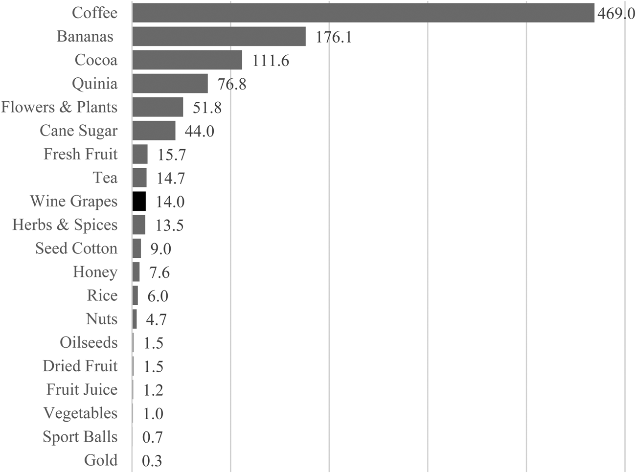
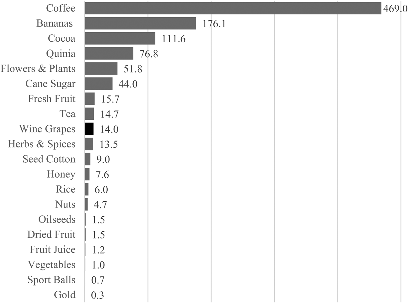
Among FT traded goods, wine grapes and wine play only a minor role. As shown in Figure 1, during the fiscal year 2013–2014, global FT producer wine grape sales accounted for €14 million, significantly behind coffee (€469m) or bananas (€176m).
Global Producer Sale Incomes for Main Fairtrade Goods, 2013–2014 (in million €)
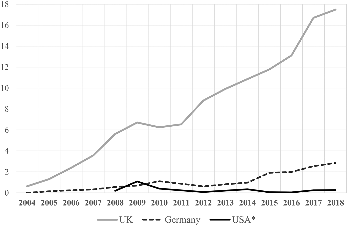
The United Kingdom is the main market for FT wine (Figure 2). Since their UK launch in 2004, the volume of FT wines sold has grown from 620 tons to about 17.5 million liters (2018); in Germany sales rose to almost 2.9 million liters (2018). In contrast, after FT wines were introduced to the United States in 2008, sales quickly rose to 1.1 million liter in 2010, but plummeted thereafter to now 0.25 million liters (2018).. The latest U.S. data report FT sales of 107 tons for 2017, which equals approximately 0.09% of the overall U.S. wine import volume. In 2015, Fair Trade USA suspended its wine portfolio.
Sales of Fairtrade Wines in the United Kingdom, Germany, and the United States (in million liters)

A. The FT Price Floor
In order to achieve their mission and to cover the cost impulse stemming from the certification process and adherence to various social, environmental, and economic standards, FT is financed by two basic components, a minimum price and a fixed price premium allocated by the producers (Linton, Reference Linton2012).
The minimum price has been adjusted only twice in 16 years, in 2004 and in 2014. Since January 2014, the price floor has been set at ZAR 2.19/kg for conventionally grown wine grapes and ZAR 2.57/kg for organic grapes.
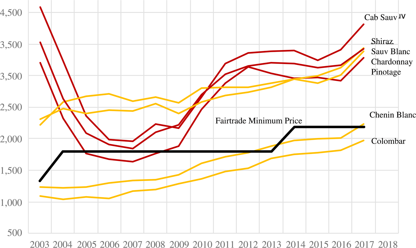
Figure 3 shows average producer cellarFootnote 3 prices for the most popular grape varieties in South Africa. Although producer cellar prices are much lower than trade prices, there are only two grape varieties, Chenin Blanc and Colombar, both white varieties, that are consistently below the current FT price floor. Chenin Blanc is South Africa's most planted wine grape variety and can produce some high quality single-varietal wines. In contrast, Colombar, the second most planted variety, is almost exclusively used in white blends. Among the red wine grape varieties, only Pinotage temporarily broke below the FT price floor. Against this background, we suspect that the predominance of white blends and Chenin Blanc among FT wines (see Section III), and to some minor extent red Pinotage wines, is driven by their low prices. The FT price floor appears to attract the most inexpensive grapes.
Producer Cellar Winegrape Prices and Fairtrade Price Floor in South Africa, 2003–2017 (price in Rand/ton)

B. The FT Premium
The FT premium is paid in addition to the price of a FT product, irrespective of whether the price charged is the Fairtrade minimum price or a higher price. The FT premium is paid directly to farmers to fund projects that address both individual and community needs.Footnote 4 This premium is paid only once, by the first buyer of the product. In the case of unprocessed wine grapes, the Fairtrade premium has been ZAR 0.60/kg since 2014, regardless of whether the grapes were grown organically or not.
In the case of wineries that grow their own grapes, however, the premium becomes payable on the processed product, that is, wine, by the first buyer of the wine, usually an importer, distributor, or retailer. In such cases there is a set conversion rate from unprocessed product to processed product based on average yield. For wine, 1 metric ton of wine grapes is equal to 700 liters of red wine or 630 liters of white wine (Flo-Cert GmbH, Reference GmbH2010). Since January 2014 the premium, based on this conversion, has been set at €0.72/liter for red wine and €0.080/liter for white wine. The reality reported by wineries, however, is that the premium on finished wine is usually incorporated into the price rather than charged to the customer separately. The winery then simply deducts the appropriate amount and transfers it into the communal fund for the workers once the sale has taken place.
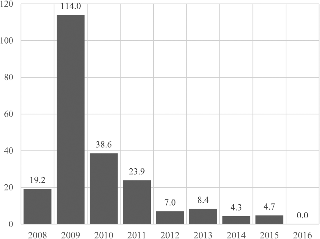
Figure 4 reports the premium payouts resulting from FT wine sales in the United States. The data refer to Fair Trade USA only, and reflect the declining sales pattern after the peak in 2009.
Premium Payments for Wines Sold in the United States
(in $1,000)

The current paper sets out to shed some light on the cost pass-through process along the supply chain. In general, FT-induced cost impulses may be completely passed through, absorbed when the pass-through rate is less than 100%, or amplified when the pass-through rate exceeds 100%. As a result, margins and markups may remain unaffected, negatively affected, or positively affected by the FT treatment. Employing various models, OLS, 2SLS, and propensity score matching (PSM), we find evidence for asymmetric pass-through rates. Our findings suggest that the FT cost effect leaves wholesaler margins unaffected, implying a complete pass-through. In contrast, wine retailers appear to amplify the FT effect resulting in higher margins for FT wines compared to their non-FT counterparts.
The remainder of this paper is organized as follows. Section II discusses the relevant literature and Section III presents the data. In Section IV, we develop a simple theoretical double marginalization model. Sections V to VII report the results of various OLS, 2SLS, and PSM models of prices and margins. Section VIII summarizes and interprets the findings.
II. Literature
There is a large and growing body of literature related to the economics and sociology of Fair Trade in general (see, particularly, Dragusanu, Giovannucci, and Nunn, Reference Dragusanu, Giovannucci and Nunn2014). Naturally, most research focuses on top grossing FT goods, such as coffee, bananas, and cocoa. Here, we will only focus on selection bias issues and possible consumer price effects.
A. Selection
Although, being FT-certified is not a random treatment, it is a priori unclear whether the selection is positive or negative. On the one hand, disadvantaged and less-skilled producers whose products fetch subpar prices may seek certification to benefit from the price floor and improve their position. On the other hand, completing the FT-certification process requires a certain level of organizational skills and consciousness. For coffee growers in Costa Rica, Dragusanu and Nunn (Reference Dragusanu and Nunn2018) find evidence of positive selection. FT-certification is associated with greater environmental and social consciousness and a higher degree of logistical and managerial ability. In contrast, Sáenz-Segura and Zúñiga-Arias (Reference Sáenz-Segura, Zúñiga-Arias and Ruben R2009), Ruben and Fort (Reference Ruben and Fort2012), and Fort and Ruben (Reference Fort, Ruben and Ruben2009) find evidence of negative selection. Examining coffee growers in Costa Rica and Peru, respectively, their results suggest that low levels of education, experience, and income are positively associated with FT-certification.
B. Consumer Prices
In order to be able to pay premiums and above-market prices to growers, it is crucial that the cost impulse is passed on along the supply chain to the end consumer. There is ample evidence that consumers have a favorable view of FT products. For instance, Hainmueller, Hiscox, and Sequeira (Reference Hainmueller, Hiscox and Sequeira2015) ran several in-store experiments and placed FT labels on bulk bins of coffee that were Fair Trade certified. They find that sales grew by 10% if the coffee was labeled as FT. In another experiment examining coffee sold on eBay, Hiscox, Broukhim, and Litwin (Reference Hiscox, Broukhim and Litwin2011) find that consumers are willing to pay an average premium of 23% for FT-labeled coffee.
While there is a substantial body of literature on non-wine FT products (Dragusanu, Giovannucci, and Nunn, Reference Dragusanu, Giovannucci and Nunn2014), the wine-related FT literature on prices is fairly sparse. There is, however, a rich body of price studies on certified sustainable and organic wine. For instance, Corsi and Strøm (Reference Corsi and Strøm2013) find significant (farm gate) price premiums for organic wine in Europe. However, Delmas and Grant (Reference Delmas and Grant2014) find the opposite for the United States. Distinguishing between unpublished eco-certification and published eco-labeling they find that, while eco-certification yields a price premium, the use of the eco-label does not. Drawing on an online survey, Delmas and Lessem (Reference Delmas and Lessem2017) find that eco-certification lowers the probability of choosing the certified wine, particularly in higher price brackets, possibly because the eco-label may be deemed a signal of lower quality.
Similarly, Schäufele and Hamm (Reference Schäufele and Hamm2017, Reference Schäufele and Hamm2018) show an attitude-behavior-gap for German wine consumers. Despite their positive attitude toward sustainable wine, many consumers, especially in lower income brackets, prefer to purchase conventional wine, suggesting the absence of a higher WTP for eco-certified wine.
Niklas, Storchmann, and Vink (Reference Niklas, Storchmann and Vink2017) analyze retail prices of FT wines in the United Kingdom. First, they find a significant price discount for FT wines compared to their non-FT counterfactuals—even after controlling for quality, grape variety, age, and producer fixed-effects. Second, the price dispersion for FT wines appears to be higher than for non-FT wines, suggesting a higher search intensity. These results may indicate that, if the FT cost impulse does not reach the consumer, it must have been absorbed somewhere along the supply chain.
III. Data
Our analysis draws on price data for about 470 South African wines by 11 producers, sold in U.S. wine stores in New Jersey and Connecticut in October and November 2016. The retail data were collected from the website wine-searcher.com (Wine Searcher, 2016), an online site on which more than 10,000 U.S. wine stores post the prices of their wine inventory. All retail prices include the respective state wine taxes but do not include general sales taxes.
Since in both New Jersey and Connecticut the monthly publication of wholesale prices is mandatory, we also have wholesale prices. This allows us to compute wine retail markups for our sample. All wholesale prices are extracted from Beverage Network price books (Beverage Media Group, 2016a; Beverage Media Group, 2016b).
In addition to retail and wholesale prices, we also have import free on board (FOB) prices for most of our sample. These prices, provided by a private shipping company, enable us to compute wholesale margins and markups. However, due to the fact that there is an additional importer-tier before wholesalers, these markups cannot solely be attributed to wholesalers. Instead, it should rather be deemed a combined importer-wholesaler markup.
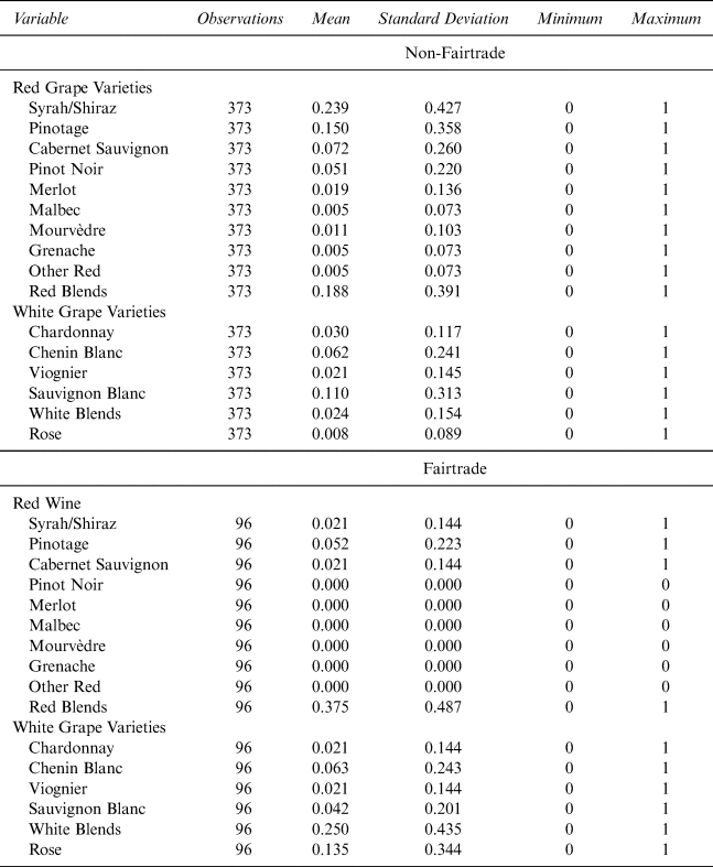
Table 1 provides some descriptive statistics on grape varieties separate for FT and non-FT wine. Since all these variables are 0–1 dummies, the mean value reports the percentage occurrence. For instance, 7.2% of all non-FT wines contain Cabernet Sauvignon, compared to only 2.1% of FT wines. Likewise, 15% of non-Fairtrade wines contain Pinotage, while only 5.2% of Fairtrade wines do. In general, FT wines are predominantly red or white blends. In addition, Fairtrade wines are significantly more likely to be white than are non-FT wines, suggesting that the FT-treatment may be non-random.
Descriptive Statistics: Fairtrade and Non-Fairtrade Wines by Grape Varietal

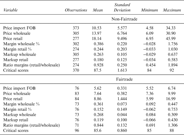
Table 2 reports some descriptive statistics for critical wine scores, which are also from Wine Searcher (2016),Footnote 5 and our dependent variables, that is, prices and margins, also differentiated by FT and non-FT wines. In general, Table 2 exhibits two patterns. First, FT wines cost about half of their non-FT counterparts at all levels (i.e., import, wholesale, and retail). Second, FT wine prices exhibit a substantially lower standard deviation than non-FT wines. This pattern seems to a be a reflection of the respective critical scores. On average, FT wines are rated two critical points lower than their non-FT counterparts and display half their standard deviation.
Descriptive Statistics: Prices, Margins, and Critical Scores

For both FT and non-FT wines, average wholesale margins are significantly higher than retail margins. This appears to be particularly pronounced for FT wines. This is also reflected in the ratio of absolute retail/wholesale margins, which are, on average, smaller than one. While the average ratio equals 0.988 for non-FT wines, it is 0.844 for FT wines.
IV. Three-Tier System, Double Marginalization, and Margins
In 1933, Alcohol Prohibition was repealed by the 21st Amendment, which specifies that the power to regulate alcohol markets resides with the states. As one of the results, all states instated a three-tier system of alcohol distribution.Footnote 6 The three tiers are (1) producers or importers, (2) wholesalers or distributors, and (3) retailers. All alcoholic beverages, that is, wine, beer, and spirits, must successively pass through all three tiers; bypassing any tier is prohibited. That is, importers can only sell to wholesalers who can only sell to retailers. Only retailers are allowed to sell to consumers.
In the three-tier system, with a few exceptions, wholesalers are pure monopolists, that is, in most states, only one wholesaler carries a certain brand. All in-state retailers can purchase only from in-state wholesalers, that is, they must not buy from out-of-state wholesalers. Retailers, however, compete horizontally with other retailers and only enjoy some degree of monopoly power.
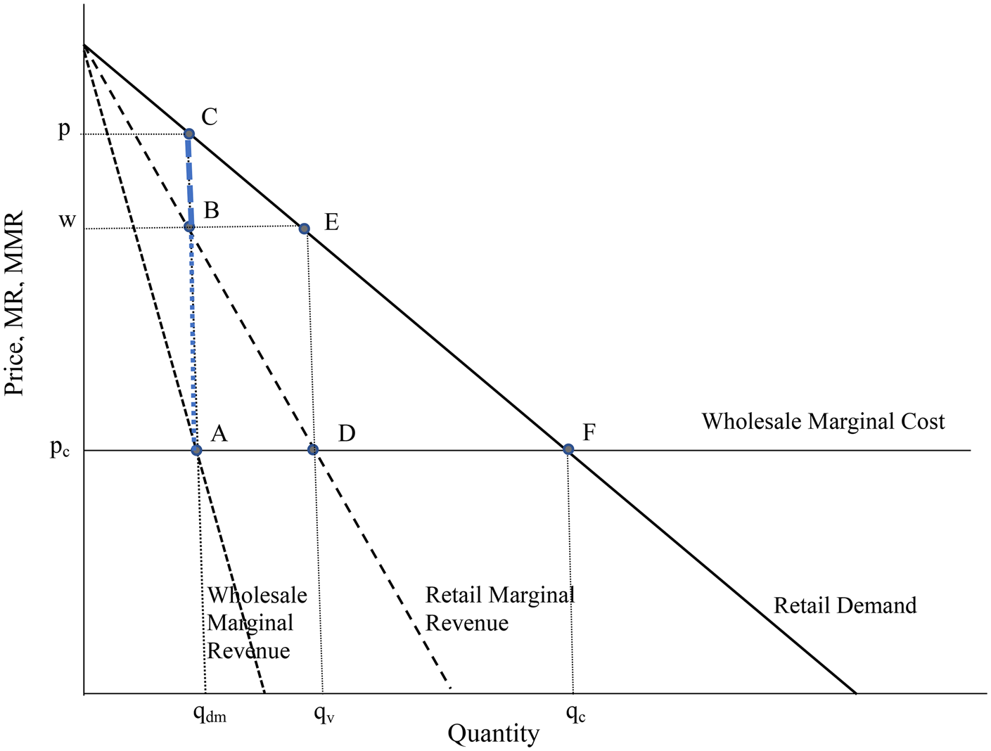
The three-tier structure results in successive monopoly problems that give rise to a double markup on the wholesaler's marginal cost. This phenomenon, first described by Spengler (Reference Spengler1950), is also known as double marginalization. In order to solve the interaction between retailer's and wholesaler's price policies, one solves the retailer's problem first and employs backwards induction to determine the wholesaler's quantity and price. Figure 5 shows the basic idea for the one-product case with a linear demand curve, and assuming that the wholesale price is the only marginal cost to the retailer.
The Double Marginalization Phenomenon
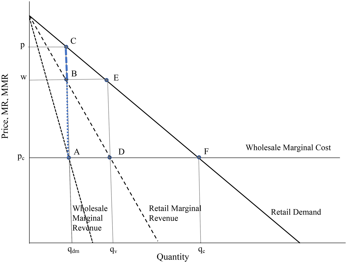
The retailer faces the market demand curve, which is at least twice differentiable, and equates his marginal revenue and marginal cost (here, the wholesale price). The retailer's marginal revenue curve, in turn, becomes the wholesaler's demand curve. He too, equates his marginal revenue and marginal cost, here at point A, which sets the quantity at q dm and the wholesale price at w. The wholesale price becomes the retailer's marginal cost. Following MR = MC, we will get retail price p. The resulting absolute margins, that is, the difference between price and marginal cost, are depicted by the line AB for the wholesaler and BC for the retailer. The deadweight loss is thus given by the triangle ACF.
As can be seen from Figure 5, the double marginalization case if different from vertical integration, when only one monopolist sets quantity and price. The latter case would result in MR = MC at point D with the higher q v and the lower price w. The resulting deadweight loss is smaller than in the unintegrated case and given by the triangle DEF.
For the sake of comparison, point F depicts the competitive solution, with quantity q c and price p c, and no deadweight loss.
There is a large body of literature on the double marginalization problem and its effects on pass throughs and margins (e.g., Bresnahan and Reiss, Reference Bresnahan and Reiss1985; Hong and Li, Reference Hong and Li2017; RBB Economics, 2014, provides a comprehensive survey).
Following Bresnahan and Reiss (Reference Bresnahan and Reiss1985), we decompose our problem into the retailer's selling problem and the wholesaler's pricing problem. The downstream retailer sets his marginal revenue P$\lpar Q \rpar + {\rm Q}\displaystyle{{dP\lpar Q \rpar } \over {dQ}}\;$ equal to his marginal cost, here assumed to consist of the wholesale price (w) and some other idiosyncratic marginal selling cost (s)

The upstream wholesaler's pricing problem is solved by equating marginal revenue and marginal cost:

where MMR(Q) denotes the wholesaler's marginal revenue and c his marginal cost, which comprises the import price, taxes, storage cost, and distribution cost.
The ratio of absolute retailer margins over wholesaler margins can then be expressed as

By dividing by the respective prices, P and MR, we receive the ratio of relative margins as ratio of Lerner indices

where η denotes the respective price elasticities.
Further transforming Equation (3a) yields

where τ denotes the quantity elasticity of the slope of the demand curve. τ summarizes the curvature of the demand curve and determines the distribution of rents between retail and wholesale.
For a linear demand curve, where the second derivative equals zero, τ will always be zero. Therefore, the ratio of margins will always be one-half and the retailer retains only one-third of the entire rent. However, a convex demand curve will yield margin ratios above one-half. Hence an increase in the demand curve's convexity will increase the retailer's rent share.
V. Wine Prices: OLS and 2SLS
We consider prices in two states, Connecticut and New Jersey, that have different alcohol regulations. For instance, while New Jersey's wine tax amounts to $0.88 per gallon, Connecticut's tax is only $0.72 per gallon. In contrast, with $0.24 per gallon, Connecticut's beer taxes are twice as high as New Jersey's.
Similar differences exist for posted wholesale prices. In both Connecticut and New Jersey binding wholesale bottle prices must be posted once a month. Connecticut prohibits wholesalers from granting any further discounts for larger quantities to retail stores (e.g., for the purchase of one or several cases). In contrast, in New Jersey, wholesalers are allowed to grant a price discount for the purchase of one case. Case discounts are posted and binding. Further quantity discounts are prohibited. However, New Jersey's liquor laws include the so-called retail incentive program (RIP). “RIP is a form of rebate in which a wholesaler provides a financial incentive to a retailer to purchase a specific quantity of alcoholic beverages.”Footnote 7 The financial incentive is given upfront and in cash and must not exceed $1,000. For wine, the incentivized quantity must not exceed 50 cases. As a result, RIP is a way to grant discounts for larger quantities and thus circumvent posted wholesale prices. In order to capture these and other state-specific and time-invariant effects we include a dummy variable for New Jersey.
Table 3 reports the results of a few simple OLS price regressions. All equations include a constant term and a full set of producer and varietal dummies (not reported in Table 3). Note, since producers may produce FT wines and non-FT wines at once, the inclusion of producer-fixed effects will not cause any identification problems. The retail equations also contain a set of wine store-fixed effects. All regressions suggest the existence of a significant and substantial FT price premium ranging from approximately 36% to 41%. While import and wholesale price premia are at the lower end of this range, retail premiums appear to be larger than 40%. All prices are also positively associated with critical quality scores. The quality score effect seems to be higher for import and retail prices and somewhat less pronounced for wholesale prices.
OLS Price Equations Dependent Variable ln(Price)

Notes: Robust t-statistics in parentheses. Significance levels 1% (***). All equations include a constant term and a full set of producer and varietal dummies. The retail equations also contain a set of wine store-fixed effects.
Adding a state dummy variable (Table 3, Columns (3) and (5)) yields significant wholesale (approximately 12%) and retail discounts (approximately 5%) for New Jersey—while all other coefficients remain virtually unchanged.
However, as already shown in Section I and Section III, we suspect that the FT treatment is non-random and endogenous. The low price floor and the price premium may attract low price wines made from inexpensive, predominantly white grapes (see Figure 3 and Table 1).
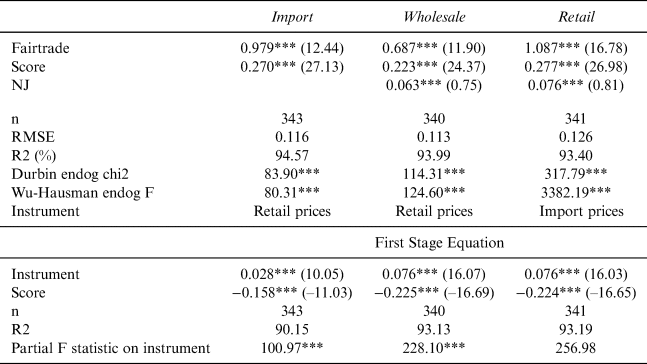
FT wines are of lower quality than their non-FT counterparts, prices are lower too (see Table 1 and 2). We, therefore, assume that our OLS estimates are biased and run a 2SLS model in which upstream prices or downstream prices, respectively, serve as instruments. In particular, we use retail prices as instruments for both import and wholesale prices, and import prices as instruments for retail prices. Table 4 reports the 2SLS as well as the corresponding first-stage results. The Durbin and Wu–Hausman tests for all equations are highly significant, suggesting that we can reject the null of exogeneity of the FT variable. All equations are just-identified and the partial F statistics on the instruments suggest that our instruments are not weak.
2SLS Price Equations Dependent Variable ln(price)

Notes: Robust z-statistics in parentheses. Significance levels 1% (***). All equations include a constant term and a full set of producer and varietal fixed effects. The retail equation also includes retail outlet fixed effects.
As expected, the first stage equations show negative correlations between the FT treatment and quality scores. The positive effect of the price instrument variable on the FT treatment expresses the FT price premium after controlling for all other exogeneous variables, that is, a New Jersey dummy, fixed-effects for producers, varieties, and (in the case of retail prices) also retail outlets.
The 2SLS results indicate that the FT premiums may be significantly higher than suggested by the OLS equations in Table 3; on average, the treatment effects are more than twice as high. However, the fact that retail prices exhibit higher treatment premia than import and wholesale prices remains unchanged. Also, the 2SLS estimates yield marginal quality scores effects that are almost identical with the OLS results.
VI. Margins and Markups: 2SLS
A. Wholesale
Due to the fact that the FT treatment variable appears to be endogenous in the price equations we continue with the instrumental variable 2SLS approach. We estimate various variants with four different dependent variables, that is, margins, markups, and their logarithms. Margins are defined as percentage premium over the purchase prices. For instance, the retail margin is defined as [(retail price/wholesale price) – 1]. The markup is the percentage fractions of the price above marginal cost [(P – MC)/P)]. Accordingly, the retail markup is then [(retail price/wholesale price)/retail price].
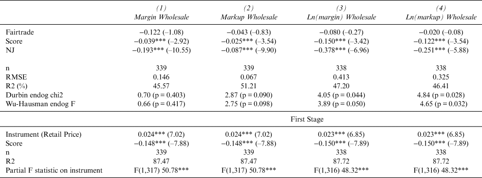
Table 5 reports four 2SLS estimates for the wholesale segment. All equations are just identified, that is, similar to the price equations, we use the retail price as exogenous instrument. The partial F statistics suggest that we have strong instruments. All four variants report insignificant treatment effects on the margins/markup, suggesting that, at the wholesale level, FT wines do not yield profits that are different from their counterparts. In contrast, being located in New Jersey and having high quality scores exert significantly negative effects on margins and markups.
2 SLS Wholesale Margin/Markup Equations

Notes: Robust z-statistics in parentheses. Significance levels 1% (***). All equations include a constant term and a full set of producer, varietal, and retail outlet fixed effects.
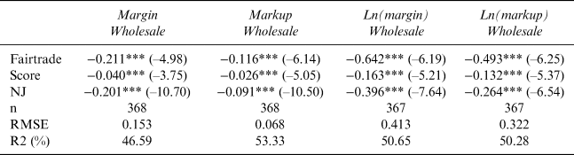
The first-stage results reported in Table 5, however, also show that the treatment may not be endogenous. In particular, the Durbin and Wu–Hausman tests for the margins equation (Column (1)) suggest that we cannot reject the null of exogeneity. We, therefore, also show simple OLS regressions for the four variables in Table 6 and find similar results.
OLS Wholesale Margin/Markup Equations

Notes: Robust t-statistics in parentheses. Significance levels 1% (***). All equations include a constant term and a full set of producer, varietal, and retail outlet fixed effects.
B. Retail
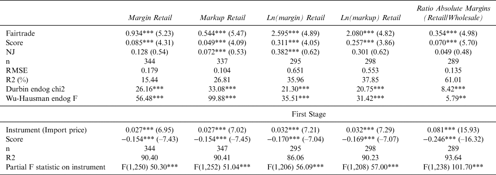
Our retail margin/markup equations, reported in Table 7, follow the same specifications as the wholesale equation, except, instead of retail prices we use import prices as instruments. However, the results are markedly different from those reported in Table 6. In contrast to the wholesale level, we find substantial and statistically significant positive FT treatment effects on retail margins and markups. This applies to both the linear and the logarithmic variants. Accordingly, after controlling for various fixed effects and quality scores, our estimates suggest that FT wines yield margins that are approximately 93% higher than those for non-FT wines. Similarly, markups are about 54% higher. This may appear high, but given the figures provided in Table 2 in Section III, retail margins and markups are in general significantly lower at the retail level than at the wholesale level. This is true for FT and for non-FT wines. For instance, while average wholesale markups lie between 0.263 (non-FT) and 0.268 (FT), average retail markups range from 0.114 to 0.180 (see Table 2). A markup premium of 0.544 for FT wines will, therefore, lift retail markups above wholesale levels.
2 SLS Retail Margin/Markup Equations

Notes: Robust z-statistics in parentheses. All equations include a constant term and a full set of producer, varietal, and retail outlet fixed effects. Significance levels: *** (1%), ** (2%).
In addition to significantly positive FT premiums on retail margins and markups, retail also benefits from higher quality scores. Wine retail markups grow by approximately 4.9% per critical point (note: margins as well as markups are measured in percent). However, given the small range and low level of FT quality scores, the quality effect will mainly be driven by non-FT wines.
In the last column of Table 7, we report the effects of the FT treatment on the ratio of absolute margins (retail/wholesale). As expected, and in accordance with all prior results, being FT exerts a significantly positive effect on the margin ratio.
VII. Wine Margins: PSM
In order to assess the robustness of our findings we also employ a PSM and compare its results with those derived from the 2SLS model reported in Section IV. PSM is aimed at isolating the treatment effect while purging it from other confounding factors (see, also, Rosenbaum and Rubin, Reference Rosenbaum and Rubin1983; Dehejia and Wahba, Reference Dehejia and Wahba1999, Reference Dehejia and Wahba2002; for a wine and restaurant-related example, see Gergaud, Storchmann, and Verardi, Reference Gergaud, Storchmann and Verardi2014).
PSM is designed as a two-step approach. In a first step, we employ a binary probit model to calculate the conditional probability of each observation to be assigned to the treatment group, that is, being FT, given its pretreatment characteristics (propensity score). In step two, we match treated with untreated observations based on their respective propensity scores. This way we create a counterfactual situation which enables us to evaluate the treatment effect for matches with (almost) identical pretreatment characteristics.
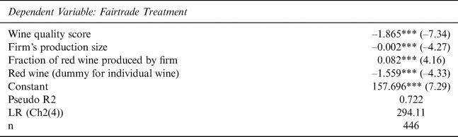
Table 8 reports the results of the probit model for the treatment (i.e., FT) assignment. Accordingly, the probability of being treated grows with decreasing wine quality scores, the smaller the wine-producing firm is, and the higher the firm-specific fraction of red wine production is. In addition, the negative effect of the red wine dummy variable indicates that white wines are more likely to be Fair Trade.
Probit Equation to Generate Propensity Scores

Notes: Robust z-statistics in parentheses. Significance levels 1% (***).
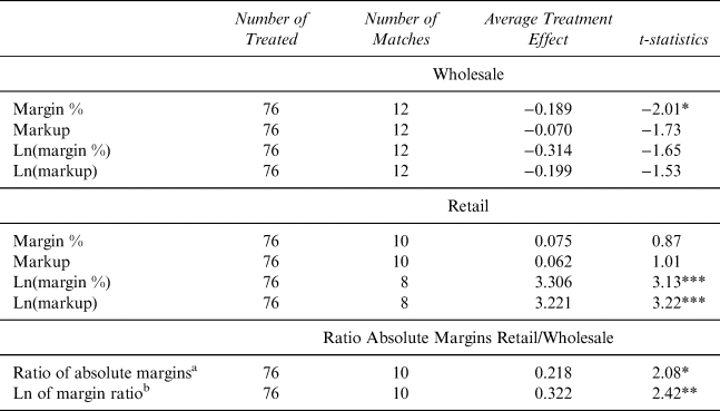
We then selected propensity score matches based on the “nearest neighbor” criterion. Due to the fact that our sample is relatively small, we did not find many matches. For the wholesale model we found matches for 12 of 76 Fair Trade wines. For the retail model we find between 8 and 10 matches, with negative consequences for the respective significance levels.
Nevertheless, the PSM results reported in Table 9, lend further support to our results from Section VI. We find negative average treatment effects for all margin/markup variants at the wholesale level—although the treatment effect attains statistical significance of 5% only for the percentage margin version.
PSM: Wholesale and Retail

Notes: Matches are based on the “nearest neighbor” criterion. Standard errors are based on 100 bootstrap repetitions. Significance levels: * (5%), ** (2%), ***(1%).
a (margin retail/margin wholesale), no bootstrapping.
b ln(margin retail/margin wholesale), no bootstrapping.
In contrast, the average treatment effects for retail margins/markups are all positive and significant at the 1% level for the logarithmic dependent variables. In addition, the retail treatment effects are in magnitude not very different from the 2SLS results. For instance, for the logarithms margin variant, the Fair Trade PSM treatment yields an average effect of 3.22, compared to the corresponding 2SLS effect of 2.6.
Consequently, the ratio of retail over wholesale margin is also positively affected by the FT treatment.
Overall, the PSM model supports our 2SLS findings. While wholesale margins/markups remain largely unaffected by the FT status of a wine, retail margins are a positive function of the FT treatment. In other words, wine stores appear to amplify the FT cost-impulse.
VIII. Conclusion
Our paper sets out to analyze whether and to what extent FT-induced cost impulse can be passed through and whether FT-certified wines affect the margins of wholesalers and retailers differently. Employing various models, that is, OLS, 2SLS, and PSM, we find evidence for asymmetric FT effects. While wholesalers seem to completely pass through the FT effect, leaving their margin unaffected, retailers appear to amplify the FT effect. That is, retailer margins are a positive function of the FT treatment. As a result, the ratio of retailer over wholesaler margin is larger for FT wines than for their non-FT counterparts.
Referring to the theoretical model described in Section IV, our results point to the respective Lerner indices. Given its character as pure monopolist, we assume that the wholesaler's Lerner index is always larger than the retailer's Lerner index. However, our results suggest that this ratio increases for FT wines. Within the context of our theoretical model, this can only be due to a lower elasticity of demand (on the retail market). A possible explanation could be the “warm glow effect” and the resulting higher willingness-to-pay for an ethically superior product. This would contradict Niklas, Storchmann and Vink (Reference Niklas, Storchmann and Vink2017) who found smaller price dispersions for FT wines in the United Kingdom, indicating a higher degree of search and thus higher price elasticities than for non-FT wines. Likewise, Delmas and collaborators (e.g., Delmas and Grant, Reference Delmas and Grant2014; Delmas and Lessem, Reference Delmas and Lessem2017) could not find any “warm glow” price effect for organic wines in the United States.
The fact that our analysis focuses on prices only and disregards quantities sold may obscure the actual market behavior. One may think that a FT wine exhibited in a retail store may only serve as a “warm glow” signal—showing the store's ethical consciousness. It is not meant to be sold but only exerts a positive external effect on the remaining non-FT inventory.
The dramatic decline of the U.S. FT wine market after 2011 may have resulted in fewer stores carrying FT wine, while the number of stores carrying non-FT wines remained constant. This explanation does not assume that it was the amplified pass throughs at the retail level that caused the demise of the FT market but rather vice versa. Fewer FT wine stores with fewer FT wines allow for higher retail prices and margins. Investigating this hypothesis would, however, require a dynamic analysis which is out of the scope of the present cross-sectional snapshot.