

Risk behaviors often occur in escalating sequences. In the case of drug use, this escalation has been conceptualized as a gateway process, wherein marijuana use in particular is thought to pave the way for subsequent use of other, more serious, illegal drugs. According to this gateway hypothesis (Kandel, Reference Kandel1975; Kandel, Yamaguchi, & Chen, Reference Kandel, Yamaguchi and Chen1992), most drug use follows a progressive and structured escalation from tobacco and alcohol to marijuana and then to “hard” drugs such as cocaine and heroin. As it both correlates with and generally precedes hard drug use (Ellickson, Hays, Bell, & Robert, Reference Ellickson, Hays, Bell and Robert1992; for review, see Kandel, Reference Kandel and Kandel2002), marijuana appears to provide a bridge between licit drugs and more severe illicit drugs. By presenting evidence of association and time order, extant research suggests marijuana use may play a causal role in later hard drug use. In this role, marijuana has been framed as a gateway drug.
Despite the reliable association between marijuana and hard drug use, and the fact that marijuana use generally precedes hard drug use, it is difficult to be certain that marijuana use actually causes later hard drug use (Kandel & Jessor, Reference Kandel, Jessor and Kandel2002). Before establishing direct causation, it is necessary to rule out the possibility that other factors, collectively referred to as “third variables,” may influence both behaviors. In the case of the gateway hypotheses, potential third variables include all factors that may contribute to an individual self-selecting into both marijuana and hard drug use (Kandel & Yamaguchi, Reference Kandel, Yamaguchi and Kandel2002). For example, family environmental influences, such as low levels of parental monitoring or exposure to disadvantaged neighborhood contexts, or genetic influences, such as adolescent predispositions toward risk taking, sensation seeking, or depression, may increase adolescents’ likelihood of using both marijuana and hard drugs. To the extent that either family environments or genetics contribute to a behavioral trajectory that includes different types of drug use, the association between earlier marijuana use and later hard drug use could be, at least in part, spurious. Therefore, it is possible that marijuana use both precedes and predicts hard drug use without causing it.
In the present study, we attempt to rule out these two potential sources of spuriousness, family environmental and genetic influences, by applying a genetically informative design to data drawn from the National Longitudinal Study of Adolescent Youth (Add Health). Our design was similar to the discordant-twin control design used by a recent study by Lynskey, Heath, and colleagues (2003) to address the same two sources of spuriousness (see also Lessem et al., Reference Lessem, Hopher, Haberstick, Timberlake, Ehringer and Smolen2006), which used data from both monozygotic (MZ) and dizygotic (DZ) twin pairs to control for household and genetic influences on drug use trajectories. However, Lynskey, Heath, and colleagues (2003) restricted their sample to twin pairs who were discordant for adolescent marijuana use. They found that individual twins who had used marijuana before age 17 were more likely than their nonusing co-twins to use hard drugs thereafter, even after controls.
In our study, we sought to replicate the Lynskey results, but without relying exclusively upon data from discordant twin pairs. Instead, we used data from all same-gender twin pairs available from a nationally representative data set of adolescents. With this expanded sample, we used the magnitude of within-pair differences for adolescent marijuana use, if any, to predict the magnitude of subsequent within-pair hard drug use differences reported during young adulthood.
Prior to summarizing the difference-score approach, data, and measures used by this study, we briefly review the gateway hypothesis, its empirical support, the dual threats of family environmental and genetic spuriousness, and the contributions of Lynskey and colleagues.
The Gateway Hypothesis
The gateway hypothesis was proposed by Kandel (Reference Kandel1975) in the mid 1970s and took on the “gateway” label a decade later. It attempts to account for a consistent pattern: drug use generally begins with either alcohol or tobacco and proceeds, first, to marijuana, and then to other illegal drugs. This pattern is widespread and consistent: evidence suggests 90% of the young adults in the United States who eventually use hard drugs follow this sequence (Kandel, Reference Kandel and Kandel2002). With some exceptions (see Golub & Johnson, Reference Golub and Johnson2002), this pattern has been found among adolescents and young adults of both genderes, irrespective of age of first initiation or ethnic group membership, as well as across different countries and historical periods (for a review, see Kandel & Yamaguchi, Reference Kandel, Yamaguchi, Tarter, Ammerman and Ott1999). Within the category of hard drugs, the order of initiation is less clear, although cocaine more often precedes heroin than the reverse (Newcomb & Bentler, Reference Newcomb and Bentler1986; Sorenson & Brownfield, Reference Sorenson and Brownfield1989). In gateway research, hard drugs are usually aggregated into a single group.
Unlike the older, more deterministic stepping stone theory, which “considered the progression in drug involvement to be inexorable,” the gateway hypothesis is probabilistic: each stage is thought only to increase the risk of entering the next stage of drug use (Kandel, Reference Kandel and Kandel2002, p. 4). Thus, after using marijuana, individuals may or may not progress to harder drugs such as cocaine. Further, it is regular use of marijuana, rather than single or sporadic use, that predicts the progression to hard drugs (Hall & Lynskey, Reference Hall and Lynskey2005).
According to Hall and Lynskey (Reference Hall and Lynskey2005), explanations for the apparent connection between earlier marijuana and later hard drug use generate three broad hypotheses, only one of which would establish a causal connection. The first holds that marijuana users have many more opportunities to try other drugs than nonusers, perhaps because all illicit drugs are “supplied by the same black market” (p. 40), or because a marijuana user's peer group is more likely than a nonuser's to include users of hard drugs. Marijuana users might therefore begin to use hard drugs in response to social norms (Hawkins, Hill, Gui, & Battin-Pearson, Reference Hawkins, Hill, Gui, Battin-Pearson and Kandel2002) or, with increased exposure to drug users, perceive hard drugs as less risky. At least one study has supported this hypothesis: Wagner and Anthony (Reference Wagner and Anthony2002) found that marijuana use increased exposure to, as well as the odds of using, cocaine. However, this hypothesis does not involve a causal connection between marijuana and hard drugs, because the relationship wholly depends upon the context of use and the legal status of each substance. Such contextual third variables could equally affect each member of a household.
The second hypothesis involves intrapersonal third variables, positing that the same individual traits or characteristics that place adolescents at risk for marijuana use also put them at risk for hard drug use. For example, many adolescents may simply enjoy using marijuana, and seek out similar or more intense experiences (Grunberg & Faraday, Reference Grunberg, Faraday and Kandel2002; Lynskey, Heath, et al., Reference Lynskey, Heath, Bucholz, Slutske, Madden and Nelson2003), perhaps after habituating to marijuana use.
The third hypothesis is the only one that is truly causal. It suggests that “the pharmacological effects of cannabis increase an adolescent's propensity to use other drugs” (Hall & Lynskey, Reference Hall and Lynskey2005, p. 40; see Koob, Reference Koob and Kandel2002). For example, marijuana may sensitize the adolescent's brain to the rewards of psychoactive substances, which would make other drugs initially more pleasurable, thereby increasing the risk of continued use (Schenck, 2002). It is of interest that it has also been suggested that other drugs may sensitize the brain as well, making it more amenable to the pleasures of marijuana, in a “reverse gateway” effect (Schenck, 2002, p. 328; see also Patton, Coffey, Carlin, Sawyer, & Lynskey, Reference Patton, Coffey, Carlin, Sawyer and Lynskey2005). All these paths or mechanisms are, of course, probabilistic.
Each of these hypotheses is plausible, and each fits the data. Unfortunately, gateway research has had a difficult time explicitly addressing causality. In the first place, the relevant literature has relied heavily on cross-sectional data, often using Guttman scaling or items that ask about the age of initiation for different drugs to infer order of use (e.g., Kandel & Yamguchi, 2002). In the second place, the studies that have used longitudinal data, although increasing internal validity by demonstrating that marijuana use precedes hard drug use (Ellickson, Hays, & Bell, 1992; Labouvie & White, Reference Labouvie, White and Kandel2002), address only time order but not the potential for spurious causation by third variables.
The Primary Empirical Threat to the Gateway Hypothesis: Third-Variable Spuriousness
Gateway researchers concede that their hypothesis is troubled by third-variable problems. In their recent summary, Kandel and Jessor (Reference Kandel, Jessor and Kandel2002) stated that to interpret the association between the use of one drug and the increased subsequent risk of another as causal, researchers must eliminate alternative influences on the association between these drugs. The most obvious general alternative is that the factors that led to the use of the first drug also influenced the subsequent use of the second drug, in a spurious or third variable model.
Candidates for the role of third variable are numerous. Some operate on the household level. For example, many working or single-parent households may be unable to adequately monitor adolescent children, both in and out of the home, thereby increasing the risk that adolescents reared within them may experiment with drugs. Other parental behaviors, such as modeling illicit and licit substance use or residing in disadvantaged neighborhoods, could also increase adolescents’ exposure to, and risk of using, both marijuana and harder drugs.
Other potential third variables may not be shared by all adolescents in the same household, but may operate at the individual level. For example, an adolescent who is high in sensation seeking, who is open to new experiences, or who desires to self-medicate may be more likely than average to use both marijuana and hard drugs. In addition, many of these characteristics are likely to be genetically influenced. Evidence for genetics as a potential spurious influence on the drugs implicated in the gateway drug sequence comes from twin and adoption studies that suggest that drug using behaviors across substances may have common genetic influences, and further, that these influences appear to manifest, at least to some degree, as increasingly disinhibited behaviors (for review see Hopfer, Crowley, & Hewitt, Reference Hopfer, Crowley and Hewitt2003). Marijuana may be used earlier simply because it is more available and socially acceptable, rendering the gateway sequence “a progression of convenience” (Schenck, 2002, p. 330; see also Clayton, Voss, & LoScuito, 1988; Golub & Johnson, Reference Golub and Johnson2002; Hawkins et al., Reference Hawkins, Hill, Gui, Battin-Pearson and Kandel2002).
It is important to emphasize that being able to list possible third variables is different from being able to effectively control for them. According to Kandel and Jessor (Reference Kandel, Jessor and Kandel2002), the standard approach of statistically controlling for processes that may influence the association between the use of both drugs does not solve the problem, for at least two reasons. First, it is unlikely that all relevant variables that influence adolescent and young adult drug use can be statistically controlled for in a single study. A study demonstrating that the prediction of later hard drug use from earlier marijuana use withstood statistical controls for household supervision or sensation seeking, for example, could be said to rule out potential spurious influences only if these variables, as measured, represented all plausible third-variable threats. Second, gateway researchers who have pursued statistical control have focused on individual adolescents at the expense of the ecological experiences and contexts that surround drug use, usually entering only a handful of sociodemographic variables to control for these processes, despite the profound effect that context may have on the gateway sequence. In inner-city New York, for example, marijuana use often precedes the use of alcohol and tobacco, as well as hard drugs, and many adolescents skip gateway drugs altogether and begin their substance use with hard drugs (Golub & Johnson, Reference Golub and Johnson2002).
To address these concerns, Kandel and Jessor (Reference Kandel, Jessor and Kandel2002) suggested that gateway research would benefit greatly from the application of genetically informative designs, such as twin and adoption studies. In general, design-based controls are superior to statistical controls in establishing internal validity (Shadish, Cook, & Campbell, 2002). In this vein, our design, as well as the discordant twin-control design used by Lynskey, Heath, and colleagues (2003), can be viewed a genetically informative version of the quasiexperimental sibling cohort design.
The Contribution of Lynskey and Colleagues
Following Kandel and Jessor's call for genetically informative research, Lynskey, Heath, and colleagues (2003) used a discordant twin control design to address the family environmental and genetic third-variable threats to gateway drug theory. The Lynskey sample contained 311 twin pairs, both MZ and DZ, reared within the same households. Within each pair, twins were discordant for marijuana use before their 17th birthdays.
To examine the possible effect of shared household membership on the association between early marijuana and later hard drug use, Lynskey, Heath, and colleagues provided the following hypothesis: if the gateway sequence was actually a product of the shared household environment, then the later hard drug use of twins raised within the same household should have been similar despite their earlier discordance for marijuana use, because both twins would have been subjected to nearly identical household-associated environmental risk factors for using hard drugs. Both twins in each pair, the early marijuana user and the nonuser alike, would have been exposed to similar levels of parental supervision, parent behaviors, neighborhood disadvantage, and other potential environmental third variable influences. If these shared household influences contribute to a trajectory that begins with marijuana and continues on to hard drugs, the initial use of marijuana by one twin, an unshared environmental influence, would not predict higher levels of subsequent hard drug use for that twin.
The other third-variable hypothesis Lynskey, Heath, and colleagues examined was that genetic influences were responsible for the progression from marijuana to hard drug use. To test this hypothesis, they compared the results across different zygosity levels of twin pairs. Among DZ twins, who on average share only half of their genetically based risk and protective factors for hard drug use, the differences in genes could explain both initial discordance in marijuana use and subsequent differences in hard drug use (Lynskey, Heath, et al., Reference Lynskey, Heath, Bucholz, Slutske, Madden and Nelson2003, p. 428). Among MZ pairs, however, who share all of their genetically based risk and protective factors for hard drug use, the genetic hypothesis predicted that genetic influences would produce “equal risks” for later hard drug use for each twin within a pair, regardless of twins’ earlier marijuana use discordance. Accordingly, finding that initial marijuana use predicted higher later hard drug use only among DZ, but not MZ, twin pairs would indicate that genetics influence the marijuana to hard drug use trajectory.
In the Lynskey study, the gateway hypothesis survived the challenges presented by both the shared environment and genetic third-variable hypotheses. Its overall finding was that twins who had used marijuana before age 17 displayed greater lifetime hard drug use than their nonusing co-twins, with increased odds ranging from 2.2 for any illicit drugs to 5.2 for hallucinogens. In other words, differences between twins in their initial marijuana use predicted subsequent differences in their hard drug use. Thus, the shared environmental hypothesis was rejected because twins who differed in earlier marijuana use also differed in later hard drug use, despite exposure to shared household environments, whereas the genetic hypothesis was rejected because earlier marijuana differences predicted later hard drug use differences similarly across zygosities, as both DZ and MZ twin pairs demonstrated the gateway effect. Together, these results suggested that the association between earlier marijuana use and later hard drug use was because of the former triggering an increased likelihood of the latter.
Limitations of the Lynskey Study
Although the Lynskey study provided considerable support for the gateway hypothesis, it contained at least three important shortcomings. First, by using only discordant twins, one twin within each pair was required to have reported marijuana use. Second, the study was not longitudinal, as measures of the twins’ earlier marijuana use were based on retrospective data collected up to 15 years after adolescence (McLeod, Hickman, & Smith, Reference McLeod, Hickman and Smith2003). Third, data were derived from uncorroborated self-reports collected via phone interviews (McLeod, Hickman, & Smith, Reference McLeod, Hickman and Smith2003).
The first shortcoming, sampling only discordant pairs, creates two potential problems. By excluding twin pairs concordant for nonuse, the design ensured that the level of substance use among the sample was very high, thereby creating challenges for generalizing results to the population at large (Schier, Nelson, & Hoffman, Reference Schier, Nelson and Hoffman2003). However, considering this shortcoming in the context of the study's design may work to neutralize this objection. By requiring that one member of each twin pair report marijuana use, Lynskey, Heath, and colleagues (2003) selected a high-risk sample (see Lynskey, Statham, et al., Reference Lynskey, Statham, Martin, Heath, Bucholz and Madden2003), a purposive sample strategy that directly led to the study's strength: its ability to reduce the spurious threats of shared family and genetic influences.
Perhaps of greater concern than the design's effect on generalizability, it may be that discordant twin pairs differ in relevant ways from concordant pairs. If so, including only discordant twin pairs seems especially problematic for MZ twins, who are presumptively more similar, and among whom discordance may be the exception, not the rule. Thus, Lynskey, Heath, and colleagues (2003) this may have created a sample of twin pairs unrepresentative not just for level of substance use, but for pair-level patterns of behavior, possibly introducing unmeasured sampling biases that may have influenced their results.
Taken together, the second and third shortcomings, relying on retrospective uncorroborated self-reports of behaviors that occurred up to 15 years prior, threaten the measurement validity of the Lynskey study. Respondents who used marijuana as adolescents but did not use hard drugs as adults may have chosen to dismiss their adolescent marijuana use as experimental or otherwise not important, salient, or even memorable. This could have led to considerable retrospective underreporting of adolescent marijuana use. In contrast, respondents who used hard drugs as adults may be more likely to admit adolescent marijuana use, perhaps because their earlier marijuana use appears to them to be part of a larger pattern of behavior, whether “experimental” or habitual. Although it cannot be determined if or to what extent these possible confounds influenced their results, the potential of retrospective bias suggests some caution should be used when considering the Lynskey results.
Applying a difference score approach
In the present study, we attempted to address each of these shortcomings while retaining the methodological logic of the Lynskey study. Like Lynskey and colleagues, we used between-twin differences in adolescent marijuana use to predict later hard drug use within twin pairs, interpreting the gateway hypothesis to imply that pairs with different levels of earlier marijuana use would report different levels of later hard drug use, regardless of shared genetic or environmental influences.
To address the first shortcoming, the use of only discordant pairs, we decided to use data from all available same-gender twin pairs with valid adolescent marijuana use and later hard drug use scores. Instead of dichotomous measures, we employed continuous measures of substance use, which allowed us to apply a difference score, rather than a discordant pair, approach. Because there is some controversy about difference scores, a brief discussion is warranted. Concerns about these scores center on their reliability. Specifically, these scores can have reliability problems when two conditions co-occur. These two conditions are when (a) component scores themselves have high measurement error and (b) the differences between the two component scores are small (Rogosa, Brandt, & Zimowski, Reference Rogosa, Brandt and Zimowski1982). Although the co-occurrence of these conditions would seem rare, both are possible when difference scores are used to assess within-person change. Unfortunately, they are often used for this purpose, and as a result of being commonly exposed to these statistical conditions have an exaggerated reputation for poor reliability. Outside of this application, however, this reputation is largely undeserved. As shown by Rogosa and Willet (Reference Rogosa and Willett1983), these scores, even when used for the relatively vulnerable within-person change application, can have respectable reliability. The current study does not use difference scores to assess within-person change. Here they are used to capture within-twin pair (i.e., across twin) differences. Unlike within-person change, which can be both systematically small and similar across analysis units (i.e., participants), across-twin differences are often both substantial and different across analysis units (i.e., twin pairs).
Applying a difference score approach allowed this study to use all Add Health same-gender twin pairs with valid marijuana and hard drug data. Doing so maximizes the advantages of the Add Health in a way that addresses the sampling shortcomings inherent in the Lynskey design. The levels of substance use reported by the twin pairs used in the analyses could be compared to the overall substance use rates of the full Add Health sample, which is demographically similar to the American adolescent high school population (Bearman, Jones, & Udry, Reference Bearman, Jones and Udry1998). Thus, the characteristics of the individual twins used in the analysis provided greater potential for generalizability than the highly selected sample used by Lynskey and colleagues. In addition, by not restricting our sample to discordant pairs, we avoided selecting out those (likely more representative) MZ twin pairs with concordant patterns of earlier marijuana use.
The advantages of the Add Health
To address the second and third shortcomings, the use of uncorroborated cross-sectional data with retrospective reports of earlier marijuana use, we used longitudinal data: three waves from the nationally representative Add Health (Bearman et al., Reference Bearman, Jones and Udry1998). By taking advantage of the longitudinal design of the Add Health, we were able to avoid the measurement error specifically associated with retrospective reports of long-past drug use. Although our study, like Lynskey, did use uncorroborated self-report data, most of these data were collected from adolescents about adolescent behavior within the year immediately preceding the data collection, rather than from adults about adolescent behavior. Thus, these data were not as susceptible to the systematic bias caused by viewing earlier marijuana use through the lens of subsequent hard drug use behaviors. In addition, although uncorroborated self-report was used, the data were collected using the Add Health's Audio-Computer Assisted Self-Administered Interview (CASI) procedure, whereby respondents listened to questions about drug use through headphones and entered responses into a laptop computer, instead of responding directly to an interviewer.
We were also able to use the Add Health to go beyond the design-based controls for family environment and genetics that are at the core of our analyses, as well as those of the Lynskey study, by using measures of friends’ marijuana use and respondents’ own hard drug use. These statistical controls for potential third variables supplement the design-based strengths of the twin pair difference score model and further increase the internal validity of our study.
Study Hypotheses
The Lynskey study set out to test alternatives to the gateway hypothesis, but found support for the existence of a gateway effect. Accordingly, we proposed four hypotheses that would imply, if supported, the causal validity of that effect.
Hypothesis 1
Earlier marijuana use differences will predict later hard drug use differences within twin pairs from the same households. If individual twins’ earlier marijuana use, rather than environmental influences associated with the household shared with their co-twins, leads to their later hard drug use, twins with greater earlier marijuana use than their co-twins will go on to greater hard drug use. Thus, the direction and degree of earlier within-pair marijuana use differences will predict the direction and degree of later hard drug use differences among twin pairs. Alternately, if influences associated with household membership, such as similar levels of parental supervision, parent behaviors, and neighborhood disadvantage, are responsible for the marijuana to hard drug trajectory, initial within-pair marijuana use differences will not predict within-pair hard drug use differences.
Hypothesis 2
The association between earlier marijuana and later hard drug use will persist after controlling for differences in earlier hard drug use that was reported concurrently with the earlier marijuana use. This control reduces the chance that later variation in hard drug use results from earlier hard drug use, rather than the marijuana use that began their hypothetical gateway experience.
Hypothesis 3
The association between earlier marijuana and later hard drug use will persist after controlling for differences in exposure to friends’ marijuana use. Such exposure could constitute an alternative third variable, not necessarily shared among household members, affecting the initiation of both marijuana and hard drug use.
Hypothesis 4
Earlier marijuana use differences will predict later hard drug use differences similarly across twin pair zygosity levels. If earlier marijuana use triggers later hard drug use, twins with greater earlier marijuana use than their co-twins should go on to greater hard drug use regardless of their degree of relatedness. However, if genetic influences account for the association between earlier marijuana use and later hard drug use, initial within-pair marijuana use differences would not predict subsequent within-twin pair hard drug use differences for MZ twin pairs, because each twin would be subject to identical genetic influences (Lynskey, Heath, et al., Reference Lynskey, Heath, Bucholz, Slutske, Madden and Nelson2003). Among DZ pairs, however, genetic differences could explain both initial differences in marijuana use and subsequent differences in hard drug use between twins.
Method
Participants and data collection procedure
The current study used twin data available within the Add Health, a national sample of adolescents enrolled in US secondary schools. The Add Health is representative of American high school students in 1995 with respect to region, school type, school size, urbanicity, and ethnicity (Bearman et al., Reference Bearman, Jones and Udry1998). In addition to an in-school data set (N = 90,000), collected during 1995, the Add Health also includes three waves of in-home data: Wave 1 (1995; N = 20,000), Wave 2 (1996; N = 14,500), and Wave 3 (2001; N = 15,500). Data from each of the three waves of in-home data collections were used for this study. Analyses in this study used same-gender MZ and DZ twin pairs drawn from the Add Health's sibling data set, which provides links that allow the construction of twin, full-sibling, half-sibling, cousin, and unrelated pairs living within the same households.
The in-home collections contain data from 760 pairs of twins. After removing the 205 opposite gender twin pairs, 555 pairs were eligible for analyses. Of these, we eliminated 45 pairs: 5 for missing later hard drug use data and 40 for missing earlier marijuana use data. This left a final sample for analysis of 510 twin pairs, 285 MZ and 225 same-gender DZ, who had complete earlier marijuana use and later hard drug use data for each twin. We compared the 40 pairs who were dropped for missing earlier marijuana use data to the final sample, and found that the dropped pairs had significantly (p ≤ .05) higher levels of later hard drug use, .525 (SD = .933) and .625 (SD = .999) for twins 1 and 2, compared to .218 (SD = .589) and .261 (SD = .648) for the 510 retained. Despite these differences, their exclusion had little impact on the analyses. Adding their data back in (N = 550) increased levels of later hard drug use to .240 (SD = .625) and .287 (SD = .686), values that are only .04 and .03 SD, respectively, greater than those of the analysis sample.
The analysis sample was ethnically diverse: 54% White, 23% African American, 15% Hispanic, 5% Asian, and 3% American Indian or other (the Add Health contains an oversample of African Americans). Most in-home interviews took place during the summers of 1995 (Wave 1), 1996 (Wave 2), and 2001 (Wave 3). However, Wave 3 data collections tended to take place later in the summer and in the following months (July was the modal month, compared to June and May for Waves 1 and 2). At the time of different in-home data collections, the average ages of the analysis sample were 16.09, 17.00, and 22.43 (SD = 1.59). The ranges for ages for each wave were fairly substantial, 12.64–19.64, 13.55–20.55, and 18.98–25.98, across waves, respectively. However, as shown by the substantially closer values defining the corresponding interquartile ranges (14.89 and 17.31, 15.80 and 18.22, and 21.23 and 23.65), age of participants tended to cluster around the sample's means at the different waves.
In-home data were collected during 2-hr home interviews using an audio-CASI, during which respondents listened over headphones to tape recorded items and entered responses directly into a laptop computer. Add Health data collectors used this procedure for items that addressed sensitive topics, such as delinquent, sexual, and health behaviors, to which respondents might have responded less honestly were they communicating directly with data collectors.
Measures
Earlier marijuana use differences
We constructed a variable called earlier marijuana differences by subtracting the score of Twin 2 from Twin 1 on each twin's responses to the Wave 1 item, “During your life, how many times have you used marijuana?” The frequency of lifetime marijuana use ranged from 0 to 500 times for Twin 1 and 0 to 900 times for Twin 2. Both twins’ distributions were highly skewed, with only 8 and 7, respectively, reporting using marijuana over 100 times at Wave 1. To reduce skew, both twins’ individual scores were square root corrected. The resulting range was 0 to 22 for Twin 1 and 0 to 30 for Twin 2. The corrected score of Twin 2 was then subtracted from that of Twin 1 to create a difference score for earlier marijuana use, with a range from −30 to 20. The distribution of the resultant variable, earlier marijuana differences, was symmetrical. Among the 510 pairs with complete data for marijuana use frequency, 67.3% (343) pairs had a score of 0, indicating no difference in earlier marijuana use for these pairs. Sixteen percent (16.1%) of pairs had negative difference scores, indicating greater Twin 2 use, and 16.5% had positive scores, indicating greater Twin 1 use.
Later hard drug differences
Twin pairs’ later (post-Wave 1) hard drug use difference score was constructed from each twins’ responses to both Wave 2 and Wave 3 items assessing hard drug use. The specific items were similar, but not identical, across data collections. In Wave 2, respondents were asked to respond to items asking whether, since the date of the last interview, they had (a) used cocaine; (b) used inhalants, such as glue or solvents; (c) used any other type of illegal drug, such as LSD, PCP, ecstasy, mushrooms, speed, ice, heroin, or pills, without a doctor's prescription; and/or (d) injected an illegal drug, such as heroin or cocaine. In Wave 3, respondents were asked similar questions: whether since June 1995, the average date of the Wave 1 interview, they had (a) used cocaine, including crack, freebase, or powder; (b) used crystal meth; (c) used other types of illegal drugs, such as LSD, PCP, ecstasy, mushrooms, inhalants, ice, heroin, or prescription medicines not prescribed to you; or (d) injected (shot up with a needle) any illegal drugs. Responses to these eight Wave 2 and Wave 3 items were used to assign each twin a score for hard drug use since 1995. Because respondents were reporting twice on the same drug (except for inhalant use at Wave 2 and crystal meth at Wave 3, we first created four separate hard drug use indicators: (a) cocaine, (b) inhalant/meth, (c) other illegal drugs, and (d) injected drugs. Summing across Waves 2 and 3, the most commonly used category of hard drug was “other illegal drugs” with 140 (14%) of the 1,020 twins reporting some use since Wave 1, followed by 50 (5%) reporting cocaine use, 49 (5%) reporting inhalant/meth use, and 6 (1%) reporting injected drugs. For each twin, individual usage scores ranged from 0 to 4 (0 = no use, 4 = use of each of the four hard drug types since 1995). We used these individual scores to create a variable representing later hard drug differences, subtracting Twin 2’s total substance use reported since 1995 from the corresponding Twin 1 substance use score. Values ranged between −3 and 4. The distribution was symmetrical, with 10% of twin pair scores indicating greater use by Twin 2 and 9% indicating greater use by Twin 1.
Control variables
We also created two primary control variables, measuring differences within twin pairs for earlier hard drug use and earlier peer marijuana use. Affirmative responses to Wave 1 items asking respondents about their hard drug use, using cocaine, inhalants, or other types of illegal drugs, and injecting any drugs, were summed to create an earlier hard drug use score for each twin. As with later hard drug use, an earlier hard drug differences variable was constructed by subtracting Twin 2’s score from Twin 1’s score. The distribution of the resulting variable was symmetrical and ranged between −3 and 3. As expected for a relatively rare behavior, 87% (441) twin pairs scored 0, indicating no difference between each twin's earlier hard drug use, with only 6 and 7%, respectively, taking on negative and positive values.
The second control variable, earlier peer marijuana differences, was similarly constructed. It was based on responses to a single Wave 1 item, “Of your three best friends, how many use marijuana at least once a month?” The distribution of this variable was symmetrical and ranged between −3 and 3. Among the 510 pairs used in the analyses, 65% (331) scored zero, with 16 and 19%, respectively, taking on negative and positive values.
A third set of variables was constructed to control for age of first marijuana use. Constructing these variables was problematic. Obviously, not all members of the sample had used marijuana, either at Wave 1 or eventually. For example, at Wave 1, 387 of 510 Twin 1’s (75.9%) had not used marijuana and had a value of 0 for the item assessing age of first use. In contrast, of those who had used marijuana, age of use ranged from five respondents reporting use at age 18 (perhaps less risky use) to seven respondents who indicated use beginning before age 10 (presumptively more risky use). Obviously, if those who had not used marijuana at Wave 1 were assigned missing values the resulting variable could not be used in this study's regression models.
To take this missing value problem into account, two approaches were used. The first, creating raw age of use scores, was to assign a value of 20, the age 1 year older than all respondents at Wave 1, to all who reported no use at Wave 1. This assignment, and then setting to 11 of all values ≤11, created a distribution from 11 to 20, with the value of 20 indicating no use reported at Wave 1. In the second approach, we created probability of use scores by assigning values to each respondent based on the sample's probability of use at the age the individual respondent reported first use. For example, only 3% of the sample reported marijuana by age 11. Those who reported use at that age were assigned a value of .97, based on the likelihood of that use subtracted from 1 (1 − .03 = .97). By subtracting from 1, we allowed the variable to correlate with later hard drug use in the expected (positive) direction. The value assigned to those who reported no use at Wave 1 was the overall probability of use in the sample as reported at Wave 3, which was .49, subtracted from 1.0. The resulting probability of use scores scale ranged from .97 (very early use) to .51 (no use at Wave 1). As with other scales, Twin 2s score was subtracted from Twin 1’s score to construct a marijuana onset differences variable. Both versions of this scale were used in a supplemental analyses to control for age of onset on primary analyses.
Results
Preliminary analyses: Levels of substance use
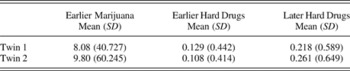
Table 1 provides means and standard deviations for the individual substance use scores for each twin. Unlike the difference score variables, which were symmetrically distributed, these scores exhibited substantial positive skew. This skew was expected, given the nature of substance use behaviors and its continuous measurement (i.e., “During your lifetime, how many times have you used marijuana?”). As noted in Table 1, square-root adjustment reduced this skew substantially. Table 1 also illustrates that the twins’ means for later hard drug use were approximately double the levels of earlier hard drug use.
Reports of adolescent marijuana use and later hard drug use

Note: After square-root adjustment, early marijuana use means were 0.985 (SD = 2.669) and 1.03 (SD = 2.962).
We compared our sample means with means for the full Add Health In-Home sample, and found them to be similar. For example, although the 8.94 average of the twins’ individual marijuana use means was 1.45 lower than the full sample mean (N = 19,994, M = 10.39, SD = 54.34), this difference (10.39–8.94) was only 2.6% of the full sample standard deviation.
Primary analyses: Difference score models
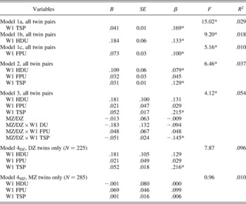
Primary analyses used regression models to examine associations between the difference scores for earlier marijuana and later hard drug use. Table 2 provides the results for the seven models used for the primary analyses. The first, Model 1a, regressed later hard drug differences on earlier marijuana differences, revealing that within-pair differences in Wave 1 marijuana use predicted Wave 3 differences in hard drug use, F (1, 508) = 15.02, p < .05; β = .17. Variance accounted for by Model 1a was .029. This result supported Hypothesis 1, that earlier marijuana use differences would predict later hard drug use differences. This finding refutes the idea that environmental influences associated with household membership were responsible for the association between earlier marijuana use and later hard drug use.Footnote 1
Models 1b and 1c examined the independent association between the control variables and later hard drug differences. Within-pair differences in both their earlier hard drug use, F (1, 508) = 9.20, p < .05; β = .13, and the marijuana use of their closest friends, F (1, 508) = 5.16, p < .05; β = .10, predicted differences in their own later hard drug use.
The prediction of twin pair differences in later hard drug use (N = 510) by Wave 1 marijuana use differences

Note: W1, Wave 1; TSP, times smoked pot; DU, drug used; FPU, friends' pot use; MZ, monozygotic; DZ, dizygotic.*p < .05.
Model 2 examined the association between earlier marijuana differences and later hard drug differences, while controlling for both earlier hard drug differences and earlier peer marijuana differences, F (3, 506) = 6.46, p < .05. The coefficient for earlier hard drug differences was significant (β = .08, p < .05). More importantly, even in the presence of these control variables, earlier marijuana differences still significantly predicted later hard drug differences (β = .13, p < .05). This result supported Hypotheses 2 and 3 that earlier marijuana use differences would predict later hard drug use differences controlling for both differences in concurrent hard drug use and exposure to friends’ marijuana use. However, although earlier hard drug differences was significant, earlier peer marijuana use differences was not. In fact, compared to Model 1a (R 2 change = .008, .037–.029) the increase in variance was not significant, F (2, 506) = 2.10, p > .05, indicating that “as a pair” the addition of these two controls did not significantly increase explained variance.
To examine Hypothesis 4, that earlier marijuana differences would predict later hard drug differences similarly across twin pair zygosity levels, Model 3 added interaction terms examining the similarity of Model 2 parameters across levels of twin zygosity, as well as a dummy-coded main effect for zygosity. The resulting model was significant, F (7, 502) = 4.12, p < .05. The two interactions involving earlier hard drug differences and earlier peer marijuana use differences were not significant. However, the term testing the interaction between level of twin zygosity (MZ = 1, DZ = 0) and earlier marijuana use difference was significant (β = −.15, p < .05), indicating that the association between earlier marijuana differences on later hard drug differences differed according to the degree of genetic relatedness. Perhaps because two of the three added interactions terms were nonsignificant, the increase in variance explained compared to Model 2, although improving nearly 50% from .037 to .054, was not significant, F (4, 505) = 2.27, p = .06. To confirm that the lack of significant increase in R 2 was because of the inclusion of the interactions associated with the control variables, we ran a paired down version of Model 3. This simplified model, which included only the main effects for earlier marijuana difference and twin zygosity and the interaction between them, was significant, F (3, 506) = 7.63, p < .05. Moreover, the R 2 for this model (.043), was significantly greater, F (2, 507) = 3.70, p < .05, than the R 2 of Model 1a (.029). The significant interaction term between zygosity and earlier marijuana difference in Model 3, together with the significant increase in explained variance because of this interaction in the simplified Model 3, led us to reject Hypothesis 4.
To explicate the meaning of the significant interaction between level of twin zygosity and earlier marijuana difference, Model 2 was run separately on DZ and MZ pairs. The results for these models, Models 4DZ and 4MZ, appear at the bottom of Table 2. Results for Model 4DZ, F (3, 221) = 7.87, p < .05, run on DZ twins only, appear similar to those for all twin pairs (Model 2): earlier marijuana differences predicted later hard drug differences (β = .22, p < .05), but other independent variables were not significant. Results differed markedly for MZ twins (Model 4MZ). Neither the full model, F (3, 281) = 0.96, p > .05, nor earlier marijuana differences (β = .01, p > .05) was significant. The differences in results between the DZ and MZ twin types is underscored by the variance accounted by the model for each twin type: .096 among DZ twins but only .010 among MZ twins. In sum, twin pair differences in earlier marijuana use predicted later hard drug use differences only among twins with genetic differences. In contrast, among the genetically identical MZ twins, earlier marijuana use differences did not predict later hard drug use differences. Thus, findings supporting the gateway role of marijuana appear to depend upon genetic influences that are not part of the gateway hypothesis.
Supplemental analyses: Gender, age of onset, and discordant pairs analyses
To address concerns about gender, age of onset, and differences between our results and prior studies, we undertook several additional examinations. First, we considered whether Wave 1 difference scores predicted differently for male–male and female–female pair type. Although significant overall, F (7, 502) = 3.48, p < .05, this analysis did not reveal any significant interactions by gender.Footnote 2
Second, we tested whether our results were affected by our use of participants 17 and older. Ages in Add Health Wave 1 ranged from 12.64 to 19.64, whereas the Lynskey study measured adolescent marijuana use only before age 17. We reran all models after first dropping all twins who were older than 18.0 at Wave 1 (reducing the sample size to 443) and then dropping all twins who were older than 17.0 at Wave 1 (reducing the sample to 350). Even in the face of these age restrictions and smaller sample sizes, our results were unchanged.
Third, as previous research has emphasized the importance of age of onset (Labouvie & White, Reference Labouvie, White and Kandel2002), we reran Models 1a and 3 with the addition of marijuana onset differences, constructed from the probability of use version of our age of first marijuana use variable. Before doing so, we ran a model using marijuana onset differences to predict later hard drug differences. This model, identical in structure to Model 1a (see Table 2), regressed later hard drug differences on age of onset differences, revealing that within-pair differences in Wave 1 reports of age at first marijuana use predicted Wave 3 differences in hard drug use, F (1, 508) = 7.98, p < .05; β = .12. Variance accounted for by this model was .017, which is less than the variance accounted for by the primary independent variable alone (earlier marijuana use). The results from rerunning Model 1a with the marijuana onset differences score covariate revealed that earlier marijuana use difference retained its significant association with Wave 3 differences in hard drug use, F (2, 507) = 7.87, p < .05; β = .15. Similarly, the parameter for the interaction term between level of twin zygosity and earlier marijuana use difference retained its significance when marijuana onset differences and the corresponding age of use by zygosity interaction variable were added to Model 3. Models repeated using raw age of first use difference score provided similar results.
Two shortcomings of the age of onset variable should be noted. First, as it was constructed from items available in the Wave 1 questionnaire, it only assessed the age of first use, but not the intensity of initial use (Labouvie & White, Reference Labouvie, White and Kandel2002). Second, as not all participants who would, or will, go on to use marijuana had done so by Wave 1, both versions of the age of onset control variable were imperfect. For these reasons, although these post hoc analyses strengthen our confidence in the findings, we excluded the age of onset marijuana use variable from our primary analyses.
As an additional check, models were rerun using a version of the outcome that used Wave 3 meth use alone, rather than the combination of Wave 2 inhalant and Wave 3 meth use. Using this outcome did not change the results. In particular, consistent with our other results, the interaction term in Model 3 for zygosity by earlier marijuana use was significant at the .05 level.
Finally, to increase our confidence that the different results are because of our different approach, rather than different samples (the Add Health vs. the Australian Twin Panel Study used by Lynskey) or different measures, we replicated the approach of the Lynskey study using Add Health data. To do so, we identified 41 MZ and 64 DZ pairs discordant for Wave 1 marijuana use. Among the 41 initially using MZ twins, 7 (17%) went on to report hard drug use in Waves 2 and 3. In contrast, only 3 of 41 (7%) of their nonusing co-twins went on to use hard drugs, although the odds ratio (OR = 2.6) among MZ twins was not significant (lower confidence interval [CI] = .62, upper CI = 10.89). Among the 64 initially using DZ twins, 20 (31%) went on to report subsequent hard drug use. In contrast, only 9 of 64 (14%) of their nonusing co-twins went on to similar use. The OR (OR = 2.8; lower CI = 1.15, upper CI = 6.70) was significant. Using an interaction term, we determined that the associations between earlier marijuana use and later hard drug use did not differ across the two zygosity levels. Overall, the co-twins (N = 105) with prior marijuana use had 2.7 greater odds (lower CI = 1.27, upper CI = 5.64) of later reporting subsequent hard drug use than their nonusing co-twins, consistent with the findings of the Lynskey study. This result contrasts with our primary result, which is that differences in Wave 1 marijuana use predict later hard drug use among DZ twins, but not MZ twins. It should be noted that using Add Health data, Lessem et al. (Reference Lessem, Hopher, Haberstick, Timberlake, Ehringer and Smolen2006) recently reported findings largely similar but not identical to these results using only discordant twins, consistent with both the gateway hypothesis and Lynskey's results. Their results were not identical to ours as they used somewhat different measures of earlier marijuana (e.g., using Waves 1 and 2 reports for classifying earlier marijuana use) and later hard drug use.
Discussion
Kandel and Jessor (Reference Kandel, Jessor and Kandel2002) stated that, to interpret the association between the use of one drug and the increased risk of subsequent use of others as a causal gateway, researchers must eliminate alternative influences on the association between these drugs. Like Lynskey, Heath, and colleagues (2003), we applied a genetically informative design to examine potential third variable threats, both environmental and genetic. Unlike the design applied by Lynskey, Heath, and colleagues (2003), however, we used a difference score design that did not require analyses to be limited to twin pairs that were discordant for earlier marijuana use. This approach to predicting young adult reports of hard drug use from adolescent reports of marijuana use among all available same-gender DZ and MZ twin pairs produced mixed results. Our initial results were consistent with expectations of the gateway hypothesis. Because differences in earlier marijuana use within twin pairs predicted later hard drug use differences (supporting our Hypothesis 1), it appears that the association between these drug use behaviors cannot be explained as an artifact of shared family environments. This result, which is consistent with the idea that earlier marijuana use triggers subsequent hard drug use, withstood statistical controls for both concurrent hard drug use and exposure to friends’ marijuana use, in accordance with our second and third hypotheses.
Once we examined the possibility that the association between earlier marijuana use and later hard drug use was at least partially produced by genetic influences, however, a different picture emerged. When predicting later hard drug use differences, we found that the interaction between earlier marijuana use differences and zygosity was statistically significant, demonstrating that earlier marijuana use differences did not predict later hard drug use differences in the same manner across twin pair zygosity levels. Further, when we examined MZ and DZ twins separately, we found that earlier marijuana use predicted later hard drug use only among DZ twins. Among MZ twins, no evidence of associations consistent with gateway hypothesis was found. We therefore rejected Hypothesis 4, that earlier marijuana use differences would predict later hard drug differences for both DZ and MZ twins. Instead, our results suggest that the association between earlier marijuana use and later hard drug use is a manifestation of a genetically influenced behavioral trajectory.
This point bears further discussion. Although our analyses did not formally test each aspect of the gateway hypothesis, our primary finding does have implications for the likely validity of the hypothesis. Specifically, although the gateway hypothesis implies that there is something about marijuana use that, by itself, potentiates the risk of hard drug use (Koob, Reference Koob and Kandel2002), our results imply that there is something genetic that renders the use of both marijuana and other drugs more likely for some people than others (see Kandel & Yamaguchi, Reference Kandel, Yamaguchi and Kandel2002).
Why, then, does marijuana so often precede hard drug use? Perhaps because marijuana is more socially accepted, widely available, and relatively benign compared to hard drugs. Thus, even with no causal connection between the two, marijuana would still more likely to be used earlier: its use constitutes a more common, and less extreme, behavior than hard drug use, and is therefore more likely to occur earlier than hard drug use among adolescents. Hard drug use may occur later not because it was contingent upon the earlier behavior, but because these substances are less accessible, regardless of whether this accessibility is governed by chronological age, changing peer groups, or general social norms (see Wagner & Anthony, Reference Wagner and Anthony2002; see also Clayton, Voss, & LoScuito, 1988; Golub & Johnson, Reference Golub and Johnson2002; Hawkins et al., Reference Hawkins, Hill, Gui, Battin-Pearson and Kandel2002; Schenck, 2002).
Strengths of the study
This study has several strengths, derived from its attempt to build upon the Lynskey study while addressing its shortcomings. These strengths are related to its use of difference score models, rather than the discordant pair approach used by Lynskey. This modification had two major advantages. First, it allowed us to use a more representative sample. We had conjectured that Lynskey's sample, by using only discordant twin pairs, was unrepresentative of all twin pairs. We therefore did not limit the sample for our primary analyses to only discordant pairs, instead using all available same-gender pairs drawn from a nationally representative sample, and found, as expected, that most of the twin pairs in the present study (67%) were concordant for earlier marijuana use. The fact that supplemental analyses using a discordant twin control approach found the same results as Lynske, Heath, et al. (2003), as well as the Add Health replication performed by Lessem et al. (Reference Lessem, Hopher, Haberstick, Timberlake, Ehringer and Smolen2006), suggests that our primary results diverged from those of the Lynskey study in part because of the restrictive sampling required for the discordant twin approach. Thus, although using only discordant twin pairs may have provided the logical structure for the models in both the Lynskey study and the Lessem (2006) replication, it may also have affected their results, by omitting not only a majority of twin pairs, but also those that were most typical.
Second, our results may also differ from these prior studies because the difference score models used allowed for the use of a continuous variable to measure earlier marijuana use. Continuous variables not only provide more power than dichotomized variables (Cohen & Cohen, Reference Cohen and Cohen1983, p. 68), their use also allowed our models to capture more of the meaningful variation in marijuana use that was hypothesized to increase the likelihood of later hard drug than a measure of mere use alone would have allowed (Labouvie & White, Reference Labouvie, White and Kandel2002).
Other strengths of this study relate to its data collection methods. Although the data relied on are based on self-report, and although participants were not asked to remember and report substance use over as long a time frame as the participants in the Lynskey study, their reports may still reflect retrospective reporting biases. In contrast to the data relied upon by Lynskey et al., collected during a one-time telephone interview, our data were collected using the Add Health's audio-CASI procedure. This procedure reduces the likelihood that respondents would minimize the reports of substance use for social desirability reasons (Duffy & Waterton, Reference Duffy and Waterton1984). More importantly, the use of a prospective design removes the possibility that respondents’ later hard drug use would have biased their earlier reports of marijuana use. In addition, measuring later hard drug use with items from both the Wave 2 data collection, which provided recent reports of the year following the report of earlier marijuana use, and the Wave 3 data collection, which covered the 5 years after the Wave 1 data collection, strengthened our measure of our outcome variable.
An additional strength is one shared by the Lynskey study. The within-pair comparisons upon which both discordant designs, like the Lynskey study, and our difference score analyses rely provide a level of counterfactual inference normally rare in outside the lab behavioral science. In essence, these within-pair analyses created a quasiexperimental design with genetically different levels of household matched controls (Shadish et al., 2002). This approach allowed us to primarily rely on design-based, rather than statistical, controls, thereby increasing internal validity (see Kandel & Jessor, Reference Kandel, Jessor and Kandel2002).
Although the design-based controls offered by the difference score models provide this study's primary purchase on internal validity, a final strength of our results related to their ability to withstand statistical controls as well. That the association between earlier marijuana use and later hard drug use differences survived the addition of both earlier hard drug use and peer marijuana use difference scores to the model should increase confidence in our conclusions.
Limitations and Future Directions
Several specific and general limitations bear exposition. The first might be considered a tradeoff for the advantages related to adopting a difference score approach. Statistically, the discordant twin control design can be thought of as a specialized version of the more general difference score approach. Whereas the discordant design uses a dichotomous within-pair comparison between a using twin and a nonusing twin, the difference score approach uses a within-pair comparison between two twins in a pair regardless of their use levels. Although this approach allows for both the inclusion of more twins, not limited to discordant pairs, and the use of a continuous version of earlier marijuana use, it also has the effect of redirecting the hypotheses from examining the influence of “threshold” marijuana use on later hard drug use to examining the influence of frequency of marijuana use on variation in later hard drug use.
Thus, with the use of a difference score approach comes a shift to a more generalized operationalization of the gateway hypothesis. This operationalization is consistent with our understanding of gateway theory as a drug use version of a more general theory of escalating behavioral risks, wherein preceding moderate behaviors are thought to play a causal role in triggering an increased likelihood of more extreme behaviors. Of course, some researchers may disagree. Either way, it is important that the generalization of our findings be limited to the operationalizations of our models. Specifically, our findings provide support for the perspective that the association between frequency of adolescent marijuana use and later hard drug use is affected by genetic variation.
Although it is interesting to consider the difference between the rather specific “threshold” version of gateway theory and the more generalized form examined here, we are confident that these analyses are relevant for gateway theory. Part of the reason for this is that research has shown that the gateway sequence tends to ensue upon regular marijuana use (Hall & Lynskey, Reference Hall and Lynskey2005). Thus, difference scores allowed us to examine a form of the gateway hypothesis that suggests that the extent of marijuana use, ranging from no use to frequent use, should be associated with increased risk of subsequent hard drug use.
On a pragmatic level, conceptualizing the gateway effect as a “threshold” effect, and examining it with a difference score approach, requires a caveat. Although, it did not occur here, it is possible for difference score models, as run herein, to provide false null results. The specific situation that would lead to this is as follows: among some twin pairs concordant for earlier marijuana use, Twin 1 may have used more than Twin 2 initially, and used more hard drugs than Twin 2 at Time 2. But among others, Twin 1 may have used more than Twin 2 initially, but Twin 2 used more hard drugs than Twin 1 at Time 2. In this scenario, because both twins’ earlier marijuana use was followed by later hard drug use, the underlying data would be consistent with the gateway pattern in its threshold form, although the analyses would produce null results because within some pairs, the order of the frequency of use switched across time.
We should emphasize that our study was not confronted with these results, which would have led to null findings in Models 1a and 2. However, when using the more generalized version of a twin comparison model, such null results are possible, even when data patterns consistent with the more specific threshold exist. This possibility should make those who apply difference score models careful before accepting null results. Specifically, if confronted with such null findings, along with investigating the association between earlier marijuana use and later hard drug use through conventional individual-level analyses, researchers could closely examine pairs with negative Time 1 to Time 2 difference score associations, to determine the proportion of those “switching” pairs within the overall sample and the impact of their data on the overall results.
It is also important to stress that our measure does not capture the nature of earlier marijuana use, but only its frequency. As a result, we cannot conclude anything about the gateway role that marijuana addiction or dependence may play on later progress to hard drug use. Similarly, our measure of preceding marijuana use was “earlier use,” not early use per se. Thus, although analyses withstood statistical controls for age of first use, as well as replication within subsamples limited to respondents younger than 18 and 17, respectively, our analyses do not apply directly to associations between early use, such as use in the early teens, and subsequent hard drug use. In our primary analyses, “earlier use” could have occurred as late as age 19.
Another limitation has to do with the nature of the data used herein. Many of the respondents who reported marijuana use in Wave 1 also reported hard drug use. From an analytic perspective, it might appear advantageous to have found hard drug use only in Waves 2 and 3. However, selecting only marijuana-only using, or nonusing, Wave 1 participants would have undercut the advantages, unbiased sampling from a representative data set, offered by the difference score approach. Such artificial sampling would create the same type of sampling shortcomings, albeit for different reasons, that appear to create problems for studies using discordant twin control designs. For discussion of shortcomings associated with selective sampling, as well as statistical controls, see Meehl (Reference Meehl, Radner and Winokur1970).
As with any new findings, attempts should be made to replicate our results on different samples, perhaps using different time points. Further, as both tobacco and alcohol have been suggested as gateway drugs (Kandel, Reference Kandel and Kandel2002), future studies should examine whether they also fail to produce gateway-consistent results when controlling for third variable influences.
Even with these limitations, our study still sheds light on the gateway hypothesis. Genetically informative designs, such as the one applied here, permit conclusions regarding the degree of environmental or genetic influences, and offer an important opportunity to examine core assumptions regarding not only the source of influence for individual behaviors, but also the nature of the processes that contribute to patterns of events, exposures, and behaviors across development (see Cleveland, Wiebe, & Rowe, Reference Cleveland, Wiebe and Rowe2005).
Many adolescent risk behaviors may in fact be environmental triggers for later behaviors or outcomes. For example, certain negative experiences in school and among peers probably increase the risks of social and academic failure. However, other longitudinal patterns of behavior, such as the association examined here, may not be the result of one experience creating a cascading effect that leads to the next behavior. Instead, they may emerge as developmentally specific manifestations of preceding influences, whether genetic or environmental.
Even in the face of such influences, the specific behaviors expressed, the duration between the onset of the constituent behaviors, their sequence, and even whether they emerge at all, likely depends upon context. Influences that bias children toward a positive social trajectory in an adequate school or neighborhood environment might not create the same pattern, in terms of consistency, magnitude, or direction, in dysfunctional schools or disadvantaged neighborhoods (Cleveland, Reference Cleveland2003; Golub & Johnson, Reference Golub and Johnson2002). Therefore, just as these analyses should be replicated across other representative data sets, they should also be conducted with data that accounts for various environmental contexts.
The answers to the questions surrounding the gateway hypotheses, about causal relationships, mechanisms, and contexts, are most relevant when considering interventions aimed at reducing risk behaviors. To increase the effectiveness of interventions, future research should follow the lead of Lynskey and colleagues and make greater use of genetically informative designs to examine the full range of influences that might contribute to patterns of events, exposures, and behaviors across time.
There is some good news. From a public policy perspective, our results should allay some of the concerns regarding dire reports of adolescent marijuana use. Although marijuana use may be common among American teens, most marijuana users do not proceed to hard drugs, as earlier research has indicated (see Golub & Johnson, Reference Golub and Johnson2002). Among those who do, our research suggests that their earlier marijuana use per se was not responsible.
The notion that marijuana use leads to hard drug use began as the environmentally deterministic stepping stone model illustrated in the 1930s film Reefer Madness, but it morphed into the more moderate gateway hypothesis in the 1970s. Our findings continue the gradual dissolution of this notion. They suggest that the link between earlier marijuana use and later hard drug use, which has been interpreted as a gateway effect, may actually be a genetically influenced behavioral trajectory.