1. Introduction
The wake formed behind a cylinder of elliptical cross-section can be thought of as one example of the wider class of bluff-body wake flows. For many phenomena in this class of flows, the canonical case is that of a circular cylinder. It is well known that the circular cylinder wake progresses from creeping flow to a steady separated flow at around
 $\mathit{Re}=5$
(Taneda Reference Taneda1956). The flow then undergoes a transition from a steady to periodic state at
 $\mathit{Re}\simeq 47$
(Dušek, Le Gal & Fraunié Reference Dušek, Le Gal and Fraunié1994; Le Gal, Nadim & Thompson Reference Le Gal, Nadim and Thompson2001) apparently governed by a supercritical Hopf bifurcation (Provansal, Mathis & Boyer Reference Provansal, Mathis and Boyer1987; Thompson & Le Gal Reference Thompson and Le Gal2004) where the Reynolds number
 $\mathit{Re}=UD/{\it\nu}$
, and
 $U$
is the free stream velocity,
 $D$
is the cylinder diameter and
 ${\it\nu}$
is the kinematic viscosity. Beyond this
 $\mathit{Re}$
, the wake is characterized by the periodic two-dimensional vortex shedding of the Kármán vortex street. Excellent overviews of the regimes of flow past the circular cylinder are provided by Roshko (Reference Roshko1993) and Zdravkovich (Reference Zdravkovich1997).
Further increases in
 $\mathit{Re}$
see the Kármán wake subsequently become unstable to three-dimensional perturbations. At approximately
 $\mathit{Re}=190$
, the advecting vortex street becomes unstable to mode A (Williamson Reference Williamson1988; Barkley & Henderson Reference Barkley and Henderson1996), characterized by a waviness of the vortex cores and speculated to be caused by a cooperative elliptic instability of these cores (Landman & Saffman Reference Landman and Saffman1987; Leweke & Williamson Reference Leweke and Williamson1998; Thompson, Leweke & Williamson Reference Thompson, Leweke and Williamson2001; Ryan, Thompson & Hourigan Reference Ryan, Thompson and Hourigan2005; Leontini, Thompson & Hourigan Reference Leontini, Thompson and Hourigan2007). (See also Giannetti, Camarri & Luchini (Reference Giannetti, Camarri and Luchini2010) for an analysis in terms of structural stability.) Further increases in
 $\mathit{Re}$
see the onset of mode B, characterized by fine-scale streamwise vortices growing in the braid shear layers between the wake vortices. Stability analysis predicts mode B to begin at
 $\mathit{Re}=260$
(Barkley & Henderson Reference Barkley and Henderson1996), however in experiments (Williamson Reference Williamson1996) and direct numerical simulations (Thompson, Hourigan & Sheridan Reference Thompson, Hourigan and Sheridan1996) mode B is observed for
 $\mathit{Re}\gtrsim 230$
. The presence of mode A appears to have a destabilizing influence on mode B (Barkley, Tuckerman & Golubitsky Reference Barkley, Tuckerman and Golubitsky2000; Sheard et al.
Reference Sheard, Thompson and Hourigan2003). The three-dimensional numerical study of Henderson (Reference Henderson1997) provides a thorough overview of both modes A and B. A third mode is predicted by stability analysis to occur around
 $\mathit{Re}=377$
(Blackburn, Marques & Lopez Reference Blackburn, Marques and Lopez2005), known as mode QP (for quasi-periodic), but clear evidence of it has not been found experimentally, most likely due to the presence and dominance of mode B.
The symmetry group argument presented by Blackburn et al. (Reference Blackburn, Marques and Lopez2005) states that there are only three generic three-dimensional spatiotemporal wake states that can develop from the two-dimensional Kármán wake. The symmetries of modes A, B and QP each represent one of these states. It might therefore be expected that the transition to three-dimensional flow in the wake of a cylinder may be taken as representative of that for any body that produces a Kármán wake. However, a body of research has been built up regarding three-dimensional transition for flows past other bodies and modifications to the basic flow past a cylinder. Square cross-sections (Robichaux, Balachandar & Vanka Reference Robichaux, Balachandar and Vanka1999; Sheard, Fitzgerald & Ryan Reference Sheard, Fitzgerald and Ryan2009), elliptical leading-edge plates (Ryan et al.
Reference Ryan, Thompson and Hourigan2005), transverse-oscillating cylinders (Leontini et al.
Reference Leontini, Thompson and Hourigan2007) and rotational oscillating cylinders (Lo Jacono et al.
Reference Lo Jacono, Leontini, Thompson and Sheridan2010) are some examples of such flows where the symmetry of the resulting base flows are the same as the Kármán vortex street flow past a cylinder, that is spatiotemporally symmetric such that
 $\boldsymbol{u}(x,y,t)=\boldsymbol{u}(x,-y,t+T/2)$
, where
 $\boldsymbol{u}$
is the velocity field and
 $T$
is the period of the vortex shedding in the wake. Many of these studies show that the order of inception of modes A, B and QP can change. They also show that other modes can be found, albeit with one of the same three spatiotemporal symmetries.
Beyond some critical value of
 $\mathit{Re}$
, the wake of an ellipse is the Kármán vortex street. The critical value of
 $\mathit{Re}$
for the onset of vortex shedding is approximately proportional to the aspect ratio (Jackson Reference Jackson1987). The frequency of vortex shedding, represented by the Strouhal number
 $\mathit{St}=f\,D/U$
, where
 $f$
is the frequency of vortex shedding and
 $D$
is the length of the body across the flow, is also approximately proportional to the aspect ratio (Kuo & Baldwin Reference Kuo and Baldwin1967; Modi & Dikshit Reference Modi and Dikshit1975). This is consistent with the theory of a universal Strouhal curve from Roshko (Reference Roshko1955), that states as the separating shear layers on each side of the body get closer to each other,
 $\mathit{St}$
should increase. Given this universality, it should be expected that, at least for small deviations from the circular cylinder geometry, modes A, B and QP will still exist, albeit perhaps somewhat modified. The results of this paper confirm that this is the case, but for larger departures from a circular cylinder, new modes also arise.
There appears to be little published information regarding the development of three-dimensional flow in the wakes of elliptical cylinders. Mittal & Balachandar (Reference Mittal and Balachandar1995) reported on two- and three-dimensional simulations of the flow past cylinders and ellipses with a focus on the
 $\mathit{Re}=525$
case for aspect ratio
 ${\it\Gamma}=2$
(
 ${\it\Gamma}=$
major/minor axis ratio). The two-dimensional simulations resulted in a peak lift almost twice as large as the three-dimensional simulations, indicating the flow is truly three-dimensional for these conditions. More recently Thompson et al. (Reference Thompson, Radi, Rao, Sheridan and Hourigan2014) examined the three-dimensional transitions for elliptical cylinders with aspect ratios less than one, finding transitions similar to those that occur for a normal flat plate at low aspect ratios, and convergence towards the circular cylinder transition sequence as the aspect ratio became close to unity.
In this paper, the variations of the various three-dimensional modes as a function of aspect ratio
 ${\it\Gamma}$
are studied. Stability analysis of the two-dimensional periodic wakes of ellipses with
 $1\leqslant {\it\Gamma}\leqslant 2.4$
is undertaken. The case
 ${\it\Gamma}=1$
corresponds to the canonical circular cylinder.
Section 2 presents an overview of the techniques employed both for the base flow simulations and the stability analysis. Section 3.1 first presents results analysing the onset of vortex shedding and the Kármán wake. Then, §§ 3.2 and 3.3 present results of Floquet stability analysis of these Kármán wakes. These results show the modification of modes A, B and QP as
 ${\it\Gamma}$
is changed, as well as the appearance of two new modes,
 $\widehat{\text{A}}$
and
 $\widehat{\text{B}}$
. Sections 3.5 and 3.6 present some details of these new modes, and § 3.7 presents limited results of fully three-dimensional simulations confirming the existence and growth of these new modes. Finally, some concluding remarks are presented in § 4.
2. Methodology
2.1. Governing equations and Floquet stability analysis
The two-dimensional base flows for this paper were found by solving the non-dimensionalized incompressible Navier–Stokes equations,
 $$\begin{eqnarray}\left.\begin{array}{@{}c@{}}\displaystyle \frac{\partial \boldsymbol{u}}{\partial {\it\tau}}=-(\boldsymbol{u}\boldsymbol{\cdot }\boldsymbol{{\rm\nabla}})\boldsymbol{u}-\boldsymbol{{\rm\nabla}}P+\frac{1}{\mathit{Re}}{\rm\nabla}^{2}\boldsymbol{u},\\ \displaystyle \boldsymbol{{\rm\nabla}}\boldsymbol{\cdot }\boldsymbol{u}=0,\end{array}\right\}\end{eqnarray}$$
where
 $\boldsymbol{u}$
is the velocity field non-dimensionalized by the free stream velocity
 $U$
,
 ${\it\tau}=tU/D$
is the non-dimensional time where
 $t$
is time and
 $D$
is the length of the body across the flow,
 $P=p/(0.5{\it\rho}U^{2})$
is the non-dimensional pressure where
 $p$
is the pressure and
 ${\it\rho}$
is the fluid density and Reynolds number
 $\mathit{Re}=UD/{\it\nu}$
, where
 ${\it\nu}$
is the kinematic viscosity.
Apart from the Reynolds number
 $\mathit{Re}$
, the only other variable controlling the flow state is the aspect ratio of the ellipse
 ${\it\Gamma}=L/D$
, where
 $L$
is the length of the body in the streamwise direction.
The stability of two-dimensional periodic solutions of these equations is then assessed using Floquet stability analysis. Essentially, this consists of solving for the growth of a three-dimensional periodic perturbation of a given spanwise wavelength
 ${\it\lambda}$
from one period to the next. This growth is represented by the Floquet multiplier,
 ${\it\mu}_{f}$
, which can be a complex quantity. The magnitude of
 ${\it\mu}_{f}$
dictates the stability of the flow: if
 $|{\it\mu}_{f}|>1$
, the flow is unstable, indicating that perturbations will grow. Critical conditions occur at neutral stability, where
 $|{\it\mu}_{f}|=1$
.
The growth of perturbations is governed by the linearized Navier–Stokes equations,
 $$\begin{eqnarray}\displaystyle \left.\begin{array}{@{}c@{}}\displaystyle \frac{\partial \boldsymbol{u}^{\prime }}{\partial {\it\tau}}=-(\boldsymbol{u}\boldsymbol{\cdot }\boldsymbol{{\rm\nabla}})\boldsymbol{u}^{\prime }-(\boldsymbol{u}^{\prime }\boldsymbol{\cdot }\boldsymbol{{\rm\nabla}})\boldsymbol{u}-\boldsymbol{{\rm\nabla}}P^{\prime }+\frac{1}{\mathit{Re}}{\rm\nabla}^{2}\boldsymbol{u}^{\prime },\\ \boldsymbol{{\rm\nabla}}\boldsymbol{\cdot }\boldsymbol{u}^{\prime }=0,\end{array}\right\} & & \displaystyle\end{eqnarray}$$
where
 $\boldsymbol{u}^{\prime }$
is the three-dimensional perturbation velocity field, and
 $P^{\prime }$
is the perturbation pressure field.
In this general form,
 $\boldsymbol{u}^{\prime }$
is a three-dimensional vector field and
 $P^{\prime }$
is a three-dimensional scalar field. These quantities can be further subdivided by decomposing into Fourier modes in the
 $z$
-direction. Following Barkley & Henderson (Reference Barkley and Henderson1996), if the perturbations are written as
 $$\begin{eqnarray}\displaystyle \left.\begin{array}{@{}c@{}}\boldsymbol{u}^{\prime }(x,y,z,{\it\tau})=\left(\hat{u} \cos (2{\rm\pi}/{\it\lambda})z,\hat{v}\cos (2{\rm\pi}/{\it\lambda})z,{\hat{w}}\sin (2{\rm\pi}/{\it\lambda})z\right)\!,\\ P^{\prime }(x,y,z,{\it\tau})=\hat{P}\cos (2{\rm\pi}/{\it\lambda})z,\end{array}\right\} & & \displaystyle\end{eqnarray}$$
then the perturbation equations shown in (2.2) can be written as
 $$\begin{eqnarray}\displaystyle \left.\begin{array}{@{}c@{}}\displaystyle \frac{\partial \hat{u} }{\partial {\it\tau}}=-\left(\hat{u} \frac{\partial U}{\partial x}+\hat{v}\frac{\partial U}{\partial y}+U\frac{\partial \hat{u} }{\partial x}+V\frac{\partial \hat{u} }{\partial y}\right)-\frac{\partial \hat{P}}{\partial x}+\frac{1}{\mathit{Re}}\left(\frac{\partial ^{2}\hat{u} }{\partial x^{2}}+\frac{\partial ^{2}\hat{u} }{\partial y^{2}}-(2{\rm\pi}/{\it\lambda})^{2}\hat{u} \right)\\ \displaystyle \frac{\partial \hat{v}}{\partial {\it\tau}}=-\left(\hat{u} \frac{\partial V}{\partial x}+\hat{v}\frac{\partial V}{\partial y}+U\frac{\partial \hat{v}}{\partial x}+V\frac{\partial \hat{v}}{\partial y}\right)-\frac{\partial \hat{P}}{\partial y}+\frac{1}{\mathit{Re}}\left(\frac{\partial ^{2}\hat{v}}{\partial x^{2}}+\frac{\partial ^{2}\hat{v}}{\partial y^{2}}-(2{\rm\pi}/{\it\lambda})^{2}\hat{v}\right)\\ \displaystyle \frac{\partial {\hat{w}}}{\partial {\it\tau}}=-\left(U\frac{\partial {\hat{w}}}{\partial x}+V\frac{\partial \hat{v}}{\partial y}\right)-(2{\rm\pi}/{\it\lambda})\hat{P}+\frac{1}{\mathit{Re}}\left(\frac{\partial ^{2}{\hat{w}}}{\partial x^{2}}+\frac{\partial ^{2}{\hat{w}}}{\partial y^{2}}-(2{\rm\pi}/{\it\lambda})^{2}{\hat{w}}\right)\\ \displaystyle \frac{\partial \hat{u} }{\partial x}+\frac{\partial \hat{v}}{\partial y}+(2{\rm\pi}/{\it\lambda}){\hat{w}}=0.\end{array}\right\} & & \displaystyle \nonumber\\ \displaystyle & & \displaystyle\end{eqnarray}$$
These equations are explicitly a function of the wavelength
 ${\it\lambda}$
, meaning the two-dimensional perturbation field
 $\hat{\boldsymbol{u}}$
is a function of the Reynolds number
 $\mathit{Re}$
and the wavelength of the perturbation in the
 $z$
-direction
 ${\it\lambda}$
.
Floquet stability analysis works by finding the eigenvalues
 ${\it\mu}_{f}$
of some linear operator
 $\boldsymbol{L}$
that maps the perturbation field from one period to the next, i.e.
 $$\begin{eqnarray}\hat{\boldsymbol{u}}(x,y,{\it\lambda},\mathit{Re},t+T)=\boldsymbol{L}(\hat{\boldsymbol{u}}(x,y,{\it\lambda},\mathit{Re},t)).\end{eqnarray}$$
If
 $\boldsymbol{L}$
has eigenvalues where
 $|{\it\mu}_{f}|>1$
, then the perturbation will grow over one period of oscillation and the flow is unstable. Here,
 $\boldsymbol{L}$
need never be explicitly formed: its action is equivalent to integrating equations (2.4) forward in time by one period.
Values of the Floquet multiplier
 ${\it\mu}_{f}$
and the corresponding eigenvectors (or Floquet modes, or simply modes) are a function of the flow variables
 $\mathit{Re}$
and
 ${\it\Gamma}$
and the wavelength
 ${\it\lambda}$
. Therefore, the analysis task becomes a matter of calculating the leading modes (those with the largest corresponding
 ${\it\mu}_{f}$
) for each combination of
 $\mathit{Re}$
,
 ${\it\Gamma}$
and
 ${\it\lambda}$
. This process is well described in Barkley & Henderson (Reference Barkley and Henderson1996), Tuckerman & Barkley (Reference Tuckerman and Barkley2000), Ryan et al. (Reference Ryan, Thompson and Hourigan2005) and Rao et al. (Reference Rao, Leontini, Thompson and Hourigan2013
b
).
2.2. Numerical method
Both the base flow and perturbation equations (2.1) and (2.2) were solved using a spectral-element code (Karniadakis & Sherwin Reference Karniadakis and Sherwin2005). The spatial domain is split into quadrilateral finite elements that employ high-order Lagrange polynomials as shape and weighting functions. These polynomials are associated with Gauss–Lobatto–Legendre quadrature points which leads to the efficient calculation of integrals required for solving the equations in the weak form. Time integration was executed using a three-step time-splitting scheme (Karniadakis, Israeli & Orszag Reference Karniadakis, Israeli and Orszag1991; Thompson et al. Reference Thompson, Hourigan, Cheung and Leweke2006), employing a third-order Adams–Bashforth scheme for the convective substep, a centred scheme for the pressure correction and an implicit (theta-modified) Crank–Nicholson scheme (Canuto et al. Reference Canuto, Hussaini, Quarteroni and Zang1990) for the diffusion term.
In the current implementation, the elements making up the mesh can have straight or constant-radius curved surfaces. The elements at the body boundary were therefore curved with a curvature calculated to minimize the difference between the constant-radius curve and the true elliptical surface. The error was generally imperceptible (the root mean square (RMS) of the error in the
 $y$
-position was smaller than
 $10^{-4}D$
for all meshes), and the favourable comparison with previously published results of Jackson (Reference Jackson1987) presented below in § 3.1 confirms this method presents an accurate representation of an ellipse.
A domain extending
 $20D$
upstream,
 $46D$
downstream and
 $30D$
to either side of the centre of the body was employed, giving a blockage ratio of less than 2 %. Here
 $D$
refers to the length of the body across the flow. For the velocity field of the base flow, a free stream Dirichlet condition was set at the upstream and transverse boundaries and a Neumann condition set at the downstream boundary. A no-slip Dirichlet condition was set at the body surface. A Neumann condition for the gradient normal to the boundary calculated from the Navier–Stokes equations was set for the pressure at all boundaries (Karniadakis et al.
Reference Karniadakis, Israeli and Orszag1991) except the outflow boundary where the pressure was set to zero. The perturbation velocity was set to zero at all boundaries except the outflow boundary where a zero normal gradient condition was imposed on the perturbation velocity components.
The analysis was conducted by first running the simulation of the base flow only, until the base flow had saturated to a periodic state (typically after around 40 vortex shedding cycles). Then, the perturbation velocity field was initialized to random noise of amplitude
 $10^{-3}$
, and the simulation continued, integrating both the base flow and the perturbation field forward in time. The perturbation field was stored once per period, and these saved fields used to find the leading eigenvectors and corresponding eigenvalues.
This was done using a Krylov subspace method, and an Arnoldi decomposition employed to resolve the full complex leading multipliers. The saved perturbation fields (typically five to eight successive fields) formed the Krylov subspace. The Arnoldi decomposition was then used to project these vectors into an orthonormal space. The resulting orthonormal vectors approximate the eigenvectors (or Floquet modes) of the system, and the coefficient matrix associated with the orthonormalization has eigenvalues that approximate the leading eigenvalues associated with the Floquet modes. The implementation here is given by Mamun & Tuckerman (Reference Mamun and Tuckerman1995) and Tuckerman & Barkley (Reference Tuckerman and Barkley2000), and has been successfully applied in previous studies of bluff-body wakes such as stenotic pipes (Griffith et al. Reference Griffith, Leweke, Thompson and Hourigan2009), rotationally oscillating cylinders (Lo Jacono et al. Reference Lo Jacono, Leontini, Thompson and Sheridan2010), sphere-wall impact (Thompson, Leweke & Hourigan Reference Thompson, Leweke and Hourigan2007) and constantly rotating cylinders (Rao et al. Reference Rao, Leontini, Thompson and Hourigan2013 a ,Reference Rao, Leontini, Thompson and Hourigan b ).
A resolution test on this mesh was conducted by varying the order of the shape functions
 $p$
. The maximum lift force on the ellipse of
 ${\it\Gamma}=2$
at
 $\mathit{Re}=400$
was found to vary by less than
 $0.5\,\%$
when varying
 $p$
from 5 to 8. All of the subsequent simulations were performed using
 $p=8$
.
3. Results
3.1. Characteristics of the base flows
The primary focus of this paper is the loss of stability of the Kármán wake to three-dimensional perturbations at a given
 $\mathit{Re}$
. This assumes that the flow has already undergone transition from a steady flow to the periodic Kármán wake.
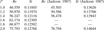
Data for the onset of this periodic shedding are provided in table 1. The value of
 $\mathit{Re}$
, as well as the value of
 $\mathit{St}$
at the onset of vortex shedding are provided, and compared to the values presented in Jackson (Reference Jackson1987). To find the value of
 $\mathit{Re}$
at the onset of vortex shedding, a series of simulations was run at increments of
 $\mathit{Re}$
of 1, and it was observed whether small perturbations grew or decayed. Growth was measured by monitoring the lift force coefficient
 $C_{\text{l}}=F_{L}/(1/2){\it\rho}U^{2}D$
on the body, where
 $F_{L}$
is the lift force per unit length, and
 ${\it\rho}$
is the fluid density. It was then assumed that the transition to periodic flow could be adequately modelled as a supercritical Hopf bifurcation (Provansal et al.
Reference Provansal, Mathis and Boyer1987; Dušek et al.
Reference Dušek, Le Gal and Fraunié1994; Thompson & Le Gal Reference Thompson and Le Gal2004), governed by the normal form equation
 $$\begin{eqnarray}\frac{\text{d}A}{\text{d}{\it\tau}}={\it\sigma}A+l_{c}|A|^{2}A,\end{eqnarray}$$
where
 $A$
is the amplitude of the oscillation (here taken as the amplitude of the lift force coefficient),
 ${\it\tau}$
is the non-dimensional time
 $tU/D$
where
 $t$
is time,
 ${\it\sigma}$
is the initial linear growth rate and
 $l_{c}$
is the Landau coefficient, which governs the saturation of the oscillation to a stable periodic state. This amplitude equation is often referred to as a Stuart–Landau model (Stuart Reference Stuart1958). By dividing by
 $A$
, (3.1) can be written as
 $$\begin{eqnarray}\frac{\text{d}\log (A)}{\text{d}{\it\tau}}={\it\sigma}+l_{c}|A|^{2}.\end{eqnarray}$$
The values of
 ${\it\sigma}$
and
 $l_{c}$
for a given simulation were then determined from a least-squares fit to the amplitude data of the form shown in (3.2). The values of
 ${\it\sigma}$
as a function of
 $\mathit{Re}$
were then fitted and the fit extrapolated to find the value of
 $\mathit{Re}$
where
 ${\it\sigma}=0$
.
Values of
 $\mathit{Re}$
and
 $\mathit{St}$
at the onset of periodic vortex shedding from the current study, compared with those of Jackson (Reference Jackson1987).

To find the frequency at the onset of vortex shedding, the frequency of the saturated state of the same set of simulations was measured, giving
 $\mathit{St}$
as a function of
 $\mathit{Re}$
. A curve was then fitted to these data, and the curve extrapolated to find the frequency at the value of
 $\mathit{Re}$
corresponding to
 ${\it\sigma}=0$
.
The comparison between the current results for the value of
 $\mathit{Re}$
at the onset of shedding and those of Jackson (Reference Jackson1987) is good, differing by a maximum of only 2.3 %. Whilst there is a larger discrepancy in the predicted frequencies, with differences of up to 15 %, it should be noted that the simulations of Jackson (Reference Jackson1987) were performed on a small domain, and so are affected by substantial blockage, artificially raising
 $\mathit{St}$
. Support for this comes from more recent studies (e.g. Thompson & Le Gal Reference Thompson and Le Gal2004; Sipp & Lebedev Reference Sipp and Lebedev2007) based on global stability analyses of the steady circular cylinder wake (
 ${\it\Gamma}=1$
). These studies report values of
 $\mathit{Re}_{c}=46.6$
and 46.4 at the onset of vortex shedding, and global mode frequencies of
 $\mathit{St}=0.11777$
and 0.1182, respectively. These values are very close to those found here, again with the small differences consistent with different domain blockage ratios, so providing some confidence in the results obtained for this study.
3.2. Variation of the growth rate of modes as a function of
 ${\it\Gamma}$
,
$\mathit{Re}=300$


In this section, results for a fixed
 $\mathit{Re}=300$
are presented as a function of
 ${\it\Gamma}$
. The value
 $\mathit{Re}=300$
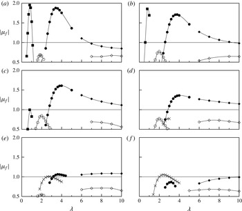
is chosen as both of modes A and B in the wake of a circular cylinder are known to be unstable at this value. Figure 1 presents
 $|{\it\mu}_{f}|$
as a function of spanwise wavelength
 ${\it\lambda}$
for six aspect ratios ranging from
 ${\it\Gamma}=1$
(a circular cylinder) to
 ${\it\Gamma}=2$
.
Floquet multiplier,
 ${\it\mu}_{f}$
, as a function of wavelength
 ${\it\lambda}$
, at
 $\mathit{Re}=300$
for: (a)
 ${\it\Gamma}=1.0$
(circle); (b)
 ${\it\Gamma}=1.2$
; (c)
 ${\it\Gamma}=1.4$
; (d)
 ${\it\Gamma}=1.6$
; (e)
 ${\it\Gamma}=1.8$
; ( f)
 ${\it\Gamma}=2.0$
. Each symbol designates a mode: mode A (●); mode B (▪); mode QP (○); mode
 $\widehat{\text{B}}$
(
 $\times$
); mode
 $\widehat{\text{A}}$
(♦); mode QPL (♢).

For wavelengths
 ${\it\lambda}\leqslant 5$
, the
 ${\it\Gamma}=1$
case shows the familiar picture for a circular cylinder; the flow is unstable to mode A over a band of wavelengths focused at
 ${\it\lambda}\simeq 3.5D$
and unstable to mode B for wavelengths of
 ${\it\lambda}\simeq 0.8D$
. Mode QP is found at
 ${\it\lambda}\simeq 1.8D$
, but it is not unstable at this
 $\mathit{Re}$
, achieving a maximum
 $|{\it\mu}_{f}|\simeq 0.7$
.
For longer wavelengths,
 $5<{\it\lambda}\leqslant 10$
, two other modes can be identified. The first of these modes, here named
 $\widehat{\text{A}}$
, appears to be a continuation of the mode A branch. It has the same spatiotemporal symmetries as mode A, and a purely real Floquet multiplier, yet has a slightly different spatial structure, as will be discussed in more detail later. The second of these modes is a quasi-periodic mode with a complex Floquet multiplier, and is here named mode QPL (for long-wavelength quasi-periodic). It has a maximum growth rate for
 ${\it\lambda}\simeq 9D$
.
With moderate increases in
 ${\it\Gamma}$
, this picture remains more or less the same. These same five modes are the only relevant modes up to
 ${\it\Gamma}=1.4$
. Increases in
 ${\it\Gamma}$
over this range see
 $|{\it\mu}_{f}|$
for mode A and mode B decrease. However,
 $|{\it\mu}_{f}|$
for mode QP increases, indicating an increase in growth rate. Despite this,
 $|{\it\mu}_{f}|$
for mode QP remains below
 $|{\it\mu}_{f}|=1$
, indicating it does not become unstable at this
 $\mathit{Re}$
. The maximum growth rate for mode
 $\widehat{\text{A}}$
changes little with
 ${\it\Gamma}$
, however the range of
 ${\it\lambda}$
over which it is unstable increases, extending to higher
 ${\it\lambda}$
with increasing
 ${\it\Gamma}$
. The growth of mode QPL remains largely untouched, with a maximum
 $|{\it\mu}_{f}|\simeq 0.8$
occurring at
 ${\it\lambda}\simeq 9D$
.
Further increases in
 ${\it\Gamma}$
up to
 ${\it\Gamma}=2$
show similar behaviour for modes A and B. Increases in
 ${\it\Gamma}$
see a reduction in
 $|{\it\mu}_{f}|$
. Mode B is stabilized (
 ${\it\mu}_{f}<1$
) at
 ${\it\Gamma}\simeq 1.4$
; mode A is stabilized at
 ${\it\Gamma}\simeq 1.8$
. The
 $|{\it\mu}_{f}|$
for mode QP also reduces, and this mode is not resolved for
 ${\it\Gamma}>1.8$
. A clear distinction between modes A and
 $\widehat{\text{A}}$
is seen for
 ${\it\Gamma}\geqslant 1.8$
; mode
 $\widehat{\text{A}}$
shows a clear local maximum in growth rate at
 ${\it\lambda}\simeq 8$
for
 ${\it\Gamma}=1.8$
, further delineating it from mode A. Mode QPL is again practically unchanged.
An important feature is that at
 ${\it\Gamma}=1.6$
, another mode with wavelengths around
 ${\it\lambda}=2.8$
, a purely real
 ${\it\mu}_{f}$
and spatiotemporal symmetry the same as for mode B is found. This mode, here named mode
 $\widehat{\text{B}}$
, sees
 $|{\it\mu}_{f}|$
increase with increasing
 ${\it\Gamma}$
. Mode
 $\widehat{\text{B}}$
is shown to be unstable for
 ${\it\Gamma}\geqslant 1.8$
.
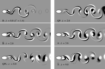
Images of the different modes at
 ${\it\Gamma}=1.8$
(except for mode B shown at
 ${\it\Gamma}=1.4$
) shown in order of increasing characteristic wavelength. The white and black contours represent spanwise perturbation vorticity over normalized levels of
 $\pm 0.1$
. The solid lines show contours of the base flow vorticity at levels
 $\pm 1$
. The structure of modes A, B and QP is very similar to their counterparts found in the wake of a circular cylinder. Mode
 $\widehat{\text{B}}$
has a distinct structure, but shares the same spatiotemporal symmetries as mode B. Mode
 $\widehat{\text{A}}$
has a similar structure to mode A in the two vortices closest to the body, but is distinct from the third vortex (circled with a dashed line) and further downstream. Note that modes QP and QPL are shown at an arbitrary phase as they have a complex
 ${\it\mu}_{f}$
.

Figure 2 shows images of each of the modes, all at
 $\mathit{Re}=300$
, in order of increasing characteristic wavelength
 ${\it\lambda}$
. All of the modes except mode B are shown at
 ${\it\Gamma}=1.8$
. Mode B is shown at
 ${\it\Gamma}=1.4$
as
 ${\it\mu}_{f}$
becomes so low at
 ${\it\Gamma}=1.8$
that the mode is no longer identifiable. The images show the spanwise perturbation vorticity as filled colour contours, overlaid with black contour lines showing the positions of the base flow vortex cores.
The structures of modes A, B and QP are the same as the structures found in the wake of a circular cylinder (Barkley & Henderson Reference Barkley and Henderson1996; Blackburn et al.
Reference Blackburn, Marques and Lopez2005). It should be noted that mode QP has a complex
 ${\it\mu}_{f}$
which introduces a second frequency, and as such the image shown in figure 2 is at an arbitrary phase.
Mode
 $\widehat{\text{B}}$
is shown to have a distinct structure. While the symmetry of this mode is the same as mode B, the mode shares many features with mode A, particularly the fact that it seems mainly focused in the wake vortex cores (although there is also significant amplitude in the braid shear layers that connect the wake vortices). However, mode
 $\widehat{\text{B}}$
has a finer structure on these vortex cores than mode A. An example of this is found by focusing on the negative vortex formed from the top of the body that is about to be shed into the wake immediately behind the body. Traversing across the centre of this approximately elliptical vortex along the short axis sees the sign of the perturbation vorticity change twice in mode
 $\widehat{\text{B}}$
(black–white–black); for mode A, it changes sign once (white–black). This is, of course, consistent with the shorter preferred wavelength of mode
 $\widehat{\text{B}}$
relative to mode A.
A mode found in the wake of elliptic leading-edge plates (Ryan et al.
Reference Ryan, Thompson and Hourigan2005), named mode
 $\text{B}^{\prime }$
, shares many of the characteristics of mode
 $\widehat{\text{B}}$
. It too has the same spatiotemporal symmetries as mode B, with a critical wavelength in the vicinity of
 ${\it\lambda}=2$
. The spatial structure of the two modes near the body is also quite similar in topology. These facts make it likely that mode
 $\widehat{\text{B}}$
found here and mode
 $\text{B}^{\prime }$
found in the wake of elliptic leading edge plates are due to the same physical mechanisms.
Exactly what these mechanisms are is not completely clear, and given the complicated structure of this mode it is possible that there are a number of cooperative mechanisms that contribute to its growth.
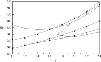
Plots of
 $\mathit{Re}_{c}$
, the value of
 $\mathit{Re}$
at marginal stability for all the modes as a function of
 ${\it\Gamma}$
. Points are measured values for mode A (●), mode B (▪), mode QP (○), mode
 $\widehat{\text{A}}$
(♦), mode
 $\widehat{\text{B}}$
(
 $\times$
). Lines are best fits to the measured values. The upper limit of instability for mode
 $\widehat{\text{B}}$
is marked with a dashed line as it is the result of extrapolation.

Mode
 $\widehat{\text{A}}$
has a structure very similar to mode A near the body. In the images shown in figure 2, the structure of modes A and
 $\widehat{\text{A}}$
are almost the same in the two vortices closest to the body. However, there is a distinct difference from the third vortex and further downstream. For instance, figure 2 shows mode A has one white lobe and one black lobe in the lower portion of the third vortex, and a white lobe in the upper portion of this vortex. Mode
 $\widehat{\text{A}}$
instead has a white lobe and a black lobe, both of which extend over the entire vortex (the vortices in question are circled with a dashed line in figure 2). Further downstream in the wake (but not shown here), mode
 $\widehat{\text{A}}$
displays a spanwise perturbation vorticity distribution strongly characteristic of elliptic instability. i.e. positive and negative lobes aligned at approximately 45
 $^{\circ }$
to the main axis of the base flow vortices. This is not as apparent in the downstream wake for the shorter wavelength mode A.
The structure of mode QPL is not dissimilar to mode QP. However, comparison of this mode’s structure is more difficult as it is dependent on the phase at which images are obtained. Over the parameter space tested, mode QPL was never seen to become unstable, and therefore further investigation of its structure does not seem warranted.
3.3. Variation of critical
$\mathit{Re}$
and wavelength for all modes as a function of
${\it\Gamma}$


Expanding on the results at a single
 $\mathit{Re}=300$
presented in § 3.2, this section presents the critical values of Reynolds number
 $\mathit{Re}_{c}$
and wavelength
 ${\it\lambda}_{c}$
for all four modes as a function of
 ${\it\Gamma}$
.
 $\mathit{Re}_{c}$
is the value of the Reynolds number at which a given mode is predicted to first become unstable (where
 $|{\it\mu}_{f}|$
first exceeds
 $|{\it\mu}_{f}|=1$
at some value of wavelength);
 ${\it\lambda}_{c}$
is the wavelength at which this occurs. For a given
 ${\it\Gamma}$
, calculations at a series of
 ${\it\lambda}$
in steps of 0.2 for a fixed
 $\mathit{Re}$
were run to find the maximum
 $|{\it\mu}_{f}|$
for a given mode, similar to the data presented in figure 1. The value of
 $\mathit{Re}$
was then incremented in steps of 20, finding a maximum
 $|{\it\mu}_{f}|$
and associated value of
 ${\it\lambda}$
for each
 $\mathit{Re}$
. This process was repeated until the maximum
 $|{\it\mu}_{f}|$
exceeded
 $|{\it\mu}_{f}|=1$
. The values of
 $\mathit{Re}_{c}$
and
 ${\it\lambda}_{c}$
were then found by quadratic interpolation of the surrounding values. Figures 3 and 4 present the results of these calculations. This same process was then performed for each aspect ratio.
The value of wavelength at marginal stability
 ${\it\lambda}_{c}$
for (a) mode A (●), mode B (▪), mode QP (○), mode
 $\widehat{\text{B}}$
(
 $\times$
) and (b) mode A (●), mode
 $\widehat{\text{A}}$
(♦) as a function of
 ${\it\Gamma}$
. Lines are best fits to the measured values.

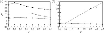
Figure 3 shows a number of features that warrant discussion. First,
 $\mathit{Re}_{c}$
is almost a linear function of
 ${\it\Gamma}$
for both modes A and B over the entire range tested. It also shows that, regardless of
 ${\it\Gamma}$
, the onset of mode A always precedes mode B.
This same figure shows that the relationship is more complicated for mode QP, as
 $\mathit{Re}_{c}$
first decreases with
 ${\it\Gamma}$
(for
 ${\it\Gamma}<1.5$
) and then increases with
 ${\it\Gamma}$
. Regardless,
 $\mathit{Re}_{c}$
for mode QP is always well beyond
 $\mathit{Re}_{c}$
for mode A, and so it is difficult to predict the influence this mode will have in a physical flow.
For
 ${\it\Gamma}>1.2$
, mode
 $\widehat{\text{A}}$
is found to be unstable. Below this value of
 ${\it\Gamma}$
, mode
 $\widehat{\text{A}}$
coalesces with mode A. Figure 3 shows that
 $\mathit{Re}_{c}$
is almost equal for modes A and
 $\widehat{\text{A}}$
at
 ${\it\Gamma}=1.2$
, and figure 4 shows that the critical wavelengths of the two modes are also the same at this
 ${\it\Gamma}$
, both providing evidence of the mode coalescence at this
 ${\it\Gamma}$
.
For
 ${\it\Gamma}>1.4$
, mode
 $\widehat{\text{A}}$
is clearly unstable at lower
 $\mathit{Re}$
than mode A. In fact, with respect to increasing
 $\mathit{Re}$
, mode
 $\widehat{\text{A}}$
is the first mode to become unstable until
 ${\it\Gamma}=1.9$
, where mode
 $\widehat{\text{B}}$
becomes the first to become unstable.
For
 ${\it\Gamma}>1.75$
, mode
 $\widehat{\text{B}}$
is found to be unstable. Unlike the other modes, an upper limit is found, such that mode
 $\widehat{\text{B}}$
is only unstable over a finite range of
 $\mathit{Re}$
. Of course, this is based on a linear analysis that fails to hold once the wake has undergone three-dimensional transition, changing the base flow state. In any case, mode
 $\widehat{\text{B}}$
is the leading instability mode, i.e. it is the first to become unstable with increasing
 $\mathit{Re}$
, for
 ${\it\Gamma}>1.9$
.
The prevalence of these two new modes,
 $\widehat{\text{A}}$
and
 $\widehat{\text{B}}$
, means that for moderate aspect ratios
 ${\it\Gamma}>1.5$
, the three-dimensional structure of the flow should be controlled by these modes, at least at
 $\mathit{Re}$
just above the first onset of three-dimensionality. This is further investigated in § 3.7.
The values of
 ${\it\lambda}_{c}$
presented in figure 4 show that the change in
 ${\it\Gamma}$
has the greatest impact on the wavelengths of modes A and
 $\widehat{\text{B}}$
. Figure 4(a) shows that the
 ${\it\lambda}_{c}$
for mode A first increases mildly, then decreases with increasing
 ${\it\Gamma}$
, falling to approximately
 ${\it\lambda}_{\text{c}}=3.5$
at
 ${\it\Gamma}=2$
, from
 ${\it\lambda}_{\text{c}}=4$
for the circular cylinder (
 ${\it\Gamma}=1$
). Once it is resolved,
 ${\it\lambda}_{c}$
for mode
 $\widehat{\text{B}}$
decreases with increasing
 ${\it\Gamma}$
. The value of
 ${\it\lambda}_{c}$
for mode B is essentially unchanged, and that for mode QP only varies slightly.
These changes naturally reflect the changes in the base flow. With increasing
 ${\it\Gamma}$
, the body becomes more streamlined, allowing the flow to remain attached for longer, reducing the wake width and the lateral spacing between vortices. The size and shape of these wake vortices will also be changed, becoming smaller. This is also caused by the reduced acceleration of the boundary-layer fluid as it advects over the ellipse prior to separation, leading to a lower vorticity flux into the wake. As outlined in § 1 (see also Leweke & Williamson Reference Leweke and Williamson1998; Thompson et al.
Reference Thompson, Leweke and Williamson2001), the mode A spanwise perturbation vorticity distribution shows strong characteristics associated with elliptic instability of shed near-wake vortices, and so it seems likely that its growth and preferred wavelength will be influenced by changes in the base flow (vorticity) configuration. The images presented in figure 2 show that mode
 $\widehat{\text{B}}$
also retains a high perturbation amplitude in the advecting vortex cores, and so it seems logical to assume that it too will be dependent on their configuration. On the other hand, mode B scales on the braid shear layers between vortices (Leweke & Williamson Reference Leweke and Williamson1998), and this scale apparently is not as susceptible to changes in the body aspect ratio as the wake vortex size and strength.
Figure 4(b) shows that
 ${\it\lambda}_{c}$
for mode
 $\widehat{\text{A}}$
increases almost linearly with increasing
 ${\it\Gamma}$
. It also shows that the
 ${\it\lambda}_{c}$
for mode
 $\widehat{\text{A}}$
can become very long, approaching
 ${\it\lambda}_{\text{c}}=28D$
at
 ${\it\Gamma}=2.4$
. However, the wavelength of highest growth for mode
 $\widehat{\text{A}}$
is a strong function of
 $\mathit{Re}$
. Therefore, as
 $\mathit{Re}$
is increased beyond
 $\mathit{Re}_{c}$
, the wavelength of mode
 $\widehat{\text{A}}$
typically becomes much shorter than
 ${\it\lambda}_{c}$
. This fact is further investigated and highlighted in § 3.6.
3.4. Behaviour of mode A in terms of elliptic instability theory
Leweke & Williamson (Reference Leweke and Williamson1998) employed the elliptic instability theory developed by Landman & Saffman (Reference Landman and Saffman1987) to the vortices in the wake of a circular cylinder. Even though the original theory was based on the instability of a single vortex with constant vorticity and a constant strain rate causing elliptical streamlines, Leweke & Williamson (Reference Leweke and Williamson1998) showed that the behaviour of the instability leading to mode A was at least consistent with this theory. Here, we take the same theory, and show that it predicts both the decrease in
 ${\it\lambda}_{c}$
with increasing
 ${\it\Gamma}$
, and the increase in
 $\mathit{Re}_{c}$
.
The theory developed by Landman & Saffman (Reference Landman and Saffman1987) predicts the growth rate of perturbations to an elliptic vortex, given the eccentricity and size of the vortex. The eccentricity
 ${\it\beta}={\it\epsilon}/(2|{\it\omega}|)$
, where
 ${\it\epsilon}$
is the strain rate and
 ${\it\omega}$
is the vorticity. For a two-dimensional flow, the local strain rate in Cartesian coordinates is given by
 $$\begin{eqnarray}{\it\epsilon}=\sqrt{\left|\frac{\partial u}{\partial x}\frac{\partial v}{\partial y}-\frac{1}{4}\left(\frac{\partial u}{\partial y}+\frac{\partial v}{\partial x}\right)^{2}\right|},\end{eqnarray}$$
which is the square root of the determinant of the symmetric part of the velocity gradient tensor.
For a purely elliptic vortex, both
 ${\it\omega}$
and
 ${\it\epsilon}$
are constant, however both can vary in space in a more complicated flow such as a bluff-body wake, and hence the local eccentricity
 ${\it\beta}$
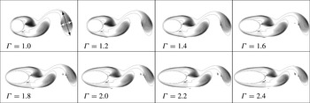
can also vary. Figure 5 shows images of the wake for a series of
 ${\it\Gamma}$
, at
 $\mathit{Re}_{c}$
for each case, where contours of vorticity are marked with solid lines, and values of the eccentricity are marked with greyscale contours. All of the images are shown at the instant where the lift force on the body is a maximum.
The wake at the instant of maximum lift force as a function of aspect ratio, at
 $\mathit{Re}_{c}$
for each case. Contours of non-dimensional vorticity at levels
 $\pm 1$
are marked with solid lines. Greyscale colour contours represent the local eccentricity
 ${\it\beta}$
at levels from 0 (black) to 1 (white). The white and black arrows on the example at
 ${\it\Gamma}=1$
show the measurement of the lengths of the minor and major axes
 $l_{minor}$
and
 $l_{major}$
of the wake vortices, respectively. The point of intersection of these lines indicates the point where
 ${\it\beta}$
of each vortex was measured. The vortices are shown to decrease in size with increasing
 ${\it\Gamma}$
, while the eccentricity at the centre of the vortices remains around a value of
 ${\it\beta}\simeq 0.6$
.

Figure 5 shows that regardless of
 ${\it\Gamma}$
(and the variation of
 $\mathit{Re}$
for each case), the eccentricity
 ${\it\beta}$
is basically constant with a value of around
 ${\it\beta}=0.6$
at the centre of the shed vortices. The eccentricity is not constant over the entire vortex but there is a region at the centre of each vortex where
 ${\it\beta}$
is not strongly varying.
The figure also shows that as
 ${\it\Gamma}$
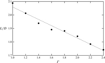
increases, the size of the vortices in the wake decreases. To quantify this decrease, the vortex furthest from the body in each of the images in Figure 5 was measured along its major and minor axes (where the boundary of the vortex was defined, reasonably arbitrarily, as the contour of
 $|{\it\omega}|=1$
), and a length scale
 $L=\sqrt{l_{major}^{2}+l_{minor}^{2}}$
defined, where
 $l_{major}$
and
 $l_{minor}$
are the lengths along the major and minor axes, respectively. This length scale
 $L$
is plotted as a function of
 ${\it\Gamma}$
in figure 6, and it is shown the
 $L$
decreases approximately linearly with
 ${\it\Gamma}$
.
Variation of the size of the wake vortices with
 ${\it\Gamma}$
. Here,
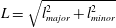 $L=\sqrt{l_{major}^{2}+l_{minor}^{2}}$
where
 $l_{major}$
and
 $l_{minor}$
are the lengths along the major and minor axes of the vortex as indicated in figure 5. Points are measurements, the dashed line is a linear fit.

Leweke & Williamson (Reference Leweke and Williamson1998) showed that the elliptic instability theory of Landman & Saffman (Reference Landman and Saffman1987) predicts wavelengths along the vortex core of
 $$\begin{eqnarray}{\it\lambda}=L\sqrt{\frac{2}{1-{\it\beta}}}\tan {\it\theta},\end{eqnarray}$$
where
 ${\it\theta}$
is the initial angle of incidence of the wavevector which results in the largest growth. For
 ${\it\beta}\leqslant 0.6$
, figure 3 of Landman & Saffman (Reference Landman and Saffman1987) shows that
 ${\it\theta}$
is basically a constant, and for
 ${\it\beta}=0.6$
(as measured at the centre of the vortices here)
 ${\it\theta}\simeq 7{\rm\pi}/24\simeq 53^{\circ }$
.
If both
 ${\it\beta}$
and
 ${\it\theta}$
are constant, (3.4) shows that
 ${\it\lambda}$
is proportional to
 $L$
. Figure 6 shows that
 $L$
decreases linearly with
 ${\it\Gamma}$
, so it is expected that
 ${\it\lambda}$
should also decrease linearly. Figure 4 shows that this is indeed the case, at least over the range
 $1.2<{\it\Gamma}<2.4$
.
Concerning the critical Reynolds number, Landman & Saffman (Reference Landman and Saffman1987) showed that the growth rate of the elliptic instability is made up of two components; an inviscid growth rate
 ${\it\sigma}_{i}$
and a viscous decay rate (effectively a negative growth rate)
 ${\it\sigma}_{v}$
. When time is non-dimensionalized by
 $D/U$
, this viscous decay rate is given by
 $$\begin{eqnarray}{\it\sigma}_{v}=\frac{1}{\mathit{Re}}\frac{2{\rm\pi}}{{\it\lambda}}\frac{1-{\it\beta}\cos ^{2}{\it\theta}}{(1-{\it\beta})\cos ^{2}{\it\theta}}.\end{eqnarray}$$
At neutral stability, the overall growth rate is zero, such that
 ${\it\sigma}_{i}={\it\sigma}_{v}$
. It therefore also seems reasonable to assume that at neutral stability, the viscous decay rate is constant. If
 ${\it\sigma}_{v}$
is constant, and since both
 ${\it\beta}$
and
 ${\it\theta}$
have been shown to be constant, then from (3.5)
 $\mathit{Re}_{c}\propto {\it\lambda}^{-2}\propto (1-{\it\zeta}{\it\Gamma})^{-2}$
, where
 ${\it\zeta}$
is a constant. It is therefore expected that
 $\mathit{Re}_{c}$
should increase with
 ${\it\Gamma}$
, which seems consistent with the trend of
 $\mathit{Re}_{c}$
observed and plotted in figure 3.
The fact that the elliptic instability theory presented by Landman & Saffman (Reference Landman and Saffman1987) seems to at least be consistent with the trends in
 ${\it\lambda}_{c}$
and
 $\mathit{Re}_{c}$
observed during the Floquet stability analysis is further evidence that an elliptic instability plays a role in the development of mode A.
3.5. Calculation of the upper limit of instability for mode
$\widehat{\text{B}}$

The upper limit of instability for mode
 $\widehat{\text{B}}$
is difficult to compute. figure 3 shows that this upper limit occurs at much higher
 $\mathit{Re}$
than the
 $\mathit{Re}_{c}$
of mode A. The Floquet multiplier of mode A can therefore be quite large, while by definition the Floquet multiplier for mode
 $\widehat{\text{B}}$
at the upper limit is
 $|{\it\mu}_{f}|=1$
. This means that it can become very difficult to isolate mode
 $\widehat{\text{B}}$
when searching for leading eigenvalues and eigenvectors using a Krylov subspace-based method such as that employed here. Of course, if the flow is already three-dimensional through amplification and saturation of other three-dimensional modes, as is the case here, the upper limit of positive growth for mode
 $\widehat{\text{B}}$
will not have strong physical relevance, since the base flow for the stability analysis is no longer two-dimensional.
To estimate the location of this upper limit, the maximum Floquet multipliers have been calculated for mode
 $\widehat{\text{B}}$
at lower values of
 $\mathit{Re}$
, and the trend extrapolated to find where
 $|{\it\mu}_{f}|=1$
. The data for aspect ratios
 $1.8\leqslant {\it\Gamma}\leqslant 2.4$
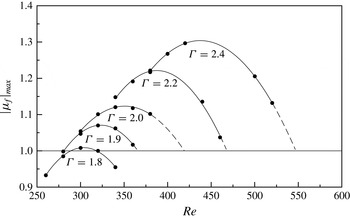
are presented in figure 7. The figure plots the maximum value of
 $|{\it\mu}_{f}|$
for all wavelengths for mode
 $\widehat{\text{B}}$
as a function of
 $\mathit{Re}$
. For all values of
 ${\it\Gamma}$
, it is clear that there is a turning point, and that beyond this turning point the maximum
 $|{\it\mu}_{f}|$
decreases with further increases in
 $\mathit{Re}$
. For the lower values of
 ${\it\Gamma}$
, e.g.
 ${\it\Gamma}=1.8$
, it is possible to resolve mode
 $\widehat{\text{B}}$
beyond the upper limit, and the value of
 $\mathit{Re}$
at this upper limit can be found from interpolation. However, for higher values of
 ${\it\Gamma}$
this upper limit needs to be estimated by extrapolating the data.
The magnitude of the maximum Floquet multiplier for mode
 $\widehat{\text{B}}$
as a function of
 $\mathit{Re}$
, for different
 ${\it\Gamma}$
. Dashed lines show extrapolation to
 $|{\it\mu}_{f}|=1$
for
 $\mathit{Re}$
where mode
 $\widehat{\text{B}}$
cannot be resolved due to the much higher Floquet multiplier of mode A.

3.6. The relationship between modes
$\text{A}$
and
$\widehat{\text{A}}$


As highlighted in § 3.3, modes A and
 $\widehat{\text{A}}$
appear to coalesce for
 ${\it\Gamma}<1.2$
. Figure 2 shows that they are quite similar in spatial structure, especially in the vortices that are close to the body. Only in the vortices further downstream do they differ enough to be identified as distinct modes. As such, care needs to be taken when performing the stability analysis to ensure the two modes are successfully distinguished.
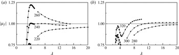
Figure 8 shows the magnitude of the Floquet multiplier
 $|{\it\mu}_{f}|$
as a function of wavelength
 ${\it\lambda}$
for modes A and
 $\widehat{\text{A}}$
at
 ${\it\Gamma}=1.4$
and
 ${\it\Gamma}=2.0$
, at a series of values of
 $\mathit{Re}$
. The change in character of the curves with increasing
 $\mathit{Re}$
for the
 ${\it\Gamma}=1.4$
case is clear.
At
 $\mathit{Re}=220$
, modes A and
 $\widehat{\text{A}}$
have clearly defined ‘branches’. Mode A shows a peak in
 $|{\it\mu}_{f}|$
at
 ${\it\lambda}\simeq 3.5$
, and
 $|{\it\mu}_{f}|$
for mode
 $\widehat{\text{A}}$
increases with increasing
 ${\it\lambda}$
beyond this.
At
 $\mathit{Re}=240$
, modes A and
 $\widehat{\text{A}}$
have clearly defined branches, and there is a peak for
 $|{\it\mu}_{f}|$
for mode
 $\widehat{\text{A}}$
around
 ${\it\lambda}=7$
.
By
 $\mathit{Re}=260$
, the distinction between the branches of mode A and
 $\widehat{\text{A}}$
disappears, and there seems to be a single curve of
 $|{\it\mu}_{f}|$
as a function of
 ${\it\lambda}$
. Modes A and
 $\widehat{\text{A}}$
in this case can only be (weakly) distinguished by inspecting the perturbation fields similar to those presented in figure 2. This also means that, like the case at
 $\mathit{Re}=220$
, there is no value of
 ${\it\lambda}$
at which a peak in
 $|{\it\mu}_{f}|$
occurs.
The data for
 ${\it\Gamma}=2$
presented in figure 8(b) show similar issues. While the branches of mode A and
 $\widehat{\text{A}}$
are clearly defined for all of the values of
 $\mathit{Re}$
shown, lower values of
 $\mathit{Re}$
result in curves that do not have a clearly defined peak for mode
 $\widehat{\text{A}}$
.
Magnitude of the Floquet multiplier
 $|{\it\mu}_{f}|$
as a function of wavelength
 ${\it\lambda}$
for (a)
 ${\it\Gamma}=1.4$
and (b)
 ${\it\Gamma}=2.0$
. Symbols mark mode A (●) and mode
 $\widehat{\text{A}}$
(♦). The
 $\mathit{Re}$
for each curve is indicated on the figure. For
 ${\it\Gamma}=1.4$
shown in (a), a peak in the curves for mode
 $\widehat{\text{A}}$
is difficult to discern and the mode A and
 $\widehat{\text{A}}$
curves appear to merge at higher
 $\mathit{Re}$
. For
 ${\it\Gamma}=2.0$
, the two modes are more clearly delineated.

Implicitly, figure 8 also shows how the characteristic wavelength of mode
 $\widehat{\text{A}}$
varies with
 $\mathit{Re}$
. It is shown for both values of
 ${\it\Gamma}$
that the maximum value of growth changes from occurring at very large wavelengths at lower
 $\mathit{Re}$
, to relatively small wavelengths at higher
 $\mathit{Re}$
. In particular, this means that the wavelength of the mode which is actually observed in a flow at a value of
 $\mathit{Re}$
beyond
 $\mathit{Re}_{c}$
may be markedly shorter that
 ${\it\lambda}_{c}$
. This point is shown explicitly in the three-dimensional simulations presented in § 3.7.
The usual method of finding the critical values
 $\mathit{Re}_{c}$
and
 ${\it\lambda}_{c}$
involves finding
 $|{\it\mu}_{f}|_{max}$
at specified values of
 ${\it\lambda}$
as a function of
 $\mathit{Re}$
, and then interpolating for the value of
 $\mathit{Re}$
where
 $|{\it\mu}_{f}|_{max}=1$
. As
 $|{\it\mu}_{f}|_{max}$
is not defined with a distinct peak, applying this method is more difficult for mode
 $\widehat{\text{A}}$
. Instead, for a given value of
 ${\it\lambda}$
, the value of
 $\mathit{Re}$
where
 $|{\it\mu}_{f}|=1$
is found via interpolation. These values are then plotted as a function of
 ${\it\lambda}$
. The minimum value of
 $\mathit{Re}$
where
 $|{\it\mu}_{f}|=1$
, and the corresponding value of
 ${\it\lambda}$
, are identified, and these are
 $\mathit{Re}_{c}$
and
 ${\it\lambda}_{c}$
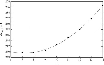
, respectively. An example of the data from this process, for
 ${\it\Gamma}=1.4$
, is shown in figure 9.
Plot of
 $\mathit{Re}$
where
 $|{\it\mu}_{f}|=1$
for mode
 $\widehat{\text{A}}$
,
 ${\it\Gamma}=1.4$
. Points represent values interpolated from the data (such as that presented in figure 8), the solid line represents a quadratic fit to these values. The minimum of this curve gives the critical values of
 $\mathit{Re}$
and
 ${\it\lambda}$
.

The exact physical mechanism that leads to instability of mode
 $\widehat{\text{A}}$
is not clear. Due to its structural similarity to mode A near the body, it seems fair to assume that the mechanisms that cause mode A (which is at least partially due to an elliptic instability) also play a role in mode
 $\widehat{\text{A}}$
. However, the wavelength selection and modification in the wake away from the body is possibly due to a number of cooperative mechanisms, and at this stage any description of them is only speculative.
3.7. Three-dimensional simulations confirming the existence of modes
$\widehat{\text{A}}$
and
$\widehat{\text{B}}$


The data from the stability analysis, particularly those shown in figure 3, indicate that for higher values of
 ${\it\Gamma}$
, the two new modes
 $\widehat{\text{B}}$
and
 $\widehat{\text{A}}$
should be the first modes observed with increasing
 $\mathit{Re}$
.
Full three-dimensional simulations at
 ${\it\Gamma}=2$
have been conducted to investigate this at two values of the Reynolds number:
 $\mathit{Re}=300$
and
 $\mathit{Re}=350$
. These simulations are based on extending the two-dimensional spectral-element code and meshes into the spanwise direction using a Fourier series representation as described by Karniadakis & Triantafyllou (Reference Karniadakis and Triantafyllou1992) and Thompson et al. (Reference Thompson, Hourigan and Sheridan1996). The simulations were initialized using the two-dimensional periodic base flow, with low-level random noise (amplitude
 $O(10^{-4})$
) added to initiate the development of the three-dimensional flow. In both simulations, 128 Fourier planes were used to represent the flow in the spanwise direction.
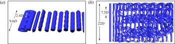
Visualizations of the flow using isosurfaces of the
 ${\it\lambda}_{2}$
criterion defined by Jeong & Hussain (Reference Jeong and Hussain1995) for vortex identification are shown in figure 10.
Visualization of the flow calculated from three-dimensional direct numerical simulation at (a)
 ${\it\Gamma}=2$
,
 $\mathit{Re}=300$
and (b)
 ${\it\Gamma}=2$
,
 $\mathit{Re}=350$
. Isosurfaces show the
 ${\it\lambda}_{2}=-0.001$
criterion from Jeong & Hussain (Reference Jeong and Hussain1995). The total length of the domain, and one wavelength of the dominant mode, are marked for both cases.

The image in figure 10(a) corresponds to
 $\mathit{Re}=300$
, which figure 3 indicates should result in both modes
 $\widehat{\text{A}}$
and
 $\widehat{\text{B}}$
being unstable. However, figure 4 indicates that
 ${\it\lambda}_{c}$
for mode
 $\widehat{\text{A}}$
for
 $\mathit{Re}=300$
occurs at
 ${\it\lambda}_{\text{c}}\simeq 20$
. Therefore, to isolate the modes, the domain for this simulation was restricted to
 $9.6D$
so that only mode
 $\widehat{\text{B}}$
could exist within the domain and thus grow. The spanwise domain size was chosen to allow four mode
 $\widehat{\text{B}}$
wavelength to fit within the domain. The image shows that indeed a mode with a wavelength
 ${\it\lambda}=2.4D$
grows, which is very close to the wavelength predicted for mode
 $\widehat{\text{B}}$
by the stability analysis as shown in figure 4.
At this Reynolds number, the saturated state of mode
 $\widehat{\text{B}}$
shown in figure 10(a) shows that it manifests as a relatively weak modulation of the forming vortices. This modulation attenuates as the vortices progress downstream.
The simulation at
 $\mathit{Re}=350$
was conducted on a longer domain of
 $22D$
. The larger domain was used in this case to allow modes with a wider range of wavelengths to develop, and to observe which modes would naturally dominate the saturated state. Figure 3 shows that modes A,
 $\widehat{\text{B}}$
and
 $\widehat{\text{A}}$
are all linearly unstable at this Reynolds number. As the flow evolves towards saturation, figure 10(b) shows the emergence of a mode with a wavelength
 ${\it\lambda}\simeq 7.5D$
. This is mode
 $\widehat{\text{A}}$
. The wavelength of the mode in the three-dimensional simulation (
 ${\it\lambda}=7.5D$
) is much shorter than the critical wavelength for mode
 $\widehat{\text{A}}$
(
 ${\it\lambda}_{\text{c}}=20D$
). However, mode
 $\widehat{\text{A}}$
first becomes critical at
 $\mathit{Re}=290$
, and the three-dimensional simulation was conducted at
 $\mathit{Re}=350$
. Stability calculations beyond the critical the critical
 $\mathit{Re}$
show that the fastest-growing wavelength of mode
 $\widehat{\text{A}}$
rapidly reduces with increasing
 $\mathit{Re}$
. In fact, stability calculations at
 $\mathit{Re}=350$
predict a wavelength of around
 $7.5D$
, similar to that measured in the three-dimensional simulation. The image shows that mode
 $\widehat{\text{A}}$
results in an initial sinuous modulation of the wake vortices, and the rapid development of a complicated series of streamwise vortices at a distance of only a few diameters. Further downstream again, there appears to be complicated vortex pairing and nonlinear interactions occurring.
Interestingly, even though mode
 $\widehat{\text{B}}$
is unstable first with respect to increasing
 $\mathit{Re}$
, it appears that the wake is dominated by a wavelength attributable to mode
 $\widehat{\text{A}}$
at
 $\mathit{Re}=350$
. This is not entirely inconsistent with the predictions from the stability analysis. Figure 7 shows that the Floquet multiplier of mode
 $\widehat{\text{B}}$
never reaches large values, and actually begins to decrease with further increases in
 $\mathit{Re}$
. Therefore, beyond the initial transition the Floquet multiplier of mode
 $\widehat{\text{A}}$
can exceed that of mode
 $\widehat{\text{B}}$
and dominate the wake.
4. Concluding remarks
Floquet stability analysis of the flow past an elliptical cylinder has shown that for aspect ratios
 ${\it\Gamma}<1.4$
, the three-dimensional transition sequence (mode A, B, QP) is the same as for the circular cylinder, albeit occurring at higher
 $\mathit{Re}$
with increasing
 ${\it\Gamma}$
. At
 ${\it\Gamma}>1.2$
, the mode A stability branch effectively splits into two segments with two distinct peaks in the Floquet multiplier curves. In fact, the longer-wavelength branch gives mode
 $\widehat{\text{A}}$
, which is the most unstable mode for
 $1.4D\lesssim {\it\lambda}\lesssim 1.9D$
. For
 ${\it\Gamma}>1.75$
, another new mode, named mode
 $\widehat{\text{B}}$
, is found. This mode has the same spatiotemporal symmetry as mode B, but maintains high amplitude in the advecting wake vortex cores, similar to that found for mode A. In terms of structure, mode
 $\widehat{\text{B}}$
has an apparent higher radial wavenumber on the wake vortices than mode A, consistent with its shorter preferred wavelength. A similar mode called mode
 $\text{B}^{\prime }$
was previously found for elongated cylinders with elliptical noses and a flat base (Ryan et al.
Reference Ryan, Thompson and Hourigan2005). Here, this mode is the first occurring for
 ${\it\Gamma}\gtrsim 1.9D$
.
Based on the stability analysis at a given aspect ratio, at higher Reynolds numbers the mode A and
 $\widehat{\text{A}}$
Floquet branches merge, with the mode A Floquet multiplier regaining dominance. In addition, the maximum value of the mode
 $\widehat{\text{B}}$
multiplier is limited and indeed decreases as the Reynolds number is further increased beyond some point. Thus, beyond the initial transition, it is not clear how strong the influence of the two new modes will be on the fully developed wake state. But in any case, while the circular cylinder transition sequence is maintained for aspect ratios close to unity, further away, this scenario is altered considerably.
Acknowledgements
The authors would like to acknowledge the financial support of the Australian Research Council (ARC) through grant number DP110102141 under the Discovery program, and the Centre National de la Recherche Scientifique (CNRS) through grant number CNRS/PICS 49586. J.S.L. would like to acknowledge the financial support of the ARC through an Australian Postdoctoral Fellowship.