2 Characterization of velocity gradients and local streamline topology

Velocity gradients play a critical role in scalar mixing. In this section, we identify three distinct characteristics of the velocity-gradient tensor – magnitude, topology and normalized dilatation level. The velocity-gradient tensor is given by

(2.1) $$\begin{eqnarray}\unicode[STIX]{x1D608}_{ij}\equiv \frac{\partial V_{j}}{\partial x_{i}},\end{eqnarray}$$

where $V_{i}$ and $x_{i}$ denote velocity and spatial coordinates respectively. The symmetric and anti-symmetric parts of the $\unicode[STIX]{x1D608}_{ij}$ tensor represent the strain-rate $(\unicode[STIX]{x1D61A}_{ij})$ and the rotation-rate tensors $\unicode[STIX]{x1D61E}_{ij}$ :

(2.2a,b ) $$\begin{eqnarray}\unicode[STIX]{x1D61A}_{ij}\equiv \frac{\unicode[STIX]{x1D608}_{ij}+\unicode[STIX]{x1D608}_{ji}}{2},\quad \unicode[STIX]{x1D61E}_{ij}\equiv \frac{\unicode[STIX]{x1D608}_{ij}-\unicode[STIX]{x1D608}_{ji}}{2}.\end{eqnarray}$$

The trace of the velocity-gradient tensor $(\unicode[STIX]{x1D608}_{ii})$ represents the rate of change in volume or the dilatation rate of the local fluid element. A positive/negative/zero value implies an expanding/contracting/volume-preserving fluid element.

The velocity-gradient tensor can be expressed in terms of its normalized form $(\unicode[STIX]{x1D622}_{ij})$ and its magnitude $({\it\epsilon})$ as

(2.3) $$\begin{eqnarray}\unicode[STIX]{x1D608}_{ij}\equiv {\it\epsilon}\unicode[STIX]{x1D622}_{ij},\end{eqnarray}$$

where

(2.4) $$\begin{eqnarray}{\it\epsilon}=\sqrt{\unicode[STIX]{x1D608}_{ij}\unicode[STIX]{x1D608}_{ij}}.\end{eqnarray}$$

The magnitude of the tensor is represented by the scalar ${\it\epsilon}$ , whereas the topological properties are resident in $\unicode[STIX]{x1D622}_{ij}$ . Clearly, the normalization ensures that each component of $\unicode[STIX]{x1D622}_{ij}$ remains bounded within the interval $[-1,1]$ . Based on $\unicode[STIX]{x1D622}_{ij}$ , we can define normalized strain-rate $(\unicode[STIX]{x1D634}_{ij})$ and normalized rotation-rate $(\unicode[STIX]{x1D638}_{ij})$ tensors as

(2.5a,b ) $$\begin{eqnarray}\unicode[STIX]{x1D634}_{ij}\equiv \frac{\unicode[STIX]{x1D622}_{ij}+\unicode[STIX]{x1D622}_{ji}}{2},\quad \unicode[STIX]{x1D638}_{ij}\equiv \frac{\unicode[STIX]{x1D622}_{ij}-\unicode[STIX]{x1D622}_{ji}}{2}.\end{eqnarray}$$

Similarly, we can define a normalized form of the dilatation rate:

(2.6) $$\begin{eqnarray}\unicode[STIX]{x1D622}_{ii}=\frac{\unicode[STIX]{x1D608}_{ii}}{{\it\epsilon}}~(\equiv {\it\Pi}).\end{eqnarray}$$

The normalized dilatation rate is mathematically bounded between $-\sqrt{3}$ and $\sqrt{3}$ .

In the principal coordinate system of $\unicode[STIX]{x1D634}_{ij}$ , $\unicode[STIX]{x1D622}_{ij}$ can be expressed as

(2.7) $$\begin{eqnarray}\unicode[STIX]{x1D656}=\left[\begin{array}{@{}ccc@{}}{\it\alpha} & 0 & 0\\ 0 & {\it\beta} & 0\\ 0 & 0 & {\it\gamma}\end{array}\right]+\frac{1}{2}\left[\begin{array}{@{}ccc@{}}0 & -{\it\omega}_{{\it\gamma}} & {\it\omega}_{{\it\beta}}\\ {\it\omega}_{{\it\gamma}} & 0 & -{\it\omega}_{{\it\alpha}}\\ -{\it\omega}_{{\it\beta}} & {\it\omega}_{{\it\alpha}} & 0\end{array}\right]+{\it\Pi}\frac{{\it\delta}_{ij}}{3},\end{eqnarray}$$

where ${\it\alpha}$ , ${\it\beta}$ and ${\it\gamma}$ represent the eigenvalues of the anisotropic strain rate $(\unicode[STIX]{x1D634}_{ij}^{a}\equiv \unicode[STIX]{x1D634}_{ij}-{\it\Pi}({\it\delta}_{ij}/3))$ , with ${\it\alpha}\geqslant {\it\beta}\geqslant {\it\gamma}$ , ${\it\Pi}$ is the trace of the strain-rate tensor ( $\unicode[STIX]{x1D634}_{ij}$ ), and ${\it\omega}_{{\it\alpha}}$ , ${\it\omega}_{{\it\beta}}$ and ${\it\omega}_{{\it\gamma}}$ are the components of the vorticity vector ${\bf\omega}$ along the three eigendirections of $\boldsymbol{s}$ .

The local shape or topology of the streamlines depends upon the nature of the eigenvalues of the velocity-gradient tensor, which in turn can be inferred from a knowledge of the three invariants of $\unicode[STIX]{x1D622}_{ij}$ (Cantwell, Lewis & Chen Reference Cantwell, Lewis and Chen1989; Chen, Cantwell & Mansour Reference Chen, Cantwell and Mansour1989; Chen et al. Reference Chen, Chong, Soria, Sondergaard, Perry, Rogers, Moser and Cantwell1990; Chong, Perry & Cantwell Reference Chong, Perry and Cantwell1990; Cantwell Reference Cantwell1992, Reference Cantwell1993; Soria et al. Reference Soria, Sondergaard, Cantwell, Chong and Perry1994). These invariants are defined as

(2.8) $$\begin{eqnarray}\left.\begin{array}{@{}c@{}}\displaystyle p=-\unicode[STIX]{x1D622}_{ii},\quad q={\textstyle \frac{1}{2}}(p^{2}-\unicode[STIX]{x1D634}_{ij}\unicode[STIX]{x1D634}_{ji}-\unicode[STIX]{x1D638}_{ij}\unicode[STIX]{x1D638}_{ji})\quad \text{and}\\ \displaystyle r={\textstyle \frac{1}{3}}(-p^{3}+3pq-\unicode[STIX]{x1D634}_{ij}\unicode[STIX]{x1D634}_{jk}\unicode[STIX]{x1D634}_{ki}-3\unicode[STIX]{x1D638}_{ij}\unicode[STIX]{x1D638}_{jk}\unicode[STIX]{x1D634}_{ki}).\end{array}\right\}\end{eqnarray}$$

2.1 Flow-field topology

The topology represents the local instantaneous streamline pattern around an infinitesimal fluid element observed with respect to a reference frame which is non-rotating but translating with the fluid element. With respect to such a reference frame, the centre of the local fluid element is a critical point (Perry & Chong Reference Perry and Chong1987; Chong et al. Reference Chong, Perry and Cantwell1990). The observed streamline pattern then depends on the nature of the eigenvalues of the velocity-gradient tensor $(\unicode[STIX]{x1D608}_{ij})$ . In the recent past, several topology-based studies have been reported for a variety of flow fields, leading to an improved understanding of turbulence: Hunt, Wray & Moin (Reference Hunt, Wray and Moin1988), Cantwell et al. (Reference Cantwell, Lewis and Chen1989), Chen et al. (Reference Chen, Chong, Soria, Sondergaard, Perry, Rogers, Moser and Cantwell1990), Boratav & Pelz (Reference Boratav and Pelz1995), Blackburn, Mansour & Cantwell (Reference Blackburn, Mansour and Cantwell1996), Chacin, Cantwell & Kline (Reference Chacin, Cantwell and Kline1996), Soria, Ooi & Chong (Reference Soria, Ooi and Chong1997), Maekawa, Hiyama & Matsuo (Reference Maekawa, Hiyama and Matsuo1999), Pirozzoli & Grasso (Reference Pirozzoli and Grasso2004), da Silva & Pereira (Reference da Silva and Pereira2008), Suman & Girimaji (Reference Suman and Girimaji2010), Wang & Lu (Reference Wang and Lu2012), Chu & Lu (Reference Chu and Lu2013), Boschung et al. (Reference Boschung, Schaefer, Peters and Meneveau2014), Cifuentes et al. (Reference Cifuentes, Dopazo, Martin and Jimenez2014), Vaghefi & Madnia (Reference Vaghefi and Madnia2015).

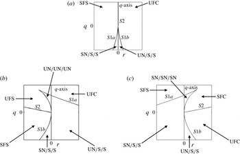
The reader is referred to Chong et al. (Reference Chong, Perry and Cantwell1990) and Suman & Girimaji (Reference Suman and Girimaji2010) for a detailed description of various topologies in a compressible flow field. Here, we provide just a brief summary. In figure 1, we show three representative $q{-}r$ planes at $p=0$ , $p<0$ and $p>0$ . On each of these planes, four curves can be seen: $S1a$ , $S1b$ , $S2$ and the $q$ -axis. The pair of curves $S1a$ and $S1b$ divide the $q{-}r$ plane into regions where the three eigenvalues of $\unicode[STIX]{x1D622}_{ij}$ are either (a) all real or (b) one real and two complex conjugates. The straight line $S2$ represents purely imaginary eigenvalues and further splits the region of complex eigenvalues into two. On the $p=0$ plane, $S2$ is coincident with the $q$ -axis, and $S1a$ and $S1b$ are symmetric about the $q$ -axis, dividing the $q{-}r$ plane into four regions. However, on a $p<0$ or $p>0$ plane this symmetry is lost, and $S2$ is no longer coincident with the $q$ -axis. 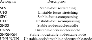This leads to six distinctly identifiable regions on $p<0$ and $p>0$ planes. Each of these regions corresponds to a particular topology (marked on figure 1). A description of the various acronyms is provided in table 1.

Figure 1.

Regions on (a) the $p=0$ ( $\unicode[STIX]{x1D622}_{ii}=0$ ) plane, (b) a negative $p$ ( $\unicode[STIX]{x1D622}_{ii}>0$ ) plane and (c) a positive $p$ ( $\unicode[STIX]{x1D622}_{ii}<0$ ) plane, and the corresponding topologies. A description of the acronyms is provided in table 1.

Table 1.

Description of acronyms.

It should be noted that the qualifier stable implies that the corresponding solution trajectories or the local streamlines are directed towards the centre of the fluid element (critical point). Similarly, unstable implies that the local streamlines are directed away from the centre of the fluid element. It should be noted that SFC, UFC, UFS and SFS are topologies with a focus (focal topologies) and are associated with complex eigenvalues of the velocity-gradient tensor. On the other hand, UNSS, SNSS, UN/UN/UN and SN/SN/SN are topologies associated with three real eigenvalues of the velocity-gradient tensor (non-focal topologies).

3 Scalar dissipation analysis

In this section, we examine the scalar dissipation evolution equation and highlight the role of the velocity field in scalar mixing. We start with the mass, momentum and energy conservation equations along with the state equation of a calorically perfect gas:

(3.1) $$\begin{eqnarray}\frac{\partial {\it\rho}}{\partial t}+V_{k}\frac{\partial {\it\rho}}{\partial x_{k}}=-{\it\rho}\frac{\partial V_{k}}{\partial x_{k}},\end{eqnarray}$$

(3.2) $$\begin{eqnarray}\frac{\partial V_{i}}{\partial t}+V_{k}\frac{\partial V_{i}}{\partial x_{k}}=-\frac{1}{{\it\rho}}\frac{\partial p}{\partial x_{i}}+\frac{\partial {\it\sigma}_{ik}}{{\it\rho}\partial x_{k}},\end{eqnarray}$$

(3.3) $$\begin{eqnarray}\frac{\partial T}{\partial t}+V_{k}\frac{\partial T}{\partial x_{k}}=-T(n-1)\frac{\partial V_{i}}{\partial x_{i}}-\frac{n-1}{{\it\rho}R}\frac{\partial q_{k}}{\partial x_{k}}+\frac{n-1}{{\it\rho}R}\frac{\partial }{\partial x_{j}}\left(V_{i}{\it\sigma}_{ji}\right).\end{eqnarray}$$

Here, $V_{i}$ , ${\it\rho}$ , $p$ , $T$ , $R$ , ${\it\sigma}_{ik}$ , $q_{k}$ and $n$ denote velocity, density, pressure, temperature, gas constant, stress tensor, heat flux and ratio of specific heat values respectively. The three thermodynamic variables, ${\it\rho}$ , $T$ and $p$ , are related through the state equation:

(3.4) $$\begin{eqnarray}p={\it\rho}RT.\end{eqnarray}$$

The viscous stress tensor ( ${\it\sigma}_{ij}$ ) and the heat flux vector ( $q_{k}$ ) obey the following constitutive relationships:

(3.5a,b ) $$\begin{eqnarray}{\it\sigma}_{ij}\equiv {\it\mu}\left(\frac{\partial V_{i}}{\partial x_{j}}+\frac{\partial V_{j}}{\partial x_{i}}\right)+{\it\delta}_{ij}{\it\lambda}\frac{\partial V_{k}}{\partial x_{k}},\quad q_{k}\equiv -K\frac{\partial T}{\partial x_{k}},\end{eqnarray}$$

where ${\it\mu}$ , ${\it\lambda}$ and $K$ denote the first and second coefficients of viscosity and the thermal conductivity respectively. It should be noted that ${\it\lambda}$ is taken as $-(2{\it\mu}/3)$ . Next, we consider a resident passive scalar ( ${\it\theta}$ ) that evolves according to the following equation:

(3.6) $$\begin{eqnarray}\frac{\partial \left({\it\rho}{\it\theta}\right)}{\partial t}+\frac{\partial ({\it\rho}V_{k}{\it\theta})}{\partial x_{k}}=\frac{\partial }{\partial x_{k}}\left(D\frac{\partial {\it\theta}}{\partial x_{k}}\right),\end{eqnarray}$$

where $D$ is the scalar diffusivity, which is assumed to be a constant.

Compressible turbulent flow fields are decomposed into their density-averaged (Favre-averaged) values and the residual Favre fluctuations. For a flow variable ${\it\psi}$ , the Favre-averaged value ( $\widetilde{{\it\psi}}$ ) and Favre fluctuation ( ${\it\psi}^{\prime \prime }$ ) are defined as

(3.7a,b ) $$\begin{eqnarray}\widetilde{{\it\psi}}=\frac{\left\langle {\it\rho}{\it\psi}\right\rangle }{\left\langle {\it\rho}\right\rangle }\quad \text{and}\quad {\it\psi}^{\prime \prime }={\it\psi}-\widetilde{{\it\psi}},\end{eqnarray}$$

where $\langle \cdot \rangle$ denotes Reynolds averaging.

The extent of mixing can be quantified in terms of the first- and second-order density-weighted moments, $\widetilde{{\it\theta}}$ and $\widetilde{{\it\theta}^{\prime \prime }{\it\theta}^{\prime \prime }}$ . The evolution equations of these moments are derived using (3.1) and (3.6):

(3.8) $$\begin{eqnarray}\left\langle {\it\rho}\right\rangle \frac{\partial \widetilde{{\it\theta}}}{\partial t}+\left\langle {\it\rho}\right\rangle \widetilde{V_{j}}\frac{\partial \widetilde{{\it\theta}}}{\partial x_{j}}=-\frac{\partial \left\langle {\it\rho}V_{j}^{\prime \prime }{\it\theta}^{\prime \prime }\right\rangle }{\partial x_{j}}+D\frac{\partial ^{2}\left\langle {\it\theta}\right\rangle }{\partial x_{j}\partial x_{j}}\end{eqnarray}$$

and

(3.9) $$\begin{eqnarray}\displaystyle \left\langle {\it\rho}\right\rangle \frac{\partial \widetilde{{\it\theta}^{\prime \prime }{\it\theta}^{\prime \prime }}}{\partial t}+\left\langle {\it\rho}\right\rangle \widetilde{V_{k}}\frac{\partial \widetilde{{\it\theta}^{\prime \prime }{\it\theta}^{\prime \prime }}}{\partial x_{k}} & = & \displaystyle -2\left\langle {\it\rho}V_{j}^{\prime \prime }{\it\theta}^{\prime \prime }\right\rangle \frac{\partial \widetilde{{\it\theta}}}{\partial x_{j}}-2D\left\langle \frac{\partial {\it\theta}^{\prime }}{\partial x_{j}}\frac{\partial {\it\theta}^{\prime }}{\partial x_{j}}\right\rangle \nonumber\\ \displaystyle & & \displaystyle -\,\frac{\partial \left\langle {\it\rho}V_{j}^{\prime \prime }{\it\theta}^{\prime \prime }{\it\theta}^{\prime \prime }\right\rangle }{\partial x_{j}}+D\frac{\partial ^{2}\left\langle {\it\theta}^{\prime }{\it\theta}^{\prime }\right\rangle }{\partial x_{j}\partial x_{j}}+2D\left\langle {\it\theta}^{\prime \prime }\right\rangle \frac{\partial ^{2}\left\langle {\it\theta}\right\rangle }{\partial x_{j}\partial x_{j}}.\qquad\end{eqnarray}$$

The first and second terms on the right-hand side of (3.8) represent the turbulent scalar flux and the mean scalar diffusion respectively. In (3.9), the first two terms on the right-hand side represent the production and dissipation of scalar variance. The third and fourth terms represent the turbulent and molecular transport processes. The fifth term represents the interaction between the molecular diffusivity and the mean scalar gradient. It should be noted that the fifth term is a manifestation of Favre averaging, and it vanishes in the case of Reynolds averaging.

The simplest non-trivial turbulence mixing problem is the evolution of a statistically homogeneous scalar field in an isotropic turbulent flow. Scalar dissipation plays a central role in this canonical case as the scalar moment equations reduce to

(3.10a,b ) $$\begin{eqnarray}\frac{\text{d}\widetilde{{\it\theta}}}{\text{d}t}=0\quad \text{and}\quad \frac{\text{d}\widetilde{({\it\theta}^{\prime \prime }{\it\theta}^{\prime \prime })}}{\text{d}t}=-2D\left\langle \frac{\partial {\it\theta}^{\prime }}{\partial x_{i}}\frac{\partial {\it\theta}^{\prime }}{\partial x_{i}}\right\rangle .\end{eqnarray}$$

Using (3.6), the scalar-gradient equation can be written as

(3.11) $$\begin{eqnarray}\frac{\partial }{\partial t}\left(\frac{\partial {\it\theta}}{\partial x_{i}}\right)+V_{k}\frac{\partial }{\partial x_{k}}\left(\frac{\partial {\it\theta}}{\partial x_{i}}\right)=-\frac{\partial {\it\theta}}{\partial x_{k}}\frac{\partial V_{k}}{\partial x_{i}}+\frac{\partial }{\partial x_{i}}\left(\frac{D}{{\it\rho}}\frac{\partial ^{2}{\it\theta}}{\partial x_{k}\partial x_{k}}\right).\end{eqnarray}$$

After multiplying (3.11) through by $(\partial {\it\theta}/\partial x_{i})$ and invoking assumptions of homogeneous isotropic turbulence with no mean scalar gradient, we obtain

(3.12) $$\begin{eqnarray}\frac{\partial }{\partial t}\left(\frac{\partial {\it\theta}^{\prime }}{\partial x_{i}}\frac{\partial {\it\theta}^{\prime }}{\partial x_{i}}\right)+V_{k}^{\prime }\frac{\partial }{\partial x_{k}}\left(\frac{\partial {\it\theta}^{\prime }}{\partial x_{i}}\frac{\partial {\it\theta}^{\prime }}{\partial x_{i}}\right)=-2\frac{\partial V_{k}^{\prime }}{\partial x_{i}}\frac{\partial {\it\theta}^{\prime }}{\partial x_{i}}\frac{\partial {\it\theta}^{\prime }}{\partial x_{k}}+2D\frac{\partial }{\partial x_{i}}\left(\frac{1}{{\it\rho}}\frac{\partial ^{2}{\it\theta}^{\prime }}{\partial x_{k}\partial x_{k}}\right)\frac{\partial {\it\theta}^{\prime }}{\partial x_{i}}.\end{eqnarray}$$

Taking the average of (3.12), we get the required evolution equation of scalar dissipation, $\langle (\partial {\it\theta}^{\prime }/\partial x_{i})(\partial {\it\theta}^{\prime }/\partial x_{i})\rangle$ :

(3.13) $$\begin{eqnarray}\displaystyle & \displaystyle \frac{\partial }{\partial t}\left\langle \frac{\partial {\it\theta}^{\prime }}{\partial x_{i}}\frac{\partial {\it\theta}^{\prime }}{\partial x_{i}}\right\rangle =-2\left\langle \frac{\partial V_{k}}{\partial x_{i}}\frac{\partial {\it\theta}^{\prime }}{\partial x_{i}}\frac{\partial {\it\theta}^{\prime }}{\partial x_{k}}\right\rangle -\left\langle \frac{\partial {\it\theta}^{\prime }}{\partial x_{i}}\frac{\partial {\it\theta}^{\prime }}{\partial x_{i}}\frac{\partial V_{k}^{\prime }}{\partial x_{k}}\right\rangle +2\left\langle \frac{\partial {\it\theta}^{\prime }}{\partial x_{i}}\frac{\partial }{\partial x_{i}}\left(\frac{D}{{\it\rho}}\frac{\partial ^{2}{\it\theta}^{\prime }}{\partial x_{k}\partial x_{k}}\right)\right\rangle , & \displaystyle \nonumber\\ \displaystyle & & \displaystyle\end{eqnarray}$$

where the turbulence transport terms are suppressed using the assumption of homogeneous turbulence. Thus, under the flow conditions considered in this work, the sole agent responsible for the decay of scalar variance is scalar dissipation (3.10), which, in turn, evolves under the influence of its amplification mechanism (the first two terms in (3.13)) and the viscous mechanism (the third term in (3.13)). The first two terms on the right-hand side of (3.13) highlight the central role of velocity–scalar field interactions on scalar mixing. In the absence of a velocity field, only the third term on the right-hand side of (3.13) is extant, and it represents the contribution of the molecular processes towards scalar dissipation.

3.1 Velocity–scalar field interactions

To examine the effect of the velocity field on scalar mixing, it is useful to rewrite the scalar-gradient magnitude equation (3.12) following a fluid particle:

(3.14) $$\begin{eqnarray}\frac{\text{d}}{\text{d}t^{\prime }}\left(\frac{\partial {\it\theta}^{\prime }}{\partial x_{j}}\frac{\partial {\it\theta}^{\prime }}{\partial x_{j}}\right)=-2\unicode[STIX]{x1D622}_{ik}\frac{\partial {\it\theta}^{\prime }}{\partial x_{i}}\frac{\partial {\it\theta}^{\prime }}{\partial x_{k}}+\frac{2D}{{\it\epsilon}}\frac{\partial }{\partial x_{i}}\left(\frac{1}{{\it\rho}}\frac{\partial ^{2}{\it\theta}^{\prime }}{\partial x_{k}\partial x_{k}}\right)\frac{\partial {\it\theta}^{\prime }}{\partial x_{i}},\end{eqnarray}$$

where $\text{d}/\text{d}t=\partial /\partial t+V_{k}^{\prime }\partial /\partial x_{k}$ , and time is normalized with the velocity-gradient magnitude following Girimaji & Speziale (Reference Girimaji and Speziale1995):

(3.15) $$\begin{eqnarray}\text{d}t^{\prime }={\it\epsilon}\,\text{d}t.\end{eqnarray}$$

Further, the first term on the right-hand side in (3.14) can be conveniently considered in the principal coordinate system of the local anisotropic strain-rate tensor ( $\unicode[STIX]{x1D634}_{ij}^{a}$ , see (2.7)). Let the components of scalar-gradient vector $(\boldsymbol{{\rm\nabla}}{\it\theta}^{\prime })$ in this coordinate system be ${\it\theta}_{{\it\alpha}}^{\prime }$ , ${\it\theta}_{{\it\beta}}^{\prime }$ and ${\it\theta}_{{\it\gamma}}^{\prime }$ . Then, using (2.7), the nonlinear amplification terms can be written as

(3.16) $$\begin{eqnarray}-2a_{ik}\frac{\partial {\it\theta}^{\prime }}{\partial x_{i}}\frac{\partial {\it\theta}^{\prime }}{\partial x_{k}}=-2{\it\alpha}{\it\theta}_{{\it\alpha}}^{\prime 2}-2{\it\beta}{\it\theta}_{{\it\beta}}^{\prime 2}-2{\it\gamma}{\it\theta}_{{\it\gamma}}^{\prime 2}-2\frac{{\it\Pi}\left[{\it\theta}_{{\it\alpha}}^{\prime 2}+{\it\theta}_{{\it\beta}}^{\prime 2}+{\it\theta}_{{\it\gamma}}^{\prime 2}\right]}{3}.\end{eqnarray}$$

Equation (3.14) can now be written as

(3.17) $$\begin{eqnarray}\displaystyle \frac{\text{d}}{\text{d}t^{\prime }}\left(\frac{\partial {\it\theta}^{\prime }}{\partial x_{j}}\frac{\partial {\it\theta}^{\prime }}{\partial x_{j}}\right) & = & \displaystyle -2{\it\alpha}{\it\theta}_{{\it\alpha}}^{\prime 2}-2{\it\beta}{\it\theta}_{{\it\beta}}^{\prime 2}-2{\it\gamma}{\it\theta}_{{\it\gamma}}^{\prime 2}-2\frac{{\it\Pi}\left[{\it\theta}_{{\it\alpha}}^{\prime 2}+{\it\theta}_{{\it\beta}}^{\prime 2}+{\it\theta}_{{\it\gamma}}^{\prime 2}\right]}{3}\nonumber\\ \displaystyle & & \displaystyle +\,\frac{2D}{{\it\epsilon}}\frac{\partial }{\partial x_{i}}\left(\frac{1}{{\it\rho}}\frac{\partial ^{2}{\it\theta}^{\prime }}{\partial x_{k}\partial x_{k}}\right)\frac{\partial {\it\theta}^{\prime }}{\partial x_{i}}.\end{eqnarray}$$

Finally, on dividing (3.17) by 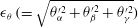${\it\epsilon}_{{\it\theta}}\,(=\sqrt{{\it\theta}_{{\it\alpha}}^{\prime 2}+{\it\theta}_{{\it\beta}}^{\prime 2}+{\it\theta}_{{\it\gamma}}^{\prime 2}})$ and on averaging we get the fully normalized form of the scalar-gradient evolution equation, which is appropriate for our study:

(3.18) $$\begin{eqnarray}\displaystyle \left<\frac{1}{{\it\epsilon}_{{\it\theta}}^{2}}\frac{\text{d}}{\text{d}t^{\prime }}\left(\frac{\partial {\it\theta}^{\prime }}{\partial x_{j}}\frac{\partial {\it\theta}^{\prime }}{\partial x_{j}}\right)\right> & = & \displaystyle \underbrace{\left<-\frac{2\left({\it\alpha}{\it\theta}_{{\it\alpha}}^{\prime 2}+{\it\beta}{\it\theta}_{{\it\beta}}^{\prime 2}+{\it\gamma}{\it\theta}_{{\it\gamma}}^{\prime 2}\right)}{{\it\epsilon}_{{\it\theta}}^{2}}\right>}_{\text{I}}-\underbrace{\left<\frac{2}{3}{\it\Pi}\right>}_{\text{II}}\nonumber\\ \displaystyle & & \displaystyle +\,\underbrace{\left<\frac{1}{{\it\epsilon}_{{\it\theta}}^{2}}\frac{2D}{{\it\epsilon}}\frac{\partial }{\partial x_{i}}\left(\frac{1}{{\it\rho}}\frac{\partial ^{2}{\it\theta}^{\prime }}{\partial x_{k}\partial x_{k}}\right)\frac{\partial {\it\theta}^{\prime }}{\partial x_{i}}\right>}_{\text{III}}.\end{eqnarray}$$

The influence of various mechanisms on the evolution of the scalar gradient is now evident.

1. (1) The velocity-gradient magnitude directly affects the time scale of mixing in term III. Since term III collectively represents effects arising because of the random molecular motion on the scalar-gradient magnitude, we refer to this term as the viscous mechanism.

2. (2) The term marked II represents the influence of dilatation on the scalar-gradient evolution. In contracting fluid elements ( $\unicode[STIX]{x1D622}_{ii}<0$ ), this mechanism enhances scalar dissipation, and has the opposite effect in expanding regions. This mechanism is inconsequential in volume-preserving fluid elements. Since this term represents the effect of only the isotropic portion of the velocity-gradient tensor, we call this term the isotropic amplification mechanism.

3. (3) The streamline topology manifested via the anisotropic strain-rate eigenvalues and principal directions influences the production of scalar dissipation via the term marked I. Since ${\it\alpha}+{\it\beta}+{\it\gamma}=0$ , one eigenvalue ( ${\it\alpha}$ ) is guaranteed to be positive and another ( ${\it\gamma}$ ) is certain to be negative. Interactions that cause strong alignment between the scalar gradient and the ${\it\gamma}$ eigenvector lead to positive production and enhanced mixing. Strong alignment between the scalar gradient and the ${\it\alpha}$ vector will diminish the mixing. Since this term represents the effect of only the anisotropic portion of the velocity-gradient tensor, we call this term the anisotropic nonlinear amplification mechanism.

It is evident that the mixing efficiency and scalar dissipation following a fluid particle are strongly contingent upon the velocity-gradient history of that particle. Therefore, it is appropriate to condition the process on the velocity-gradient history of the fluid particle. Statistical conditioning based upon the fluid-particle velocity history represents a daunting task. The local (particle) streamline topology serves as a viable surrogate for the fluid-particle velocity-gradient history. Therefore, towards understanding and modelling scalar mixing, it is expedient to examine the amplification mechanisms of scalar dissipation conditioned upon local topology. Towards this end, we next characterize the mixing characteristics conditioned upon different topologies and normalized dilatational levels by employing direct numerical simulations of scalar mixing in homogeneous compressible turbulence.

4 Direct numerical simulations and plan of study

We employ the direct numerical simulations (DNS) of decaying isotropic turbulence of Kumar, Girimaji & Kerimo (Reference Kumar, Girimaji and Kerimo2013) for examining mixing statistics conditioned upon the local flow topology and dilatation. These simulations have been performed using a solver based on the gas kinetic method (GKM). The GKM was proposed originally by Xu (Reference Xu1998) for unsteady compressible flows. The GKM is based on the Boltzmann evolution equation of the velocity distribution function, and uses the Bhatnagar–Gross–Krook (BGK) collision operator in conjunction with the state equation of a calorically perfect gas. Further details on the GKM method itself as well as the solver are available in Kumar et al. (Reference Kumar, Girimaji and Kerimo2013).

Table 2.

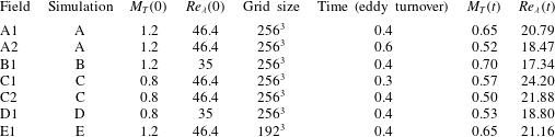
Description of the simulation cases and the extracted flow fields. Here, $M_{T}(0)$ and $Re_{{\it\lambda}}(0)$ represent the initial values of these quantities, whereas $M_{T}(t)$ and $Re_{{\it\lambda}}(t)$ represent the values at the instant flow fields are extracted from the respective simulations for investigation. The reported field extraction time is a fraction of the eddy turnover time of the respective simulation.

Our computational domain is a cubic box with periodic boundary conditions on opposite sides of the domain. The initial velocity field is chosen to have zero mean and a spectrum $(E({\it\kappa}))$ of the following form:

(4.1) $$\begin{eqnarray}E({\it\kappa},t=0)=S{\it\kappa}^{4}\exp (-T{\it\kappa}^{2}),\quad {\it\kappa}=\sqrt{{\it\kappa}_{x}^{2}+{\it\kappa}_{y}^{2}+{\it\kappa}_{z}^{2}},\end{eqnarray}$$

wherein initially only a narrow band of wavenumbers $({\it\kappa})$ is energized: ${\it\kappa}\in [1,8]$ . Here, $S$ and $T$ represent spectrum constants. The scalar field too is initialized as a random field with zero mean.

Decaying compressible turbulence is parametrized by the turbulent Mach number ( $M_{T}$ ) and the Reynolds number based on the Taylor microscale $(Re_{{\it\lambda}})$ . These quantities are defined as

(4.2a,b ) $$\begin{eqnarray}M_{T}=\sqrt{\frac{2k}{nR\left<T\right>}},\quad Re_{{\it\lambda}}=\sqrt{\frac{20}{3{\it\varepsilon}{\it\nu}}}k,\end{eqnarray}$$

where $k$ and ${\it\varepsilon}$ represent the turbulent kinetic energy and its dissipation rate respectively and ${\it\nu}$ represents the kinematic viscosity. Seven flow fields extracted from five different simulations are employed for this study. A description of these flow fields and simulations is presented in table 2. The initial $M_{T}$ and $Re_{{\it\lambda}}$ values of the five simulations are in the ranges 0.8–1.2 and 35–46.4 respectively. In decaying compressible turbulence, since the instantaneous Mach and Reynolds numbers continuously evolve with time, these values can be significantly different from their initial values. In table 2, we have also included the instantaneous values of the Mach number and the Reynolds number of the extracted flow fields.

Figure 2.

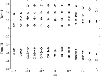
Mean values of terms I and III of (3.18) conditioned on the topology ( ${\it\Gamma}$ ) and the normalized dilatation ( $\unicode[STIX]{x1D622}_{kk}$ ): ○, UNSS; ▫, SNSS; ▵, SFS; $\times$ , UFC; $\ast$ , UFS; ♢, SFC. Large symbols: second order from field A1. Small symbols: fourth order from field A1.

Table 3.

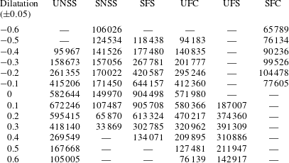
Sample sizes (field A1). A dash indicates a non-existent topology or an unviably small sample size.

After extracting the velocity and scalar fields at a chosen time instant, the required velocity and scalar gradients are computed. The results are then conditionally sampled based on the values of the normalized dilatation rate ( $\unicode[STIX]{x1D622}_{ii}$ ) and topology ( ${\it\Gamma}$ ). Subsequently, these samples are used to compute conditional averages and probability density functions (p.d.f.s) of various quantities of interest appearing in (3.18). In table 3, we present sample sizes from field A1 for all possible topologies at discrete normalized dilatation levels.

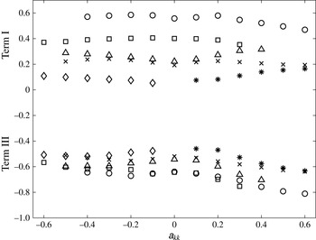
Care is taken to ensure that each simulation is well resolved and the computed statistics are within acceptable levels of accuracy. Our study requires investigation of the statistics of the velocity gradients (topology and dilatation), the product of the scalar and velocity gradients (term I in (3.18)), and higher-order gradients of the scalar gradient (term III in (3.18)). In figure 2, we demonstrate that the mean values of terms I and III conditioned upon the topology and normalized dilatation show negligible difference when the derivatives are computed using second-order or fourth-order discretization formulae (field A1). The results presented in the rest of this paper thus employ fourth-order discretization formulae. In figure 3, we present mean values of terms I and III conditioned upon the topology and normalized dilatation obtained from fields A1 and E1. The corresponding two simulations (A and E) are identical in terms of initial conditions and differ only in terms of grid size. Simulation A employs a grid size of $256^{3}$ , whereas simulation E employs a grid size of $192^{3}$ . Both flow fields have been extracted at the same time instant of 0.4 eddy turnover times in each simulation. Evidently, the mean values of both of the terms (I and III) from simulation E lie close to the corresponding values from simulation A for each topology at almost all dilatation levels. We deem this level of accuracy adequate for this study and for the ensuing conclusions.

Figure 3.

Mean values of terms I and III of (3.18) conditioned on the topology ( ${\it\Gamma}$ ) and the normalized dilatation ( $\unicode[STIX]{x1D622}_{kk}$ ): ○, UNSS; ▫, SNSS; ▵, SFS; $\times$ , UFC; $\ast$ , UFS; ♢, SFC. Small symbols: field A1. Large symbols: field E1.

5 Behaviour of the amplification and viscous mechanisms

In this section, we study the influence of the topology, normalized dilatation, Mach number and Reynolds number on the locally normalized evolution equation of scalar dissipation (3.18). Of the three mechanisms appearing on the right-hand side of (3.18), the physics of the isotropic amplification mechanism (term II) is straightforward. In its normalized form, this mechanism is an explicit function of $\unicode[STIX]{x1D622}_{ii}$ alone. Clearly, irrespective of Mach number, Reynolds number or topology its value conditioned upon the normalized dilatation is governed exclusively by the normalized dilatation itself. For expanding particles, this mechanism causes a decrease in the scalar dissipation, and in contracting particles, it causes a growth of the scalar dissipation. For volume-preserving fluid elements, this mechanism does not have any influence on the scalar dissipation. The other two mechanisms (terms I and III), however, are mathematically more complex and, thus, require a more detailed study, which we present in the next subsections.

5.1 Anisotropic nonlinear amplification mechanism

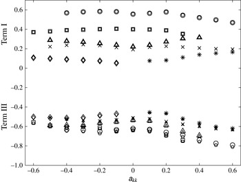
The anisotropic amplification mechanism (term I in (3.18)) involves tensorial interactions between the scalar-gradient vector and the anisotropic strain-rate tensor. This interaction is dependent on the eigenvalues of $\unicode[STIX]{x1D634}_{ij}^{a}$ and the direction cosines of the scalar-gradient vector (3.18) resolved in the principal coordinate system of $\unicode[STIX]{x1D634}_{ij}^{a}$ . In figure 4, we present averaged values of term I jointly conditioned upon the normalized dilatation and topology as seen in simulation A at 0.4 eddy turnover times (field A1). The figure clearly shows that, irrespective of the normalized dilatation or topology, the contribution of this mechanism is always positive, and thus enhances the scalar dissipation for all expanding, contracting as well as volume-preserving fluid elements. Upon further closer examination, we observe that the conditional mean of term I shows a strong dependence on the topology but a relatively much weaker dependence on the normalized dilatation. In figure 4, we observe that the anisotropic mechanism of non-focal topologies (UNSS and SNSS) is higher than that of focal topologies. Clearly, among all topologies, UNSS shows the highest conditional mean values at all dilatation levels. The contributions from SFS and UFC are almost equal. The weakest contributor at negative dilatation levels is SFC, whereas at positive dilatation levels UFS is the weakest contributor.

Figure 4.

Mean values of term I (all values are positive) and term III (all values are negative) of (3.18) conditioned on the topology ( ${\it\Gamma}$ ) and normalized dilatation ( $\unicode[STIX]{x1D622}_{kk}$ ): ○, UNSS; ▫, SNSS; ▵, SFS; $\times$ , UFC; $\ast$ , UFS; ♢, SFC (field A1).

Figure 5.

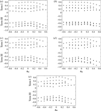
Mean values of term I (all values are positive) and term III (all values are negative) of (3.18) conditioned on the topology ( ${\it\Gamma}$ ) and normalized dilatation ( $\unicode[STIX]{x1D622}_{kk}$ ): ○, UNSS; ▫, SNSS; ▵, SFS; $\times$ , UFC; $\ast$ , UFS; ♢, SFC. (a) Field A2, (b) field B1, (c) field C1, (d) field C2 and (e) field D1.

To examine the influence of the Mach number and Reynolds number on the conditional statistics of term I, in figure 5(a–e) we plot statistics extracted from other flow fields considered in this work (fields A2, B1, C1, C2 and D1). Evidently, all of the figures show almost identical behaviour of the conditional mean of term I. Thus, based on these observations we conclude that the locally normalized anisotropic amplification mechanism (term I) demonstrates almost universal behaviour independent of Mach number and Reynolds number. The authors believe that this universal behaviour of the anisotropic nonlinear mechanism can possibly be leveraged to arrive at closure models for this term. Indeed, such an attempt is made in § 6 of this work.

5.1.1 Alignment of the scalar gradient with the strain-rate eigenvectors

Figure 6.

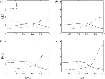
The p.d.f.s of the cosine of the angle between the scalar-gradient vector and the eigenvectors of the anisotropic strain-rate tensor conditioned upon $|\unicode[STIX]{x1D622}_{ii}|<0.05$ and (a) UFC, (b) SFS, (c) SNSS and (d) UNSS (field A1).

Figure 7.

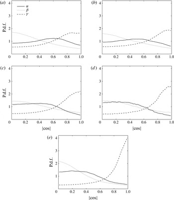
The p.d.f.s of the cosine of the angle between the scalar-gradient vector and the eigenvectors of the anisotropic strain-rate tensor conditioned upon $\unicode[STIX]{x1D622}_{ii}\geqslant 0.05$ and (a) UFS, (b) UFC, (c) SFS, (d) SNSS and (e) UNSS (field A1).

Figure 8.

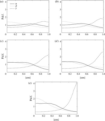
The p.d.f.s of the cosine of the angle between the scalar-gradient vector and the eigenvectors of the anisotropic strain-rate tensor conditioned upon $\unicode[STIX]{x1D622}_{ii}\leqslant -0.05$ and (a) SFC, (b) UFC, (c) SFS, (d) SNSS and (e) UNSS (field A1).

Ashurst et al. (Reference Ashurst, Kerstein, Kerr and Gibson1987) have earlier investigated the statistics of scalar-gradient alignment in the context of incompressible turbulence. With the motivation of further understanding the trends shown by the anisotropic amplification mechanism seen in figure 4, we examine the alignment tendencies between the scalar-gradient vector and the anisotropic strain-rate eigenvectors in compressible decaying turbulence. Since ${\it\alpha}+{\it\beta}+{\it\gamma}=0$ , ${\it\gamma}$ is guaranteed to be negative and ${\it\alpha}$ is certain to be positive. Thus, from the point of view of maximizing the growth rate of scalar dissipation, it would be desirable to have the scalar-gradient vector (i) well aligned with the ${\it\gamma}$ eigenvector and/or (ii) poorly aligned with the ${\it\alpha}$ eigenvector. At this point it is worth examining whether the higher values of the anisotropic mechanism in the non-focal topologies (UNSS and SNSS) are indeed attributable to the changing conditional alignment tendencies of the scalar-gradient vector in compressible turbulence.

In figures 6–8, we present the probability density functions of the cosines of the angles between the scalar-gradient vector and the ${\it\alpha}$ , ${\it\beta}$ and ${\it\gamma}$ eigenvectors of the local anisotropic strain-rate tensor jointly conditioned upon the sign of dilatation and various topologies. Figure 6(a–d) presents the p.d.f.s conditioned on $\unicode[STIX]{x1D622}_{ii}=0$ and the four possible topologies. All of these figures have been obtained by employing the flow field extracted from simulation A at 0.4 eddy turnover times (field A1). We observe that the alignment tendency of the scalar-gradient vector monotonically increases in the following order: UFC  ${<}$  SFS  ${<}$  SNSS  ${<}$  UNSS. This is indeed the same order in which the anisotropic amplification mechanism increases in figure 4. Exactly the same behaviour is seen in expanding and contracting fluid elements as well (figures 7 and 8). In all cases, the non-focal strain-dominated topologies enhance this alignment much more than the focal topologies. Thus, based on these results we conclude that the variation in the anisotropic production mechanism of scalar dissipation is indeed attributable to the ability of a topology to enhance the alignment between the scalar-gradient tensor and the ${\it\gamma}$ eigenvector of the anisotropic strain-rate tensor.

Although we have presented the conditional p.d.f.s in figures 6–8 using the flow field from simulation A at 0.4 eddy turnover times (field A1) only, these statistics have been carefully examined in all other fields as well, B1, C1, C2, D1 and A2. We find that the conditional p.d.f.s of the angles between the scalar-gradient vector and the strain-rate eigenvectors are almost identical in all six flow fields considered in this study. Thus, we conclude that, like the conditional averages of term I (figure 4), the conditional p.d.f.s of the angles between the scalar-gradient vector and the strain-rate eigenvectors are also fairly independent of Mach number and Reynolds number (at least over the range of these parameters considered in this work).

6 Conditional scalar statistics: kinematic analysis and modelling

In its normalized form, the isotropic amplification mechanism (term II in (3.18)) depends solely on the trace of the velocity-gradient tensor, and there is no explicit or implicit dependence on the scalar concentration or its gradients (3.18). However, the anisotropic mechanism does have an explicit dependence on a passive scalar or its gradients. This dependence comes through the direction cosines of the scalar-gradient vector with respect to the principal coordinate system of the strain-rate tensor. From a modelling point of view, it is pertinent to explore whether it is possible to approximate the behaviour of the anisotropic mechanism solely in terms of the velocity-gradient tensor itself. The results of § 5 provide us with convincing evidence about the dominant role played by the ${\it\gamma}$ eigenvector in shaping the behaviour of the anisotropic mechanism – the magnitude of the anisotropic production mechanism is strongly correlated with the extent of alignment between the scalar-gradient vector and the ${\it\gamma}$ eigenvector. Based on these observations, we now attempt to simplify the expression of the anisotropic mechanism in such a way that it can be modelled in terms of the velocity-gradient tensor alone. Although similar modelling attempts have been made earlier in the context of incompressible turbulence (Fox Reference Fox1997, Reference Fox1999; Vedula et al. Reference Vedula, Yeung and Fox2001; Yeung Reference Yeung2002), to the best of the authors’ knowledge no such model exists for compressible turbulence.

If $l$ , $m$ , and $n$ are the direction cosines of the scalar-gradient vector in the principal coordinate system of the strain-rate tensor, then the anisotropic term of (3.18) can be expressed as

(6.1) $$\begin{eqnarray}-2\frac{{\it\alpha}{\it\theta}_{{\it\alpha}}^{\prime 2}+{\it\beta}{\it\theta}_{{\it\beta}}^{\prime 2}+{\it\gamma}{\it\theta}_{{\it\gamma}}^{\prime 2}}{{\it\epsilon}_{{\it\theta}}^{2}}=-2\left({\it\alpha}l^{2}+{\it\beta}m^{2}+{\it\gamma}n^{2}\right),\end{eqnarray}$$

where

(6.2) $$\begin{eqnarray}l^{2}+m^{2}+n^{2}=1.\end{eqnarray}$$

In the alignment visualizations of figures 6–8, we have seen that for almost all topologies the scalar-gradient vector is approximately orthogonal to the ${\it\beta}$ eigenvector, thus

(6.3.a,b ) $$\begin{eqnarray}m^{2}\approx 0\quad \text{and}\quad l^{2}\approx 1-n^{2}.\end{eqnarray}$$

Further, ${\it\alpha}$ , ${\it\beta}$ and ${\it\gamma}$ $({\it\alpha}>{\it\beta}>{\it\gamma})$ are eigenvalues of the anisotropic strain-rate tensor, which implies

(6.4) $$\begin{eqnarray}{\it\alpha}+{\it\beta}+{\it\gamma}=0.\end{eqnarray}$$

Thus, using (6.3) and (6.4), we write (6.1) as

(6.5) $$\begin{eqnarray}-2\frac{{\it\alpha}{\it\theta}_{{\it\alpha}}^{\prime 2}+{\it\beta}{\it\theta}_{{\it\beta}}^{\prime 2}+{\it\gamma}{\it\theta}_{{\it\gamma}}^{\prime 2}}{{\it\epsilon}_{{\it\theta}}^{2}}\approx -2\left\{{\it\gamma}\left(2n^{2}-1\right)+{\it\beta}\left(n^{2}-1\right)\right\}.\end{eqnarray}$$

Since the anisotropic mechanism depends strongly on the topology and mildly on the normalized dilatation (figure 4), we make a modelling assumption that the anisotropic amplification mechanism is an explicit function of the topology $({\it\Gamma})$ alone:

(6.6) $$\begin{eqnarray}-2\left<\left.\frac{{\it\alpha}{\it\theta}_{{\it\alpha}}^{\prime 2}+{\it\beta}{\it\theta}_{{\it\beta}}^{\prime 2}+{\it\gamma}{\it\theta}_{{\it\gamma}}^{\prime 2}}{{\it\epsilon}_{{\it\theta}}^{2}}\right|_{{\it\Gamma},\unicode[STIX]{x1D622}_{ii}}\right>\approx -2\left<\left.\frac{{\it\alpha}{\it\theta}_{{\it\alpha}}^{\prime 2}+{\it\beta}{\it\theta}_{{\it\beta}}^{\prime 2}+{\it\gamma}{\it\theta}_{{\it\gamma}}^{\prime 2}}{{\it\epsilon}_{{\it\theta}}^{2}}\right|_{{\it\Gamma}}\right>.\end{eqnarray}$$

With (6.5) and (6.6),

(6.7) $$\begin{eqnarray}-2\left<\left.\frac{{\it\alpha}{\it\theta}_{{\it\alpha}}^{\prime 2}+{\it\beta}{\it\theta}_{{\it\beta}}^{\prime 2}+{\it\gamma}{\it\theta}_{{\it\gamma}}^{\prime 2}}{{\it\epsilon}_{{\it\theta}}^{2}}\right|_{{\it\Gamma},\unicode[STIX]{x1D622}_{ii}}\right>\approx -2\left<{\it\gamma}\left(2n^{2}-1\right)|_{{\it\Gamma}}\right>-2\left<{\it\beta}\left(n^{2}-1\right)|_{{\it\Gamma}}\right>.\end{eqnarray}$$

Table 4.

Comparison of product of averages and average of product conditioned upon topology (field A1).

Now, to further simplify the right-hand side of (6.7), we compare the values of $\langle {\it\gamma}|_{{\it\Gamma}}\rangle \langle n^{2}|_{{\it\Gamma}}\rangle$ with $\langle {\it\gamma}n^{2}|_{{\it\Gamma}}\rangle$ , and $\langle {\it\beta}|_{{\it\Gamma}}\rangle \langle n^{2}|_{{\it\Gamma}}\rangle$ with $\langle {\it\beta}n^{2}|_{{\it\Gamma}}\rangle$ in table 4. We observe that

(6.8a,b ) $$\begin{eqnarray}\langle {\it\gamma}n^{2}|_{{\it\Gamma}}\rangle \approx \langle {\it\gamma}|_{{\it\Gamma}}\rangle \langle n^{2}|_{{\it\Gamma}}\rangle \text{and }\langle {\it\beta}n^{2}|_{{\it\Gamma}}\rangle \approx \langle {\it\beta}|_{{\it\Gamma}}\rangle \langle n^{2}|_{{\it\Gamma}}\rangle .\end{eqnarray}$$

This observation when combined with (6.6) and (6.7) leads us to the following model:

(6.9) $$\begin{eqnarray}-2\left\langle \left.\frac{{\it\alpha}{\it\theta}_{{\it\alpha}}^{\prime 2}+{\it\beta}{\it\theta}_{{\it\beta}}^{\prime 2}+{\it\gamma}{\it\theta}_{{\it\gamma}}^{\prime 2}}{{\it\epsilon}_{{\it\theta}}^{2}}\right|_{{\it\Gamma},\unicode[STIX]{x1D622}_{ii}}\right>\approx \left<{\it\gamma}|_{{\it\Gamma}}\right\rangle C({\it\Gamma})+\left<{\it\beta}|_{{\it\Gamma}}\right>D({\it\Gamma}),\end{eqnarray}$$

where $C$ and $D$ are model coefficients dependent on the topology $({\it\Gamma})$ . It should be noted that there is no explicit appearance of scalar-gradient direction cosines in the model expression of (6.9). Thus, in line with our objective, the modelling conjecture attempts to recover the behaviour of the anisotropic nonlinear amplification mechanism based solely on the velocity-gradient parameters ${\it\gamma}$ and ${\it\beta}$ , and the model constants $C$ and $D$ , which in turn depend on the topology only.

Table 5.

The constants $C$ and $D$ for different topologies computed using the least-squares method and data from field A1.

Figure 9.

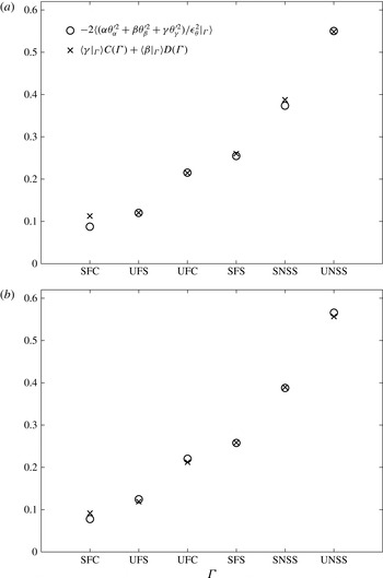
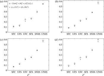
Comparison of the left-hand side and right-hand side of the model equation (6.9) from (a) field A1 and (b) field A2.

For a given topology, data points corresponding to the anisotropic mechanism at various normalized dilatations of figure 4 can now be used as sample points to perform a least-squares analysis with the left-hand side of (6.9) as dependent and $\langle {\it\gamma}|_{{\it\Gamma}}\rangle$ and $\langle {\it\beta}|_{{\it\Gamma}}\rangle$ as independent variables. Such an analysis can be used to estimate $C({\it\Gamma})$ and $D({\it\Gamma})$ for each individual topology. In table 5, we tabulate the values of $C({\it\Gamma})$ and $D({\it\Gamma})$ obtained by using field A1. Thus, (6.9) with the values of $C$ and $D$ presented in table 5 is the proposed model for the anisotropic nonlinear amplification mechanism (term I in (3.18)).

In figure 9(a), we plot the conditional means of the anisotropic mechanism at 0.4 eddy turnover times of simulation A (field A1) along with the model calculations. The agreement is good. This is expected because the model constants $C({\it\Gamma})$ and $D({\it\Gamma})$ have been obtained using the flow-field data at the same time instant. Thus, a reasonable test of the model can be performed by comparing the model calculations using the same values of the constants $C$ and $D$ (as given in table 5) but using the velocity-gradient field extracted at another time instant of simulation A. In figure 9(b), we present the conditioned anisotropic mechanism using DNS data at 0.6 eddy turnover times from simulation A (field A2). The figure also shows the model calculations. Clearly, the agreement is good at 0.6 eddy turnover times as well, suggesting the viability of the proposed modelling approach. Further evaluations of the model are performed in figure 10. Here, we employ the same model constants (table 5), but we use the flow fields B1, C1, C2 and D1. The model predictions agree reasonably well with the flow-field statistics in each of these four flow fields. This clearly demonstrates the robustness and validity of the proposed modelling approach.

Figure 10.

Comparison of the left-hand side and right-hand side of the model equation (6.9). (a) Field B1, (b) field C1, (c) field C2 and (d) field D1.