1. Introduction

Signaling games model simple signaling interactions between a sender and a receiver. They emphasize the social aspects of language. Thus, they are able to provide basic insights into some fundamental questions concerning the explanation of how meaningful communication can emerge. The importance of societal relations for the emergence of communication was already pointed out by David Hume (Reference Hume1739), Jean-Jacques Rousseau (Reference Rousseau1755), and Adam Smith (Reference Smith1761). It was further elaborated in David Lewis's (Reference Lewis1969) seminal work on conventions. One main idea underlying this view is that a basic function of language is to facilitate coordinated behavior. Meaning is thus a consequence of pragmatic factors.

Lewis (Reference Lewis1969) was intended as an answer to Quine's (Reference Quine and Lee1936) counterarguments against the logical positivist's claim that conventions of meaning form the basis of logical truth and logical inference. One way to express Quine's skepticism is to doubt that the truth of a statement is given by a linguistic component and a factual component (Quine Reference Quine1953). Analytical statements have zero factual component. They are true regardless of how the world looks. The linguistic component of the truth of a statement is governed by conventions of meaning. But do we have a good explanation of how conventions of meaning come about?

According to Quine and others, we do not have such an explanation (see White Reference White and Hook1950; a similar argument can already be found in Rousseau [Reference Rousseau1755]). There is no noncircular explanation of conventions of meaning. Conventions come about by agreement. To achieve agreement we always have to presuppose some kind of rudimentary language, which is itself left unexplained. One of Lewis's basic insights—which can, in fact, be traced back to Hume—is that conventions need not come about by agreement. They might be stable outcomes of repeated nonverbal interactions. Or they might be salient among their alternatives.

This paper continues Skyrms's (Reference Skyrms1996, Reference Skyrms2000, Reference Skyrms2004) analysis of the explanation of meaning conventions in evolutionary terms. I shall argue that an evolutionary explanation avoids the difficulties that an explanation in terms of rational choice (like Lewis's account) faces at a very fundamental level. As such, the position underlying this study is the one mentioned above, to wit, that meaning is a consequence of pragmatic factors. By this I mean that meaning emerges from the interactions of less than fully rational agents (i.e., agents who are constrained in their computing capacities and in the information they have about the structure of the game). These agents may be less deliberate than their fully rational kin in standard game theory. However, they might still be said to maximize their utility within constraints that are not assumed in standard game theory. In this sense, my analysis might be called pragmatic.

The arguments in this direction will be substantiated by reporting a number of theorems on simple signaling games and signaling games that allow probabilistic associations between states, signals, and acts. Both kinds of signaling games allow for states with no communication, states with partial communication, and states with perfect communication. My main results show that, except for one special case, the latter two types of states emerge with positive probability under selection dynamics. States with no communication are always dynamically unstable. States of partial communication can be destabilized by neutral drift. States of perfect communication turn out to be the only states that are robust relative to selection and drift.

I will start in Section 2 by defining simple signaling games and reviewing some of their properties. In Sections 3 and 4 I shall discuss language conventions with respect to evolution and rational choice. This discussion will be a methodological background to the study of the dynamics of simple and generalized simple signaling games in Sections 5 and 6, where the main new results can be found. Section 7 concludes by reconsidering the explanatory value of my results.

2. Simple Signaling Games

Simple signaling games are based on coordination problems between states and acts. The simplest situation of this kind consists of two states of the world, $\sigma _{1}$ and $\sigma _{2}$ , and two corresponding acts, $\alpha _{1}$ and $\alpha _{2}$ . Each act is a proper response to exactly one of the states. An individual who chooses the wrong act gets no positive payoff. This payoff structure is illustrated in Table 1. Let us call a situation like this one a “state-act coordination problem.”

Table 1.A State-Act Coordination Problem with a > 0.

	α1	α2
σ1	a	0
σ2	0	a

Suppose that there are two individuals. The sender observes the state while the receiver chooses an act. The latter cannot observe the state. The sender can send two messages, $m_{1}$ and $m_{2}$ , to indicate which state has occurred. The receiver might respond to each of the signals by choosing a particular act. If the receiver chooses the right act, then both players get the same payoff a ( $a> 0$ ). Since the sender and the receiver always get the same payoff, it is in the sender's interest to communicate which state has occurred. Likewise, the receiver has an interest to associate the signal with the right act. So they need a common understanding about the two signals in order to coordinate their actions.

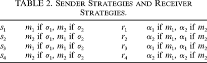
The situation outlined above constitutes a simple signaling game with two players, the sender and the receiver, two states of the world, two messages, and two acts. A sender strategy specifies, for each state, what signal to send. A receiver strategy specifies which act will be chosen as a response to a message. Accordingly, there are four sender strategies and four receiver strategies. The sender might send one of the two signals if $\sigma _{1}$ occurs and the other one if $\sigma _{2}$ occurs, or she might always send the same signal regardless of which state occurs. The receiver might choose one of the two acts as a response to $m_{1}$ and the other act as a response to $m_{2}$ , or she might ignore the message and always choose the same act (see Table 2).

Table 2.Sender Strategies and Receiver Strategies.

$s_{1}$	$m_{1}$ if $\sigma _{1}$ , $m_{2}$ if $\sigma _{2}$	$r_{1}$	α1 if $m_{1}$ , α2 if $m_{2}$
$s_{2}$	$m_{2}$ if $\sigma _{1}$ , $m_{1}$ if $\sigma _{2}$	$r_{2}$	α2 if $m_{1}$ , α1 if $m_{2}$
$s_{3}$	$m_{1}$ if $\sigma _{1}$ , $m_{1}$ if $\sigma _{2}$	$r_{3}$	α1 if $m_{1}$ , α1 if $m_{2}$
$s_{4}$	$m_{2}$ if $\sigma _{1}$ , $m_{2}$ if $\sigma _{2}$	$r_{4}$	α2 if $m_{1}$ , α2 if $m_{2}$

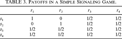
The state-act coordination problem underlying our simple signaling game induces the players’ payoffs. For $a=1$ , these payoffs are illustrated in Table 3. (I shall assume that $a=1$ throughout the paper since this just amounts to a choice of scale.) Notice that we have assumed that each state occurs with probability $1/ 2$ . Each entry represents the signaler's as well as the receiver's payoff. Thus our simple signaling game is a pure coordination game (Lewis Reference Lewis1969).

Table 3.Payoffs in a Simple Signaling Game.

	$r_{1}$	$r_{2}$	$r_{3}$	$r_{4}$
$s_{1}$	1	0	1/2	1/2
$s_{2}$	0	1	1/2	1/2
$s_{3}$	1/2	1/2	1/2	1/2
$s_{4}$	1/2	1/2	1/2	1/2

Simple signaling games based on state-act coordination problems can easily be generalized to signaling problems involving more then two states, acts, and messages. Let $\Pi _{n}=\langle S,\,A,\,u^{*}\rangle $ be an n-state-act coordination problem if $S=\{ \sigma _{1},\,\ldots ,\,\sigma _{n}\} $ is a set of n distinct states of the world, $A=\{ \alpha _{1},\,\ldots ,\,\alpha _{n}\} $ is a set of n distinct acts, and $u^{*}$ is a function that determines the utility of each state-act pair such that $u^{*}(\sigma _{i},\,\alpha _{j}) =\delta _{ij}$ (where the Kronecker symbol $\delta _{ij}=1$ if $i=j$ and $\delta _{ij}=0$ otherwise). In addition, let $M=\{ m_{1},\,\ldots ,\,m_{n}\} $ be a set of n distinct messages and $\mathstrut{\Bbb P} $ be a probability distribution over S such that the probability of each state is positive, $\mathstrut{\Bbb P} (\sigma _{i}) > 0$ for $i=1,\,\ldots ,\,n$ .

The third condition states that the payoffs to each player are generated by the underlying payoff function of the state-act coordination problem by averaging each player's payoff in each of the states $\sigma _{i}$ according to $\sigma _{i}$ 's probability of occurrence (the second argument of $u^{*}$ determines the act chosen by the receiver as a response to the signaler's message). Thus, the payoff from a particular strategy combination is the expected value of the payoffs associated with the state-act pairs that result from this strategy combination relative to the probability distribution $\mathstrut{\Bbb P} $ .

Signaling systems are combinations of sender strategies and receiver strategies that deserve special attention (Lewis Reference Lewis1969). They guarantee that both players get the maximum payoff regardless of which state of the world occurs. If the players employ a signaling system, they are fully coordinated by virtue of the signals. In the example above (see Table 3), there are two signaling systems, $(s_{1},\,r_{1}) $ and $(s_{2},\,r_{2}) $ .

Equivalently, we may call $(s_{k},\,r_{l}) $ a signaling system if and only if $u^{*}(\sigma _{j},\,(r_{l}\circ s_{k}) (\sigma _{j})) =1$ for all $j=1,\,\ldots ,\,n$ .

Call $s_{i}$ (or $r_{j}$ ) a part of a signaling system if and only if there is an $r_{k}$ (or $s_{l}$ ) such that $(s_{i},\,r_{k}) $ (or $(s_{l},\,r_{j}) $ ) is a signaling system. Then it is obvious that the following holds:

According to Lewis (Reference Lewis1969), Skyrms (Reference Skyrms1996), Vanderschraaf (Reference Vanderschraaf1998), and Young (Reference Young1998), a behavioral regularity is conventional if everybody has an interest to act in accordance with it and if it has an alternative (i.e., it involves some kind of arbitrariness). This intuition can be quite naturally captured in game-theoretic terms. A Nash equilibrium is a combination of strategies in which no player would gain by unilaterally deviating from her part of the equilibrium. A strict Nash equilibrium is a Nash equilibrium in which each player would do worse by unilaterally choosing a strategy different from her equilibrium strategy. In a pure coordination game with at least two strict Nash equilibria, each of the two strict Nash equilibria is a candidate for a convention. In a simple signaling game, for instance, each player does strictly better in a signaling system equilibrium and no player has an interest that the other player deviates from it since she would also be worse off in this case.Footnote ¹

In the example above (see Table 3) there are two strict Nash equilibria, $(s_{1},\,r_{1}) $ and $(s_{2},\,r_{2}) $ , and four pure nonstrict Nash equilibria, $(s_{3},\,r_{3}) $ , $(s_{3},\,r_{4}) $ , $(s_{4},\,r_{3}) $ , and $(s_{4},\,r_{4}) $ . The two strict Nash equilibria are also the two signaling systems and, hence, the two possible signaling conventions of this game. This result holds with some generality (as has already been pointed out in Skyrms [Reference Skyrms1996, 83]).

Thus, if conventions in signaling games are strict Nash equilibria, the only candidates for conventions in simple signaling games are signaling systems. In a population of individuals who are repeatedly playing a simple signaling game, a signaling system is a simple conventional language. The population could have adopted another signaling system that would have done essentially the same job. But whatever signaling system they have, they understand each other by virtue of a convention.

3. Stability and Emergence of Language Conventions

At this point two questions become pressing: How is a conventional language maintained in a population? And how might a conventional language be established in the first place? These two questions concern conventions in general. It is not enough to state what the candidates for conventions in a particular game are if we want to explain why one of the possible conventions is in fact a convention in a population. To do this, we have to explain how this convention has emerged and why it is stable.

These questions become particularly pressing if the candidates for conventions are entirely symmetric as they are in a simple signaling game. There is no reason to choose one of the possible signaling conventions rather than another since any signaling system does the same job. But if there is no reason to choose one of the language conventions rather than another, how will individuals decide on one of them without communication? And, once the decision is made, why do they not switch? This scenario is one instance of what Skyrms (Reference Skyrms1996) calls the “curse of symmetry.”

Lewis (Reference Lewis1969) proposes an answer to these questions in terms of rational choice theory and in terms of salience. According to Lewis, the stability of conventions is guaranteed because the structure of the game, the payoffs, and the rationality of the players are common knowledge. A fact F is common knowledge among agents A and $A^{\prime }$ if A knows that F, and A knows that $A^{\prime }$ knows that F, and A knows that $A^{\prime }$ knows that A knows that F, and so on. The same holds if we interchange A and $A^{\prime }$ . If sender and receiver have common knowledge of the game structure and each other's rationality, they will stick to a signaling convention because there is no room for doubting that the other player is going to stick to her part of the signaling convention.

Following Schelling (Reference Schelling1960), Lewis's answer to the question of how conventional languages are established in the first place is that one of the strict Nash equilibria is a focal point or is salient. It stands out among all equilibria in some psychologically significant respect. That is to say, it is clear to all players that this one equilibrium should be chosen. Here is Lewis's (Reference Lewis1969, 158–159) example for a salient signaling system: Suppose that you come upon a patch of quicksand and you want to warn others who might come there after you. A salient signal would be to put a scarecrow up to the chest into the quicksand.

As Skyrms (Reference Skyrms1996) points out, both of Lewis's answers face serious problems. Concerning the first answer, Skyrms asks where all the common knowledge comes from. It seems to be unclear to what extent players must already understand each other to have this very demanding kind of knowledge. It is possible that we have to assume preexisting communication or something equivalent to it in order to explain that the players understand each other. This would put us back in the position where we need a language to explain the emergence of another language. Hence, without explaining where common knowledge comes from, Lewis's account of why conventions are stable appears to be incomplete, to say the least.

Concerning Lewis's second answer, Skyrms asks where the salient equilibrium is. Sometimes a salient equilibrium might be available, but sometimes not. The harder case is the latter one. For a fundamental investigation a solution to the less hard cases is not enough. (This criticism is a methodological one, but it does not mean that explanations in terms of salience might not be useful in other contexts.) One of the reasons why we set up simple signaling games as involving symmetric strict Nash equilibria was that no one signaling system should stand out. So, to put Skyrms's second criticism in a slightly different way, if there would be a signaling system that is salient to the players, then this should already be expressed in the structure of the game.

Allow me to add a further criticism of salience as an equilibrium selection device. As in the case of common knowledge, it seems unclear to what extent the players must already know about each other in order to view an equilibrium as salient. In terms of signaling systems this means that I must already see the signals as somewhat meaningful or representational within my community. This is, however, the fact to be explained. For instance, in the scarecrow example, one must understand a scarecrow as a representation of ‘me’ (or ‘potentially me’) and the situation as representing ‘me potentially sinking’.

Cubitt and Sugden (Reference Cubitt and Sugden2003) criticize Skyrms's (Reference Skyrms1996) and Vanderschraaf's (Reference Vanderschraaf1998) reconstruction of Lewis's account of convention. First, they show that Lewis's conception of common knowledge does not coincide with the standard infinitely iterated knowledge conception (as described above). Moreover, they try to reestablish salience as an explanation of how conventions start.

Instead of assuming common knowledge, Cubitt and Sugden argue that Lewis tries to derive common knowledge from the agents’ background information and their inductive standards. As they show more formally, “common knowledge in Lewis’ sense is possible only when individuals have reason to believe that, in particular relevant respects, they have common background information and common inductive standards” (Cubitt and Sugden Reference Cubitt and Sugden2003, 185). Given this explanation of common knowledge, we might again ask where the reasons to believe to have common background information and common inductive standards come from, and to what extent this presupposes a mutual understanding that must itself be explained.Footnote ²

As to the role of salience for the selection of strict Nash equilibria, Cubitt and Sugden do not address the criticisms raised above, namely, that assuming salience excludes the worst case scenario for the emergence of conventions and that the prior extent of mutual understanding for salience to be possible is unclear. Thus, it seems that Lewis's account of the emergence and stability of language conventions is deficient in two important respects. This is the point where evolutionary theory comes in.

4. Evolution and Conventions of Language

Skyrms (Reference Skyrms1996) invites us to approach the problem of the emergence and stability of language conventions from an evolutionary standpoint. If an adaptive process governs a population of individuals that are repeatedly confronted with a situation that is similar enough to a signaling game, will one of the signaling systems eventually become established in this population? Biological evidence suggests that the answer to this question is, at least a cautious, yes. Signal coordination is everywhere, from cells communicating via molecules and the honeybee's dance to predator alarm calls of monkeys and bird song (for comprehensive treatments of animal signals, see Snowdon [Reference Snowdon1990], Hauser [Reference Hauser1997], and Maynard Smith and Harper [Reference Maynard Smith and Harper2003]).

The adoption of the evolutionary viewpoint implies that we do not follow Lewis (Reference Lewis1969, 58) and Vanderschraaf (Reference Vanderschraaf1998) in invoking any common knowledge assumptions to define conventions. Instead, we shall say that a population adopts a certain convention if it is a strict Nash equilibrium in a game with at least two strict Nash equilibria and if every individual in the population chooses her actions according to this strict Nash equilibrium. By adopting the evolutionary viewpoint, we also escape the criticisms raised in the previous section. We assume neither that the individuals in the population reach a convention by explicit agreement, nor that they have a preexisting language or common knowledge of the game. Indeed, they may not have much knowledge at all.

The omnipresence of signaling in nature suggests that biological and cultural evolution are likely to be responsible for these phenomena. To get beyond such informal statements, we have to give the problem a clear formulation. Studying the evolutionary dynamics of signaling games seems to be a promising starting point for a first analysis. Skyrms (Reference Skyrms1996) investigates a simple signaling game with two signals by simulating its evolutionary dynamics. In addition, he provides some analytical results in Skyrms (Reference Skyrms2000) for a simplified model of this game. In this model, a signaling system is a global attractor for a population that consists of three types, the signaling system type and two antisignaling types. On the basis of these results one might conjecture that populations will develop a signaling system under evolutionary dynamics for all simple signaling games regardless of the initial state. The results presented in the following section show that this is in general not true for the replicator equations, which are the standard dynamics in formal models of selection.

5. Replicator Dynamics and Signaling Games

If we want to study one population of individuals who can be senders or receivers, we have to consider the symmetrized, or role-conditioned, version of $\Sigma _{n}$ (see, e.g., Cressman Reference Cressman2003). Denote the role-conditioned version of $\Sigma _{n}$ by $\Sigma ^{r}_{n}$ . Going from $\Sigma _{n}$ to $\Sigma ^{r}_{n}$ amounts to assuming that each individual is sender or receiver with probability $1/ 2$ . This is a reasonable assumption as long as we do not impose more structure on the population. If some individuals are in the role of the sender more often than others, then we must say which individuals tend to be senders and which individuals tend to be receivers. For a first analysis of the dynamics of signaling games, imposing such a structure on the population does not seem to be reasonable.

An individual's strategy consists of a sender part $s_{i}$ and a receiver part $r_{j}$ . If a simple signaling game is given, then the strategies of $\Sigma ^{r}_{n}$ are all pairs of strategies of $\Sigma _{n}$ . (This implies that a player's sender strategy need not be consistent with her receiver strategy. She might not be able to “talk to herself.”) Since $\Sigma _{n}$ has $n^{n}$ sender strategies and $n^{n}$ receiver strategies, $\Sigma ^{r}_{n}$ has $n^{2n}$ strategies. For instance, in the example illustrated in Table 3 there are 16 strategies. For $n=3$ , there are already 729 strategies. The payoff to a strategy $(s_{i},\,r_{j}) $ against $(s_{k},\,r_{l}) $ is given by

This is just the expected payoff to a strategy relative to the uniform distribution over the two roles of the game. This specifies $\Sigma ^{r}_{n}$ completely. There are two players. Both can be sender or receiver. Their strategies and payoffs are determined by $\Sigma _{n}$ . Unlike $\Sigma _{n}$ , $\Sigma ^{r}_{n}$ is a symmetric game. This means that the player positions are not distinguishable.

Suppose that a population consists of types of individuals in which each type corresponds to a strategy of $\Sigma ^{r}_{n}$ . Let $\pi (s,\,s^{\prime }) $ be the expected payoff individuals in state s get when meeting individuals of type $s^{\prime }$ . Then s is said to be evolutionarily stable if and only if $\pi (s,\,s) > \pi (s,\,s^{\prime }) $ for all $s^{\prime }\neq s$ ; or if $\pi (s,\,s) =\pi (s,\,s^{\prime }) $ for some $s^{\prime }\neq s$ , then $\pi (s,\,s^{\prime }) > \pi (s^{\prime },\,s^{\prime }) $ (Maynard Smith and Price Reference Maynard Smith and Price1973; Maynard Smith Reference Maynard Smith1982). These conditions guarantee that a large population will not move away from state s once it has reached it. In other words, if a small proportion of individuals are not of type s in a population consisting almost entirely of s, then selection will carry the population back to a state in which only s is present.

By using a result of Selten (Reference Selten1980), Wärneryd (Reference Wärneryd1993) shows that in signaling games, signaling systems and evolutionarily stable states coincide.

Notice that Proposition 5 is an answer to the first question raised in the previous section: Why are language conventions stable? They are stable in a model like that underlying the concept of evolutionary stability because they are evolutionarily stable. In addition, they are the only evolutionarily stable states.

But why should signaling systems emerge in the first place? To answer this question, let us look at the replicator dynamics. The replicator dynamics were introduced in Taylor and Jonker (Reference Taylor and Jonker1978) to highlight the dynamical considerations underlying the evolutionary stability concept (Weibull [Reference Weibull1995] and Hofbauer and Sigmund [Reference Hofbauer and Sigmund1998] are comprehensive treatments of the replicator dynamics).

Let the state of the population be represented by the relative frequencies of the different types. For $\Sigma ^{r}_{n}$ there are $\phi (n) =n^{2n}$ different types. Thus the state of the population is represented as a vector $\mathbf{x}=(x_{1},\,\ldots ,\,x_{\phi (n) }) \in \Delta ^{\phi (n) }$ , where $\Delta ^{\phi (n) }$ is the simplex of $\mathstrut{\Bbb R} ^{\phi (n) }$ :

The interior of $\Delta ^{\phi (n) }$ is the part of $\Delta ^{\phi (n) }$ where all types have positive frequency. It is given by

The boundary of $\Delta ^{\phi (n) }$ is the set where at least one type has zero frequency, that is, $\mathrm{bd}\,(\Delta ^{\phi (n) }) =\Delta ^{\phi (n) }\setminus \mathrm{int}\,(\Delta ^{\phi (n) }) $ . We assume that the population is effectively infinite. Thus, the actual payoff of a type matches its expected payoff. Let $\pi (x_{i},\,\mathbf{x}) $ be the average payoff of type i when the current population state is $\mathbf{x}$ , and let $\pi (\mathbf{x},\,\mathbf{x}) $ be the average payoff of the whole population. The replicator dynamics is a system of differential equations given by

where $\dot{x}_{i}$ denotes the time derivative in the ith component. Hence the frequency of types with above-average payoff increases and the frequency of types with below-average payoff decreases. Equation (1) guarantees that evolution will occur in our population whenever there are fitness differences between types.

The replicator equations (1) were originally introduced to capture biological phenomena. There are, however, a number of studies that show how to make sense of the replicator equations in a cultural context (Binmore, Gale, and Samuelson Reference Binmore, Gale and Samuelson1995; Björnstedt and Weibull Reference Björnstedt, Weibull, Arrow, Colombatto, Perlman and Schmidt1996; Schlag Reference Schlag1998; Harms Reference Harms2004). For example, Björnstedt and Weibull show that a model in which individuals imitate others who have adopted successful strategies leads to a class of dynamics called “monotonic” by taking appropriate limits. This class of dynamics is characterized by the property that strategies yielding a higher payoff have a higher growth rate. The replicator dynamics (1) is monotonic in this sense and may be obtained by choosing specific functional forms for the functions involved in general monotonic dynamics. The system (1) may describe a learning process governed by imitation. Thus (1) seems to be a good point of departure for analyzing signaling interactions in the context of both biological and cultural evolution.

The rest points of a system of ordinary differential equations are the states at which $d\mathbf{x}/ dt$ vanishes. Rest points are fixed points of the flow corresponding to the differential equations. Basically, there are three different kinds of rest points: asymptotically stable, weakly stable, and unstable rest points. An asymptotically stable rest point is characterized by attracting all nearby states. The set of all points that converge to an asymptotically stable rest point is its basin of attraction. If a rest point is weakly or Liapunov stable, then all nearby states stay nearby. (Note that every asymptotically stable rest point is weakly stable, but not vice versa.) Nearby solutions of an unstable state tend away from it (not necessarily in all directions). For details, in particular, facts concerning the relation between stability and eigenvalues, see Hirsch and Smale (Reference Hirsch and Smale1974). There is another concept we will need. A subset F of state space is called an “attractor” if all states sufficiently close to F converge to F. Thus an asymptotically stable rest point is a singleton attractor.

If y is an asymptotically stable state, then the system will tend back to y after a small perturbation. The same is true of any attractor F. If y is Liapunov stable, small perturbations will result in a nearby state. If y is unstable, then small perturbations will lead away from it. Thus asymptotically stable states are meaningful since we can expect the system to be close to one of them after a sufficiently long time.

The rest of this section is devoted to studying the stability properties of the rest points of signaling games under the replicator dynamics (1). As pointed out at the end of the last section, signaling systems will not almost surely emerge in the general case. I will show this by proving that the set of points $\mathbf{x}\in \mathrm{int}\,(\Delta ^{\phi (n) }) $ that does not converge to a signaling system of $\Sigma ^{r}_{n}$ has positive Lebesgue measure. I will identify the sets of points that attract some significant portion of states as being on the boundary. Except for signaling systems, these sets are not attractors, however. Thus it will be important to be cautious when interpreting the results. After stating the relevant theorems, I will try to clarify what they mean for evolutionary explanations of signaling systems. All proofs may be found in the Appendix.

The proof of the first part of Theorem 6 relies on the fact that all rest points in $\mathrm{int}\,(\Delta ^{\phi (n) }) $ for the evolutionary dynamics of signaling games are (linearly) unstable. Notice that Theorem 6 holds for the replicator dynamics of any symmetrized simple signaling game.

Hence, generically interior rest points will not be observed under the replicator dynamics. This situation is analogous to unstable states in statistical mechanics. For instance, the state in which all molecules in a gas are at rest is an unstable equilibrium since any slight perturbation will lead to a state that ultimately converges to mixing. If a population is at an interior rest point for the replicator dynamics of $\Sigma ^{r}_{n}$ , then slight perturbations will carry it to some boundary state.

For a special kind of signaling game with two signals we can in fact prove more:

Thus, almost all solutions will converge to a signaling system under the assumptions of Theorem 7. The next theorem shows that the assumption $\mathstrut{\Bbb P} (\sigma _{1}) =\mathstrut{\Bbb P} (\sigma _{2}) $ is necessary for obtaining this result. The intuition for this is quite simple. If $\mathstrut{\Bbb P} (\sigma _{1}) =p> 1/ 2$ , then the type $z=(s,\,r) $ in which the sender strategy s maps both states on $m_{1}$ and the receiver strategy r maps both messages on $\alpha _{1}$ gets a payoff of p when meeting itself. There are three other types that get p when meeting each other or when meeting z. These types have r as receiver strategy and an arbitrary sender strategy. The payoff of all other types against z is at most p. Although z is unstable (it can be invaded by one of the signaling systems), a mixture of z and a small amount of the other three types with r as receiver strategy will result in a Liapunov stable state $z^{\prime }$ . The reason for this is that for any type w that is not present at $z^{\prime }$ there is at least one type v that is present at $z^{\prime }$ such that $\pi (w,\,v) < p$ . (Details can be found in the Appendix.)

This result reflects the fact that the value of p characterizes the importance of communication for a population playing $\Sigma _{2}$ . If $p=1/ 2$ , then both states have equal weight. Thus coordination of both state-act pairs is equally important to obtain a sufficiently high payoff. This no longer holds for $p\neq 1/ 2$ . In this case, coordination of the state-act pair where the state has higher probability is more important than coordination of the other state-act pair. As $p\rightarrow 1$ (or, alternatively, as $p\rightarrow 0$ ), communication becomes less important. If p is very close to 1, numerical simulations suggest that the measure of the set of points converging to states that are not signaling systems is nearly as large as the basins of attraction for the signaling systems.

If $n> 2$ , nonconvergence to signaling systems of $\Sigma _{n}$ does not depend on $\mathstrut{\Bbb P} $ as in the case of $\Sigma _{2}$ . Moreover, for $n> 2$ , not only subsets of boundary faces are attracting a significant number of initial states. Now all of the interior of a boundary face may consist of Liapunov stable states.

Let us look at one example of such a boundary face. Consider the two types $z_{1}=(s_{1},\,r) $ and $z_{2}=(s_{2},\,r) $ of $\Sigma ^{r}_{3}$ , where $s_{1}$ and $s_{2}$ map $\sigma _{1}$ and $\sigma _{2}$ on $m_{1}$ , $s_{1}$ maps $\sigma _{3}$ on $m_{2}$ , and $s_{2}$ maps $\sigma _{3}$ on $m_{3}$ . r maps $m_{1}$ on $\alpha _{2}$ and $m_{2}$ as well as $m_{3}$ on $\alpha _{3}$ . Then $\epsilon z_{1}+(1-\epsilon) z_{2}$ with $0< \epsilon < 1$ consists entirely of Liapunov stable rest points, and the average payoff on this one-dimensional simplex is $\mathstrut{\Bbb P} (\sigma _{1}) +\mathstrut{\Bbb P} (\sigma _{2}) =r$ . The points on this one-dimensional simplex are Liapunov stable because for any type $w\neq z_{1},\,z_{2}$ , $\pi (w,\,z_{i}) \leq r$ and, in addition, for all w with $\pi (w,\,w) > r$ , $\pi (w,\,z_{i}) =r$ implies $\pi (w,\,z_{j}) < r$ for $i\neq j$ and $i,\,j=1,\,2$ . Thus no mixture of strategies different from $z_{1}$ and $z_{2}$ can destabilize this part of the boundary as long as $0< \epsilon < 1$ .

We have to be cautious in interpreting the results stated in the previous theorems. At first sight they might appear to subvert the thesis that evolution facilitates the emergence of simple communication systems. States of communication are represented by signaling systems. These states do not almost always emerge, however, since a significant portion of initial conditions in $\Delta ^{\phi (n) }$ converges to states that are not signaling systems. Taking a closer look at those suboptimal states reveals that they are not attractors. To see this, suppose that $O\subset \Delta ^{m}$ , $m< \phi (n) $ , is a set of rest points open in $\Delta ^{m}$ such that the set of interior initial conditions converging to O has positive Lebesgue measure. Then $\mathbf{p}^{*}\in O$ is Liapunov stable. Each trajectory starting close to $\mathbf{p}^{*}$ converges to it, stays close to it, or converges to a nearby rest point in O. A basic proposition in evolutionary game theory states that a point is a Nash equilibrium if it is Liapunov stable (Hofbauer and Sigmund Reference Hofbauer and Sigmund1998). Hence $\mathbf{p}^{*}$ is a Nash equilibrium. Let e and $e^{\prime }$ be pure strategies that have positive probability at $\mathbf{p}^{*}$ . We may suppose that $\mathbf{p}^{*}\in \mathrm{int}\,(\Delta ^{m}) $ since O is open in $\Delta ^{m}$ . For the same reason, there exists $\epsilon \in (0,\,1) $ such that

This implies that $\epsilon e+(1-\epsilon) \mathbf{p}^{*}$ is a rest point for all $0< \epsilon < 1$ . Hence, $\Delta ^{m}$ consists entirely of rest points. Suppose that a trajectory converges to some point $\mathbf{p}^{*}\in O$ . Once the state of the population corresponds to $\mathbf{p}^{*}$ , there is no selection pressure since each point in $\Delta ^{m}$ is a rest point of the replicator dynamics. Once at $\mathbf{p}^{*}$ , the population may visit any state in $\Delta ^{m}$ because of neutral drift. Thus a chain of small perturbations may eventually carry the population to one of the m pure states on the boundary of $\Delta ^{m}$ . A pure state that is not a signaling system is always dynamically unstable, however (see Wärneryd Reference Wärneryd1993). To be more specific, a pure state that is not a signaling system can always be destabilized by a signaling system. Hence, there is no neighborhood U of O such that all points in $U\cap \Delta ^{\phi (n) }$ converge to some point in O. This is equivalent to saying that O is not an attractor. Thus states in O are not robust relative to drift.

In a recent paper that states a number of important complementary results to the theorems above, Pawlowitsch (Reference Pawlowitsch2006) proposes another interpretation of the fact that the replicator dynamics can generically converge to suboptimal states. Pawlowitsch is able to show that Liapunov stable states are states of partial communication and not states with no communication at all. In particular, she shows that in the limit there can be some cases of homonymy or synonymy in the population. For simple signaling games this means that more than one state of the world may be linked to one signal and more than one signal may be linked to one action. The results on the evolutionary dynamics of signaling games may thus be seen as counterparts of inconsistencies in natural languages. Communication is not perfect in such states. But there is communication to some degree.

We might conjecture that putting mutation to the replicator equations (1) will change our results significantly. (See Hofbauer and Sigmund [Reference Hofbauer and Sigmund1998] for more on mutation-selection dynamics.) The reason for this is that mutation often helps a population out of a local fitness maximum (which gives less payoff than a global fitness maximum like, e.g., signaling systems). Numerical simulations suggest that this is true for simple signaling games. An analytical treatment of signaling games under a mutation-selection regime is left to future research.

6. Generalized Simple Signaling Games

Signaling games may be generalized in various ways. One might, for instance, object that a more realistic model has to include probabilistic strategies. By this I mean that a sender chooses each message with some probability after the occurrence of a state and a receiver chooses an act with some probability after getting a message. Variants of this generalization have previously been studied by Oliphant and Batali (Reference Oliphant and Batali1997), Nowak and Krakauer (Reference Nowak and Krakauer1999), and Komarova and Niyogi (Reference Komarova and Niyogi2004).

Since not much is known about the replicator dynamics with infinite strategy spaces, I will restrict considerations to finitely many probabilistic strategies. Note that this is a crucial assumption for the subsequent analysis. It does not seem to be crucial for the result, however. A natural extension of the construction of the strategy space for generalized simple signaling games that allows a continuum of strategies would be desirable.

The sender strategies are now given by a probability distribution over the set of messages M for each state in S. Similarly, a receiver strategy is given by a probability distribution over the set of acts A for each message in M. If individuals are allowed such probabilistic strategies, then a strategy of a generalized simple signaling game is a mixed strategy of $\Sigma ^{r}_{n}$ ; that is, it corresponds to a point $\mathbf{x}\in \Delta ^{\phi (n) }$ . Suppose that $\mathbf{x}_{1},\,\ldots ,\,\mathbf{x}_{m}\in \Delta ^{\phi (n) }$ are the mixed types under consideration. The payoffs of $\mathbf{x}_{i}$ against $\mathbf{x}_{j}$ are given by $b_{ij}=\mathbf{x}_{i}\cdot A\mathbf{x}_{j}$ , where A is the payoff matrix defined for $\Sigma ^{r}_{n}$ . Since A is symmetric, $b_{ij}=b_{ji}$ . Hence, the payoff matrix for the generalized simple signaling game B is symmetric. This, in turn, implies that the results presented in the previous section basically carry over to generalized simple signaling games. (The symmetry of the payoff matrix B allows the same analysis of the dynamics of generalized simple signaling games as the one given in the Appendix for simple signaling games.) Suppose that $\Sigma _{2}$ has two equiprobable states. If the two signaling systems of $\Sigma ^{r}_{2}$ are present among the probabilistic strategies $\mathbf{x}_{1},\,\ldots ,\,\mathbf{x}_{m}\in \Delta ^{16}$ and if m is finite, then the set of initial states that do not converge to one of the signaling systems has Lebesgue measure zero. Suppose that $\Sigma _{2}$ has two states with unequal probabilities of occurrence. Then a significant number of states do not converge to one of the signaling systems. If $n\geq 3$ , then this result is independent of the probability distribution over the set of states. For all generalized simple signaling games, almost every initial state converges to the boundary and signaling systems are the only attractors.

7. Conclusion

To what extent have studies like this one or Skyrms (Reference Skyrms1996) been able to answer Quine's skeptical doubts concerning conventional meaning? There are several points to be noted.

In the first place, I chose to explain the spontaneous emergence of meaning with the help of evolutionary theory. To do this in a specific way, I worked with a particular model, the replicator dynamics. For signaling games, the explanatory value of signaling system equilibria depends on the stability properties of the corresponding rest points. I have shown that signaling systems are the most robust states for the replicator dynamics. All the other states are not robust under selection or relative to neutral drift. This should not cover up the fact that there exist sets of states that attract a significant part of state space. These sets consist of states in which there is some, but not perfect, communication among individuals. Thus it may be quite hard for a population to get to a state of (almost) perfect communication under selection dynamics. There is reason to suppose, however, that states of partial communication will be unstable once mutation is explicitly introduced into the dynamics. States of partial communication can also be seen as corresponding to persistent imperfections of natural languages.

One way to improve the significance of these results is to study whether they continue to hold in more general models. I have taken one step in this direction by showing that the stability results still hold for a much bigger strategy space with randomized strategies. One might object that for addressing the question of how meaning emerges, an even bigger strategy space has to be considered. More specifically, strategies in which agents do not use any signal and never react to receiving a signal should be included. This might be considered as a more realistic starting point for an initial population state. In one sense, simple and generalized simple signaling games include such a state. As long as signals are costless, being silent can itself be regarded as a signal and thus be included in the set of signals. Similarly, the act of just carrying on doing what one is doing at the time of receiving a message can be a member of the set of acts. After this particular signal and this particular act are specified, the strategies of never using a signal and never reacting to signals are part of the strategy space. But such a state is not stable in our models. This result might not hold in more complex models, however. Signals may be costly, for instance, because of the capacities an individual must possess in order to be able to produce signals and to learn how to produce them. In this case, sending no signal at all might be advantageous if many other individuals never react to signals. The outcome will depend on the cost of being able to send signals and on the benefits from communication.

Investigating the robustness of results by studying different models is another important issue. Skyrms (Reference Skyrms2000) employs considerations of structural stability, where small perturbations in the differential equations are studied, and by looking at a bigger class of dynamics, qualitatively adaptive dynamics, which includes the replicator dynamics. His results suggest that we might be able to extend our general analysis in this direction. Furthermore, there exist some simulation studies on signaling games played in a spatial environment (Grim et al. Reference Grim, Kokalis, Tafti, Kilb and Denis2001; Zollman Reference Zollman2005). The general result in this direction is that signaling systems are likely to emerge.

Another point should be emphasized. Signaling games can solve only part of the problem posed by Quine. After all, not only did Quine (Reference Quine and Lee1936, Reference Quine1953) question the possibility of a noncircular account of the explanation of meaning. More generally, he questioned a conventionalist account of logic in which logical truth and logical inference are based on conventional meaning. These considerations lead to more sophisticated signaling games, some of which where proposed in Skyrms (Reference Skyrms2004). A satisfactory conventionalist approach to language cannot get around taking steps along these lines.

Finally, one might object that the meaning of signals in simple signaling games remains unclear. If an animal gives an alarm call, does it mean that a predator is present? Or does it mean that the proper response to the presence of the predator should be performed? That is to say, a Quinean skeptic might still question that we have explained conventional meaning if our explanation is not based on a model of signaling in which the meaning of signals is sufficiently close to what we commonly understand by meaning in human languages. An answer to this criticism is proposed in Huttegger (Reference Huttegger2007).