1 Introduction
It is a common phenomenon that two bodies floating on the surface of a water bath tend to either attract or repel each other. The phenomenon occurs due to the net horizontal capillary forces on the floating bodies arising from the disturbed water surface. This effect is important in practical applications such as the self-assembly of small particles via capillary forces (Joseph et al. Reference Joseph, Wang, Bai, Yang and Hu2003; Loudet et al. Reference Loudet, Alsayed, Zhang and Yodh2005; Vella, Metcalfe & Whittaker Reference Vella, Metcalfe and Whittaker2006) and seed dispersal of aquatic plants (Peruzzo et al. Reference Peruzzo, Defina, Nepf and Stocker2013). In these engineering applications, the horizontal capillary forces play an important role in driving the floating objects.
The calculation of the capillary forces exerted on the solids requires the shape of the equilibrium interface between two immiscible fluids, which can be determined by solving the Young–Laplace equation. Analytical solutions can only be obtained for specific assumed physical conditions or using the linearization of the Young–Laplace equation. For the axisymmetric problems, the Young–Laplace equation can be solved while retaining its nonlinearity, e.g. a meniscus forming in the circular capillary (Concus Reference Concus1968), a pendent drop suspended from a solid surface (Majumdar & Michael Reference Majumdar and Michael1976) and a sessile drop resting on a solid surface (Padday Reference Padday1971). Based on the axisymmetric assumption, these works expressed the Young–Laplace equation as a second-order nonlinear ordinary differential equation and then gave its asymptotic solutions.
For the floating problems, the Young–Laplace equation can be solved analytically with the linearization assumption, valid when the inclination angles of the interface are small. There are two approaches to solve the linearized Young–Laplace equation analytically. First, Nicolson (Reference Nicolson1949) used the linearized Young–Laplace equation to determine the capillary force between two floating bubbles. Motivated by Nicolson’s works, Chan, Henry & White (Reference Chan, Henry and White1981) derived asymptotic expressions of the capillary force for floating horizontal cylinders and spheres. The theory for anisotropic particles was developed by Stamou, Duschl & Johannsmann (Reference Stamou, Duschl and Johannsmann2000), who derived the far-field capillary interactions between anisotropic particles, including the capillary torque and the capillary force. In these works the meniscus around the particles was calculated as the superposition of the menisci around isolated particles (i.e. the superposition approximation), leading to the violation of the boundary conditions at small distance between particles. Furthermore, Kralchevsky et al. (Reference Kralchevsky, Paunov, Ivanov and Nagayama1992) solved the linearized Young–Laplace equation directly in bipolar coordinates without the superposition approximation, in which the correct boundary conditions were imposed at the particle contact lines. Meanwhile, Paunov et al. (Reference Paunov, Kralchevsky, Denkov, Ivanov and Nagayama1992) applied a force approach in bipolar coordinates to the determination of lateral capillary interactions between a spherical particle and a vertical wall. The theory was further extended to solve the configurations of two dissimilar particles (Kralchevsky et al. Reference Kralchevsky, Paunov, Denkov, Ivanov and Nagayama1993) and two anisotropic particles (Danov & Kralchevsky Reference Danov and Kralchevsky2010). These works gave a more accurate description of the force at small distances between two particles. Moreover, the capillary interactions between multiple particles were calculated numerically by Vassileva et al. (Reference Vassileva, Van Den Ende, Mugele and Mellema2005), in which the meniscus was described by a series of Bessel functions with coefficients determined by the contact angle at the particle surface. This method used the superposition approximation and avoided the violation of the boundary conditions at small distance at the same time.
For the two-dimensional case of flotation, the calculations of the capillary forces are purely two-dimensional, though the same physical problems are three-dimensional. This hypothesis is based on the neglect of ‘end effects’ of the long but finite particles and the invariance of the section of the meniscus orthogonal to the long axis of that particle. With the two-dimensional hypothesis, the Young–Laplace equation can be expressed as an ordinary differential equation. For the small particles, the investigation of the capillary interactions can be based on the linearized Young–Laplace equation due to the small slope of the meniscus. For example, Chan et al. (Reference Chan, Henry and White1981) derived approximate expressions of the capillary interaction between the parallel horizontal cylinders. Bowden et al. (Reference Bowden, Terfort, Carbeck and Whitesides1997) explained the ordered self-assembly of millimetre-scale particles by the solution of the linearized Young–Laplace equation. These calculations of the capillary interactions are sufficiently accurate when the particle separation and the slope of the meniscus are relatively large and small, respectively (corresponding to the small Bond number). However, the meniscus may have steep slopes and the particles may be close to each other. Thus, an analysis that involves linearization of the Young–Laplace equation is not sufficient in determining the capillary interactions between the particles. Gifford & Scriven (Reference Gifford and Scriven1971) and Fortes (Reference Fortes1982) considered the capillary interaction between two parallel horizontal cylinders without linearizing the Young–Laplace equation and gave its exact solution expressed in terms of elliptic integrals. Saif (Reference Saif2002) investigated the interaction between long rigid solid plates of finite width where the meniscus is solved exactly from the Young–Laplace equation retaining its nonlinearity.
In contrast to the linearization assumption of the Young–Laplace equation, the Young–Laplace equation retaining its nonlinearity provides the exact solutions for the menisci, which may reveal some remarkable properties. For example, in the investigation of the capillary interaction between parallel horizontal plates (Saif Reference Saif2002), results showed that there exist bifurcation branches of the solutions for the meniscus for prescribed heights of the plates. In general, the uniqueness of the solutions of the Young–Laplace equation is the exception rather than the rule (Finn Reference Finn1988). For specific assumed geometrical boundary condition, there even exists an entire continuum of constrained (Concus & Finn Reference Concus and Finn1991; Concus, Finn & Weislogel Reference Concus, Finn and Weislogel1999) or unconstrained (Wente Reference Wente2011) static equilibrium menisci in a circular container. Recently, the non-uniqueness of the equilibria of a single floating object in both bounded and unbounded problems has been widely discussed (Bhatnagar & Finn Reference Bhatnagar and Finn2006; Liu, Feng & Wang Reference Liu, Feng and Wang2007; McCuan & Treinen Reference McCuan and Treinen2013; Treinen Reference Treinen2016; see Vella Reference Vella2015 for a review). Results showed that two equilibria may exist, one of which would correspond to an unstable equilibrium while the other corresponds to a stable equilibrium. However, the non-uniqueness of the equilibrium states for a single floating object is caused not by the Young–Laplace equation but by the mechanical equilibrium equation in the vertical direction, whose stabilities may be inferred from the first derivative of the energy functional with respect to the vertical motion (i.e. the force profile of the floating object).
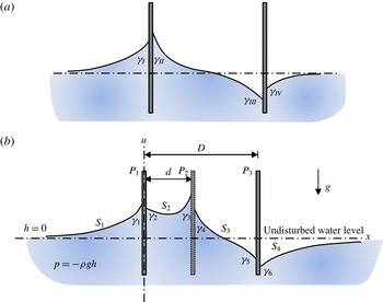
Going back to the capillary interaction, the physics of supported particles is distinctly different from that of particles floating on the water surface, because in the latter case the floating particles are not constrained. To isolate the effect of the capillary interaction, the plate system can be considered where the vertical force and torque balance conditions are neglected. Starov, Velarde & Radke (Reference Starov, Velarde and Radke2007) derived an asymptotic expression of the net horizontal force on the plate in the two-plate system (see figure 1 a) at large separation distances by using the linearization assumption. Results showed that the mutual repulsions can change into attractions between dissimilar plates with the reduction of the separation distance. Finn (Reference Finn2010) studied the net horizontal force on the plate in the two-plate system without the linearization assumption and clarified the behaviours of the configuration, where the Young–Laplace equation reduces to an ordinary differential equation. Recently, the topic has been largely developed in various aspects by a series of researches (Bullard & Garboczi Reference Bullard and Garboczi2009; Bhatnagar & Finn Reference Bhatnagar and Finn2013; Finn Reference Finn2013; Finn & Lu Reference Finn and Lu2013; Aspley, He & McCuan Reference Aspley, He and McCuan2015; Bhatnagar & Finn Reference Bhatnagar and Finn2016b ). For example, more details of the singularity of the horizontal force on the plates are presented in the configuration in which the contact angles on the sides of the plates facing each other are supplements, with the distance of the plates tending to zero (Bhatnagar & Finn Reference Bhatnagar and Finn2016b ). Since the capillary forces in the two-plate system are discussed thoroughly, the question of that in the three-plate system (see figure 1 b) is a natural one. The capillary forces in the three-plate system are analogous to those of brick objects floating on an infinite water bath (Bowden et al. Reference Bowden, Terfort, Carbeck and Whitesides1997) until the menisci reach the edge of the floating brick object. Bowden et al. (Reference Bowden, Terfort, Carbeck and Whitesides1997) studied the configuration using the linearized Young–Laplace equation, which may conceal some remarkable properties at the steep meniscus slope. For example, the non-uniqueness of the equilibria for the middle plate in the three-plate system has not been considered previously.
In this paper, a mathematical model is developed, based on the Young–Laplace equation and retaining its nonlinearity, to calculate the horizontal force of the middle plate in the three-plate system and to characterize its dependence on the combination of contact angles and the distance
 $D$
between the plates on both sides. The study is then extended to determine the qualitative changes of stability and behaviours as the distance
 $D$
varies. The striking properties are related to the bifurcation theory (Seydel Reference Seydel2009), and the distance
 $D$
is chosen as the bifurcation parameter. Once the bifurcation diagrams are determined, the stabilities of equilibria and the behaviour can be obtained with the force profile of the middle plate (Seydel Reference Seydel2009).
Schematics of the two-plate system: (a) two spaced parallel vertical plates partially immersed in an infinite water bath of four distinct materials used for the four surfaces, respectively, and (b) the three-plate system studied in this paper.

2 Model
A mathematical model is proposed to model the horizontal force on the middle plate, which is located between two spaced parallel plates partially immersed in an infinite water bath in a downward gravity field, as indicated in figure 1(b). The plate in the middle (
 $P_{2}$
) can move freely only in the horizontal direction, while the two plates (
 $P_{1}$
and
 $P_{3}$
) with distance
 $D$
between them are stationary. The initial position of plate
 $P_{2}$
is at distance
 $d$
away from plate
 $P_{1}$
. The surfaces of the three plates are constructed of possibly six distinct materials. The contact angle on each face is determined by the material of that face. For simplicity, the thickness of each plate is ignored, which has no effect on the capillary forces.
2.1 Young–Laplace equation in two dimensions
The air–water interfaces
 $S_{2}$
and
 $S_{3}$
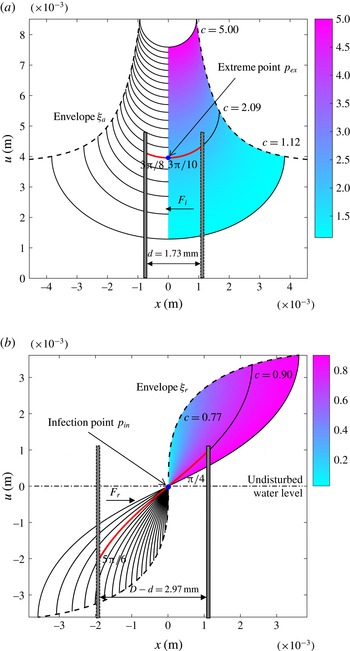
in the three-plate system are the red segments of the solution curves of the Young–Laplace equation in two dimensions, as indicated in figure 2. The behaviours of the solutions of the Young–Laplace equation in two dimensions are discussed thoroughly by Bhatnagar & Finn (Reference Bhatnagar and Finn2016a
). In what follows, the results of that paper are extensively used. The Young–Laplace equation in two dimensions,
 $$\begin{eqnarray}\displaystyle \left(\frac{u_{x}}{\sqrt{1+u_{x}^{2}}}\right)_{x}\equiv \left(\sin \unicode[STIX]{x1D713}\right)_{x}=\unicode[STIX]{x1D705}u, & & \displaystyle\end{eqnarray}$$
describes the height
 $u(x)$
of the water surface, yielding the equilibrium condition for the air–water interface, whose planar curvature is proportional to its height
 $u$
, with the factor
 $\unicode[STIX]{x1D705}$
. In this equation, the subscript
 $x$
represents the derivative with respect to the coordinate
 $x$
(i.e.
 $\bullet _{x}\equiv \text{d}\bullet /\text{d}x$
),
 $\unicode[STIX]{x1D713}$
is the inclination angle of the curve
 $u\left(x\right)$
and
 $\unicode[STIX]{x1D705}=\unicode[STIX]{x1D70C}g/\unicode[STIX]{x1D70E}$
is the capillary constant, with the density difference
 $\unicode[STIX]{x1D70C}$
(positive) between air and water, the gravitational acceleration
 $g$
and the surface tension
 $\unicode[STIX]{x1D70E}$
of the interface.
Two families of solution curves (see also figures 2 and 4 in Bhatnagar & Finn Reference Bhatnagar and Finn2016a
): (a) the attraction family and (b) the repulsion family. In the two families of curves, each curve is cut by the envelope at an inclination angle
 $\unicode[STIX]{x1D713}=\pm \unicode[STIX]{x03C0}/2$
. The red segment in the attraction family represents the water surface
 $S_{2}$
with contact angle pair
 $\left(\unicode[STIX]{x1D6FE}_{2},\unicode[STIX]{x1D6FE}_{3}\right)=\left(3\unicode[STIX]{x03C0}/8,3\unicode[STIX]{x03C0}/10\right)$
and the distance
 $d=1.73~\text{mm}$
between the plates
 $P_{1}$
and
 $P_{2}$
, whereas in the repulsion family the red segment corresponds to
 $S_{3}$
with
 $\left(\unicode[STIX]{x1D6FE}_{4},\unicode[STIX]{x1D6FE}_{5}\right)=\left(5\unicode[STIX]{x03C0}/6,\unicode[STIX]{x03C0}/4\right)$
and
 $D-d=2.97~\text{mm}$
between the plates
 $P_{2}$
and
 $P_{3}$
. The horizontal capillary forces
 $F_{l}$
and
 $F_{r}$
on the left and right surfaces of
 $P_{2}$
depend only on the constants
 $c$
of the water surfaces on the left and right sides of the middle plate, respectively.

There are two methods to obtain the solutions of (2.1). Miersemann (Reference Miersemann2015) obtained the solutions by straight integration of (2.1) while Bhatnagar & Finn (Reference Bhatnagar and Finn2016a
) proposed and then integrated the parametrization form of (2.1) to get the solutions. The solutions could be classified into two families of curves according to the range of the constant of integration
 $c=\unicode[STIX]{x1D705}u^{2}/2+\cos \unicode[STIX]{x1D713}$
and are uniquely determined by the prescribed point
 $(x^{\ast },u^{\ast })$
on the meniscus and the inclination angle
 $\unicode[STIX]{x1D713}^{\ast }$
of the interface at the prescribed point. The right parts of solution curves (colour regions in figure 2) are given parametrically by Bhatnagar & Finn (Reference Bhatnagar and Finn2016a
)
 $$\begin{eqnarray}\displaystyle & \displaystyle c=\frac{\unicode[STIX]{x1D705}}{2}(u^{\ast })^{2}+\cos \unicode[STIX]{x1D713}^{\ast }, & \displaystyle\end{eqnarray}$$
 $$\begin{eqnarray}\displaystyle & \displaystyle x=x^{\ast }+\frac{1}{\sqrt{2\unicode[STIX]{x1D705}}}\int _{\unicode[STIX]{x1D713}^{\ast }}^{\unicode[STIX]{x1D713}}\frac{\cos \unicode[STIX]{x1D70F}\,\text{d}\unicode[STIX]{x1D70F}}{\sqrt{c-\cos \unicode[STIX]{x1D70F}}},\quad \unicode[STIX]{x1D713}\in \left[\unicode[STIX]{x1D713}^{\ast },\frac{\unicode[STIX]{x03C0}}{2}\right], & \displaystyle\end{eqnarray}$$
 $$\begin{eqnarray}\displaystyle & \displaystyle u=\sqrt{\frac{2}{\unicode[STIX]{x1D705}}}\sqrt{c-\cos \unicode[STIX]{x1D713}}. & \displaystyle\end{eqnarray}$$
The elliptic integral involved in the expression of the solutions (2.3) is shown as
 $$\begin{eqnarray}\displaystyle H=\int _{\unicode[STIX]{x1D713}^{\ast }}^{\unicode[STIX]{x1D713}}\frac{\cos \unicode[STIX]{x1D70F}\,\text{d}\unicode[STIX]{x1D70F}}{\sqrt{c-\cos \unicode[STIX]{x1D70F}}}. & & \displaystyle\end{eqnarray}$$
In general, elliptic integrals cannot be expressed in terms of elementary functions. With the appropriate reduction formula, all elliptic integrals can be brought into a form that involves integrals over rational functions and three Legendre canonical forms (i.e. elliptic integrals of the first
 $F$
, second
 $E$
and third
 $\unicode[STIX]{x1D6F1}$
kinds), where the Legendre forms are useful for numerical calculation (Abramowitz & Stegun Reference Abramowitz and Stegun1964). The transformed form of (2.5) is determined by the value of
 $c$
.
In figure 2(a), the solution curves belong to the attraction family of curves, with the value of
 $c$
greater than 1. The meaning of ‘attraction’ is that for the attraction family of curves there are mutual attraction forces in the two-plate system, whereas ‘repulsion’ corresponds to repulsion forces. There are additional solution curves obtained by reflecting the entire configuration with respect to the
 $x$
-axis, yielding an equivalent example with negative height and the same value of
 $c$
. With the increase of the value of
 $c$
, the height and the width of the solution curve increases and decreases, respectively. There is an extreme point
 $p_{ex}$
on each curve in the attraction family. Every solution curve is symmetric with respect to the
 $u$
-axis at the extreme point. Because the inclination angle of the extreme point is zero, the height of the extreme point on the curve of the solution can be calculated by
 $u_{ex}=\pm \sqrt{c-1}$
, whose sign is the same as the sign of the height of the prescribed point. By selecting the extreme point
 $p_{ex}$
as the prescribed point (
 $\unicode[STIX]{x1D713}^{\ast }=0$
), the elliptic integral
 $H$
is given in terms of Legendre forms:
 $$\begin{eqnarray}\displaystyle H=2\sqrt{c+1}\left[E\left(\unicode[STIX]{x1D6FC}_{1},k_{1}\right)-E\left(\frac{\unicode[STIX]{x03C0}}{2},k_{1}\right)\right]-\frac{2c}{\sqrt{c+1}}\left[F\left(\unicode[STIX]{x1D6FC}_{1},k_{1}\right)-F\left(\frac{\unicode[STIX]{x03C0}}{2},k_{1}\right)\right], & & \displaystyle\end{eqnarray}$$
where
 $k_{1}=\sqrt{2/(c+1)}$
is the elliptic modulus and
 $\unicode[STIX]{x1D6FC}_{1}=(\unicode[STIX]{x03C0}-\unicode[STIX]{x1D713})/2$
is the amplitude with
 $\unicode[STIX]{x1D713}\in [0,\unicode[STIX]{x03C0}/2]$
.
When the value of
 $c$
is greater than 0 and less than 1, the solution curves belong to the repulsion family of curves, as shown in figure 2(b). Similar to the attraction family, the additional solution curves can be obtained by reflecting the entire configuration with respect to the
 $x$
-axis. There is no extreme point but an inflection point
 $p_{in}$
on each curve. Every solution curve has point symmetry at the inflection point. The height of the inflection point is zero while the value of the inclination angle at the inflection point is given by
 $\arccos (c)$
. With the increase of the value of
 $c$
, the width of the curve decreases and the inclination angle at the inflection point increases. Selecting the inflection point
 $p_{in}$
as the prescribed point (
 $\unicode[STIX]{x1D713}^{\ast }=\unicode[STIX]{x1D713}_{0}$
), the elliptic integral
 $H$
is given by
 $$\begin{eqnarray}\displaystyle H=2\sqrt{2}\left[E\left(\unicode[STIX]{x1D6FC}_{2},k_{2}\right)-E\left(\frac{\unicode[STIX]{x03C0}}{2},k_{2}\right)\right]-\sqrt{2}\left[F\left(\unicode[STIX]{x1D6FC}_{2},k_{2}\right)-F\left(\frac{\unicode[STIX]{x03C0}}{2},k_{2}\right)\right], & & \displaystyle\end{eqnarray}$$
where
 $$\begin{eqnarray}\displaystyle k_{2}=\cos \frac{\unicode[STIX]{x1D713}_{0}}{2}\quad \text{and}\quad \unicode[STIX]{x1D6FC}_{2}=\arcsin \left(\displaystyle \frac{\cos \displaystyle \frac{\unicode[STIX]{x1D713}}{2}}{\cos \displaystyle \frac{\unicode[STIX]{x1D713}_{0}}{2}}\right)\quad \text{with}~\unicode[STIX]{x1D713}\in [\unicode[STIX]{x1D713}_{0},\unicode[STIX]{x03C0}/2].\qquad & & \displaystyle\end{eqnarray}$$
When the value of
 $c$
is equal to 1, there are four barrier curves separating two families of solution curves. The elliptic integral
 $H$
can be expressed in terms of elementary functions:
 $$\begin{eqnarray}\displaystyle H=2\sqrt{2}\left[\cos \frac{\unicode[STIX]{x1D713}}{2}-\cos \frac{\unicode[STIX]{x1D713}^{\ast }}{2}\right]-\sqrt{2}\left[\ln \left(\frac{\tan \displaystyle \frac{\unicode[STIX]{x1D713}}{4}}{\tan \displaystyle \frac{\unicode[STIX]{x1D713}^{\ast }}{4}}\right)\right]. & & \displaystyle\end{eqnarray}$$
Because of the translation invariance of the solutions in the
 $x$
coordinate and also the reflection invariance in the
 $x$
and
 $u$
coordinates, (2.2), (2.3) and (2.4) can represent all solution curves except for the trivial case
 $u\equiv 0$
, where the elliptic integral
 $H$
in (2.3) can be rewritten as one of (2.6)–(2.9) according to the value of
 $c$
.
2.2 Horizontal forces on the middle plate
The horizontal force in the three-plate system can be calculated by the geometric method (Finn Reference Finn2010) and the energy variation method (McCuan Reference McCuan2007). The net horizontal force
 $F=F_{r}-F_{l}$
(positive direction is to right) on the middle plate is the sum of the horizontal components of the net tension force and the pressure force on the plate arising from the disturbed water. In figure 1(b), the net horizontal force is given in terms of the integral constant
 $c$
(Aspley et al.
Reference Aspley, He and McCuan2015):
 $$\begin{eqnarray}\displaystyle F=\unicode[STIX]{x1D70E}(c_{r}-c_{l}), & & \displaystyle\end{eqnarray}$$
where
 $c_{l}$
and
 $c_{r}$
are the integral constants of the air–water interface on the left and right sides of the middle plate
 $P_{2}$
, respectively.
The three-plate system can be divided into two two-plate systems. For the two-plate system in figure 1(a), the integral constant
 $c$
of the water surface between the plates is determined by the distance between the two plates and the contact angles
 $\unicode[STIX]{x1D6FE}_{II}$
and
 $\unicode[STIX]{x1D6FE}_{III}$
on the inner-facing surfaces of the plates. The horizontal force on a single plate is given by
 $F=\unicode[STIX]{x1D70E}(c-1)$
. Aspley et al. (Reference Aspley, He and McCuan2015) found that, when changing the distance between the plates, the net horizontal force profiles of the two-plate system can be divided into three distinct non-trivial types depending only on the contact angle pair
 $(\unicode[STIX]{x1D6FE}_{II},\unicode[STIX]{x1D6FE}_{III})$
. Similarly, the relation between constant
 $c$
and the distance
 $d$
can be classified into three types according to the contact angle pair
 $(\unicode[STIX]{x1D6FE}_{II},\unicode[STIX]{x1D6FE}_{III})$
.
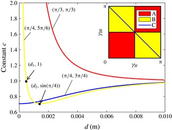
Three types (A, B and C) of curves
 $c(d)$
are shown in figure 3. These curves show distinct characteristics with different pairs of contact angles
 $(\unicode[STIX]{x1D6FE}_{II},\unicode[STIX]{x1D6FE}_{III})$
. In the red region A (i.e. curve
 $c(d)$
belongs to the type A), the value of
 $c$
decreases from infinity to 1 with the increase of
 $d$
as shown by the red typical curve. In the yellow region B, the value of
 $c$
first decreases from infinity to
 $u_{min}=\max (\sin \unicode[STIX]{x1D6FE}_{II},\sin \unicode[STIX]{x1D6FE}_{III})$
and then increases to 1 as shown by the yellow typical curve. On the blue line C, the value of
 $c$
increases from
 $u_{min}=\sin \unicode[STIX]{x1D6FE}_{II}$
to 1 as shown by the blue typical curve. The curves
 $c(d)$
remain unchanged when the pair of contact angles
 $(\unicode[STIX]{x1D6FE}_{II},\unicode[STIX]{x1D6FE}_{III})$
is replaced with the supplementary angles
 $(\unicode[STIX]{x03C0}-\unicode[STIX]{x1D6FE}_{II},\unicode[STIX]{x03C0}-\unicode[STIX]{x1D6FE}_{III})$
, which can be inferred from the reflection invariance of the solutions of the Young–Laplace equation (2.1) in the
 $u$
coordinate.
The inverse function
 $d(c)$
can be calculated by the solutions with the transformed elliptic integral
 $H$
, which is determined by the value of
 $c$
. The integral forms of
 $d(c)$
for different contact angle pairs
 $(\unicode[STIX]{x1D6FE}_{II},\unicode[STIX]{x1D6FE}_{III})$
were given in Finn (Reference Finn2013). In what follows, with the aid of (2.6) and (2.7), the explicit forms of
 $d(c)$
are given in terms of the Legendre forms.
Three types of the curves
 $c(d)$
with different pairs of contact angles
 $(\unicode[STIX]{x1D6FE}_{II},\unicode[STIX]{x1D6FE}_{III})$
.

For the type A in figure 3, assume without loss of generality that
 $(\unicode[STIX]{x1D6FE}_{II},\unicode[STIX]{x1D6FE}_{III})\in [0,\unicode[STIX]{x03C0}/2)\times [0,\unicode[STIX]{x03C0}/2)$
. The inverse function
 $d(c)$
can be given by
 $$\begin{eqnarray}\displaystyle d(c) & = & \displaystyle \sqrt{\frac{2}{\unicode[STIX]{x1D705}}}\left\{\vphantom{\frac{c}{\sqrt{c+1}}}\sqrt{c+1}\left[E\left(\unicode[STIX]{x1D6FC}_{III}^{A},k\right)-E\left(\unicode[STIX]{x1D6FC}_{II}^{A},k\right)\right]\right.\nonumber\\ \displaystyle & & \displaystyle \left.-\,\frac{c}{\sqrt{c+1}}\left[F\left(\unicode[STIX]{x1D6FC}_{III}^{A},k\right)-F\left(\unicode[STIX]{x1D6FC}_{II}^{A},k\right)\right]\right\},\end{eqnarray}$$
where
 $$\begin{eqnarray}\displaystyle \unicode[STIX]{x1D6FC}_{II}^{A}=\frac{3\unicode[STIX]{x03C0}-2\unicode[STIX]{x1D6FE}_{II}}{4},\quad \unicode[STIX]{x1D6FC}_{III}^{A}=\frac{\unicode[STIX]{x03C0}+2\unicode[STIX]{x1D6FE}_{III}}{4}\quad \text{and}\quad k=\sqrt{\frac{2}{c+1}}. & & \displaystyle\end{eqnarray}$$
The case for the type B is more complex because the value of
 $c$
can be either greater or less than one, leading to a piecewise function of
 $c(d)$
. Assume without loss of generality that
 $\sin \unicode[STIX]{x1D6FE}_{II}>\sin \unicode[STIX]{x1D6FE}_{III}$
and
 $(\unicode[STIX]{x1D6FE}_{II},\unicode[STIX]{x1D6FE}_{III})\in (\unicode[STIX]{x03C0}/2,\unicode[STIX]{x03C0}]\times [0,\unicode[STIX]{x03C0}/2)$
. The inverse function
 $d(c)$
can be given as a unified form
 $$\begin{eqnarray}\displaystyle d(c)=\frac{1}{\sqrt{\unicode[STIX]{x1D705}}}\left\{a\left[E\left(\unicode[STIX]{x1D6FC}_{III}^{B},k\right)-E\left(\unicode[STIX]{x1D6FC}_{II}^{B},k\right)\right]-b\left[F\left(\unicode[STIX]{x1D6FC}_{III}^{B},k\right)-F\left(\unicode[STIX]{x1D6FC}_{II}^{B},k\right)\right]\right\}\!, & & \displaystyle\end{eqnarray}$$
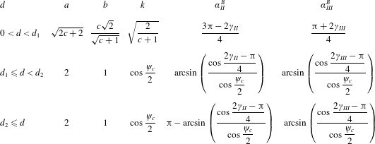
where the parameters are given in table 1.
Parameters in (2.13) for the case of type B:
 $d_{1}=d(1)$
,
 $d_{2}=d(\sin \unicode[STIX]{x1D6FE}_{II})$
,
 $\unicode[STIX]{x1D713}_{c}=\arccos c$
,
 $0<d<d_{1}$
corresponds to
 $1<c$
,
 $d_{1}\leqslant d<d_{2}$
to
 $\sin \unicode[STIX]{x1D6FE}_{II}<c\leqslant 1$
and
 $d_{2}\leqslant d$
to
 $\sin \unicode[STIX]{x1D6FE}_{II}\leqslant c<1$
.

For the type C, assume without loss of generality that
 $\unicode[STIX]{x1D6FE}_{II}\in (\unicode[STIX]{x03C0}/2,\unicode[STIX]{x03C0}]$
. The expression of
 $d(c)$
is the same as the case for
 $d_{2}\leqslant d$
of the type B.
Five distinct types of net horizontal force profiles on the middle plate.

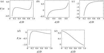
In contrast to the two-plate system, the force profiles of the middle plate
 $P_{2}$
in the three-plate system have more types, which depend only on two contact angle pairs
 $(\unicode[STIX]{x1D6FE}_{2},\unicode[STIX]{x1D6FE}_{3})$
and
 $(\unicode[STIX]{x1D6FE}_{4},\unicode[STIX]{x1D6FE}_{5})$
and the distance
 $D$
. The functions
 $c_{l}\left(d;\unicode[STIX]{x1D6FE}_{2},\unicode[STIX]{x1D6FE}_{3}\right)$
and
 $c_{r}(D-d;\unicode[STIX]{x1D6FE}_{4},\unicode[STIX]{x1D6FE}_{5})$
can be obtained by their inverse functions. Substituting the numerical results into (2.10), the curves of the net horizontal force
 $F(d)$
of the middle plate
 $P_{2}$
can be obtained by
 $$\begin{eqnarray}\displaystyle F\left(d\right)=\unicode[STIX]{x1D70E}\left[c_{r}\left(D-d;\unicode[STIX]{x1D6FE}_{4},\unicode[STIX]{x1D6FE}_{5}\right)-c_{l}\left(d;\unicode[STIX]{x1D6FE}_{2},\unicode[STIX]{x1D6FE}_{3}\right)\right]. & & \displaystyle\end{eqnarray}$$
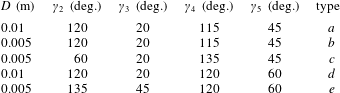
In figure 4, there are five distinct types (a–e) of force profiles
 $F(d)$
for five specific groups of parameter values listed in table 2, which represent the more general situation for the horizontal force on a single plate. In figure 4(a,b), two contact angle pairs are the same and both are located in the regions B–B (i.e.
 $(\unicode[STIX]{x1D6FE}_{2},\unicode[STIX]{x1D6FE}_{3})\in \text{B}$
and
 $(\unicode[STIX]{x1D6FE}_{4},\unicode[STIX]{x1D6FE}_{5})\in \text{B}$
in figure 3), leading to infinite forces at both ends of the curve. In figure 4(c–e), the force profiles have the contact pair
 $(\unicode[STIX]{x1D6FE}_{4},\unicode[STIX]{x1D6FE}_{5})$
belonging to type C, which causes the curves to be limited at the right end. The types of (
 $c$
), (
 $d$
) and (
 $e$
) can degenerate into three types of force profiles in the two-plate system with
 $(\unicode[STIX]{x1D6FE}_{4},\unicode[STIX]{x1D6FE}_{5})=(\unicode[STIX]{x03C0}/2,\unicode[STIX]{x03C0}/2)$
.
Quantities entering into the force equation (2.14).

2.3 Equilibrium of the middle plate
When the horizontal force is equal to zero, the middle plate is in the equilibrium state. All the equilibria could be solved numerically by the equation with the given distance
 $D$
and two pairs of contact angles
 $(\unicode[STIX]{x1D6FE}_{2},\unicode[STIX]{x1D6FE}_{3})$
and
 $(\unicode[STIX]{x1D6FE}_{4},\unicode[STIX]{x1D6FE}_{5})$
:
 $$\begin{eqnarray}\displaystyle c_{l}(d)=c_{r}(D-d). & & \displaystyle\end{eqnarray}$$
Since
 $c(d)$
cannot be written in explicit form, (2.15) is hard to solve. The inverse of the function (2.15) can be given by an explicit form
 $$\begin{eqnarray}\displaystyle d(c;\unicode[STIX]{x1D6FE}_{2},\unicode[STIX]{x1D6FE}_{3})+d(c;\unicode[STIX]{x1D6FE}_{4},\unicode[STIX]{x1D6FE}_{5})=D. & & \displaystyle\end{eqnarray}$$
Since (2.16) in explicit form is expressed in terms of functions (2.11) and (2.13) according to two pairs of contact angles
 $(\unicode[STIX]{x1D6FE}_{2},\unicode[STIX]{x1D6FE}_{3})$
and
 $(\unicode[STIX]{x1D6FE}_{4},\unicode[STIX]{x1D6FE}_{5})$
, (2.16) can be solved by the algorithm ZEROIN for nonlinear equations (Forsythe, Moler & Malcolm Reference Forsythe, Moler and Malcolm1977), which uses a combination of bisection, secant and inverse quadratic interpolation methods. The number of solutions will change as
 $D$
varies. The possible situations are: no solution, one solution, two solutions and three solutions. These situations will be discussed in the next section.
3 Bifurcations of the system
To understand the qualitative behaviours of the three-plate system as the parameters vary, the bifurcation theory (Seydel Reference Seydel2009) is applied for the stability analysis and the prediction of the system behaviours.
3.1 Stability analysis
Suppose the air–water interfaces are in equilibrium and stable and the pressure is hydrostatic in the liquid bath. The energy functional of the system is
 $E(d,D)$
with the prescribed contact angle pairs
 $(\unicode[STIX]{x1D6FE}_{2},\unicode[STIX]{x1D6FE}_{3})$
and
 $(\unicode[STIX]{x1D6FE}_{4},\unicode[STIX]{x1D6FE}_{5})$
. Here the distances
 $d$
and
 $D$
are the parameters of the energy functional. The first variation of
 $E$
with respect to the horizontal motion of the plate
 $P_{2}$
is the net horizontal force
 $F$
on the plate
 $P_{2}$
(Kralchevsky et al.
Reference Kralchevsky, Paunov, Denkov, Ivanov and Nagayama1993)
 $$\begin{eqnarray}\displaystyle -\frac{\unicode[STIX]{x2202}E}{\unicode[STIX]{x2202}d}=F. & & \displaystyle\end{eqnarray}$$
The stabilities of the equilibria are determined by the net horizontal force profiles as shown in figure 4. When
 $\unicode[STIX]{x2202}F/\unicode[STIX]{x2202}d<0$
at the equilibrium point (i.e.
 $\unicode[STIX]{x2202}E/\unicode[STIX]{x2202}d=0,~\unicode[STIX]{x2202}^{2}E/\unicode[STIX]{x2202}d^{2}>0$
), the equilibrium of the middle plate is stable, whereas
 $\unicode[STIX]{x2202}F/\unicode[STIX]{x2202}d>0$
corresponds to the unstable state. However, it is difficult to know the sign of
 $\unicode[STIX]{x2202}F/\unicode[STIX]{x2202}d$
without plotting the force profile in the equilibrium state. An alternative to stability analysis is bifurcation theory. This approach extracts information from the families of equilibria, thereby avoiding calculating
 $\unicode[STIX]{x2202}^{2}E/\unicode[STIX]{x2202}d^{2}$
directly.
Selecting the distance
 $D$
as the bifurcation parameter, the energy functional
 $E(d,D)$
has branches of extremals (i.e. solutions of
 $\unicode[STIX]{x2202}E/\unicode[STIX]{x2202}d=0$
). The dimensionless position
 $d/D$
of
 $P_{2}$
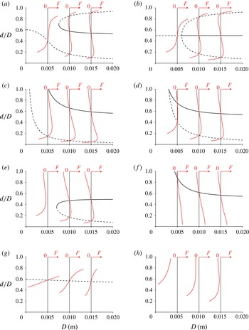
is chosen as the ordinate in the bifurcation diagrams. For different combinations of contact angles, the bifurcation diagrams are determined numerically by solving (2.16) with
 $D$
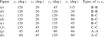
varying, as shown in figure 5. The combinations of contact angles entering (2.16) are listed in table 3.
The combinations of the contact angles in figure 5. The types of
 $c_{l}$
–
 $c_{r}$
are the combination of the types of the curves
 $c(d)$
. For example, the type B–C means that the curves
 $c(d)$
belong to types B and C on the left and right sides of
 $P_{2}$
, respectively.

For the prescribed contact angles, the bifurcation diagram can be determined. The stabilities of branches in the bifurcation diagram can be inferred from the force profile of
 $P_{2}$
. There is no need to obtain all the force profiles as
 $D$
varies. When the stability of one point of equilibria on the branch is determined, the stability of the branch is the same as the stability of this point (Seydel Reference Seydel2009).
In figure 5(a,b), the
 $d/D$
versus
 $D$
diagrams are drawn for the type B–B. Figure 5(b) shows a subcritical pitchfork bifurcation at the point
 $(D,d/D)=(2d_{2},1/2)$
. In this case, for
 $D<2d_{2}$
the equilibrium at
 $d/D=1/2$
is unstable. For
 $D>2d_{2}$
the equilibrium
 $d/D=1/2$
is stable, and there are two unstable equilibria on the two sides. Here
 $d_{2}$
can be calculated by substituting
 $c=\sin (2\unicode[STIX]{x03C0}/3)$
into (2.13). Figure 5(a) shows the symmetry breaking of the pitchfork bifurcation. The dashed curve represents the unstable equilibrium. The upper curve is similar to the fold bifurcation in which one branch is unstable, while the other is stable. Figure 5(c–e) shows diagrams for the type B–C, where one branch is stable and the other is unstable. In figure 5(f,g), there is only one branch of equilibria, and the stabilities of equilibria are determined by the type of
 $c_{l}$
–
 $c_{r}$
. For the type C–C the equilibria are stable while for the type A–A the equilibria are unstable. In figure 5(h), there is no equilibrium for the type A–C. For the type A–B, the diagrams are not drawn, as they are the same as the diagrams for the type A–A in qualitative sense. Additional diagrams can be obtained by reflecting the bifurcation diagrams with respect to the horizontal line
 $d/D=1/2$
, which belong to the mirror image cases of the original three-plate systems.
The bifurcation diagrams for
 $d/D$
versus
 $D$
. The solid curve denotes the branch of the stable equilibria while the dashed curve corresponds to the unstable equilibria. The red curve represents the horizontal force profile
 $F(d/D)$
on the plate
 $P_{2}$
.

In figure 5(a–e), the factors affecting the bifurcation diagram qualitatively include not only the types of
 $c_{l}$
–
 $c_{r}$
but also the values of
 $\sin \unicode[STIX]{x1D6FE}_{2}$
and
 $\sin \unicode[STIX]{x1D6FE}_{4}$
. In these cases, the contact angles are deliberately given with
 $\sin \unicode[STIX]{x1D6FE}_{2}\geqslant \sin \unicode[STIX]{x1D6FE}_{3}$
and
 $\sin \unicode[STIX]{x1D6FE}_{4}\geqslant \sin \unicode[STIX]{x1D6FE}_{5}$
without the change of the curves
 $c_{l}(d)$
and
 $c_{r}(D-d)$
. In figure 5(a), the values of
 $\sin \unicode[STIX]{x1D6FE}_{2}$
and
 $\sin \unicode[STIX]{x1D6FE}_{4}$
are not equal, which causes the symmetry breaking of the pitchfork bifurcation. In figure 5(b), the relation
 $\sin \unicode[STIX]{x1D6FE}_{2}=\sin \unicode[STIX]{x1D6FE}_{4}$
leads to the pitchfork bifurcation diagram. For the case of the type B–C, the relation between
 $\sin \unicode[STIX]{x1D6FE}_{2}$
and
 $\sin \unicode[STIX]{x1D6FE}_{4}$
determines the shape of the diagram. When
 $\sin \unicode[STIX]{x1D6FE}_{2}<\sin \unicode[STIX]{x1D6FE}_{4}$
, the diagram shows two disjoint branches of the equilibria as shown in figure 5(c), whereas
 $\sin \unicode[STIX]{x1D6FE}_{2}>\sin \unicode[STIX]{x1D6FE}_{4}$
corresponds to one curve (i.e. the fold bifurcation) of the equilibria as shown in figure 5(e). The diagram with
 $\sin \unicode[STIX]{x1D6FE}_{2}=\sin \unicode[STIX]{x1D6FE}_{4}$
in figure 5(d) is the transitional state of the diagrams in figure 5(c,e).
3.2 Behaviour prediction of the system
Under the lateral forces, the plate
 $P_{2}$
will be either attracted to any stationary plate (
 $P_{1}$
or
 $P_{3}$
) or stay at an equilibrium position (stable) near the centre between the two stationary plates. Once the bifurcation diagram is determined, the behaviours of the plate
 $P_{2}$
can be predicted with the quasi-static assumption (the water surfaces are in equilibrium when
 $P_{2}$
moves towards the direction of the horizontal force, i.e.
 $P_{2}$
moves at a very slow speed and the forces related to velocity are ignored). The behaviours of the plate
 $P_{2}$
depend on its initial position and the distance
 $D$
. The plate
 $P_{2}$
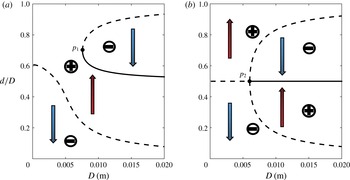
will move in the direction of the arrow (see figure 6) from its initial position.
Two bifurcation diagrams for the type B–B. The red (upward-pointing) and blue (downward-pointing) arrows represent the positive and negative regions, respectively, where the signs represent the signs of the horizontal force
 $F$
on the plate
 $P_{2}$
. The points
 $p_{1}$
and
 $p_{2}$
are the bifurcation points in the diagram.

In figure 6, the bifurcation occurs when a small smooth change made to the value of
 $D$
(the bifurcation parameter) of the system causes a sudden qualitative change in its behaviours at the bifurcation points
 $p_{1}$
and
 $p_{2}$
. For example, when
 $D$
increases by a small value across the point
 $p_{2}$
in figure 6(b), an unstable equilibrium of the plate
 $P_{2}$
turns into a stable equilibrium and two unstable equilibria on the sides.
4 Conclusions
In this paper, the force profiles of the middle plate in the three-plate system are presented with the prescribed quantities: the distance
 $D$
and two pairs of contact angles
 $(\unicode[STIX]{x1D6FE}_{2},\unicode[STIX]{x1D6FE}_{3})$
and
 $(\unicode[STIX]{x1D6FE}_{4},\unicode[STIX]{x1D6FE}_{5})$
. The contact angles are deliberately given with
 $\sin \unicode[STIX]{x1D6FE}_{2}\geqslant \sin \unicode[STIX]{x1D6FE}_{3}$
and
 $\sin \unicode[STIX]{x1D6FE}_{4}\geqslant \sin \unicode[STIX]{x1D6FE}_{5}$
. Various bifurcation diagrams are presented with different combinations of contact angles. The conclusions drawn are as follows.
-
(i) As the middle plate forming the menisci on both sides is moved horizontally the force on the plate depends only on the integral constants (
 $c_{l}$
and
$c_{r}$
) of the water surfaces (
$S_{2}$
and
$S_{3}$
). By changing the distance
$D$
, the number and the position of equilibria (stable and unstable) of the plate
$P_{2}$
can change.
-
(ii) In contrast to the two-plate system, the force profiles are more complicated, and there are five types of force profiles in a three-plate system, three of which are similar to the force profiles of the two-plate system.
-
(iii) The bifurcation diagrams are determined in qualitative sense by the type of
$c_{l}$
–
$c_{r}$
and the relation between
$\sin \unicode[STIX]{x1D6FE}_{2}$
and
$\sin \unicode[STIX]{x1D6FE}_{4}$
, e.g. for the type B–B with
$\sin \unicode[STIX]{x1D6FE}_{2}=\sin \unicode[STIX]{x1D6FE}_{4}$
the bifurcation diagram is a subcritical pitchfork bifurcation. For given quantities, there are at most eight possible diagrams in the three-plate system. -
(iv) The stabilities of equilibria can be obtained by the bifurcation diagram with several force profiles. The branch of the diagram is of the same stability as that of the point on this branch (Seydel Reference Seydel2009). The stability of a point can be inferred from the slope of the force profile. For example, the equilibrium is unstable when the slope at the equilibrium is greater than zero.
-
(v) The behaviours of the plate
$P_{2}$
can be predicted with the quasi-static assumption in diagrams. The plate
$P_{2}$
moves towards the direction of the arrow, which is determined by the sign of the force. The middle plate will eventually move to either the stable equilibrium position or the plates on both sides, which depends on its initial position and the bifurcation diagram.


Acknowledgements
This research was partly supported by the National Natural Science Foundation of China (No. 11672116), the Fundamental Research Funds for the Central Universities, HUST (No. 2015MS057) and the Research Funds from the Hubei Key Laboratory for Engineering Structural Analysis and Safety Assessment.