






1 Introduction
Gravity currents are flows generated by horizontal pressure gradients, as a result of gravity over fluids with different density. This driving effect is also referred to as (horizontal) buoyancy. These flows manifest as a mostly horizontal current of light fluid above a heavy fluid, or as a current of heavy fluid below light fluid. Gravity currents are present in nature and the environment in many situations, such as volcanic clouds, oil leaks in the sea, discharge of gases from exhaust devices, and sand storms in the desert. These phenomena play an important role in the transport of mass, momentum and energy. This was, for instance, recently confirmed in the case of river discharges by Clarke (Reference Clarke2016) who made detailed observations of field-scale turbidity currents sloping off the mouth of the Squamish River (British Columbia, Canada) that discharges more than 1 million cubic metres of sediment per year (Hickin Reference Hickin1989). In particular, these gravity currents, composed of sediment transported as a suspension, can be responsible for massive sediment deposits on the submarine floor of up to few metres, as in the region close to the transition from Agadir Canyon to Agadir Basin, for example (Cantero et al. Reference Cantero, Cantelli, Pirmez, Balachandar, Mohrig, Hickson, Yeh, Naruse and Parker2012).
Allen (Reference Allen1971) and Simpson (Reference Simpson1972) are seminal works that studied the three-dimensional (3-D) structure and dynamics of the front of planar gravity currents and in particular the processes at the origin of the formation of lobes and clefts. The works of Fannelop & Waldman (Reference Fannelop and Waldman1971), Hoult (Reference Hoult1972) and Huppert & Simpson (Reference Huppert and Simpson1980) characterized the dynamics of gravity currents by laboratory experiments and theoretical models, where the different phases of spreading of gravity currents were analysed and scaling laws for the slumping and self-similar regimes were proposed. Mixing in gravity currents has been measured and modelled by Simpson & Britter (Reference Simpson and Britter1979), García & Parsons (Reference García and Parsons1996) and Parsons & García (Reference Parsons and García1998), while the internal structure of gravity fronts has been studied through local measurements of the velocity field by Alahyari & Longmire (Reference Alahyari and Longmire1996) and Patterson et al. (Reference Patterson, Simpson, Dalziel and van Heijst2006). The theoretical understanding, interpretation and approximate prediction of the the gravity current phenomenon is by means of simplified theoretical models; see Ungarish (Reference Ungarish2009). More recently, resolved 3D simulations of non-rotating gravity currents have been performed, for example, by Härtel, Meiburg & Necker (Reference Härtel, Meiburg and Necker2000) and Cantero et al. (Reference Cantero, Lee, Balachandar and García2007b , Reference Cantero, Balachandar, García and Bock2008). These works allowed a full characterization of the flow inside a gravity current and in particular at the front, and an assessment of the relevance of available models predicting the front velocity in all regimes.
At geophysical scales, gravity currents play an important role in river outflows, the circulation of the atmosphere and hydrosphere, and hazards such as volcanic clouds (Griffiths Reference Griffiths1986). In these cases the rotation of the planet may affect the flow field. The typical centrifugal acceleration
 $\unicode[STIX]{x1D6FA}^{2}L$
is insignificant compared to the acceleration due to gravity
 $g$
even for length scales
 $L$
of the order of the Earth’s radius, but the Coriolis acceleration may become the dominant balance of the driving buoyancy effect in a sufficiently long process (typically, a quarter revolution of the system). It is therefore of both theoretical and practical interest to investigate the influence of the Coriolis effect on gravity currents. The rotational effects are accounted for by the ratio between the inertial time scale and the rotational time scale. This ratio is called the Coriolis number
 ${\mathcal{C}}$
(defined in § 2) and can be also related to the Rossby number
 $Ro\sim 1/{\mathcal{C}}$
. Note that when density stratification and rotation are present in the system, as in the present case, one can equivalently define a Burger number
 $Bu$
which is related to the Coriolis number
 $Bu\sim 1/{\mathcal{C}}^{2}$
(see Stegner, Bouruet-Aubertot & Pichon Reference Stegner, Bouruet-Aubertot and Pichon2004). Given the ‘slow’
 $\unicode[STIX]{x1D6FA}\sim 10^{-4}~\text{s}^{-1}$
of the planet, gravity currents in nature are expected to display small
 ${\mathcal{C}}$
. We shall subsequently consider flows with
 ${\mathcal{C}}<1$
(unless stated otherwise).
A great deal of attention has been focused on gravity currents of fixed volume released from a cylinder lock whose axis
 $z$
is parallel to the axis of rotation and antiparallel to gravity (Verzicco, Lalli & Campana Reference Verzicco, Lalli and Campana1997; Hallworth, Huppert & Ungarish Reference Hallworth, Huppert and Ungarish2001; Stegner et al.
Reference Stegner, Bouruet-Aubertot and Pichon2004; Stuart, Sundermeyer & Hebert Reference Stuart, Sundermeyer and Hebert2011; Dai & Wu Reference Dai and Wu2016, Reference Dai and Wu2018). The current spreads out along the radius
 $r$
in an axisymmetric pattern, attains a maximum value
 $r_{max}$
, then performs oscillations. This process, referred to as geostrophic adjustment, occurs in about a quarter revolution of the system. The dense fluid attains a quasi-steady motion with profile
 $h\sim (r_{max}^{2}-r^{2})$
and a significant negative angular velocity parallel to the front (in the rotating system) referred to as transverse anticyclonic velocity; this structure is called a ‘lens’ (see Ungarish Reference Ungarish2009, chap. 8 and the references therein). It is worth noting that in most of the above-mentioned works, the value of the Coriolis number is generally such that
 ${\mathcal{C}}\geqslant 1$
.
In this work we address the counterpart Cartesian problem: the gravity current is ‘planar’ (not cylindrical), released from a rectangular lock, in a rotating system. The motion is not restricted by geometrical obstacles in the forward (streamwise) and lateral (sidewise) directions
 $x$
and
 $y$
, respectively. We thus expect a close (but not perfect) counterpart to the axisymmetric current and lens. The Coriolis effects will stop the
 $x$
propagation at some
 $x_{max}$
, while producing a significant anticyclonic (lateral) velocity. Again, the geostrophic adjustment is expected to produce a quasi-steady profile in the
 $xz$
plane, supported by a sidewise velocity. This counterpart of the lens, which we call a ‘wedge’ due to the shape, will be presented later. The objective of this paper is to study this flow in some detail. To this end, we combine direct numerical simulations (DNS) with a theoretical model. Choosing such a configuration, in contrast to a cylindrical release, allows us to perform a parametric study in the parameter space defined by
 ${\mathcal{C}}$
,
 $Sc$
and the type of top–bottom boundary conditions. In addition, we argue that the present planar configuration is a more relevant set-up for geophysical situations. The typical current is released from a reservoir (lock) which is far away from the axis of rotation. In these circumstances the curvature terms are negligibly small. The planar set-up is not only a simplification, but also highlights the difference between a situation influenced by curvature terms and one which is not.
Firstly, we report on eight 3-D DNS of various boundary conditions (free-slip and no-slip), Schmidt numbers and Coriolis numbers. For this we employ two numerical approaches: a fully de-aliased pseudo-spectral method for simulations with small Schmidt numbers (Canuto et al. Reference Canuto, Hussaini, Quarteroni and Zang1988; Salinas, Cantero & Dari Reference Salinas, Cantero and Dari2014); and a finite-volume/volume-of-fluid method with no interface reconstruction for high Schmidt numbers (Bonometti & Magnaudet Reference Bonometti and Magnaudet2007).
Secondly, the DNS results are compared to the predictions of a theoretical model. In contrast to the high accuracy and detailed flow-field information supplied by the DNS simulations, the theoretical model is concerned with the global behaviour of the current: shape of the interface (assumed sharp), position of the nose-front, and the depth-averaged velocities. This provides insights and estimates concerning the time of formation, spread-out, and magnitude of the anticyclonic velocity. In particular, we show that this theoretical model sheds light on a topic of interest which received little attention in previous investigation is: what happens after the adjustment stage? The dense fluid of the lens, or wedge, is in differential rotation with respect to the ambient. Assuming a stable situation, thin viscous Ekman layers will appear on the boundaries of the dense fluid together with some mixing and entrainment in the interfacial region, and attempt to cancel the lateral speed difference (the so-called spin-up effect). The important by-product is a slow expansion (over many revolutions of the system) of the quasi-steady wedge.
A forerunner to the present investigation was done by Hunt et al. (Reference Hunt, Pacheco, Mahalov and Fernando2005). Briefly, these authors performed 2-D numerical simulations of the Euler equations to investigate the effect of rotation on the dynamics of the front, up to a time corresponding to the first oscillation of the front. They also performed a theoretical analysis of the front shape and dynamics of gravity currents propagating on a slope in a rotating system. Finally, they solved a system of 2-D shallow-water equations, including bottom friction, in order to investigate the front dynamics (in the horizontal case) during the oscillating regime. The model allowed them to observe a slow expansion of the oscillating front, which they attribute to the presence of bottom friction. Note that their work considered a range of Coriolis number of about
 $0.75\leqslant {\mathcal{C}}\leqslant 1.5$
.
The present work extends Hunt et al.’s (Reference Hunt, Pacheco, Mahalov and Fernando2005) results in many ways. Firstly, the present 3-D DNS include viscous effects and thus fully capture the Ekman layers. In addition, the present DNS are performed for much longer times than those reported before. Secondly, we here consider a different range of Coriolis numbers and a large range of Schmidt numbers and top–bottom boundary conditions. Finally, the present theoretical model explicitly accounts for the influence of Ekman layers or mixing at the interface between the current and the ambient and, inter alia, provides theoretical predictions for the geostrophic structure and for the slow expansion of the oscillating front which can be directly compared to the present DNS results.
The paper is structured as follows. We present in § 2 the set of equations and the numerical set-ups used in the DNS. The theoretical model based on shallow-water and Ekman layer spin-up theories is described in § 3. In § 4, we describe the dynamics of rotating gravity currents (
 ${\mathcal{C}}<1$
) obtained from DNS and the present theoretical model. In particular, we follow the ‘chronology’ of the current’s front: early times of propagation until the first arrest; oscillations; slow drift. For each sequence of the dynamics, we present the influence of
 ${\mathcal{C}}$
,
 $Sc$
and the type of top–bottom boundary conditions. Concluding remarks are given in § 5.
2 Mathematical formulation and numerical set-up
2.1 Equations and assumptions
The system under consideration is depicted schematically in figure 1.
Schematic of the configuration considered here. Computational domain used in the present work for the spectral code. For computational reasons, periodic boundary conditions are used along the
 $x$
- and
 $y$
-directions so the heavy fluid is mirrored at the centre of the domain. The heavy fluid is initially located in a box of dimensions
 $x_{0}\times W\times H$
.

In the region
 $0\leqslant x\leqslant x_{0}$
the domain is filled with a fixed volume of heavy fluid of density
 $\unicode[STIX]{x1D70C}_{1}$
and height
 $h_{0}$
(shaded region in figure 1) which is released into an ambient fluid initially of density
 $\unicode[STIX]{x1D70C}_{0}$
and height
 $H$
.
We use a rectangular computational box of size
 $L\times W\times H$
in rotation at an angular velocity
 $\unicode[STIX]{x1D6FA}$
about the vertical axis
 $z$
anti-parallel to gravity.
The density difference between the current and the ambient is small enough that the Boussinesq approximation is valid. In these circumstances the flow is governed by the dimensionless equations
 $$\begin{eqnarray}\displaystyle & \displaystyle \frac{\unicode[STIX]{x2202}\tilde{\boldsymbol{u}}}{\unicode[STIX]{x2202}\tilde{t}}+\tilde{\boldsymbol{u}}\boldsymbol{\cdot }\tilde{\unicode[STIX]{x1D735}}\tilde{\boldsymbol{u}}=-\tilde{\unicode[STIX]{x1D735}}\tilde{p}+\frac{1}{Re}\tilde{\unicode[STIX]{x1D6FB}}^{2}\tilde{\boldsymbol{u}}-\tilde{\unicode[STIX]{x1D70C}}\,\hat{\boldsymbol{z}}-2{\mathcal{C}}(\tilde{u} \hat{\boldsymbol{y}}-\tilde{v}\hat{\boldsymbol{x}}), & \displaystyle\end{eqnarray}$$
 $$\begin{eqnarray}\displaystyle & \displaystyle \tilde{\unicode[STIX]{x1D735}}\boldsymbol{\cdot }\tilde{\boldsymbol{u}}=0, & \displaystyle\end{eqnarray}$$
 $$\begin{eqnarray}\displaystyle & \displaystyle \displaystyle \frac{\unicode[STIX]{x2202}\tilde{\unicode[STIX]{x1D70C}}}{\unicode[STIX]{x2202}\tilde{t}}+\tilde{\boldsymbol{u}}\boldsymbol{\cdot }\tilde{\unicode[STIX]{x1D735}}\tilde{\unicode[STIX]{x1D70C}}=\frac{1}{Re\,Sc}\,\tilde{\unicode[STIX]{x1D6FB}}^{2}\tilde{\unicode[STIX]{x1D70C}}. & \displaystyle\end{eqnarray}$$
Here a tilde (
 ${\sim}$
) denotes a dimensionless quantity,
 $\tilde{\boldsymbol{u}}=\{\tilde{u} ,\tilde{v},\tilde{w}\}$
is the velocity,
 $\tilde{p}$
the pressure, and
 $\tilde{\unicode[STIX]{x1D70C}}$
the density. The scales employed are the current height
 $h_{0}$
as length scale,
 $U=\sqrt{g^{\prime }h_{0}}$
as velocity scale with
 $g^{\prime }=g(\unicode[STIX]{x1D70C}_{1}-\unicode[STIX]{x1D70C}_{0})/\unicode[STIX]{x1D70C}_{0}$
being the reduced gravity,
 $\unicode[STIX]{x1D70C}_{0}U^{2}$
as pressure scale, and
 $T=h_{0}/U$
as time scale. The dimensionless density is given by
 $$\begin{eqnarray}\displaystyle \tilde{\unicode[STIX]{x1D70C}}=\frac{\unicode[STIX]{x1D70C}-\unicode[STIX]{x1D70C}_{0}}{\unicode[STIX]{x1D70C}_{1}-\unicode[STIX]{x1D70C}_{0}}.\end{eqnarray}$$
The dimensionless parameters in (2.1)–(2.3) are the Reynolds, Schmidt, and Coriolis numbers defined as
 $$\begin{eqnarray}Re=\frac{Uh_{0}}{\unicode[STIX]{x1D708}},\quad Sc=\frac{\unicode[STIX]{x1D708}}{\unicode[STIX]{x1D705}},\quad {\mathcal{C}}=\frac{\unicode[STIX]{x1D6FA}h_{0}}{U},\end{eqnarray}$$
where
 $\unicode[STIX]{x1D708}$
is the kinematic viscosity assumed identical for both the current and the ambient,
 $\unicode[STIX]{x1D705}$
the mass diffusivity of the agent responsible for the density contrast, and
 $\unicode[STIX]{x1D734}=\{0,0,\unicode[STIX]{x1D6FA}\}$
is the constant angular velocity of the rotating system. Two other useful dimensionless numbers follow, namely, the Rossby number
 $Ro=1/2{\mathcal{C}}$
, and the Ekman number
 $E=\unicode[STIX]{x1D708}/(\unicode[STIX]{x1D6FA}h_{0}^{2})=({\mathcal{C}}Re)^{-1}$
.
The initial conditions at
 $\tilde{t}=0$
are a release from rest (in the rotating system), in particular
 $\tilde{u} =\tilde{v}=0$
for the dense fluid in the lock. Note that the subsequent motion in the
 $\tilde{x}>0$
and
 ${\tilde{y}}$
-direction is not restricted.
2.2 The two numerical approaches
In this work two different numerical techniques are used: a fully de-aliased pseudo-spectral code (Canuto et al.
Reference Canuto, Hussaini, Quarteroni and Zang1988; Salinas et al.
Reference Salinas, Cantero and Dari2014) and a finite-volume/volume-of-fluid method with no interface reconstruction (Bonometti & Magnaudet Reference Bonometti and Magnaudet2007). The spectral code is used to simulate currents with moderate Schmidt numbers (
 $1\leqslant Sc\leqslant 5$
) while the finite-volume code is used for high-Sc (
 $Sc\rightarrow \infty$
). This allows us to investigate the possible effect of the Schmidt number on the results. In addition, the Reynolds number is set here to 4000.
The computational domain is taken to be long enough along the streamwise direction to allow free unhindered development of the current for a long time according to analytical estimates. Periodic boundary conditions are employed along the spanwise
 $({\tilde{y}})$
-directions, no-slip or free-slip boundary conditions for the velocity and a zero normal gradient condition for the density are used along the vertical
 $(\tilde{z})$
-direction, while a periodic and free-slip boundary condition is used along the streamwise
 $(\tilde{x})$
-direction for the spectral and finite-volume codes, respectively.
The set of Navier–Stokes simulations performed in this work are presented in table 1. Eight cases with different Coriolis numbers (
 $0.1\leqslant {\mathcal{C}}\leqslant 0.25$
), Schmidt numbers (
 $1\leqslant Sc<\infty$
), and boundary conditions at the top and bottom walls (no-slip versus free-slip) are analysed.
Parameters used in the present direct numerical simulations. Each run is denoted by an acronym suggesting the value of the Schmidt number
 $Sc$
(S1, S5, SI for infinite Schmidt), Coriolis number
 ${\mathcal{C}}$
(C10, C15, C25) and the type of top–bottom boundary condition
 $BC$
(N for no-slip, F for free-slip).
 $Ro$
denotes the Rossby number
 $Ro=1/2{\mathcal{C}}$
. PS and FV refer to the pseudo-spectral code and the finite-volume code, respectively.
 $N_{x}$
,
 $N_{y}$
and
 $N_{z}$
are the total number of grid cells and grid points in each direction for the FV and PS codes, respectively. The computational domain size is
 $L\times W\times H$
with
 $W=H=1$
(recall that the domain length is
 $2L$
for the spectral code).
 $FS$
and
 $NS$
refer to free-slip and no-slip, respectively. The table also shows the value of the first maximum distance attained by the propagating front
 $\overline{x}_{max}$
and the corresponding time
 $\tilde{t}_{max}$
.
 $\tilde{T}_{p}$
is the period of the subsequent front oscillations,
 $\overline{\unicode[STIX]{x1D714}}_{p}=2\unicode[STIX]{x03C0}/\overline{T}_{p}$
is the pulse frequency and
 $f=2{\mathcal{C}}$
is the Coriolis parameter of the inertial waves. In all cases, the Reynolds number is
 $Re=4000$
.

2.2.1 Spectral code
Equations (2.1)–(2.3) are solved employing a fully de-aliased pseudo-spectral code (Canuto et al.
Reference Canuto, Hussaini, Quarteroni and Zang1988; Salinas et al.
Reference Salinas, Cantero and Dari2014). The code uses Fourier expansions for the flow variables along the horizontal directions (
 $\tilde{x}$
and
 ${\tilde{y}}$
), while a Chebyshev expansion with Gauss–Lobatto quadrature points is used for the inhomogeneous vertical direction (
 $\tilde{z}$
). The flow field is time-advanced using a Crank–Nicolson scheme for the diffusive terms. The advection terms are handled with the Arakawa method (Durran Reference Durran1999) and advanced with a third-order Runge–Kutta scheme. The buoyancy term is also advanced with a third-order Runge–Kutta scheme.
Detailed implementation of the code can be found in Cantero et al. (Reference Cantero, Balachandar, García and Ferry2006), and validation in the case of non-rotating cylindrical and planar configurations can be found in Cantero, Balachandar & García (Reference Cantero, Balachandar and García2007a ) and Cantero et al. (Reference Cantero, Lee, Balachandar and García2007b ), respectively. In addition, the present pseudo-spectral code has been recently used to simulate rotating gravity currents in a cylindrical configuration (Salinas et al. Reference Salinas, Cantero, Dari and Bonometti2018). In particular, a detailed comparison between the simulations and the experimental results of Hallworth et al. (Reference Hallworth, Huppert and Ungarish2001) was performed and shows reasonable agreement (see Salinas et al. Reference Salinas, Cantero, Dari and Bonometti2018, figures 3–5).
2.2.2 Finite-volume code
The second numerical technique is a finite-volume/volume-of-fluid method with no interface reconstruction. Equations (2.1)–(2.3) are solved using the JADIM code originally developed for two-phase flows with high density ratios (Bonometti & Magnaudet Reference Bonometti and Magnaudet2007). In this approach, we assume the Péclet number (
 $Pe=Re\,Sc$
) to be infinite, that is, (2.3) is chosen to be hyperbolic as the right-hand side is zero. The transport equation of the density is solved using a modified version of the transport scheme proposed by Zalesak (Reference Zalesak1979). Although no physical diffusivity is introduced in the advection of the density, the numerical thickness of the interface is not strictly zero as it is typically resolved over three grid cells. An effective Péclet number can be estimated, which depends on the degree of spatial resolution. The effective Péclet number for the spatial resolution used here is estimated to be of
 $O(10^{5})$
; see the appendix of Bonometti & Balachandar (Reference Bonometti and Balachandar2008) for more details.
The overall algorithm is second-order accurate in both time and space. Details on the algorithms as well as validation of the code may be found in Bonometti, Balachandar & Magnaudet (Reference Bonometti, Balachandar and Magnaudet2008). Note that the computational domain used with the finite-volume code is only half that used for the spectral code (i.e. the domain length is
 $L$
).
A convergence study of the present finite-volume code can be found in Bonometti & Balachandar (Reference Bonometti and Balachandar2008) in the case of non-rotating planar gravity currents (their figures 2–4 and table 1). In addition, a comparison of the dynamics of high Reynolds Boussinesq non-rotating planar gravity currents obtained with the present spectral and finite-volume approaches has been done in this paper and shows that even though the two methods are different, they give very similar results (see their figures 6a and 13 for a comparison of the instantaneous density distribution and time evolution of the front velocity, respectively).
3 The global-flow theoretical model
For insights and comparison we use an approximate theory which we call the shallow-water (SW) model. There is good evidence (see, for example, Ungarish Reference Ungarish2009, § 8.1) that for the axisymmetric case the SW theory predicts well the propagation and the formation of the quasi-steady lens structure. Here we extend the analysis to the present geometry, which can be referred to as a 2.5-D approximation: the current is represented by the
 $h(x,t)$
profile, and the main propagation is given by
 $u(x,t)$
. We assume that the flow is independent of the lateral direction
 $y$
, while there is significant lateral velocity
 $v(x,t)$
(and angular velocity
 $v(x,t)/x$
). This corresponds to the
 $h(r,t)$
,
 $u(r,t)$
,
 $v(r,t)$
description of the axisymmetric current, and the 2.5 dimensions express this similarity. The flow is not 2-D because the lateral momentum balance must be taken into account, but is also is not fully 3-D since the value of the
 $y$
-coordinate does not influence the flow; and hence the 2.5-D designation is applied.
3.1 The balance equations
The SW equations are an extension of those derived for the axisymmetric case (Ungarish Reference Ungarish2009, § 8.1). The main approximations are that the current is a thin layer, the return flow in the ambient is negligible,
 $Re$
is large, and there are no mixing/entrainment effects. In the cases considered here these assumptions are satisfied, at least during the formation motion. In this theoretical model we use the
 $z$
-averaged
 $u$
,
 $v$
. Note that for clarity, and from here on, we remove the tilde from the dimensionless quantities. Because the current is a thin layer, the
 $z$
-acceleration terms are very small and the vertical momentum equations reduce to the hydrostatic balance. Consequently, the pressure-driving (buoyancy) term is given by
 $(\unicode[STIX]{x2202}h/\unicode[STIX]{x2202}x)\hat{x}$
, with
 $\hat{x}$
the unit vector pointing in the
 $x$
-direction. We recall that the variables do not depend on
 $y$
, therefore
 $\unicode[STIX]{x2202}/\unicode[STIX]{x2202}y=0$
and there is no lateral buoyancy-driving.
The equations of continuity, and momentum in the
 $x$
- and
 $y$
-directions, are
 $$\begin{eqnarray}\displaystyle \displaystyle \frac{\unicode[STIX]{x2202}h}{\unicode[STIX]{x2202}t}+u\frac{\unicode[STIX]{x2202}h}{\unicode[STIX]{x2202}x}+h\frac{\unicode[STIX]{x2202}u}{\unicode[STIX]{x2202}x} & =0, & \displaystyle\end{eqnarray}$$
 $$\begin{eqnarray}\displaystyle \displaystyle \frac{\unicode[STIX]{x2202}u}{\unicode[STIX]{x2202}t}+\frac{\unicode[STIX]{x2202}h}{\unicode[STIX]{x2202}x}+u\frac{\unicode[STIX]{x2202}u}{\unicode[STIX]{x2202}x} & =2{\mathcal{C}}v, & \displaystyle\end{eqnarray}$$
 $$\begin{eqnarray}\displaystyle \displaystyle \frac{\unicode[STIX]{x2202}v}{\unicode[STIX]{x2202}t}+u\frac{\unicode[STIX]{x2202}v}{\unicode[STIX]{x2202}x} & =-2{\mathcal{C}}u. & \displaystyle\end{eqnarray}$$
The terms
 $2{\mathcal{C}}v$
and
 $-2{\mathcal{C}}u$
stem from the Coriolis force.
Manipulation of the system (3.1)–(3.3) produces the potential–vorticity conservation equation
 $$\begin{eqnarray}\frac{\text{D}}{\text{D}t}\frac{2{\mathcal{C}}+\unicode[STIX]{x2202}v/\unicode[STIX]{x2202}x}{h}=0,\end{eqnarray}$$
where
 $\text{D}\cdot /\text{D}t=\unicode[STIX]{x2202}\cdot /\unicode[STIX]{x2202}t+u\unicode[STIX]{x2202}\cdot /\unicode[STIX]{x2202}x$
is the material derivative.
The initial conditions employed are a release from rest
 $u=v=0$
from the lock
 $h=1$
,
 $0\leqslant x\leqslant x_{0}$
. The boundary conditions are
 $u=v=0$
at the wall
 $x=0$
, and at the nose
 $$\begin{eqnarray}u_{N}=Fr\sqrt{h},\quad v_{N}=-2{\mathcal{C}}(x_{N}-x_{0}).\end{eqnarray}$$
Equation (3.5) is the standard Benjamin-like propagation jump condition, and we use the Huppert–Simpson
 $Fr=1.19$
estimate. Equation (3.5) is angular momentum conservation on the front. It can be obtained by the integration of (3.3) on the characteristic from
 $x=x_{0}$
where
 $v=0$
. An auxiliary condition is the conservation of total volume (
 $=x_{0}$
in dimensionless form). The system of equations is hyperbolic, and can be solved numerically as explained in Ungarish (Reference Ungarish2009). A typical feature of the solution, for all tested cases, is that the current attains a maximum spread,
 $x_{max}$
, in a fairly short time. In this situation, while
 $u=0$
at the nose, a negative
 $u$
is present in the current, which indicates the beginning of a contraction.
3.2 Steady-state ‘wedge’ solutions
The SW system admits a steady-state solution with
 $u=0$
and non-trivial
 $h(x)$
,
 $v(x)$
. The conservation of the potential vorticity (3.4) using the initial condition
 $h=1$
and
 $v=0$
at
 $t=0$
gives
 $$\begin{eqnarray}h=1+\frac{1}{2{\mathcal{C}}}\frac{\unicode[STIX]{x2202}v}{\unicode[STIX]{x2202}x}.\end{eqnarray}$$
Taking the
 $x$
-derivative of (3.6) and substituting the result into (3.2) using
 $u=0$
leads to
 $$\begin{eqnarray}\frac{\unicode[STIX]{x2202}^{2}v}{\unicode[STIX]{x2202}x^{2}}-4{\mathcal{C}}^{2}v=0.\end{eqnarray}$$
Equations (3.6) and (3.7) are subject to the boundary conditions for
 $v$
,
 $h$
and volume conservation
 $$\begin{eqnarray}v(0)=0,\quad h(x_{N})=0,\quad x_{0}=\int _{0}^{x_{N}}h\,\text{d}x=x_{N}+\frac{1}{2{\mathcal{C}}}v(x_{N}).\end{eqnarray}$$
The solution is
 $$\begin{eqnarray}v=-\frac{\sinh (2{\mathcal{C}}x)}{\cosh (2{\mathcal{C}}x_{N})},\quad h=1-\frac{\cosh (2{\mathcal{C}}x)}{\cosh (2{\mathcal{C}}x_{N})},\end{eqnarray}$$
 $$\begin{eqnarray}x_{N}=x_{0}+\frac{1}{2{\mathcal{C}}}\tanh (2{\mathcal{C}}x_{N}).\end{eqnarray}$$
In general, the length
 $x_{N}$
of the steady structure (wedge) must be calculated numerically from (3.10), which is a straightforward task; then
 $v(x)$
and
 $h(x)$
are obtained. Useful approximations are as follows. For large
 ${\mathcal{C}}$
(in practice, greater than
 $0.5/x_{0}$
), the hyperbolic
 $\sin (x)$
,
 $\cos (x)$
functions behave like
 $\exp (x)$
, and the dominant terms yield
 $$\begin{eqnarray}x_{N}=x_{0}+\frac{1}{2{\mathcal{C}}},\quad v=-\text{exp}[2{\mathcal{C}}(x-x_{N})],\quad h=1-\text{exp}[2{\mathcal{C}}(x-x_{N})].\end{eqnarray}$$
For small
 ${\mathcal{C}}$
(in practice, less than
 $0.25/x_{0}^{3}$
), a Taylor expansion gives the leading terms
 $$\begin{eqnarray}x_{N}=\left({\textstyle \frac{3}{4}}x_{0}\right)^{1/3}{\mathcal{C}}^{-2/3};\quad v=-2{\mathcal{C}}x;\quad h=2{\mathcal{C}}^{2}(x_{N}^{2}-x^{2}).\end{eqnarray}$$
Recall that the Rossby radius is
 $1/(2{\mathcal{C}})$
. We observe that this length reproduces the propagation
 $x_{N}-x_{0}$
only when
 ${\mathcal{C}}$
is large. For small
 ${\mathcal{C}}$
circumstances, the distance of propagation is significantly smaller than the Rossby radius estimate.
The shape of
 $h(x)$
in both (3.11) and (3.12) is called a ‘wedge’. This is the counterpart of the axisymmetric lens. The planar profile, and the angular velocity
 $v/x$
, are fairly similar. The wedge is uniform in the lateral direction, while the lens is uniform in the azimuthal (angular) direction. For large
 ${\mathcal{C}}$
, the planar profiles of the wedge and lens are identical (
 $x_{0}$
is replaced by
 $r_{0}$
). However, for small
 ${\mathcal{C}}$
, the length of the wedge is proportional to
 ${\mathcal{C}}^{-2/3}$
while for the lens we find it proportional to
 ${\mathcal{C}}^{-1/2}$
.
As expected, our tests detected a strong correlation between the maximum
 $x_{N}$
attained by the time-dependent lock-released current, and the length of the steady-state wedge. In general,
 $x_{max}$
of the time-dependent current is 20–30 % larger than the prediction (3.11)–(3.12). The interpretation is that after the spread to
 $x_{max}$
the current will contract to a shorter
 $x_{N}$
, tending to the steady-wedge pattern. As will be shown later, these insights provided by the SW model are in agreement with the DNS.
3.3 ‘Spin-up’ drift
3.3.1 Model without mixing
The counter-rotation (anticyclonic) of the wedge with respect to the ambient and bottom is expected to generate Ekman layers of typical thickness
 $\unicode[STIX]{x1D6FF}_{E}=(\unicode[STIX]{x1D708}/\unicode[STIX]{x1D6FA})^{1/2}$
at the contact interfaces (see Greenspan Reference Greenspan1968). This produces a friction torque
 $M$
that reduces the azimuthal motion and, consequently, the length
 $x_{N}$
increases with time. We model this as follows. We consider small-
 ${\mathcal{C}}$
flows.
Introduce the dimensionless angular velocity
 $\unicode[STIX]{x1D714}=v^{\ast }/(\unicode[STIX]{x1D6FA}x^{\ast })=v/({\mathcal{C}}x)$
, where the asterisk denotes dimensional variables, and recall the Ekman number
 $$\begin{eqnarray}E=\unicode[STIX]{x1D708}/(\unicode[STIX]{x1D6FA}h_{0}^{2})=(Re\,{\mathcal{C}})^{-1}.\end{eqnarray}$$
For simplicity, we assume that
 $\unicode[STIX]{x1D714}$
depends only on time
 $t$
. In general,
 $\unicode[STIX]{x1D714}<0$
, and a plausible value at the beginning of the spin-up is
 $-2$
; see (3.12).
The angular momentum balance is approximated by
 $$\begin{eqnarray}\frac{\text{d}\unicode[STIX]{x1D6E4}}{\text{d}t}=M=-k\unicode[STIX]{x1D70C}\unicode[STIX]{x1D708}\unicode[STIX]{x1D6FA}\frac{\unicode[STIX]{x1D714}}{\unicode[STIX]{x1D6FF}_{E}}\int _{0}^{x_{N}}x\,\text{d}x,\end{eqnarray}$$
where the angular momentum of the wedge is
 $$\begin{eqnarray}\unicode[STIX]{x1D6E4}=\unicode[STIX]{x1D70C}\unicode[STIX]{x1D6FA}(2+\unicode[STIX]{x1D714})\int _{0}^{x_{N}}hx\,\text{d}x.\end{eqnarray}$$
In our theoretical model
 $k$
represents the distribution of the Ekman-layer friction. At the fluid–fluid interface, the Ekman layer friction is about half the value of a fluid–solid no-slip friction. Thus, for a free-slip bottom case, since only the interfacial shear drives the spin-up, we take
 $k=1/2$
in (3.14). For a no-slip bottom case, we add to the interfacial also the contribution of the Ekman layer at the bottom and we use
 $k=3/2$
in (3.14). Note that here
 $\unicode[STIX]{x1D6FF}_{E}=E^{1/2}$
.
The spin-up time scale is significantly longer than
 $h_{0}/U$
. Therefore the radial balance is quasi-steady,
 $\unicode[STIX]{x2202}h/\unicode[STIX]{x2202}x=2{\mathcal{C}}^{2}\unicode[STIX]{x1D714}x$
, and hence
 $$\begin{eqnarray}h=-{\mathcal{C}}^{2}\unicode[STIX]{x1D714}(x_{N}^{2}-x^{2}),\end{eqnarray}$$
and volume conservation yields
 $$\begin{eqnarray}x_{N}(t)=\left[{\textstyle \frac{3}{2}}x_{0}{\mathcal{C}}^{-2}\right]^{1/3}(-\unicode[STIX]{x1D714})^{-1/3}.\end{eqnarray}$$
We now scale time by
 $1/\unicode[STIX]{x1D6FA}$
and substitute (3.16) into (3.14)–(3.15) to obtain
 $$\begin{eqnarray}\frac{\text{d}}{\text{d}t}[(2+\unicode[STIX]{x1D714})\unicode[STIX]{x1D714}x_{N}^{4}]=2kE^{1/2}\unicode[STIX]{x1D714}x_{N}^{2}.\end{eqnarray}$$
Combining with (3.17) yields, after some algebra, for
 $\hat{\unicode[STIX]{x1D714}}=-\unicode[STIX]{x1D714}$
,
 $$\begin{eqnarray}\frac{\text{d}\hat{\unicode[STIX]{x1D714}}}{\text{d}t}=-\left[2k\left(\frac{3}{2}\right)^{1/3}x_{0}^{-2/3}{\mathcal{C}}^{4/3}E^{1/2}\right]\frac{\hat{\unicode[STIX]{x1D714}}^{5/3}}{1+\hat{\unicode[STIX]{x1D714}}}=-K_{su}\frac{\hat{\unicode[STIX]{x1D714}}^{5/3}}{1+\hat{\unicode[STIX]{x1D714}}}.\end{eqnarray}$$
This is the spin-up equation. Typically
 $K_{su}\ll 1$
because
 $E$
,
 ${\mathcal{C}}$
are small.
The spin-up equation can be integrated analytically. The typical initial condition is
 $\hat{\unicode[STIX]{x1D714}}_{0}=2$
at
 $t=0$
. We obtain
 $$\begin{eqnarray}tK_{su}=3\left(\frac{1}{2}\frac{1}{\hat{\unicode[STIX]{x1D714}}^{2/3}}-\hat{\unicode[STIX]{x1D714}}^{1/3}+\frac{3}{4}2^{1/3}\right),\end{eqnarray}$$
which can be solved numerically to obtain the temporal evolution of
 $\hat{\unicode[STIX]{x1D714}}$
and subsequently that of
 $x_{N}$
via (3.17).
3.3.2 Model with turbulent mixing
In lock exchange flows, and more generally in stratified shear flows, mixing and entrainment are non-negligible at high Reynolds numbers (Hacker, Linden & Dalziel Reference Hacker, Linden and Dalziel1996; Peltier & Caulfield Reference Peltier and Caulfield2003; Ivey, Winters & Koseff Reference Ivey, Winters and Koseff2008). In particular, the mixing efficiency, defined as the ratio between the increase in potential energy owing to mixing and the total available potential energy, was observed to be in the range 0.1–0.125 in non-rotating exchange flows by Prastowo et al. (Reference Prastowo, Griffiths, Hughes and Hogg2008). The numerical simulations of stratified shear flows (in a non-rotating situation) by Peltier & Caulfield (Reference Peltier and Caulfield2003) show that the efficiency with which the density field is mixed by turbulent processes is in the range 0.15–0.2.
The effect of mixing and entrainment may be small but is accumulative. This means that it becomes significant at larger times. In the present problem, the mixing may reasonably be neglected during the adjustment stage (one-half rotation of the system). However, during the long spin-up stage (many revolutions of the system), the mixing may attain significant, even dominant, importance. This motivates the present estimate, in contrast to the laminar (zero-mixing) approach of the previous section.
Here, we attempt to include mixing and entrainment in our spin-up drift model by using the concept of eddy viscosity (Hogg, Ivey & Winters Reference Hogg, Ivey and Winters2001). In the following, we assume that the consequence of mixing and entrainment at the interface of the current can be represented through an eddy viscosity
 $\unicode[STIX]{x1D708}_{e}$
. Following Prandtl’s mixing length theory, we have
 $\unicode[STIX]{x1D708}_{e}=\ell _{m}^{2}S$
where
 $\ell _{m}$
is the corresponding mixing length and
 $S$
is the characteristic strain rate of the flow at the interface of the current. The strain rate can here be approximated by
 $S=2U/h_{0}=2\sqrt{g^{\prime }/h_{0}}$
. In the present problem, we assume that the mixing length is a fraction
 $\unicode[STIX]{x1D6FC}$
of
 $h_{0}$
, i.e.
 $\ell _{m}=\unicode[STIX]{x1D6FC}h_{0}$
. In exchange flows, the thickness of the interfacial layer created by turbulent mixing is in the range 0.2–0.3 (Prastowo et al.
Reference Prastowo, Griffiths, Hughes and Hogg2008). In the following, and unless stated otherwise, we assume
 $\unicode[STIX]{x1D6FC}=0.25$
.
The spin-up drift model including mixing and entrainment is as follows. The molecular viscosity
 $\unicode[STIX]{x1D708}$
and the Ekman layer
 $\unicode[STIX]{x1D6FF}_{E}$
in the angular momentum balance (3.14) are replaced by the eddy viscosity
 $\unicode[STIX]{x1D708}_{e}$
and the mixing length
 $\ell _{m}$
, respectively. Noting that
 $\unicode[STIX]{x1D708}_{e}/\unicode[STIX]{x1D708}=2\unicode[STIX]{x1D6FC}^{2}\,Re$
and
 $\ell _{m}/\unicode[STIX]{x1D6FF}_{E}=\unicode[STIX]{x1D6FC}\,Re^{1/2}{\mathcal{C}}^{1/2}$
and using (3.15)–(3.17), the spin-up equation including turbulent mixing reads
 $$\begin{eqnarray}\frac{\text{d}\hat{\unicode[STIX]{x1D714}}}{\text{d}t}=-\left[\unicode[STIX]{x1D6FC}^{1/2}\sqrt{2}Re^{1/4}{\mathcal{C}}^{-1/4}K_{su}\right]\frac{\hat{\unicode[STIX]{x1D714}}^{5/3}}{1+\hat{\unicode[STIX]{x1D714}}}=-K_{su}^{m}\frac{\hat{\unicode[STIX]{x1D714}}^{5/3}}{1+\hat{\unicode[STIX]{x1D714}}},\end{eqnarray}$$
where
 $K_{su}$
is the spin-up constant of the model without mixing (see (3.19)) and
 $K_{su}^{m}$
is that of the model with turbulent mixing.
It should be stressed that the present model (3.21) makes use of an idealized approach, i.e. the concept of eddy viscosity and Prandtl mixing length, which is not meant to accurately capture the complex processes responsible for mixing in a stratified shear flow (Salehipour & Peltier Reference Salehipour and Peltier2015). Even though more advanced parametrization of mixing and entrainment may be found in the literature (see Hogg et al. Reference Hogg, Ivey and Winters2001), the present model may be viewed as a first attempt to assess the importance of such processes in the present problem of the slow drift of the oscillating front of a rotating gravity current.
4 Results
In this section we compare results of fully resolved simulations with SW theoretical modelling, at the early times of propagation until the first arrest of the front (3.1)–(3.3), during geostrophic adjustment (3.12) and the slow expansion of the maximum location of the front ((3.17) and (3.20)). Therefore, it may worth recalling the assumptions made in the SW theoretical model for a more relevant interpretation of the possible discrepancies: the vertical velocity is neglected and the pressure is hydrostatic; the effect of the ambient fluid is neglected, that is, we consider the one-layer problem; there is neither mixing nor entrainment; and the fluids are assumed inviscid except for the derivation of (3.20) where we assumed some friction torque to be present due to Ekman layers at the ambient/current interface and at the bottom wall. Note that the resolution of (3.1)–(3.3) is restricted to the first stage of propagation until the front is arrested because the front condition (3.5) makes the retraction of the front impossible in the present SW theoretical model.
4.1 Early times propagation until the first arrest of the front
4.1.1 Time evolution of the front displacement
As will be shown later, as soon as the current is influenced by the Coriolis force, the front does not remain sharp as in the case of non-rotating currents (Cantero et al.
Reference Cantero, Lee, Balachandar and García2007b
). However, when employed with caution, the classical method to track the front (Shin, Dalziel & Linden Reference Shin, Dalziel and Linden2004; Marino, Thomas & Linden Reference Marino, Thomas and Linden2005) is still useful. We thus define a span-averaged equivalent height
 $\overline{h}$
as
 $$\begin{eqnarray}\overline{h}(x,t)=\frac{1}{WH}\int _{0}^{W}\int _{0}^{H}\unicode[STIX]{x1D70C}\,\text{d}z\,\text{d}y.\end{eqnarray}$$
A variable with an over-bar is to be understood as dimensionless span-averaged quantity. At locations where the entire layer is occupied by the heavy fluid
 $\overline{h}=1$
, whereas at locations where the light fluid fills the entire layer
 $\overline{h}=0$
. The front displacement can be quantified by computing the location
 $\overline{x}_{F}$
where the span-averaged equivalent height,
 $\overline{h}$
, becomes smaller than a small threshold,
 $\unicode[STIX]{x1D6FF}$
(Cantero et al.
Reference Cantero, Lee, Balachandar and García2007b
). Another method involves tracking some isocontours of the span-averaged density field at the bottom of the channel. The comparison of the two methods is given in the Appendix and will not be detailed here.
Time evolution of the front displacement
 $\overline{x}_{F}-\overline{x}_{0}$
for (a)
 ${\mathcal{C}}=0.1$
(case S1-C10-F), (b) 0.15 (case S1-C15-F), (c) 0.25 (case S1-C25-F), where
 $\overline{x}_{F}$
is defined as the maximum location where
 $\overline{h}=\unicode[STIX]{x1D6FF}$
, with
 $\unicode[STIX]{x1D6FF}$
ranging from 0.01 to 0.1 by steps of 0.01. For comparison, the early time evolution solution
 $\tilde{x}_{N}-\overline{x}_{0}$
of the SW equations (3.1)–(3.3) is also plotted (solid blue line). The solid red line in (b) is
 $\overline{r}_{F}-\overline{x}_{0}$
of a fully resolved simulation of a rotating cylindrical gravity current by Salinas et al. (Reference Salinas, Cantero, Dari and Bonometti2018) for
 ${\mathcal{C}}=0.15$
,
 $Sc=1$
,
 $Re=4000$
, and free-slip boundary conditions (
 $\unicode[STIX]{x1D6FF}=0.01$
). ▴, ▪: SW ‘steady wedge’ solutions (3.10) and (3.12), respectively. (– – –, orange): SW ‘slow drift’ solution without mixing (3.17). (– – –, blue): SW ‘slow drift’ solution with mixing (3.21). (– – –, red): best fit of
 $\overline{x}_{F}-\overline{x}_{0}$
for
 $\unicode[STIX]{x1D6FF}=0.01$
in the interval
 $100<\tilde{t}<200$
. Movies of these simulations (Movie 1 for a side view of all the cases and Movie 2 for a bottom view of case S1-C15-F) are available at https://doi.org/10.1017/jfm.2019.152.

Figure 2 shows the front displacement for cases S1-C10-F, S1-C15-F and S1-C25-F as a function of time. The front displacement is computed for different threshold values
 $\unicode[STIX]{x1D6FF}$
ranging from 0.01 to 0.1. After release, the gravity current collapses as a planar non-rotating current and accelerates at a rate independent of the Coriolis number. However, contrary to non-rotating collapses, the rotating current is arrested by the Coriolis force and then oscillates around a position which corresponds to the well-known geostrophic adjustment (Greenspan Reference Greenspan1968). In the present section we only consider the early times of propagation until the first arrest of the front, i.e. we restrict the analysis to times in the range
 $0\leqslant \tilde{t}\lesssim 20$
(the later times are discussed in § 4.2).
In the SW theoretical model, the front is sharp and the propagation
 $\tilde{x}_{N}(t)$
may be obtained from the time-dependent solution of the SW theoretical model (3.1)–(3.3). The results are plotted in figure 2 as solid blue lines. In all cases tested, the current reaches a maximum at about
 $\tilde{t}=1.3/{\mathcal{C}}$
(about a quarter revolution). In this position
 $\tilde{u} _{N}=\tilde{h}_{N}=0$
, while inside the current
 $\tilde{u}$
is negative. The results of the SW theoretical model and those of the fully resolved simulations are in qualitative agreement at early times. In particular, the front velocity
 $\tilde{u} _{N}$
at
 $0\lesssim \tilde{t}\lesssim 4$
is about 0.5 and 0.6 in the DNS and the SW model, respectively, for all the
 ${\mathcal{C}}$
considered in figure 2. The discrepancy is about 15–20 %. Let us recall, however, that the Reynolds number of the present simulations is 4000. Cantero et al. (Reference Cantero, Lee, Balachandar and García2007b
) showed in their lock-exchange simulations of non-rotating gravity currents an increase of 10–15 % of
 $u_{N}$
from
 $Re\approx 10^{3}$
to
 $10^{4}$
(see also Bonometti et al.
Reference Bonometti, Balachandar and Magnaudet2008, table 1). Part of the present discrepancy may thus be attributed to the somewhat moderate value of
 $Re$
in the present DNS. Note also that the maximum distance of propagation (considering
 $\unicode[STIX]{x1D6FF}=0.01$
) is larger in the DNS than in the SW results, up to 20 % in the case
 ${\mathcal{C}}=0.1$
, this discrepancy being reduced as
 ${\mathcal{C}}$
is increased. It must be recalled however, that the specific value of the maximum distance attained by the current depends on the threshold
 $\unicode[STIX]{x1D6FF}$
used for computing this value and hence caution must be exercised when interpreting the discrepancies between DNS and SW theory in figure 2.
The first maximum distance attained by the propagating front, denoted by
 $\overline{x}_{max}$
, is reported in table 1 (note that this quantity was obtained using
 $\overline{x}_{F}$
with
 $\unicode[STIX]{x1D6FF}=0.01$
).
 $\overline{x}_{max}$
is observed to decrease with increasing
 ${\mathcal{C}}$
, whereas it is roughly independent of
 $Sc$
and the type of boundary conditions. Figure 3 presents
 $\overline{x}_{max}$
as a function of
 ${\mathcal{C}}$
. For comparison, results for rotating cylindrical gravity currents from laboratory experiments (Hallworth et al.
Reference Hallworth, Huppert and Ungarish2001) and recent fully resolved numerical simulations (Dai & Wu Reference Dai and Wu2016; Salinas et al.
Reference Salinas, Cantero, Dari and Bonometti2018) are also plotted. The dashed line is the asymptotic solution (3.12) of the SW theoretical model for the length of the steady-state wedge, denoted by
 $x_{N}$
(in the limit of small Coriolis numbers). It can be observed that
 $\overline{x}_{max}$
decreases with increasing
 ${\mathcal{C}}$
and that, for a given set of data, it follows a power law
 ${\mathcal{C}}^{-n}$
with
 $1/2\lesssim n\lesssim 2/3$
, approximately.
 $\overline{x}_{max}$
versus
 ${\mathcal{C}}$
: (black squares), present fully resolved simulations for rotating planar gravity currents; (dashed line), asymptotic solution (3.12) of the SW theoretical model for the length of the steady-state wedge, in the limit of small Coriolis numbers; (other symbols), results obtained for rotating cylindrical gravity currents, either experimentally (Hallworth et al.
Reference Hallworth, Huppert and Ungarish2001) or numerically (Dai & Wu Reference Dai and Wu2016; Salinas et al.
Reference Salinas, Cantero, Dari and Bonometti2018).

A closer look at the results of the fully resolved simulations reveals that the decrease in
 $\overline{x}_{max}$
when
 ${\mathcal{C}}$
increases is more pronounced for the planar rotating currents than for the cylindrical ones (e.g. see the solid squares versus the solid circles/diamonds). Moreover, it is observed that the Rossby radius
 $\propto 1/{\mathcal{C}}$
is not a good estimate of the propagation. This is in line with the SW theoretical model which predicts that, for small Coriolis numbers, the steady-state length of the lens of a cylindrical current scales as
 ${\mathcal{C}}^{-1/2}$
(Ungarish Reference Ungarish2009) while that of a planar current scales as
 ${\mathcal{C}}^{-2/3}$
(see (3.12)). As for the experimental results of Hallworth et al. (Reference Hallworth, Huppert and Ungarish2001), the scatter of the data makes it difficult to precisely estimate the power law, but one may reasonably say that it lies in the range
 $1/2\lesssim n\lesssim 2/3$
.
It should be stressed that the first maximum distance attained by the propagating front
 $\overline{x}_{max}$
and the length of the steady-state wedge of the SW theoretical model
 $x_{N}$
are, strictly speaking, not the same physical quantities. This may explain why the data is consistently larger than the theoretical prediction. Let us also recall that the specific value of
 $\overline{x}_{max}$
is
 $\unicode[STIX]{x1D6FF}$
-dependent. In any case, the fact that
 $\overline{x}_{max}$
and
 $x_{N}$
are both controlled by a balance between the Coriolis force and the pressure gradient supports the idea that they follow the same scaling laws, as suggested by figure 3.
4.1.2 Span-averaged profiles at early times
Another typical result from the SW theoretical model is shown in figure 4(a,c,e) for
 ${\mathcal{C}}=0.15$
. The propagation after the release starts as in non-rotating 2-D current with
 $h_{N}\approx 0.5$
,
 $u_{N}\approx 0.6$
,
 $v_{N}\approx 0$
, but is subsequently strongly influenced by Coriolis effects:
 $h_{N}$
,
 $u_{N}$
decrease to 0, and
 $v_{N}$
becomes negative. By
 $\tilde{t}\approx 1.3/{\mathcal{C}}\approx 8.7$
(about a quarter revolution) the propagation stops. The current profile is roughly like a triangle-wedge, with
 $h_{N}=0$
. Note that at this position
 $u_{N}=0$
, while inside the current
 $u$
is negative, which indicates a subsequent contraction motion. The
 $u_{N}$
condition for the SW theoretical model used above is not valid for the contraction motion. There is a significant anticyclonic velocity (negative
 $v$
) in the wedge.
Time-dependent solution of the SW theoretical model (a,c,e) and the fully resolved simulation (b,d,f) for
 ${\mathcal{C}}=0.15$
at various times during the early times of propagation until the first arrest of the front (the larger
 $x_{N}$
corresponds to larger
 $t$
): (a)
 $h(x)$
, (b)
 $\overline{h}(\tilde{x})$
, (c)
 $u(x)$
, (d)
 $\overline{u}(\tilde{x},\tilde{z}=0.1)$
, (e)
 $v(x)/({\mathcal{C}}x)$
, (f)
 $\overline{v}(\tilde{x},\tilde{z}=0.1)/({\mathcal{C}}\tilde{x})$
.

The above-mentioned features are also visible in the DNS results (figure 4
b,d,f). The first difference is the presence of fluctuations in the height and velocity profiles. These are attributed to some mixing and turbulence at the interface between the current and the ambient which modulate the instantaneous span-averaged
 $\overline{h}$
and
 $\overline{u}$
(see figure 5). Recall that the SW theory does not take mixing into account. Note that there seems to be a slight delay between the SW profiles and those of the DNS. This is in line with figure 2, which shows that the currents simulated with the DNS are still propagating outward at time
 $\tilde{t}=8.5$
while those simulated with the SW theory get arrested (solid blue lines in figure 2).
Three-dimensional structure of the current during the initial spreading (case S5-C15-N). The interface is visualized by the isosurface of density
 $\overline{\unicode[STIX]{x1D70C}}=0.05$
at times (a)
 $\tilde{t}=3.75$
, (b) 5, (c) 6.75, (d) 8.50. Also shown are isocontours of density for
 ${\tilde{y}}=1$
(grey contours). A movie of this simulation (Movie 3) is available in the supplementary materials.

Note, however, that the maximum values of
 $h$
,
 $u$
,
 $v$
and the location of the current’s front are observed to be roughly the same between DNS and SW, within 25–30 %, for most of the time instances considered here.
The second difference concerns the
 $v(x)/({\mathcal{C}}x)$
profiles. In the SW simulations, the local angular velocity is roughly constant in the body of the current, while in the DNS the local angular velocity (taken at
 $\tilde{z}=0.1$
) is somewhat constant for some distance from the front of the current, then is subject to strong oscillations and possibly reaches opposite values close to the left boundary. Here, the disagreement between SW and DNS for
 $v/({\mathcal{C}}x)$
at small
 $x$
is accentuated by the fact that (i) there are strong spatial inhomogeneities in the DNS profiles due to the formation of 3-D vortices at small
 $x$
(figure 5
c,d), (ii) the DNS profiles are extracted at a specific
 $z$
-location and are not depth-averaged, and (iii) the fluctuations in the DNS velocity profiles are amplified by the factor
 $1/x$
at small
 $x$
.
4.1.3 Three-dimensional structure of the current and thickening of the front region
In this section we analyse the 3-D structure of the flow for rotating gravity currents and elaborate on the causes of the observed thickening of the front region observed in figure 2.
The 3-D structure of the interface for case S5-C15-N can be seen in figure 5, where isosurfaces of density
 $\overline{\unicode[STIX]{x1D70C}}=0.05$
are shown for various time instances. At the first stages of development of the flow (figure 5
a), although the front is still mostly 2-D, the effects of rotation can already be seen at the nose of the front, where some vertical Kelvin–Helmholtz vortex cores modify the shape of the interface, which would otherwise exhibit classical horizontal Kelvin–Helmholtz vortices on the interface along the body of the current.
After
 $\tilde{t}=5$
, the flow is highly three-dimensional and strongly influenced by rotation in the head, body and tail (figure 5
c,d).
This indicates that when Coriolis effects become significant, new Kelvin–Helmholtz vortices appear. These vortices are produced by shear stress between the light and heavy fluid in the spanwise direction. This can be seen in figure 6, where the local density field is shown in various planes cutting the interface separating the current from the ambient fluid. In particular, one can see some wall-normal vortices close the bottom boundary within the front region (figure 6
d) and vortical structures oriented in the
 $x$
-direction within the interfacial region in the body of the current (figure 6
b). These vortical structures are due to Coriolis effects and generate some mixing in the front region, as clearly indicated in figure 6
c. These may be thus a first contribution to the thickening of the front region. Note that in the case of non-rotating gravity current, such vortical structures and corresponding mixing are absent and thus the profile of
 $\overline{h}$
is sharp in the front region (see Cantero et al.
Reference Cantero, Lee, Balachandar and García2007b
, figure 3).
Three-dimensional structure of the interface of a rotating gravity current (SI-C15-N,
 $\tilde{t}=6.37$
). (a) Isosurface
 $\tilde{\unicode[STIX]{x1D70C}}=0.1$
and 0.9 in blue and red, respectively. The grey slices indicate the location of the planes used in (b–d). Density field in plane (b)
 $\tilde{x}=2.58$
, (c)
 ${\tilde{y}}=0.5$
and (d)
 $\tilde{z}=0.04$
, respectively. Note that here vortices are formed at the interface along the
 $x$
-,
 $y$
- and
 $z$
-directions.

Local distribution of the instantaneous streamwise velocity inside the density current within the front region, in the vertical plane
 ${\tilde{y}}=0.1$
at time
 $\tilde{t}=10.5$
when the front starts to be the subject of thickening (see figures 2 and 9). The white colour indicates
 $\tilde{u} \leqslant -0.025$
and the black colour
 $\tilde{u} \geqslant 0.025$
. The regions where
 $\tilde{u}$
sharply goes from negative to positive values suggest local strain. The density current is visualized by the isocontour
 $\tilde{\unicode[STIX]{x1D70C}}=0.1$
(black line). (a) SI-C15-N; (b) SI-C15-F.

Effect of the bottom boundary condition and Schmidt number on the shape of the current just before the first arrest of the front (
 $\tilde{t}=10$
). Span-averaged density field
 $\overline{\unicode[STIX]{x1D70C}}$
and equivalent height
 $\overline{h}$
(white solid line), for various boundary conditions and
 $Sc$
: (a) S1-C15-F (free-slip); (b) S1-C15-N (no-slip); (c) S5-C15-N (no-slip); (d) SI-C15-N (no-slip). A movie of cases S1-C15-F and S1-C15-N (Movie 4) is available in the supplementary materials.

A second process which may be responsible for the thickening of the front region is illustrated in figure 7, which presents the local distribution of the instantaneous streamwise velocity within the front region. One can observe that the local velocity repeatedly changes sign along the
 $\tilde{x}$
-direction close to the bottom wall. This suggests some local stretching in this region, which may lead to the thickening of the front region by smoothing the local density gradient.
In order to assess the effect of the type of bottom boundary condition and the Schmidt number on the observed mixing at the interface, we compare in figure 8 the instantaneous contour maps of the span-averaged density field for
 ${\mathcal{C}}=0.15$
at a time which is just before the first arrest of the front, for various boundary conditions and Schmidt numbers. As an aside, figure 8 also presents the equivalent height
 $\overline{h}$
; the location where
 $\overline{h}$
reaches a small value seems to be a good estimation of the position of the front.
Figure 8(a,b) shows the shape of the current propagating on a free-slip and no-slip bottom boundary, respectively. As expected, the location of the front in the former case is slightly larger and the head of the current is more slender as in the latter one. One can clearly observe, however, that the density gradient very close to the front is not as large as those observed in non-rotating gravity currents (Cantero et al.
Reference Cantero, Lee, Balachandar and García2007b
). For instance, in all the cases shown in figure 8, the density field
 $\tilde{\unicode[STIX]{x1D70C}}$
in the front region goes from 0.9 to 0.1 in a distance of about 0.5 unit length, which is larger than in the case of non-rotating currents for which the transition region thickness is only a fraction of a unit length (Cantero et al.
Reference Cantero, Lee, Balachandar and García2007b
).
Another interesting observation can be made by comparing figure 8(b–d) which shows the shape of currents of increasing Schmidt number. While the ‘thickness’ of the interface along the body of the current is observed to decrease as
 $Sc$
is increased, it appears that in the head of the current and especially in the front region the density distribution is roughly similar. This supports the idea that the mixing observed in the front region is mostly of convective nature (as opposed to diffusive) and is due to local vortex structures and local stretching. To quantify the effect of Schmidt number and boundary condition on mixing at the interface, we compute
 $\unicode[STIX]{x1D706}$
defined as
 $$\begin{eqnarray}\unicode[STIX]{x1D706}=\int _{0}^{\tilde{L}}\int _{0}^{\tilde{W}}\int _{0}^{\tilde{H}}4\tilde{\unicode[STIX]{x1D70C}}(1-\tilde{\unicode[STIX]{x1D70C}})\,\text{d}\tilde{x}\,\text{d}{\tilde{y}}\,\text{d}\tilde{z},\end{eqnarray}$$
which may be viewed as a mixing coefficient. Indeed,
 $\unicode[STIX]{x1D706}=0$
when there is no mixing and the interface between the current and the ambient is sharp, and
 $\unicode[STIX]{x1D706}=1$
when the current is completely mixed (
 $\unicode[STIX]{x1D70C}=0.5$
in the entire domain). For the cases presented in figure 8 at time
 $\tilde{t}=10$
,
 $\unicode[STIX]{x1D706}=0.125$
,
 $\unicode[STIX]{x1D706}=0.133$
,
 $\unicode[STIX]{x1D706}=0.090$
and
 $\unicode[STIX]{x1D706}=0.065$
, for cases S1-C15-F, S1-C15-N, S5-C15-N and SI-C15-N, respectively. For the same Schmidt number, mixing at the interface is larger for cases with no-slip boundary conditions. Moreover, mixing decreases as Schmidt number increases.
4.2 Front oscillations and geostrophic adjustment
4.2.1 Time evolution of the front displacement
After the early stage of propagation, the front reaches a maximum location and subsequently oscillates around a characteristic position at a constant frequency (see figure 2). The mean pulse period
 $\overline{T}_{p}$
, here defined as the averaged time interval on which the successive outward pulses reach the maximum location, is presented in table 1 for all the cases considered here. These values exhibit a strong dependence on
 ${\mathcal{C}}$
. More precisely, when free-slip boundary conditions are used, one roughly recovers the relation
 $\overline{\unicode[STIX]{x1D714}}_{p}=f$
obtained for inviscid inertial waves, where
 $\overline{\unicode[STIX]{x1D714}}_{p}=2\unicode[STIX]{x03C0}/\overline{T}_{p}$
is the pulse frequency and
 $f$
is the Coriolis parameter (see the last column in table 1). In particular, the discrepancy is within 8 %, 7 % and 3 % for cases S1-C10-F, S1-C15-F and S1-C25-F, respectively. This was also observed in the experiments of Hallworth et al. (Reference Hallworth, Huppert and Ungarish2001) for axisymmetric rotating gravity currents.
From table 1, one may also assess the influence of the type of bottom boundary condition and the Schmidt number on
 $\overline{T}_{p}$
. The present results suggest that the influence of these parameters on the period of oscillation is weak, as the difference between all the
 $\overline{T}_{p}$
is less than 8 % for a fixed
 ${\mathcal{C}}$
(note that this is of the order of the variation between single periods of oscillation, which is about 5 %).
Recall that we are considering planar rotating gravity currents. In order to show how it modifies the dynamics as compared to cylindrical rotating gravity currents, we also superimpose in figure 2(b) the time evolution of the front displacement of a rotating cylindrical gravity current on that of the present planar gravity current for the same dimensionless parameters (see the solid red line, extracted from Salinas et al.
Reference Salinas, Cantero, Dari and Bonometti2018). One can observe a similar behaviour of the front, although the amplitude of the oscillations decreases faster in the cylindrical case. More precisely, the maximum distance attained by the propagating front is
 $\overline{r}_{F}=5.7$
and
 $\overline{x}_{F}=5.5$
, for the cylindrical and planar gravity currents, respectively. In addition, the period of subsequent front oscillations is
 $\tilde{T}_{p}=21$
and
 $\tilde{T}_{p}=19.5$
for the cylindrical and planar gravity currents, respectively. This indicates that, even though curvature effects are neglected in the present work, the global dynamics of a rotating planar and cylindrical gravity current is similar, at least for the range of parameters investigated here.
Figure 9 presents the temporal evolution of the front displacement for a fixed
 ${\mathcal{C}}=0.15$
, two types of bottom boundary conditions (free-slip and no-slip) and various Schmidt numbers (
 $1\leqslant Sc<\infty$
). For comparison, the SW ‘steady wedge’ solutions (3.10) and (3.12) are also plotted (as symbols arbitrarily placed at
 $\tilde{t}=200$
). Recall that (3.12) is an approximation of (3.10) in the limit of small Coriolis numbers. Note that these solutions are independent of the Schmidt number and the type of top–bottom boundary conditions. More precisely, they were obtained in the case of no mass diffusivity and no friction. Note also that a straightforward comparison is somewhat delicate since it is clear from the present DNS results that there is no rigorous steady state. In any cases, compared to the DNS using free-slip boundary conditions, these solutions always fall within the range of the front region (here defined as
 $\overline{x}_{F}$
with
 $0.01\leqslant \unicode[STIX]{x1D6FF}\leqslant 0.1$
), while, compared to the no-slip case, (3.10) and (3.12) seem to only provide a lower bound for the location of the wedge.
Effect of the Schmidt number (rows) and the type of bottom boundary condition (columns) on the time evolution of the front displacement
 $\overline{x}_{F}-\overline{x}_{0}$
. The front displacement is computed as in figure 2. Also in this plot is the time evolution of
 $\tilde{x}_{N}-\overline{x}_{0}$
obtained from the SW theoretical model (solid blue line). ▴, ▪: SW ‘steady wedge’ solutions (3.10) and (3.12), respectively. (– – –, orange): SW ‘slow drift’ solution (3.17). (– – –, blue): SW ‘slow drift’ solution with mixing (3.21). (– – –, red): Best fit of
 $\overline{x}_{F}-\overline{x}_{0}$
for
 $\unicode[STIX]{x1D6FF}=0.01$
in the interval
 $100<\tilde{t}<200$
.

Same as figure 5 for a high-
 $Sc$
current (case SI-C15-N) at later times, including the initial spreading and the first oscillation. The current is visualized by isosurfaces of density
 $\overline{\unicode[STIX]{x1D70C}}=0.1$
and 0.9 for times
 $\tilde{t}=0$
, 5.30, 10.50, 16.45, 22.75, 29.00 from (a) to (f). Also shown are isocontours of density for
 ${\tilde{y}}=1$
(grey contours). Movies of this simulation (Movies 5 and 6) are available in the supplementary materials.

As already indicated in § 4.1.3 the thickening of the front region is observed in all cases, in particular those at large Schmidt numbers. In order to show that this observation is not an artefact of the computation of the front displacement, figure 10 presents the three-dimensional structure of the current during the initial spreading and the first oscillation of a high-
 $Sc$
case, namely SI-C15-N. More specifically, the isosurfaces of density
 $\tilde{\unicode[STIX]{x1D70C}}=0.1$
and 0.9 are displayed and allow for a clear-cut observation of a possible thickening of the front region. In line with figure 9, the two isosurfaces remain close to each other until time
 $\tilde{t}\approx 10$
; however, later on and as soon as the retraction process starts, the isosurfaces clearly move apart, especially at the bottom wall where they separate up to a distance of 4–
 $5H$
.
Hence, one may conclude that the ‘thickening’ of the front in figure 9 is not an artefact of the computation of the front displacement. However, the role of the Schmidt number in this ‘thickening’ remains unclear to the authors. In any case, it has been shown in § 4.1.3 that convective mixing was present in the front region (due to local Kelvin–Helmholtz vortices and local stretching along the streamwise direction), thus corroborating the present observation.
Figure 9 shows that there is a slow ‘drift’ of the characteristic location around which the front oscillates, and that the speed rate of the slow ‘drift’ is a function of the Schmidt number and the type of bottom boundary condition. This will be described and analysed in § 4.3.
4.2.2 Span-averaged profiles during the oscillating front regime
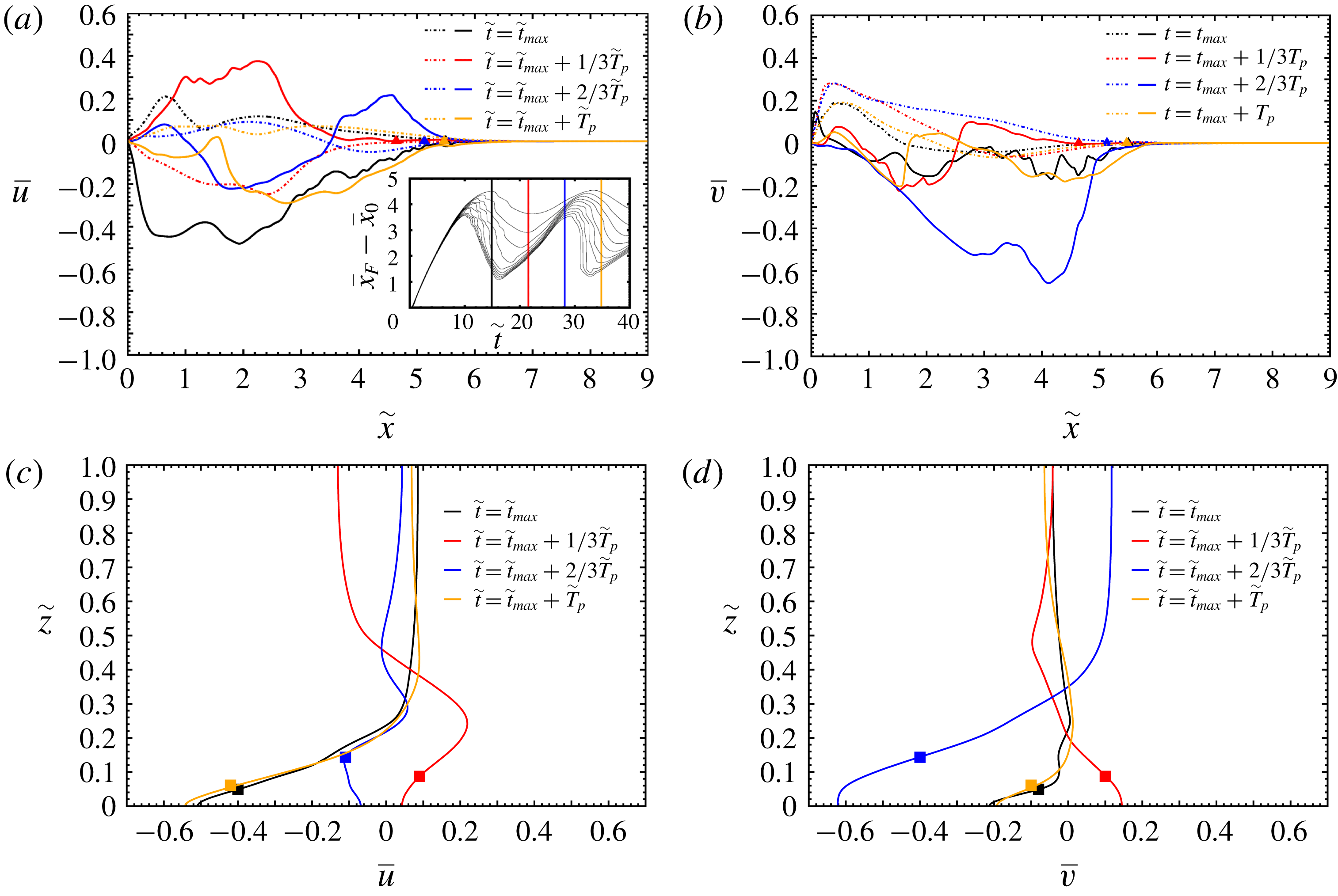
Figures 11 and 12 present span-averaged velocity profiles along some specific horizontal or vertical lines, during the first oscillation (
 $\tilde{t}_{max}\leqslant \tilde{t}\leqslant \tilde{t}_{max}+\tilde{T}_{p}$
) for case S1-C15-F and S1-C15-N, respectively. The oscillation phenomenon is noticeable since all the velocities change sign from one instant to another.
Span-averaged velocity profiles at various moments during the first oscillation (case S1-C15-F): (a)
 $\overline{u}(\tilde{x})$
at
 $\tilde{z}=0.1$
(solid) and 0.9 (dashed); (b)
 $\overline{v}(\tilde{x})$
at
 $\tilde{z}=0.1$
(solid) and 0.9 (dashed); (c)
 $\overline{u}(\tilde{x}=3,\tilde{z})$
; (d),
 $\overline{v}(\tilde{x}=3,\tilde{z})$
. The symbols indicate the location of the interface of the current, here defined as
 $\tilde{z}=\overline{h}$
(square) or
 $\tilde{x}=\overline{x}_{F}$
using
 $\unicode[STIX]{x1D6FF}=0.01$
(triangle). Here,
 $\tilde{t}_{max}=14.9$
and
 $\tilde{T}_{p}=19.51$
.
Same as figure 11 for case S1-C15-N. Here,
 $\tilde{t}_{max}=17.6$
and
 $\tilde{T}_{p}=19.76$
.

Effect of the bottom boundary condition and Schmidt number on the shape of the wedge when (quasi-)geostrophic adjustment is reached (same as figure 8 at time
 $\tilde{t}=200$
). The white solid line is the equivalent height
 $\overline{h}$
. (– ⋅ – ⋅ –, red) SW ‘steady wedge’ solution (3.9); (– ⋅ – ⋅ –, blue) SW ‘steady wedge’ solution (3.12). A movie of cases S1-C15-N and S5-C15-N (Movie 7) is available in the supplementary materials.

We display in figure 11(a) the streamwise distribution of the streamwise velocity in the current close to the bottom boundary (solid lines), and in the ambient close to the top boundary (dash-dotted lines). At
 $\tilde{t}=\tilde{t}_{max}$
, the current is propagating inward and a large part of the front region in the current
 $2\leqslant \tilde{x}\leqslant \tilde{x}_{N}$
is subject to stretching as
 $\tilde{u} <0$
and
 $\unicode[STIX]{x2202}\tilde{u} /\unicode[STIX]{x2202}\tilde{x}>0$
. At
 $\tilde{t}=\tilde{t}_{max}+\tilde{T}_{p}/3$
, the current is propagating outward and the fluid in the current
 $2.5\leqslant \tilde{x}\leqslant \tilde{x}_{N}$
is subject to compression as
 $\tilde{u} >0$
and
 $\unicode[STIX]{x2202}\tilde{u} /\unicode[STIX]{x2202}\tilde{x}<0$
. The situation is reversed at
 $\tilde{t}=\tilde{t}_{max}+2\tilde{T}_{p}/3$
as the current is mostly stretched (note that a small region close to the front is still in compression at this time). The distribution of
 $\tilde{u}$
at
 $\tilde{t}=\tilde{t}_{max}+\tilde{T}_{p}$
is roughly similar to that at
 $\tilde{t}=\tilde{t}_{max}$
and one may expect the above-mentioned observations to be similar for the next cycles. The description of the flow in the ambient is analogous to that in the current since the velocity distributions are observed to be, at first order, symmetrical.
The streamwise distribution of the anticyclonic (lateral) velocity is presented in figure 11(b). Before describing this figure, it worth recalling that the SW theoretical model predicts that
 $\tilde{v}=-2{\mathcal{C}}\tilde{x}$
(see (3.12)) as soon as the wedge is steady. Here, one can see that this trend is barely observed in the present velocity profiles, except maybe at
 $\tilde{t}=\tilde{t}_{max}+2\tilde{T}_{p}/3$
where a somewhat linear evolution of
 $\tilde{v}$
with
 $\tilde{x}$
may be seen. Beside that, the anticyclonic velocity changes sign at several places in the current and the local maximum values are an order of magnitude less than
 $\tilde{v}(\tilde{x}_{N})$
predicted by the SW theoretical model (
 ${\approx}0.15$
versus
 ${\approx}1.3$
).
The vertical distribution of the streamwise and anticyclonic velocity displayed in figures 11(c) and 11(d), respectively, clearly exhibits two regions of opposite sign. We denote by
 $\tilde{z}^{\tilde{u} =0}$
(
 $\tilde{z}^{\tilde{v}=0}$
) the vertical location where
 $\tilde{u} =0$
(
 $\tilde{v}=0$
). In general,
 $\tilde{z}^{\tilde{u} =0}$
and
 $\tilde{z}^{\tilde{v}=0}$
are not identical. In addition, they are two to four times as large as
 $\tilde{z}=\overline{h}$
. It is worth mentioning that at
 $\tilde{t}=\tilde{t}_{max}+2\tilde{T}_{p}/3$
, the streamwise velocity
 $\tilde{u}$
is zero at three locations
 $\tilde{z}^{\tilde{u} =0}\approx 1.5\overline{h}$
,
 $2\overline{h}$
and
 $3\overline{h}$
.
The same observations can be made regarding the span-averaged velocity profiles for the case S1-C15-N where no-slip boundary conditions are used at the bottom and top walls (figure 12).
In figure 13 we present the span-averaged density field
 $\overline{\unicode[STIX]{x1D70C}}$
and equivalent height
 $\overline{h}$
at time
 $\tilde{t}=200$
when (quasi-)geostrophic adjustment is reached, for various types of bottom boundary condition and Schmidt numbers. Contrary to the results of figure 8 (showing the same currents at an early time before the first arrest of the front), the shape of the currents is here a strong function of the type of bottom boundary condition and the Schmidt number. This is to be expected since at such a large time (
 ${\approx}10\tilde{T}_{p}$
) the current has reached a quasi-steady shape and can be considered, at first order, at rest, notwithstanding the oscillations and the slow drift of the current, and thus mass diffusion may play a role. Moreover, computing
 $\unicode[STIX]{x1D706}$
(see (4.2)) for the results presented in figure 13 at time
 $\tilde{t}=200$
, one finds
 $\unicode[STIX]{x1D706}=0.272$
,
 $\unicode[STIX]{x1D706}=0.298$
,
 $\unicode[STIX]{x1D706}=0.221$
and
 $\unicode[STIX]{x1D706}=0.093$
, for cases S1-C15-F, S1-C15-N, S5-C15-N and SI-C15-N, respectively. As seen in figure 8 for
 $\tilde{t}=10$
, mixing at the interface is larger for cases with no-slip boundary conditions, for the same Schmidt number. Moreover, mixing decreases as Schmidt number increases. Note that reasonable agreement is observed between the shape of the S1-C15-F current and the SW predictions (3.9) and (3.12).
4.3 Slow drift of the front (spin-up effect)
As mentioned at the end of § 4.2.1, figure 9, which presents the temporal evolution of the front displacement for various bottom boundary conditions and Schmidt numbers, shows a slow ‘drift’ of the front. This drift is observed to be significantly faster at large Schmidt number and when a no-slip condition is used at the bottom wall.
We interpret this slow drift of the front displacement as a spin-up effect, using the SW theoretical model described in § 3.3. The SW model (3.17) and (3.21) shows that the rate of the drift (or spin-up effect) increases with increasing Coriolis number, Ekman number and when using a no-slip boundary condition (via the coefficient
 $k$
; see (3.19)). Note, however, that the SW model is independent of the Schmidt number and hence is not able to capture the increase in the drift with respect to
 $Sc$
.
In order to quantify the effect of
 ${\mathcal{C}}$
,
 $Sc$
and the type of top–bottom boundary condition on the slow drift of the front, we present in table 2 the mean drift velocity
 $\text{d}\overline{x}_{F}/\text{d}\tilde{t}$
obtained in the DNS and the SW model without mixing (3.17) and with mixing (3.21). The mean drift velocity is computed from the DNS via the slope of the best-fit lines of
 $\overline{x}_{F}-\overline{x}_{0}$
in figures 2 and 9, using
 $\unicode[STIX]{x1D6FF}=0.01$
in the interval
 $100<\tilde{t}<200$
(dashed red lines). Similarly for the SW, the mean drift velocity is the slope of the blue and orange dashed lines in these figures (over the same interval).
Mean ‘drift’ velocity
 $\text{d}\overline{x}_{F}/\text{d}\tilde{t}$
of the slow expanding front (computed for
 $\tilde{t}\geqslant 100$
) corresponding to the slope of the dashed lines in figures 2 and 9. DNS refers to the fully resolved simulations (see table 1) and SW refers to the shallow-water theoretical model without mixing (3.17) and with mixing (3.21).
 $FS$
and
 $NS$
refer to free slip and no slip for DNS, and to
 $k=1/2$
and
 $3/2$
(see § 3.3 for definition) for SW, respectively.

One can clearly see in table 2 that the mean drift velocity in the DNS strongly increases when
 $Sc$
is increased. For instance,
 $\text{d}\overline{x}_{F}/\text{d}\tilde{t}$
is about nine times as large at
 $Sc=\infty$
than at
 $Sc=1$
when free-slip boundary conditions are used (more than 20 times with no-slip boundary conditions). Again, the SW model cannot capture the present observations.
Regarding boundary conditions, the mean drift velocity in the DNS increases by a factor of about 4–20 when wall friction is present at the bottom wall (the factor being a function of the Schmidt number). The SW model gives a similar trend, since
 $\text{d}\overline{x}_{F}/\text{d}\tilde{t}$
is increased by a factor of 3 from a configuration where there is free slip at the bottom wall (i.e.
 $k=1/2$
) to a configuration where there is no slip (
 $k=3/2$
). The agreement between DNS and the SW without mixing, however, is only qualitative since the specific value of the mean drift velocity predicted by the SW model is in general an order of magnitude smaller than in the DNS. However, when mixing is included in the SW model (3.21), the agreement is significantly improved. This supports the idea that the turbulent mixing in the interfacial region between the current and the ambient plays a significant role in reducing the angular velocity and hence is a key process at play during the slow drift of the front.
The influence of the Coriolis number on the drift of the front is less pronounced, as compared to the other parameters, at least for the present range
 $0.1\leqslant {\mathcal{C}}\leqslant 0.25$
. Indeed,
 $\text{d}\overline{x}_{F}/\text{d}\tilde{t}$
varies by a factor of 2–3 depending on the approach (DNS or SW). As for the DNS,
 $\text{d}\overline{x}_{F}/\text{d}\tilde{t}$
is observed to decrease when
 ${\mathcal{C}}$
is increased, and vice versa for SW. In order to verify that the present trend observed in the DNS is independent of the way
 $\text{d}\overline{x}_{F}/\text{d}\tilde{t}$
is calculated, we also computed
 $\text{d}\overline{x}_{F}/\text{d}\tilde{t}$
using
 $\tilde{\unicode[STIX]{x1D70C}}=0.01$
instead of
 $\unicode[STIX]{x1D6FF}=0.01$
. This is equivalent to calculating the slope of the best-fit line of
 $\overline{x}_{F}-\overline{x}_{0}$
in figure 15 using
 $\tilde{\unicode[STIX]{x1D70C}}=0.01$
in the interval
 $100<\tilde{t}<200$
. It turns out that such a calculation gives
 $\text{d}\overline{x}_{F}/\text{d}\tilde{t}=2\times 10^{-4}$
,
 $6\times 10^{-4}$
and
 $5\times 10^{-4}$
for
 ${\mathcal{C}}=0.1$
, 0.15 and 0.25, respectively. Using this indicator for the DNS, one may be tempted to conclude that the trend roughly follows that of the SW model. This shows that the DNS results in the first three lines of table 2 are somewhat ambiguous and do not allow us to conclude regarding the influence of the Coriolis number on the slow drift of the front. One may need to cover a larger range of
 ${\mathcal{C}}$
than that presently covered, which must be left for future work.
Spin-up
 $-\unicode[STIX]{x1D714}=-\tilde{v}/({\mathcal{C}}\tilde{x})$
as a function of
 $K_{su}^{m}t$
,
 $t$
scaled with
 $1/\unicode[STIX]{x1D6FA}$
(here
 $t={\mathcal{C}}\tilde{t}$
): (dashed line) SW theoretical model with mixing, solution of (3.21); (solid line) DNS, maximum angular velocity for case S1-C15-N.

The spin-up effect is presented in figure 14 via the time evolution of the angular velocity obtained from the SW model (3.21) and one DNS. As for the SW model (dashed line), the decay of
 $\hat{\unicode[STIX]{x1D714}}=\tilde{v}/({\mathcal{C}}\tilde{x})$
is initially quite fast, but after decay to 1 at
 $t\approx 1.3/K_{su}^{m}$
(scaled with
 $\unicode[STIX]{x1D6FA}$
), the process slows down significantly. Reduction to 25 % of the initial value takes about
 $2.8(K_{su}^{m}\unicode[STIX]{x1D6FA})^{-1}$
time or
 $0.45/K_{su}^{m}$
revolutions. In any case, the spin-up influence requires many revolutions of the system. Let us also keep in mind that
 $x_{N}\propto \tilde{\unicode[STIX]{x1D714}}^{-1/3}$
, which means that a relatively small spread of the wedge, 26 %, is expected while
 $\tilde{\unicode[STIX]{x1D714}}$
decays from 2 to 1.
For comparison, the time evolution of the maximum angular velocity obtained from the DNS is also plotted in figure 14 (case S1-C15-N, solid line). The trend between the SW theoretical model and the DNS is similar. Note that the observed oscillations of
 $\hat{\unicode[STIX]{x1D714}}$
in the DNS are due to the oscillations of the front (figure 9
b). When the latter is arrested and goes backward, the Coriolis force sharply decreases (and changes sign), as does the angular velocity. Recall also that for the DNS, we plot the maximum angular velocity which is likely to be sensitive to the various changes in the dynamics. The time scales between the SW model including mixing (3.21) and DNS are of the same order of magnitude, even though not exactly the same. Note that this is not the case for the SW model without mixing (3.17), which largely underestimates the rate of decay of
 $\hat{\unicode[STIX]{x1D714}}$
(not shown).
5 Summary and discussions
In this work we have investigated the propagation of finite-volume planar rotating gravity currents by means of fully resolved direct numerical simulations (DNS) and a shallow-water theoretical model (SW). We have considered a range of relatively small Coriolis numbers (
 $0.1\leqslant {\mathcal{C}}\leqslant 0.25$
), a large range of Schmidt numbers (
 $1\leqslant Sc<\infty$
) and two types of top–bottom boundary conditions (free-slip and no-slip). The simulations cover all the phases of propagation, including (i) the early times of spreading until the first arrest of the front and the subsequent geostrophic adjustment characterized by (ii) inertial oscillations of the front and (iii) a slow expansion of the maximum location of the front due to the so-called spin-up effect.
(1) Early times of propagation until the first arrest of the front. DNS and SW are in reasonable agreement. Both approaches confirm that the location of the first arrest of the front is a decreasing function of
 ${\mathcal{C}}$
. DNS shows that this location is roughly independent of
 $Sc$
and the type of top–bottom boundary conditions (within 15 %). Note that the SW model generally slightly overestimates the front speed (by 15–20 %) and underestimates the time and location of the first arrest. This may be explained by the fact that since the SW model neglects viscous effects, the local velocity is generally larger, as is the Coriolis force. As a consequence, the front stops earlier at a smaller location.
The location of the first arrest of the front in the DNS has been compared to the SW asymptotic solution (3.12) for the length of the steady-state wedge, in the limit of small Coriolis numbers. In particular, (3.12) predicts that the length of the wedge is
 $\propto {\mathcal{C}}^{-2/3}$
. The DNS results, when compared to available data for rotating cylindrical currents, seem to corroborate this scaling law. Note however, that more simulations (or experiments) are needed to allow for a definite conclusion regarding the relevance of (3.12).
(2) Geostrophic adjustment and inertial oscillations. When the front has reached a maximum location, it subsequently oscillates around a characteristic position at a constant pulse frequency. The pulse frequency found in the DNS is in agreement (within 9 %) with that of inertial waves, i.e.
 $\overline{\unicode[STIX]{x1D714}}_{p}=2{\mathcal{C}}$
. In addition, the DNS results show that
 $\overline{\unicode[STIX]{x1D714}}_{p}$
is independent of
 $Sc$
and the type of top–bottom boundary conditions.
Another noticeable feature obtained from the DNS results during the inertial oscillations at
 $0.1\leqslant {\mathcal{C}}\leqslant 0.25$
is that the front of the current is much thicker than in non-rotating configurations (
 ${\mathcal{C}}=0$
). We explain this by the fact that the rotating front is subject to (i) enhanced mixing stemming from Kelvin–Helmholtz instability generated by the shear in the spanwise direction and (ii) local stretching in the front region which smoothes the local density gradient.
(3) Slow ‘drift’ of the front. When turbulent mixing is included in the SW spin-up model, DNS and SW are in reasonable agreement. DNS shows that the mean ‘drift’ velocity of the expanding front strongly increases with increasing
 $Sc$
and with the presence of wall friction (up to an order of magnitude). The SW model only captures the trend with respect to wall friction since it is independent of the Schmidt number. In any case, this supports the idea that friction, due to turbulent mixing in the interfacial region, is (at least) one process responsible for the slow drift of the front.
Overall, it must be emphasized that the present work has raised more questions concerning the ‘drift’ stage than it has answered. In particular, it is the first time that, to our best knowledge, such a significant effect of the Schmidt number has been observed for the slow drift of the front of rotating gravity currents. The physical processes responsible for such a behaviour are, to the authors, still an open question which is left for future work. On the other hand, the results and insights concerning the earlier stages of the motion are, in our opinion, reliable and can be used with confidence for applications and further research. The laboratory-test confirmation is still needed, and we hope that this paper will provide the guidelines and motivation for such experimental studies.
Acknowledgements
Some of the computation time was provided by the Scientific Groupment CALMIP (projects P1525), the support of which is greatly appreciated. T.B. thanks Toulouse INP, Université de Toulouse and IMFT for financial support for some visiting exchanges of T.B., M.I.C. and M.U., respectively. The authors also thank the anonymous reviewers for their useful comments, in particular one of the referees for having pointed out the importance of mixing and entrainment on the slow expansion of the front at late times.
Supplementary movies
Supplementary movies are available at https://doi.org/10.1017/jfm.2019.152.
Appendix. On the computation of the front displacement
Time evolution of the front displacement
 $\overline{x}_{F}-\overline{x}_{0}$
for
 ${\mathcal{C}}=0.1$
(a), 0.15 (b), 0.25 (c), where
 $\overline{x}_{F}$
is defined as the maximum location where the span-averaged density field at the bottom wall is
 $\overline{\unicode[STIX]{x1D70C}}=0.01$
, 0.1, 0.2, 0.3, 0.4 and 0.5, respectively.

As mentioned in § 4.1, a method for measuring the displacement of the front is the tracking of the density at the bottom of the channel. After the computation of the span-averaged density function
 $\overline{\unicode[STIX]{x1D70C}}$
, we track different values of
 $\overline{\unicode[STIX]{x1D70C}}$
at
 $\tilde{z}=0$
. The time evolution of the front displacement
 $\overline{x}_{F}-\overline{x}_{0}$
for
 ${\mathcal{C}}=0.1$
(a), 0.15 (b), 0.25 (c), using this method is presented in figure 15 and may be compared to figure 2. Even if the precise position or expansion of the front region is not strictly identical between the two methods, the trend is similar. In particular, figure 15 confirms that the interface separating the current and the ambient does not remain sharp in rotating gravity currents and that the method used in this work to locate the front region is pertinent.



