1 Introduction
As reviewed by Stone, Stroock & Ajdari (Reference Stone, Stroock and Ajdari2004) and Darhuber & Troian (Reference Darhuber and Troian2005), surface-tension modulation is often utilised for microfluidic devices used in such applications as DNA microarrays, drug screening and optical display technologies. As a force per unit length, surface tension becomes dominant over body forces (e.g. inertia, gravity) and surface forces (pressure and viscous stresses) at small length scales, allowing liquid to be controlled efficiently. Possible ways to utilise surface tension are in causing surface-tension gradients or controlling wettability, which is a surface-tension effect on a solid surface. In particular, electrowetting, which involves using an electric field to change the wettability, is expected to be a very useful technology because of the ease of electronic control and its low power consumption. The study of electrowetting began with Lippmann (1875) (English translation available in appendix of Mugele & Baret (Reference Mugele and Baret2005)), followed by various evolutions (see reviews by Quilliet & Berge (Reference Quilliet and Berge2001), Mugele & Baret (Reference Mugele and Baret2005), Fair (Reference Fair2007), Mugele (Reference Mugele2009), Mugele, Duits & van den Ende (Reference Mugele, Duits and van den Ende2010), Chen & Bonaccurso (Reference Chen and Bonaccurso2014)).
Being able to predict the shape and speed of droplets is very important in the design and operation of microfluidic devices. Ren et al. (Reference Ren, Fair, Pollack and Shaughnessy2002), Cho, Moon & Kim (Reference Cho, Moon and Kim2003), Song et al. (Reference Song, Evans, Lin, Hsu and Fair2009) and Suzuki et al. (Reference Suzuki, Homma, Murayama, Fukuda, Takanobu and Miura2010) have studied droplet manipulation by electrowetting on dielectric (EWOD) both experimentally and theoretically. Mugele et al. (Reference Mugele, Klingner, Buehrle, Steinhauser and Herminghaus2005), Mugele & Buehrle (Reference Mugele and Buehrle2007), Oh, Ko & Kang (Reference Oh, Ko and Kang2008) and Oh, Ko & Kang (Reference Oh, Ko and Kang2010) have studied the shape of droplets in an applied electric field. Ko, Lee & Kang (Reference Ko, Lee and Kang2008) have visualised droplet-interior flows generated by electrowetting. Berthier et al. (Reference Berthier, Clementz, Raccurt, Jary, Claustre, Peponnet and Fouillet2006) and Lienemann, Greiner & Korvink (Reference Lienemann, Greiner and Korvink2006) have used numerical simulations to study equilibrium drop shape by means of a surface evolver (Brakke Reference Brakke1992), which is based on the principle of minimising free energy. However, the equilibrium approach cannot represent the dynamics of droplet movement and so cannot be used to estimate the time scales of movement or deformation. Blake, Clarke & Stattersfield (Reference Blake, Clarke and Stattersfield2000) analysed film coating speed with electrowetting assisted by molecular kinetic theory, and McHale, Brown & Sampara (Reference McHale, Brown and Sampara2013) analysed voltage-induced spreading of a droplet using a dynamic contact-angle model considering viscous dissipation similar to de Gennes (Reference de Gennes1985). Zeng (Reference Zeng2006) invoked the electrohydrodynamic force to simulate droplet splitting, but the detailed fluid dynamics was unclear and the results were not discussed fully. Fontelos et al. (Reference Fontelos, Grün, Kindelán and Klingbeil2012) performed a three-dimensional numerical simulation of electrowetting droplet movement considering electrohydrodynamics fully, however, validation of the computation was not shown.
To predict droplet dynamics precisely, a computational fluid dynamics approach may be useful. Walker & Shapiro (Reference Walker and Shapiro2006) used a level-set method, Lu et al. (Reference Lu, Glasner, Bertozzi and Kim2007) used a diffuse-interface model and Walker, Shapiro & Nochetto (Reference Walker, Shapiro and Nochetto2009) used a finite-element method, all subject to the Hele-Shaw approximation so that the computations were two-dimensional. Mondal et al. (Reference Mondal, Ghosh, Bandopadhyay, DasGupta and Chakraborty2013) used a diffuse-interface model and Li, He & Zhang (Reference Li, He and Zhang2013) used a form of the front-tracking method, both restricted to two-dimensional systems. In the three-dimensional case, Takada et al. (Reference Takada, Matsumoto, Matsumoto and Ichikawa2008) performed diffuse-interface simulations, but assumed changes in wettability in a non-electrical context. Under the Hele-Shaw approximation, the two-dimensional velocity field is determined solely by the pressure gradient and so the effect of wettability has to be embedded through a pressure boundary condition. Lu et al. (Reference Lu, Glasner, Bertozzi and Kim2007) considered wettability in the context of single-parameter EWOD, but their simulation could not reproduce the time scales of droplet movement or splitting as measured in their experiments. Although they tried to adjust the parameters, their simulations produced either splitting that was too fast or no splitting at all. In the present state, fully three-dimensional simulations are needed to represent wettability precisely.
Until now, there has been no fully three-dimensional simulation of a detailed electrowetting scenario which considers the dynamic contact angle fully. Our group (Yamamoto et al. Reference Yamamoto, Ito, Wakimoto and Katoh2013, Reference Yamamoto, Tokieda, Wakimoto, Ito and Katoh2014) has developed a simulation code that uses front tracking (Unverdi & Tryggvason Reference Unverdi and Tryggvason1992) to represent dynamic wetting subject to the generalised Navier boundary condition (Qian, Wang & Sheng Reference Qian, Wang and Sheng2003), and has extended it to a fully three-dimensional code (Yamamoto et al. Reference Yamamoto, Higashida, Tanaka, Wakimoto, Ito and Katoh2016). In the present study, we perform the fully three-dimensional simulations of droplet movement in a narrow gap actuated by EWOD by using front tracking and subject to the generalised Navier boundary condition and the Young–Lippmann equation. In addition, we propose a simple theoretical model of droplet movement, and we consider droplet dynamics by means of numerical experiments and theoretical analyses.
The remainder of this paper proceeds as follows. In § 2, we describe the target system of this study. In § 3, we describe the theoretical modelling and its evaluation by comparison with experimental data. In § 4, we describe the method of numerical simulation and compare the results from simulation and experiment. In § 5, we present the results of numerical experiments with various parameter values, and discuss the motion using a theoretical model. Finally, in § 6, we summarise our results.
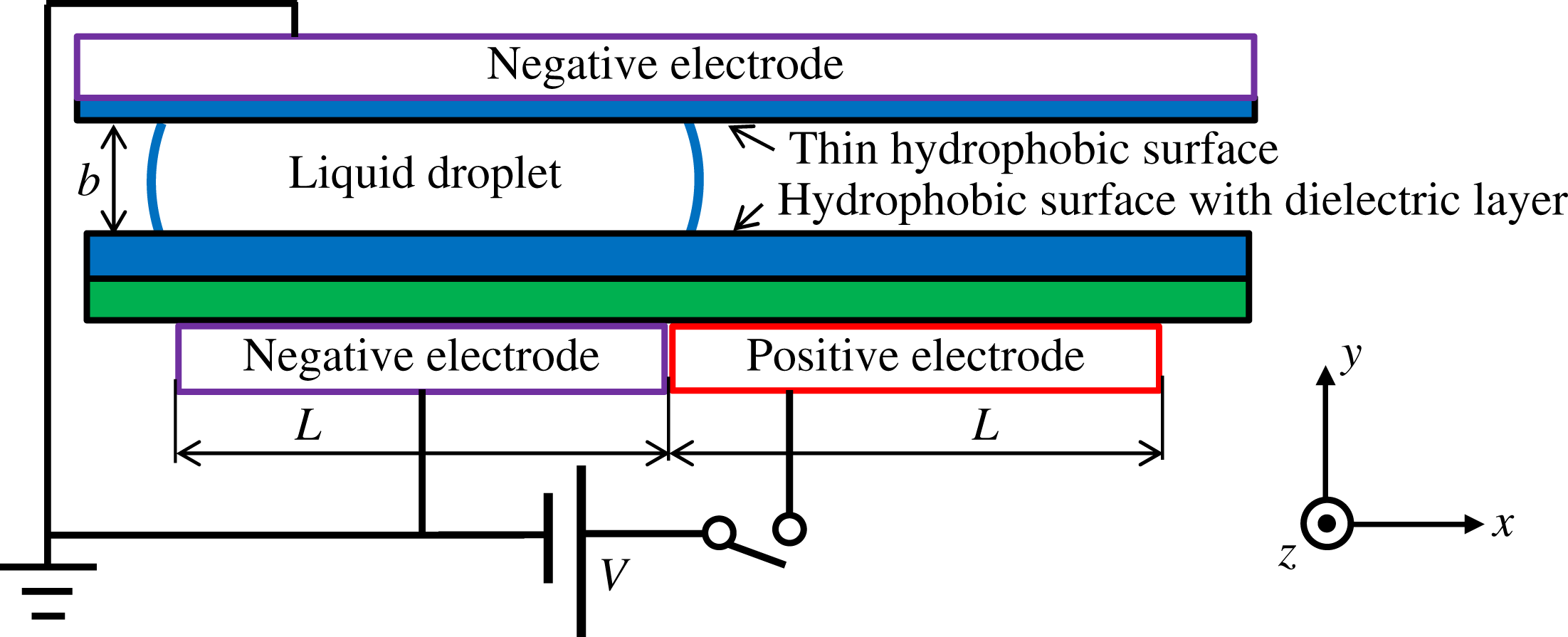
Configuration of target system.

2 Target system
As the target system in this study, as shown in figure 1, we chose a narrow gap between two parallel flat plates in which a droplet moves by EWOD, similar to the experiments of Cho et al. (Reference Cho, Moon and Kim2003) and Lu et al. (Reference Lu, Glasner, Bertozzi and Kim2007). In the present study, we treat only droplet movement as the simplest case in such an EWOD system; we leave splitting and merging for future work. The bottom plate contains rectangular electrodes below a hydrophobic surface with a dielectric layer. The top plate contains a large negative electrode set on a very thin dielectric and hydrophobic surface. Because of the low dielectric constant of the top plate, we consider the liquid droplet between the plates to be grounded at the top plate. Hence, we consider the supplied voltage to be applied directly to the positive electrode at the bottom. As shown in figure 1, the
 $x$
direction is parallel and in line with the bottom electrodes, the
 $y$
direction is normal to the plate surfaces and the
 $z$
direction is the spanwise one. The dimensions of each electrode on the bottom plate are
 $x$
-direction length
 $L$
and
 $z$
-direction width
 $W$
. The
 $y$
-direction gap between the plates is
 $b$
, which is much smaller than the droplet size in the
 $x$
–
 $z$
plane, so the geometry approximates that of a Hele-Shaw cell. The initial radius of the droplet in the gap is
 $R$
, so the volume of the droplet can be calculated as
 $\unicode[STIX]{x03C0}R^{2}b$
. The static contact angle over the entire plate surface with no applied voltage is
 $\unicode[STIX]{x1D703}_{s0}$
, the capacitance per unit area of the bottom plate is
 $c$
and the supplied voltage is
 $V$
. Values of
 $V$
are considered in the range in which the Young–Lippmann equation (Mugele & Baret Reference Mugele and Baret2005), namely
 $$\begin{eqnarray}\cos \unicode[STIX]{x1D703}_{s}=\cos \unicode[STIX]{x1D703}_{s0}+\frac{cV^{2}}{2\unicode[STIX]{x1D70E}},\end{eqnarray}$$
is valid, where
 $\unicode[STIX]{x1D703}_{s}$
is the static contact angle at the supplied voltage
 $V$
and
 $\unicode[STIX]{x1D70E}$
is the surface tension of the liquid.
3 Dynamics of droplet motion
In this section, we derive a simple theoretical model for the motion of a droplet in a narrow gap driven by EWOD.
3.1 Theoretical modelling
The droplet is driven by surface tension, which acts in the direction of parallel to the plane prescribed by the instantaneous contact angle and perpendicular to the contact line. Here, we consider the change in contact angle due to dynamic wetting and EWOD as stated in (2.1). The dynamic contact angle
 $\unicode[STIX]{x1D703}_{d}$
can be estimated by using the Hoffmann–Voinov–Tanner law (Kistler Reference Kistler and Berg1993) as
 $$\begin{eqnarray}\unicode[STIX]{x1D703}_{d}=({\unicode[STIX]{x1D703}_{s}}^{3}+k\mathit{Ca})^{1/3},\end{eqnarray}$$
where
 $k$
is an empirical constant that depends on the experimental conditions. The term
 $\mathit{Ca}$
is the capillary number defined as
 $\mathit{Ca}=\unicode[STIX]{x1D707}_{l}U_{cl}/\unicode[STIX]{x1D70E}$
, where
 $\unicode[STIX]{x1D707}_{l}$
is the dynamic viscosity of the liquid and
 $U_{cl}$
is the speed of the contact line. We considered the generality of analysis without the assistance of numerically simulated data, so we introduced the well-used empirical relation to describe the dynamic contact angle different from the numerical model used in our simulation described later. In this modelling, the effect of unknown information such as measurement scale is put into one fitting parameter
 $k$
. In this study, we assume
 $\mathit{Ca}\sim O(10^{-3})$
, so the approximation of
 $k\mathit{Ca}\ll {\unicode[STIX]{x1D703}_{s}}^{3}$
can be used. We take cosine of equation (3.1) and perform Taylor expansion with
 $k\mathit{Ca}\ll {\unicode[STIX]{x1D703}_{s}}^{3}$
, then we have
 $$\begin{eqnarray}\cos \unicode[STIX]{x1D703}_{d}=\cos \unicode[STIX]{x1D703}_{s}-\frac{k\sin \unicode[STIX]{x1D703}_{s}}{3{\unicode[STIX]{x1D703}_{s}}^{2}}\mathit{Ca}.\end{eqnarray}$$
We substitute a front and a rear contact angle into equation (3.2) while reversing the sign of the second term on the right-hand side if required because of the sign of
 $U_{cl}$
:
 $$\begin{eqnarray}\displaystyle & \displaystyle \cos \unicode[STIX]{x1D703}_{dA}=\cos \unicode[STIX]{x1D703}_{sA}-\frac{k\sin \unicode[STIX]{x1D703}_{sA}}{3\unicode[STIX]{x1D703}_{sA}^{2}}\mathit{Ca}, & \displaystyle\end{eqnarray}$$
 $$\begin{eqnarray}\displaystyle & \displaystyle \cos \unicode[STIX]{x1D703}_{dR}=\cos \unicode[STIX]{x1D703}_{sR}+\frac{k\sin \unicode[STIX]{x1D703}_{sR}}{3\unicode[STIX]{x1D703}_{sR}^{2}}\mathit{Ca}, & \displaystyle\end{eqnarray}$$
where
 $\unicode[STIX]{x1D703}_{dA}$
and
 $\unicode[STIX]{x1D703}_{dR}$
are the front (advancing) and rear (receding) dynamic contact angles of the drop, respectively, and
 $\unicode[STIX]{x1D703}_{sA}$
and
 $\unicode[STIX]{x1D703}_{sR}$
are the advancing and receding static contact angles, respectively.
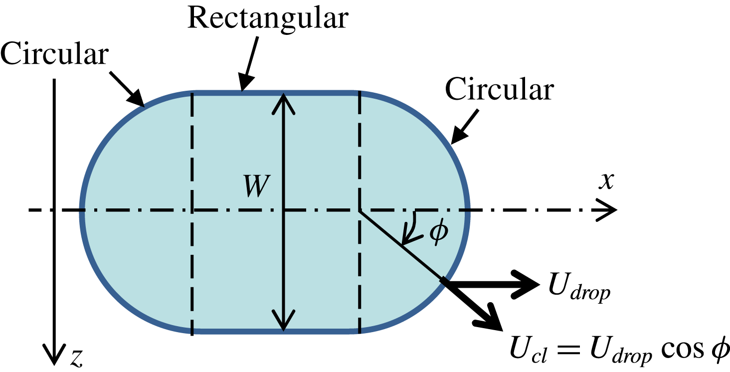
Although real droplet geometry is varied as shown in figure 5, we approximate it by simple shape as shown in figure 2 in our theoretical model. Here, for the purpose of simplicity, we assume a racetrack shape composed of two half-circles and two straight lines. From experimental observations (Lu et al.
Reference Lu, Glasner, Bertozzi and Kim2007) and numerical results shown later in § 4, the droplet shrinks quickly widthways (within 2 s) after the voltage is imposed on the electrodes and then remains as the electrode width
 $W$
as shown in figure 2. Note that the wetted surface area in the figure should be the same as that of the initial circular droplet (
 $\unicode[STIX]{x03C0}R^{2}$
) because of volume conservation in the channel. The length of the straight sections can be determined simply from this fact.
Droplet shape assumed in the present theoretical model.

The surface tension acts on the contact line on both the upper and lower walls of the channel, as shown in figure 1. As stated in § 2, the EWOD effect changes the static contact angle appearing on the lower wall at the positive electrode. In particular, the advancing contact angle
 $\unicode[STIX]{x1D703}_{sA}$
in (3.3) on the lower wall should be rewritten using (2.1). Taking both EWOD and dynamic effects into consideration, the surface-tension force acting on the contact line shown in figure 2 can now be estimated. When the droplet moves while keeping the same geometrical shape as shown in figure 2, the contact-line speed
 $U_{cl}$
at each position on the semi-circular parts may be related simply to the droplet speed
 $U_{drop}$
as
 $$\begin{eqnarray}U_{cl}=U_{drop}\cos \unicode[STIX]{x1D719},\end{eqnarray}$$
where
 $\unicode[STIX]{x1D719}$
indicates the angle along the semi-circular parts of the contact line as shown in figure 2. The surface-tension forces acting on contact lines can be obtained by integration of infinitesimal force acting on a infinitesimal arc
 $(W/2)\,\text{d}\unicode[STIX]{x1D719}$
at the position
 $\unicode[STIX]{x1D719}$
for both top and bottom walls, and its
 $x$
–component is obtained by multiplying by
 $\cos \unicode[STIX]{x1D719}$
. Using the above (2.1), (3.3), (3.4) and (3.5), the surface-tension forces on the front and rear semi-circles can be calculated from the following integrals as
(front semi-circle)
 $$\begin{eqnarray}F_{sf}=\frac{\unicode[STIX]{x1D70E}W}{2}\int _{-\unicode[STIX]{x03C0}/2}^{\unicode[STIX]{x03C0}/2}\left[2\left(\cos \unicode[STIX]{x1D703}_{sA}-\frac{k\sin \unicode[STIX]{x1D703}_{sA}}{3\unicode[STIX]{x1D703}_{sA}^{2}}\mathit{Ca}_{drop}\cos \unicode[STIX]{x1D719}\right)+\frac{cV^{2}}{2\unicode[STIX]{x1D70E}}\right]\cos \unicode[STIX]{x1D719}\,\text{d}\unicode[STIX]{x1D719}\end{eqnarray}$$
(rear semi-circle)
 $$\begin{eqnarray}F_{sr}=\frac{\unicode[STIX]{x1D70E}W}{2}\int _{-\unicode[STIX]{x03C0}/2}^{\unicode[STIX]{x03C0}/2}2\left(\cos \unicode[STIX]{x1D703}_{sR}+\frac{k\sin \unicode[STIX]{x1D703}_{sR}}{3\unicode[STIX]{x1D703}_{sR}^{2}}\mathit{Ca}_{drop}\cos \unicode[STIX]{x1D719}\right)\cos \unicode[STIX]{x1D719}\,\text{d}\unicode[STIX]{x1D719},\end{eqnarray}$$
where
 $\mathit{Ca}_{drop}$
is the non-dimensional drop speed (
 $\unicode[STIX]{x1D707}_{l}U_{drop}/\unicode[STIX]{x1D70E}$
). We note that the advancing (receding) dynamic contact angle should be associated with the front (rear) semi-circle because the contact line always moves so as to wet (dewet) the surface (Katoh et al.
Reference Katoh, Azuma, Higashine and Miyamoto2006). In (3.6) and (3.7), the integration is taken over the semi-circular parts of the contact line. The surface tension on the lateral straight lines acts normal to the droplet velocity and does not contribute to the dynamics. The sum of (3.6) and (3.7) gives the resultant of surface-tension force as
 $$\begin{eqnarray}\displaystyle F_{s} & = & \displaystyle F_{sf}+F_{sr}\nonumber\\ \displaystyle & = & \displaystyle \unicode[STIX]{x1D70E}W\left[\frac{cV^{2}}{2\unicode[STIX]{x1D70E}}+2\left(\cos \unicode[STIX]{x1D703}_{sA}-\cos \unicode[STIX]{x1D703}_{sR}\right)-\frac{\unicode[STIX]{x03C0}k}{6}\left(\frac{\sin \unicode[STIX]{x1D703}_{sA}}{\unicode[STIX]{x1D703}_{sA}^{2}}+\frac{\sin \unicode[STIX]{x1D703}_{sR}}{\unicode[STIX]{x1D703}_{sR}^{2}}\right)\mathit{Ca}_{drop}\right].\end{eqnarray}$$
The terms in the bracket refer to the electrowetting effect, resistance due to contact-angle hysteresis for top/bottom walls and dynamic contact-angle effect at front/rear of top/bottom walls.
Next, we consider the forces resisting the droplet motion, namely the inertial force and the viscous drag on the wall. The inertial force can be estimated by considering the moving mass per unit time and velocity as
 $$\begin{eqnarray}F_{inert}\sim \unicode[STIX]{x1D70C}_{l}WbU_{drop}^{2},\end{eqnarray}$$
where
 $\unicode[STIX]{x1D70C}_{l}$
is the liquid density. To estimate the viscous drag, we use the time scale for the development of a viscous boundary layer as given by Stokes’ first problem (Schlichting Reference Schlichting1975). The time scale
 $t_{b}$
on which the boundary layer reaches the channel centre height
 $b/2$
can be evaluated as
 $$\begin{eqnarray}4\sqrt{\frac{\unicode[STIX]{x1D707}_{l}t_{b}}{\unicode[STIX]{x1D70C}_{l}}}=\frac{b}{2}.\end{eqnarray}$$
If
 $t_{b}$
is much smaller than the time scale
 $b/U_{drop}$
of the droplet motion, namely
 $$\begin{eqnarray}\frac{t_{b}U_{drop}}{b}\ll 1,\end{eqnarray}$$
we can safely assume that the velocity distribution in the droplet develops as a two-dimensional laminar channel flow, namely
 $$\begin{eqnarray}u(y)=\frac{6U_{drop}}{b^{2}}\left(by-y^{2}\right).\end{eqnarray}$$
Using a Reynolds number based on the gap width, namely
 $Re=\unicode[STIX]{x1D70C}_{l}bU_{drop}/\unicode[STIX]{x1D707}_{l}$
, the time scale condition (3.11) is rewritten as
 $$\begin{eqnarray}\frac{t_{b}U_{drop}}{b}=\frac{\mathit{Re}}{64}\ll 1,\end{eqnarray}$$
and this condition is satisfied in general Hele-Shaw systems for microfluidics (
 $\mathit{Re}\lesssim O(1)$
). The viscous drag can then be obtained over the whole wetted surface area (
 $2\unicode[STIX]{x03C0}R^{2}$
) as
 $$\begin{eqnarray}F_{v}=\frac{12\unicode[STIX]{x03C0}R^{2}\unicode[STIX]{x1D707}_{l}U_{drop}}{b}=\frac{12\unicode[STIX]{x03C0}R^{2}\unicode[STIX]{x1D70E}}{b}\mathit{Ca}_{drop}.\end{eqnarray}$$
When the inertial force is much smaller than the viscous force, namely
 $$\begin{eqnarray}\frac{F_{inert}}{F_{v}}\sim \frac{\unicode[STIX]{x1D70C}_{l}bU_{drop}}{\unicode[STIX]{x1D707}_{l}}\frac{b}{W}\sim Re\frac{b}{W}\ll 1,\end{eqnarray}$$
(this condition is also satisfied in general Hele-Shaw systems for microfluidics (
 $\mathit{Re}\lesssim O(1)$
and
 $b\ll W$
)), we can consider a simple force balance between surface tension and viscous drag as a good approximation for the steady state. From equations (3.8) and (3.14), the non-dimensional droplet speed in the channel can be obtained as
 $$\begin{eqnarray}\mathit{Ca}_{drop}=\frac{\displaystyle \frac{cV^{2}}{2\unicode[STIX]{x1D70E}}+2\left(\cos \unicode[STIX]{x1D703}_{sA}-\cos \unicode[STIX]{x1D703}_{sR}\right)}{\displaystyle \frac{12\unicode[STIX]{x03C0}R^{2}}{bW}+\frac{\unicode[STIX]{x03C0}k}{6}\left(\frac{\sin \unicode[STIX]{x1D703}_{sA}}{\unicode[STIX]{x1D703}_{sA}^{2}}+\frac{\sin \unicode[STIX]{x1D703}_{sR}}{\unicode[STIX]{x1D703}_{sR}^{2}}\right)}.\end{eqnarray}$$
The first term in the numerator represents the electrowetting effect and the second term represents the contact-angle hysteresis. The first term in the denominator is a non-dimensional geometrical parameter representing the effect of both driving and resistance force and the second term represents the dynamic wetting. Equation (3.16) shows that the droplet speed is determined by these four effects.
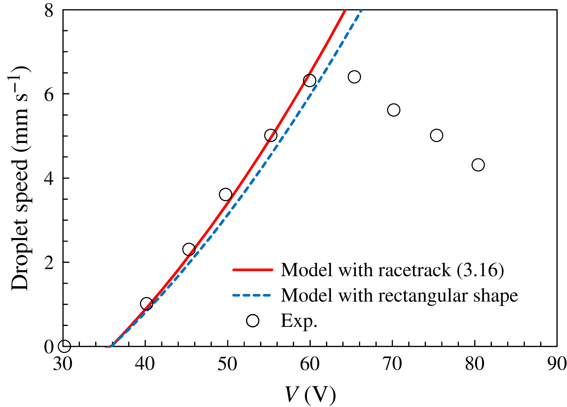
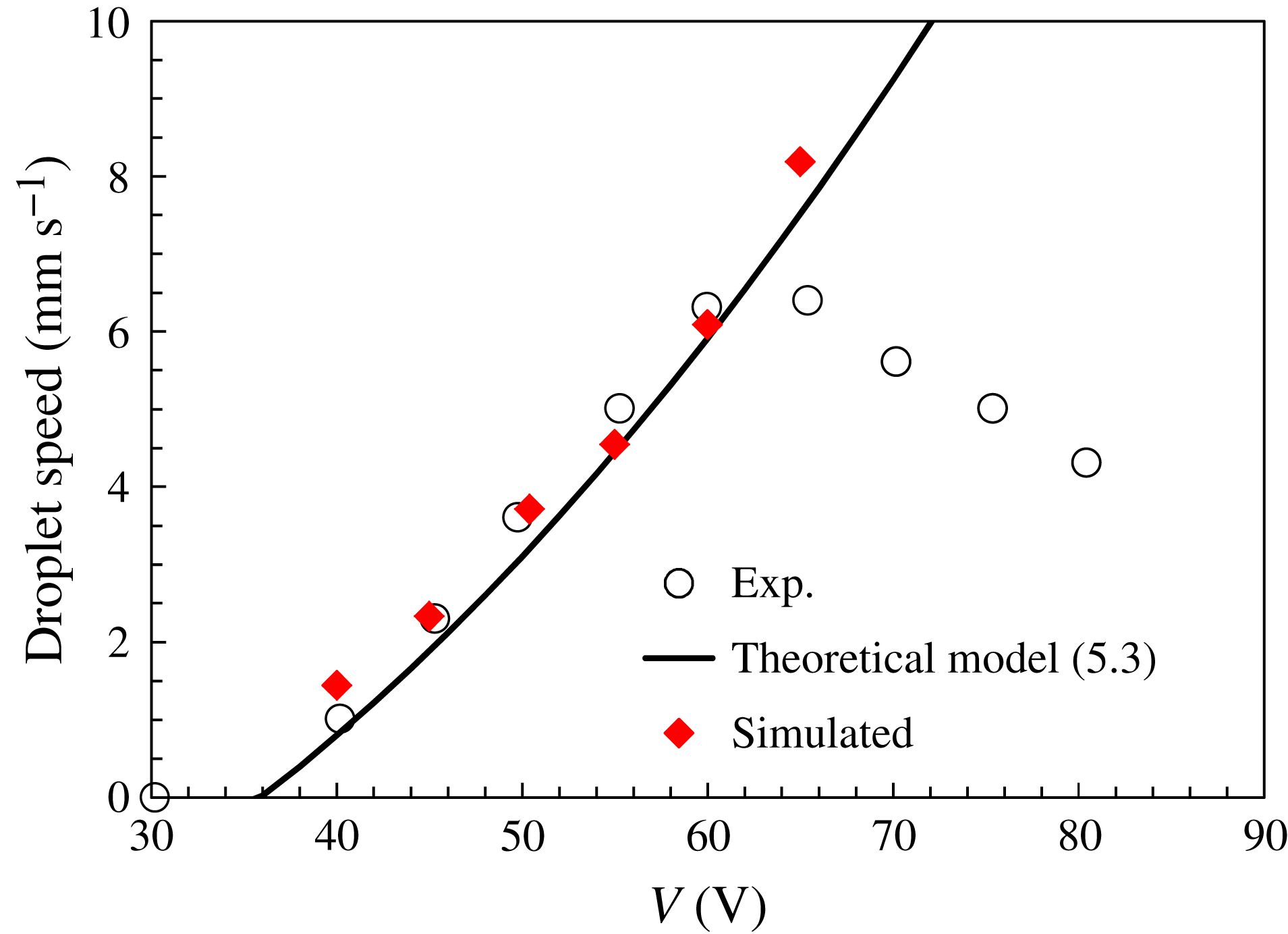
Droplet speed as estimated by the present theoretical model. Experimental data are from Lu et al. (Reference Lu, Glasner, Bertozzi and Kim2007).

3.2 Model evaluation using experimental results
Here, we evaluate the present theoretical model by using the experimental results of Lu et al. (Reference Lu, Glasner, Bertozzi and Kim2007). In their paper, the measurement condition of the equilibrium contact angle (
 $100^{\circ }$
) is unclear, so instead we estimate the equilibrium contact angle
 $\unicode[STIX]{x1D703}_{0}$
for our model from their data on the advancing and receding contact angles. From figure 6 in Lu et al. (Reference Lu, Glasner, Bertozzi and Kim2007), the steady dynamic advancing angle of the top plate (without the electrowetting effect) is
 $111^{\circ }$
and the steady dynamic receding angle (averaged from the top and bottom plates) is
 $96^{\circ }$
. Hence, we set
 $\unicode[STIX]{x1D703}_{0}$
as the average of those two values, namely
 $103.5^{\circ }$
. We also assume that the static advancing and receding contact angles are shifted equally by
 $\unicode[STIX]{x1D6FC}$
from
 $\unicode[STIX]{x1D703}_{0}$
:
 $$\begin{eqnarray}\unicode[STIX]{x1D703}_{sA}=\unicode[STIX]{x1D703}_{0}+\unicode[STIX]{x1D6FC},\quad \unicode[STIX]{x1D703}_{sR}=\unicode[STIX]{x1D703}_{0}-\unicode[STIX]{x1D6FC}.\end{eqnarray}$$
From figure 4 in Lu et al. (Reference Lu, Glasner, Bertozzi and Kim2007), the minimum voltage at which the droplet moves can be estimated as
 $V_{0}=36~\text{V}$
, at which we have
 $\mathit{Ca}_{drop}=0$
. Hence, we obtain the following from equation (3.16):
 $$\begin{eqnarray}0=\frac{cV_{0}^{2}}{2\unicode[STIX]{x1D70E}}+2\left[\cos (\unicode[STIX]{x1D703}_{0}+\unicode[STIX]{x1D6FC})-\cos (\unicode[STIX]{x1D703}_{0}-\unicode[STIX]{x1D6FC})\right].\end{eqnarray}$$
By solving (3.18), we obtain
 $\unicode[STIX]{x1D6FC}=5.1^{\circ }$
, then (3.17a,b
) yields
 $\unicode[STIX]{x1D703}_{sA}=108.6^{\circ }$
and
 $\unicode[STIX]{x1D703}_{sR}=98.4^{\circ }$
. Furthermore, from figure 11 in Lu et al. (Reference Lu, Glasner, Bertozzi and Kim2007), we can estimate the capillary number
 $\mathit{Ca}$
at which the dynamic contact angles achieve steady values as being
 $\mathit{Ca}=1.23\times 10^{-3}$
. Hence, we can determine the coefficient
 $k$
as
 $k=335$
by averaging values obtained from (3.3) and (3.4).
From the above values and the experimental conditions of Lu et al. (Reference Lu, Glasner, Bertozzi and Kim2007) (
 $c=3.6\times 10^{-5}~\text{F m}^{-2}$
,
 $\unicode[STIX]{x1D70E}=0.067~\text{N m}^{-1}$
,
 $R=5.5\times 10^{-3}~\text{m}$
,
 $b=5.3\times 10^{-4}~\text{m}$
,
 $W=1\times 10^{-2}~\text{m}$
,
 $\unicode[STIX]{x1D70C}_{l}=1.28\times 10^{3}~\text{kg m}^{-3}$
and
 $\unicode[STIX]{x1D707}_{l}=0.02~\text{Pa s}$
), we obtain the relationship shown in figure 3 between average droplet speed and applied voltage. The conditions imposed by (3.11) and (3.15) are satisfied because
 $t_{b}U_{drop}/b=O(10^{-2})$
and
 $F_{inert}/F_{v}\sim O(10^{-3})$
with
 $U_{drop}\sim 1\times 10^{-2}~\text{m}~\text{s}^{-1}$
. Up to 60 V, the present theoretical model (with racetrack shape assumption) can reproduce the experimentally measured relation very well. Above 60 V, Young–Lippmann equation (2.1) was not realised as shown in figure 2 in Lu et al. (Reference Lu, Glasner, Bertozzi and Kim2007). Increasing of the cosine of the contact angle with voltage saturates around 60 V, and it decreases above 70 V. Such contact angle saturation may be due to the dielectric break down, which has been reported by many researchers, e.g. Vallet, Berge & Vovelle (Reference Vallet, Berge and Vovelle1996), Blake et al. (Reference Blake, Clarke and Stattersfield2000). As a natural result of the contact angle increasing above 70 V, the droplet speed decreases in the experimental observation. The behaviour with the saturation voltage is outside of the scope of our interest. We only discuss the results below the saturation voltage 60 V.
In the theoretical droplet velocity described by (3.16), some experimental parameters, i.e.
 $\unicode[STIX]{x1D703}_{0}$
,
 $\unicode[STIX]{x1D6FC}$
and
 $k$
in (3.18) and (3.1) were assumed by referring the results shown in Lu et al. (Reference Lu, Glasner, Bertozzi and Kim2007). To examine the effect of parameter estimation error,
 $\unicode[STIX]{x1D703}_{0}$
was varied with
 $\pm 2^{\circ }$
. For each
 $\unicode[STIX]{x1D703}_{0}$
,
 $\unicode[STIX]{x1D6FC}$
and
 $k$
are estimated by (3.18) and (3.1), respectively. With a
 $2^{\circ }$
estimation error of
 $\unicode[STIX]{x1D703}_{0}$
, the fitted
 $k$
is varied by approximately 10 %, however, the theoretically estimated droplet speed is not so affected (below 5 % for maximum speed at 60 V). On the other hand, to examine the effect of the droplet shape assumption, as shown in figure 2, we also considered a rectangular droplet with a width of
 $W$
as an extreme example. For the rectangular droplet case, the effect of viscous drag is not changed from the racetrack case because of the constant wetted area, however, the integral of the contact-angle’s dynamic effect term in (3.6) and (3.7) depends on the contact-line shape. Then, as a result,
 $\unicode[STIX]{x03C0}$
in the second term in the denominator of (3.16) for the racetrack case is replaced by 4 for the rectangular case. In figure 3, the theoretical curve with the rectangular shape assumption is also shown. The effect of the shape assumption is not so large, the difference is approximately 8 % for a maximum speed of 60 V in the present sample cases. The present theoretical model can express the characteristic well. Later, we discuss the present model in the context of numerically simulated data with various values of the shape parameters.
4 Numerical simulations
4.1 Front-tracking method
We use the numerical procedure first introduced by Yamamoto et al. (Reference Yamamoto, Higashida, Tanaka, Wakimoto, Ito and Katoh2016) except that we represent the change in wettability due to the applied voltage. In the front-tracking method (Unverdi & Tryggvason Reference Unverdi and Tryggvason1992), the gas–liquid interface is tracked by marker points and the interfacial information is calculated by triangular elements connecting the markers. Using this information, the single-fluid equations are solved using the finite-difference method. The interval of advected marker points is not uniform; therefore, the interval should be adjusted by marker addition, deletion or reconnection. To avoid this intricate process, we employed the level contour reconstruction method (LCRM) (Shin & Juric Reference Shin and Juric2002), which can treat the interface elements without logical connectivity. See Shin & Juric (Reference Shin and Juric2002) for further details.
The basic equations are the incompressible Navier–Stokes and continuity equations:
 $$\begin{eqnarray}\displaystyle & \displaystyle \unicode[STIX]{x1D70C}\left[\frac{\unicode[STIX]{x2202}\boldsymbol{u}}{\unicode[STIX]{x2202}t}+\unicode[STIX]{x1D735}\boldsymbol{\cdot }(\boldsymbol{u}\boldsymbol{u})\right]=-\unicode[STIX]{x1D735}p+\unicode[STIX]{x1D735}\boldsymbol{\cdot }\left[\unicode[STIX]{x1D707}\left(\unicode[STIX]{x1D735}\boldsymbol{u}+\unicode[STIX]{x1D735}\boldsymbol{u}^{\text{T}}\right)\right]+\boldsymbol{F}+\unicode[STIX]{x1D70C}\boldsymbol{g}, & \displaystyle\end{eqnarray}$$
 $$\begin{eqnarray}\displaystyle & \displaystyle \unicode[STIX]{x1D735}\boldsymbol{\cdot }\boldsymbol{u}=0, & \displaystyle\end{eqnarray}$$
where
 $\boldsymbol{u}$
and
 $p$
are the fluid velocity and pressure, respectively. The density
 $\unicode[STIX]{x1D70C}$
and dynamic viscosity
 $\unicode[STIX]{x1D707}$
are given using an indicator function obtained from the unit normal of the interfacial elements. The body force
 $\boldsymbol{F}$
captures the effect of interfacial tension.
The flow field is determined by solving (4.1) and (4.2) on fixed grid points and with the assistance of the marker information for
 $\unicode[STIX]{x1D70C}$
,
 $\unicode[STIX]{x1D707}$
and
 $\boldsymbol{F}$
. Equations (4.1) and (4.2) are discretised in space by a second-order central finite-difference method on a staggered grid system. A second-order Adams–Bashforth method is applied to advance the advection term in time, and a second-order Crank–Nicolson scheme is applied for the viscous term. The pressure is linked to (4.2) by the simplified marker and cell algorithm, and the Poisson equation for pressure correction is solved using a multigrid method.
4.2 Boundary condition for moving contact line
By the generalised Navier boundary condition (GNBC; Qian et al. (Reference Qian, Wang and Sheng2003)) for a moving contact line in the front-tracking procedure (Yamamoto et al.
Reference Yamamoto, Higashida, Tanaka, Wakimoto, Ito and Katoh2016), the non-dimensional slip speed of the contact line, namely the capillary number
 $\mathit{Ca}$
, is given as
 $$\begin{eqnarray}\mathit{Ca}=\unicode[STIX]{x1D712}(\cos \unicode[STIX]{x1D703}_{s}-\cos {\unicode[STIX]{x1D703}_{d}}^{micro}),\end{eqnarray}$$
where
 $\unicode[STIX]{x1D703}_{s}$
is the static contact angle,
 ${\unicode[STIX]{x1D703}_{d}}^{micro}$
is the microscopic dynamic contact angle and
 $\unicode[STIX]{x1D712}$
is the non-dimensional slip parameter that represents the dynamic property of wetting (Yamamoto et al.
Reference Yamamoto, Ito, Wakimoto and Katoh2013, Reference Yamamoto, Tokieda, Wakimoto, Ito and Katoh2014).
In the front-tracking method, the obtained contact angles are measured macroscopically at the grid scale
 $\unicode[STIX]{x1D6E5}$
using the triangular elements. We use the relationship between the macroscopic contact angle (grid scale in this case)
 $\unicode[STIX]{x1D703}_{d}^{grid}$
and the microscopic angle
 ${\unicode[STIX]{x1D703}_{d}}^{micro}$
derived by Cox using a matched asymptotic expansion (Cox Reference Cox1986)
 $$\begin{eqnarray}G_{q}(\unicode[STIX]{x1D703}_{d}^{grid})=G_{q}({\unicode[STIX]{x1D703}_{d}}^{micro})+\mathit{Ca}\ln \left(\frac{\unicode[STIX]{x1D6E5}}{l^{micro}}\right),\end{eqnarray}$$
where
 $l^{micro}$
is the microscopic characteristic length scale. The function
 $G_{q}$
is represented as
 $$\begin{eqnarray}G_{q}(\unicode[STIX]{x1D703})=\int _{0}^{\unicode[STIX]{x1D703}}\frac{\text{d}\unicode[STIX]{x1D703}}{f_{q}(\unicode[STIX]{x1D703})},\end{eqnarray}$$
where
 $$\begin{eqnarray}f_{q}(\unicode[STIX]{x1D703})=\frac{2\sin \unicode[STIX]{x1D703}\{q^{2}(\unicode[STIX]{x1D703}^{2}-\sin ^{2}\unicode[STIX]{x1D703})+2q[\unicode[STIX]{x1D703}(\unicode[STIX]{x03C0}-\unicode[STIX]{x1D703})+\sin ^{2}\unicode[STIX]{x1D703}]+[(\unicode[STIX]{x03C0}-\unicode[STIX]{x1D703})^{2}-\sin ^{2}\unicode[STIX]{x1D703}]\}}{q(\unicode[STIX]{x1D703}^{2}-\sin ^{2}\unicode[STIX]{x1D703})[(\unicode[STIX]{x03C0}-\unicode[STIX]{x1D703})+\cos \unicode[STIX]{x1D703}\sin \unicode[STIX]{x1D703}]+[(\unicode[STIX]{x03C0}-\unicode[STIX]{x1D703})^{2}-\sin ^{2}\unicode[STIX]{x1D703}](\unicode[STIX]{x1D703}-\cos \unicode[STIX]{x1D703}\sin \unicode[STIX]{x1D703})},\end{eqnarray}$$
and
 $q$
is the viscosity ratio
 $\unicode[STIX]{x1D707}_{g}/\unicode[STIX]{x1D707}_{l}$
. In Cox’s analysis, the flow field is divided into microscopic, macroscopic and intermediate scales. In the macroscopic (outer) and intermediate regions, the no-slip boundary condition is considered. In the microscopic (inner) region, the slip boundary condition is allowed; however, the no-slip condition is considered at the outer limit of the inner region. At all scales, the flow field is expanded as perturbations of the
 $\mathit{Ca}$
and the Stokes equations for the zeroth-order field are solved. The normal stress conditions obtained from the zeroth-order field are connected to the capillary effect of interfacial deformation. By matching the inner and outer regions via the intermediate region, the macroscopic dynamic contact angle is related to the microscopic angle on the wall. Cox (Reference Cox1986) did not consider the full microscopic behaviour, only the outer limit of the inner region. Cox viewed the microscopic contact angle as being static; however, we consider the microscopic angle as being dynamic and described by the GNBC.
To date, similar modelling efforts have been proposed for representing the unresolved microscopic behaviour (Afkhami, Zaleski & Bussmann Reference Afkhami, Zaleski and Bussmann2009; Dupont & Legendre Reference Dupont and Legendre2010; Sui & Spelt Reference Sui and Spelt2013; Sui, Ding & Spelt Reference Sui, Ding and Spelt2014). However, all of them consider a static contact angle as a microscopic contact angle. Sui & Spelt (Reference Sui and Spelt2013) compared their simulations with experimental data and showed that considering the microscopic contact angle as static leads to unrealistic microscopic length scales. In the method proposed by Yamamoto et al. (Reference Yamamoto, Tokieda, Wakimoto, Ito and Katoh2014), the unresolved microscopic behaviour is treated in macroscopic-scale simulations using Cox’s relation. However, a dynamic microscopic angle is considered and the GNBC model is applied to a microscopic dynamic contact angle and slip-velocity relationship. For theoretical analysis, Ledesma-Aguilar, Hernández-Machado & Pagonabarraga (Reference Ledesma-Aguilar, Hernández-Machado and Pagonabarraga2013) has applied the same type of modelling using a combination of (4.3) and (4.4) to study fluid entrainment.
For the boundary condition of the wall, (i) the grid-scale contact angle
 $\unicode[STIX]{x1D703}_{d}^{grid}$
is calculated from the triangular elements contacting the wall, (ii) the microscopic dynamic contact angle
 ${\unicode[STIX]{x1D703}_{d}}^{micro}$
and
 $\mathit{Ca}$
are calculated by solving (4.3) and (4.4) simultaneously using Newton’s iteration method with numerical integration of (4.5) and (iii) the wall velocity boundary condition is given by using
 $\mathit{Ca}$
and a two-dimensional delta-function distribution (Yamamoto et al.
Reference Yamamoto, Higashida, Tanaka, Wakimoto, Ito and Katoh2016). Although strictly speaking the new parameter
 $l^{micro}$
should be predetermined in each case, a value of
 $10^{-9}~\text{m}$
is used generally, as discussed by Yamamoto et al. (Reference Yamamoto, Tokieda, Wakimoto, Ito and Katoh2014).
4.3 Representation of electrowetting and contact-angle hysteresis
To incorporate the fact that the droplet remains static until a threshold voltage, as shown in figure 3, contact-angle hysteresis (
 $\unicode[STIX]{x1D703}_{sA}\neq \unicode[STIX]{x1D703}_{sR}$
) should be represented. In this study, we do so by simply partitioning the grid-scale contact angle as
 $$\begin{eqnarray}\unicode[STIX]{x1D703}_{s}=\left\{\begin{array}{@{}ll@{}}\unicode[STIX]{x1D703}_{sA}\quad & \text{for }\unicode[STIX]{x1D703}_{d}^{grid}>\unicode[STIX]{x1D703}_{sA}\\ \unicode[STIX]{x1D703}_{sR}\quad & \text{for }\unicode[STIX]{x1D703}_{d}^{grid}<\unicode[STIX]{x1D703}_{sR},\end{array}\right.\end{eqnarray}$$
for (4.3). For
 $\unicode[STIX]{x1D703}_{sR}\leqslant \unicode[STIX]{x1D703}_{d}^{grid}\leqslant \unicode[STIX]{x1D703}_{sA}$
, the element does not affect the slip velocity. If the current contact line is on the positive electrode, variations of
 $\unicode[STIX]{x1D703}_{sA}$
and
 $\unicode[STIX]{x1D703}_{sR}$
expressed as (2.1) are taken into account to represent the electrowetting effect.
4.4 Simulation conditions
The number of grid points in the wall-normal direction for the base case (corresponding to the experiment by Lu et al. (Reference Lu, Glasner, Bertozzi and Kim2007),
 $b=5.3\times 10^{-4}~\text{m}$
) was set to 8, so the grid interval
 $\unicode[STIX]{x1D6E5}$
was
 $6.625\times 10^{-4}~\text{m}$
. A uniform cubic grid system was used and the grid intervals for the other cases were also fixed to the above value except for the grid-convergence tests. The numbers of grid points in the
 $x$
and
 $z$
directions were
 $N_{x}=456$
and
 $N_{z}=160$
, respectively. The domain size in the
 $x$
–
 $z$
plane,
 $L_{x}=N_{x}\unicode[STIX]{x1D6E5}$
by
 $L_{z}=N_{z}\unicode[STIX]{x1D6E5}$
, was fixed in all cases. The boundary condition for the wall was described in § 4.2 and 4.3. The gradient-free condition was applied at
 $x=0,L_{x}$
and
 $z=L_{z}$
and the symmetric condition was applied at
 $z=0$
. The time interval was set to
 $5\times 10^{-5}~\text{s}$
. To allow the initial state to achieve equilibrium, 1000 computational steps were taken prior to the voltage being applied at
 $t=0$
. In the half- and double-grid-size computations for the grid-convergence tests, the time increments were changed to half and twice the basic resolution, respectively. The liquid properties were as given in § 3.2, and we used a density
 $\unicode[STIX]{x1D70C}_{g}=1.21~\text{kg m}^{-3}$
and dynamic viscosity
 $\unicode[STIX]{x1D707}_{g}=1.82\times 10^{-5}~\text{Pa s}$
for the gas. The length of the electrodes on the bottom plate
 $L$
was fixed at 0.01 m (
 $151\unicode[STIX]{x1D6E5}$
) for all cases. For the base case of the parametric study, the supplied voltage
 $V$
was set to 50.4 V and the other parameters (
 $\unicode[STIX]{x1D703}_{sA}$
,
 $\unicode[STIX]{x1D703}_{sR}$
,
 $c$
and
 $\unicode[STIX]{x1D70E}$
) were fixed at the values given in § 3.2. Given the symmetry in the
 $z$
direction, we used
 $W=150\unicode[STIX]{x1D6E5}$
for the base case and rounded it to the closest even number of grid points in the other cases.
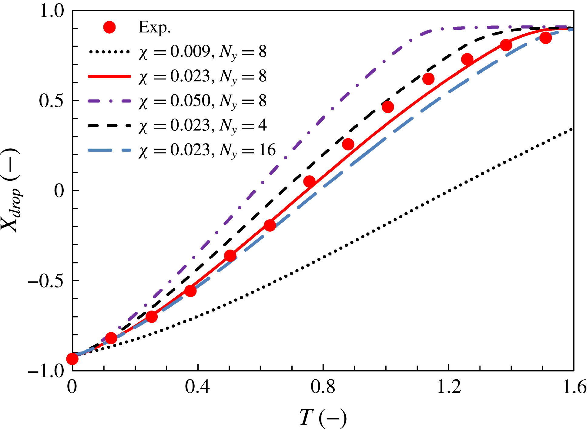
Position of droplet centre of mass with time for various values of slip parameter
 $\unicode[STIX]{x1D712}$
and resolution. Experimental data are from Lu et al. (Reference Lu, Glasner, Bertozzi and Kim2007).

4.5 Slip-parameter identification and grid-convergence tests
The non-dimensional slip parameter
 $\unicode[STIX]{x1D712}$
used in the GNBC front tracking can be estimated approximately using (4.3) and (4.4) with experimental values of
 $\mathit{Ca}_{drop}$
and
 $\unicode[STIX]{x1D703}_{dA}$
or
 $\unicode[STIX]{x1D703}_{dR}$
. However, the contact-line elements of the moving droplet move at various speeds depending on their position, so we must tune the parameter
 $\unicode[STIX]{x1D712}$
about its estimated value. Figure 4 shows the position of the droplet centre of mass with time for three values of
 $\unicode[STIX]{x1D712}$
with resolution
 $N_{y}=8$
, and grid resolutions of
 $N_{y}=4$
and 16 with
 $\unicode[STIX]{x1D712}=0.023$
. The position as shown has been shifted by
 $L_{x}/2$
and normalised by
 $R$
, and the time as shown has been normalised by
 $12\unicode[STIX]{x1D707}_{l}R^{3}/(\unicode[STIX]{x1D70E}b^{2})=2.12~\text{s}$
.
For large
 $\unicode[STIX]{x1D712}$
, the contact angle rapidly reaches the small static angle affected by EWOD, then the droplet moves away quickly. With
 $\unicode[STIX]{x1D712}=0.023$
, the simulation results coincide with the experimental data, hence we use this value hereafter.
In the grid-convergence tests, a higher resolution causes the droplet to move more slowly, which may be because the drag force is being evaluated more accurately. We can see the convergence tendency with grid resolution from figure 4. Although higher-resolution computation is desirable, we must use a cubic grid of the same size along every axis to avoid the effect of surface tension being distributed anisotropically, and this imposes huge memory demands. For higher resolution, a more suitable value for
 $\unicode[STIX]{x1D712}$
may be found. However, the difference of the results between
 $N_{y}=8$
and
 $N_{y}=16$
with constant
 $\unicode[STIX]{x1D712}$
is not so large and the variation of
 $\unicode[STIX]{x1D712}$
is almost proportional to variation of the droplet speed. So we consider that the suitable value of
 $\unicode[STIX]{x1D712}$
for large
 $N_{y}$
is not so greatly different from the
 $N_{y}=8$
case. Thus, we decided to use
 $N_{y}=8$
hereafter, which generally yields appropriate results.
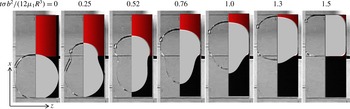
Composite images of moving droplet: simulations (right half of each panel) and experimental observation (left half of each panel), the latter from Lu et al. (Reference Lu, Glasner, Bertozzi and Kim2007).

Figure 5 shows composite images of a moving droplet simulated with
 $\unicode[STIX]{x1D712}=0.023$
and
 $N_{y}=8$
and paired with experimental observations. The left half of each panel is an experimental observation by Lu et al. (Reference Lu, Glasner, Bertozzi and Kim2007) whereas the right half is our simulation result. On the right-hand side, the grey region represents the (half) liquid droplet and the red (upper side) rectangle represents the positive electrode. Not only do the present simulations reproduce the droplet motion well (figure 4), they also capture the droplet shape very realistically (figure 5).
5 Discussion
5.1 Comparison of simulations with experiments and models
To evaluate the theoretical model described in § 3.1, we performed numerical simulations with various values of the shape parameters and calculated the non-dimensional droplet speed
 $\mathit{Ca}_{drop}$
. We calculated the speed of the simulated droplet while the centre-of-mass position changed almost linearly with time (for example in figure 4,
 $0.6\leqslant T\leqslant 0.9$
). To compare the present simulations with the theoretical model described in § 3.1, the dynamic effect of the contact angle in (3.2) can be replaced by (4.3) and (4.4). To simplify solving the simultaneous equations, we use the following relationship for the dynamic effect with the approximation
 $\unicode[STIX]{x1D703}_{d}\approx {\unicode[STIX]{x1D703}_{d}}^{micro}$
as
 $$\begin{eqnarray}\cos \unicode[STIX]{x1D703}_{d}=\cos \unicode[STIX]{x1D703}_{s}-\frac{1}{\unicode[STIX]{x1D712}}\mathit{Ca}.\end{eqnarray}$$
The relation between the empirical (3.3) and (3.4) and the above (5.1) is confirmed here. The difference is just the coefficient of
 $\mathit{Ca}$
, and the values of coefficients are
 $(k\sin \unicode[STIX]{x1D703}_{sA}/(3\unicode[STIX]{x1D703}_{sA}^{2})+k\sin \unicode[STIX]{x1D703}_{sR}/(3\unicode[STIX]{x1D703}_{sR}^{2}))/2=33$
and
 $1/\unicode[STIX]{x1D712}=43$
. We consider that they are approximately consistent with omitting the scale effect (4.4). If we use (5.1) instead of (3.2), equation (3.8) is rewritten as follows:
 $$\begin{eqnarray}F_{s}=\unicode[STIX]{x1D70E}W\left[\frac{cV^{2}}{2\unicode[STIX]{x1D70E}}+2\left(\cos \unicode[STIX]{x1D703}_{sA}-\cos \unicode[STIX]{x1D703}_{sR}\right)-\frac{\unicode[STIX]{x03C0}}{\unicode[STIX]{x1D712}}\mathit{Ca}_{drop}\right].\end{eqnarray}$$
We can then obtain the equation for the non-dimensional drop speed in the simulation as
 $$\begin{eqnarray}\mathit{Ca}_{drop}=\frac{\displaystyle \frac{cV^{2}}{2\unicode[STIX]{x1D70E}}+2\left(\cos \unicode[STIX]{x1D703}_{sA}-\cos \unicode[STIX]{x1D703}_{sR}\right)}{\displaystyle \frac{12\unicode[STIX]{x03C0}R^{2}}{bW}+\frac{\unicode[STIX]{x03C0}}{\unicode[STIX]{x1D712}}}.\end{eqnarray}$$
Droplet speed as a function of voltage. Experimental data are from Lu et al. (Reference Lu, Glasner, Bertozzi and Kim2007).

The dependency of droplet speed on voltage is shown in figure 6; equation (5.3) is also plotted in the figure. The simulation results agree well with the theory and part of the experimental data. For the experimental observations by Lu et al. (Reference Lu, Glasner, Bertozzi and Kim2007), equation (2.1) is only valid for
 $V\leqslant 60$
V. However, because our simulation model does not apply to the full range of (2.1), our simulation results do not agree with the experiment ones beyond
 $V=65$
V.
We varied the values of the shape parameters for the parametric study, with the channel width
 $b$
as 1/2, 2 and 3 times that in the base case (corresponding to
 $5.3\times 10^{-4}~\text{m}$
in the experiment by Lu et al. (Reference Lu, Glasner, Bertozzi and Kim2007)), the electrode size
 $W$
is 1/2, 3/4 and 5/4 times that in the base case (
 $1\times 10^{-2}~\text{m}$
), the droplet size
 $R$
is 5/4 and 3/2 times that in the base case (
 $5.5\times 10^{-3}~\text{m}$
) and
 $R$
and
 $W$
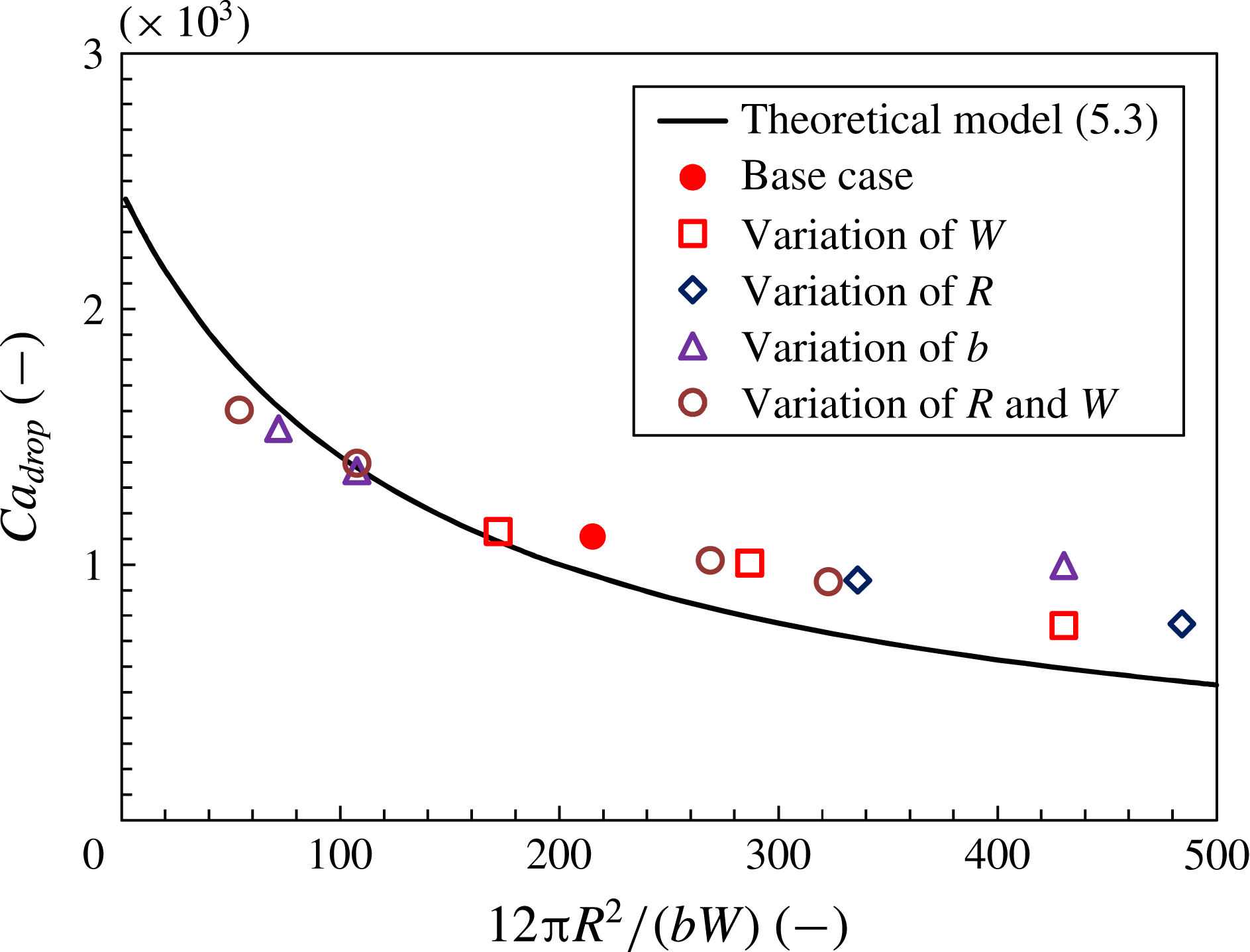
simultaneously are 1/4, 1/2, 5/4 and 3/2 times those in the base case. Figure 7 shows the simulated droplet speed against the theoretical relationship for the various shape-parameter values.
Comparison of simulated droplet speed with theoretical model.

For the smallest value of
 $b$
(the rightmost triangle plotted in figure 7 at
 $12\unicode[STIX]{x03C0}R^{2}/(bW)=430$
), there were only four grid points in the wall-normal direction, so the viscous drag could not be represented accurately and hence the droplet speed was not reproduced accurately. Except for this rightmost triangle, the simulated droplet speeds are aligned in a curve that agrees fairly well with the theoretical curve.
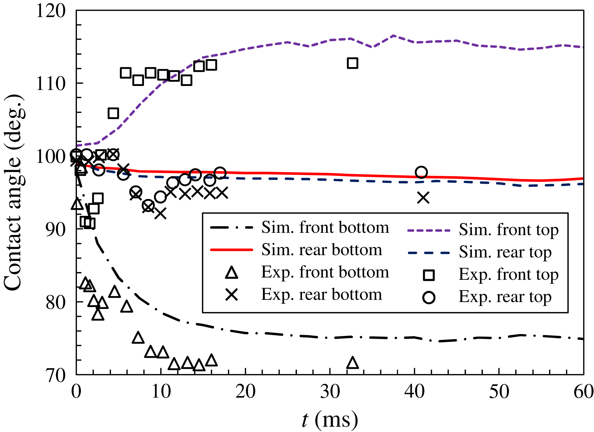
Temporal changes of contact angles of the droplet front and rear tips just after applying a voltage. Experimental data are from Lu et al. (Reference Lu, Glasner, Bertozzi and Kim2007).

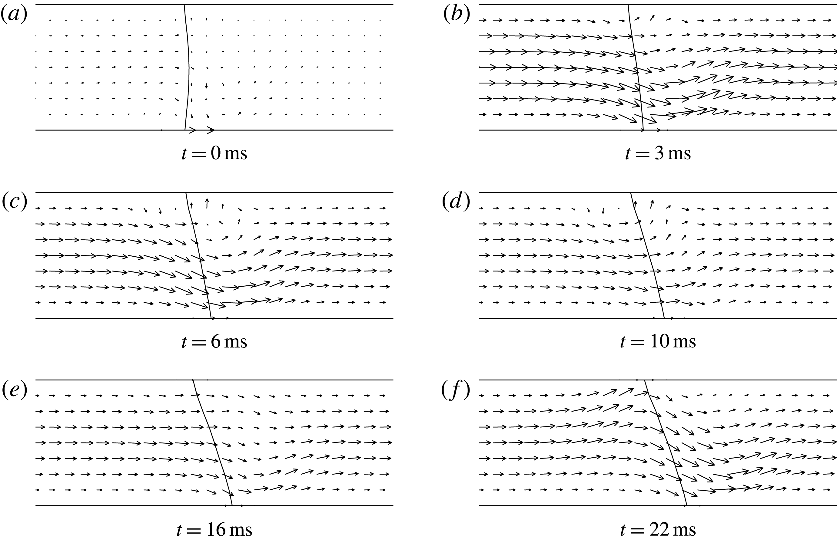
Velocity field and interface shape in the vertical centre plane near the droplet front just after applying a voltage.

5.2 Dynamics at the onset of motion
Figure 8 shows the temporal changes of the contact angles of the top/bottom menisci at the droplet front/rear just after applying a voltage. The contact angles in the present simulation were calculated with triangular elements, so the contact angle is the macroscopic one measured on the scale of
 $\unicode[STIX]{x1D6E5}$
. The angles measured experimentally by Lu et al. (Reference Lu, Glasner, Bertozzi and Kim2007) are also shown in the figure. The temporal behaviour of the simulated angles shows the same tendency as that of the experimentally measured angles. The measured value of the apparent dynamic contact angle is dependent on the observation scale, so the absolute values of the simulated angles do not coincide perfectly with the experimentally measured ones. The front-bottom contact angle, whose contact line lies on the positive electrode, decreases quickly according to (2.1). The front-top contact angle increases because of dragging by the wettable front-bottom contact line. The rear contact angles remain approximately constant at
 $98^{\circ }$
, close to the static receding angle as stated in § 3.2, because the rear contact lines are still at rest. From figure 8, the experimental data give a time scale of
 $T_{s}\sim 10~\text{ms}$
on which the contact angles reach their steady values, and this is reproduced in the simulations. Below, by analysing the simulation data, we consider a mechanical model that determines the time scale
 $T_{s}$
.
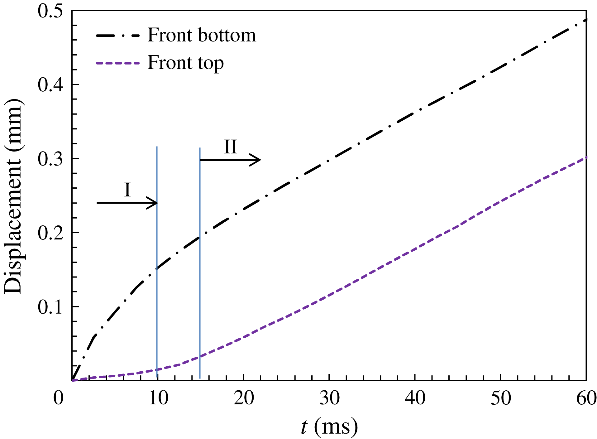
Displacement of droplet top and bottom front contact lines just after applying a voltage.

Figure 9 shows instantaneous shapes of the interface near the droplet front in the vertical centre plane obtained from the base-case simulation. The interface shape varies until
 $t\sim 10~\text{ms}$
and reaches an almost steady shape for
 $t\gtrsim 15~\text{ms}$
. The front-bottom contact line that is affected by electrowetting moves continuously, whereas the front-top contact line hardly moves until
 $t\sim 10~\text{ms}$
.
The displacements of both the top and bottom of the front contact line are shown in figure 10. We can divide the temporal behaviour of the contact lines approximately into two stages (I and II). In stage I (
 $t\lesssim 10~\text{ms}$
), the front-top contact line hardly moves whereas the front-bottom contact line moves with nearly constant speed (constant slope in this figure) as mentioned above for figure 9. In contrast, in stage II (
 $t\gtrsim 15~\text{ms}$
), both the top and bottom front contact lines move with the same speed, which is less than the speed of the front-bottom contact line in stage I. From figure 8, we can see that the contact angles in stage II are approximately
 $75^{\circ }$
(bottom) and
 $115^{\circ }$
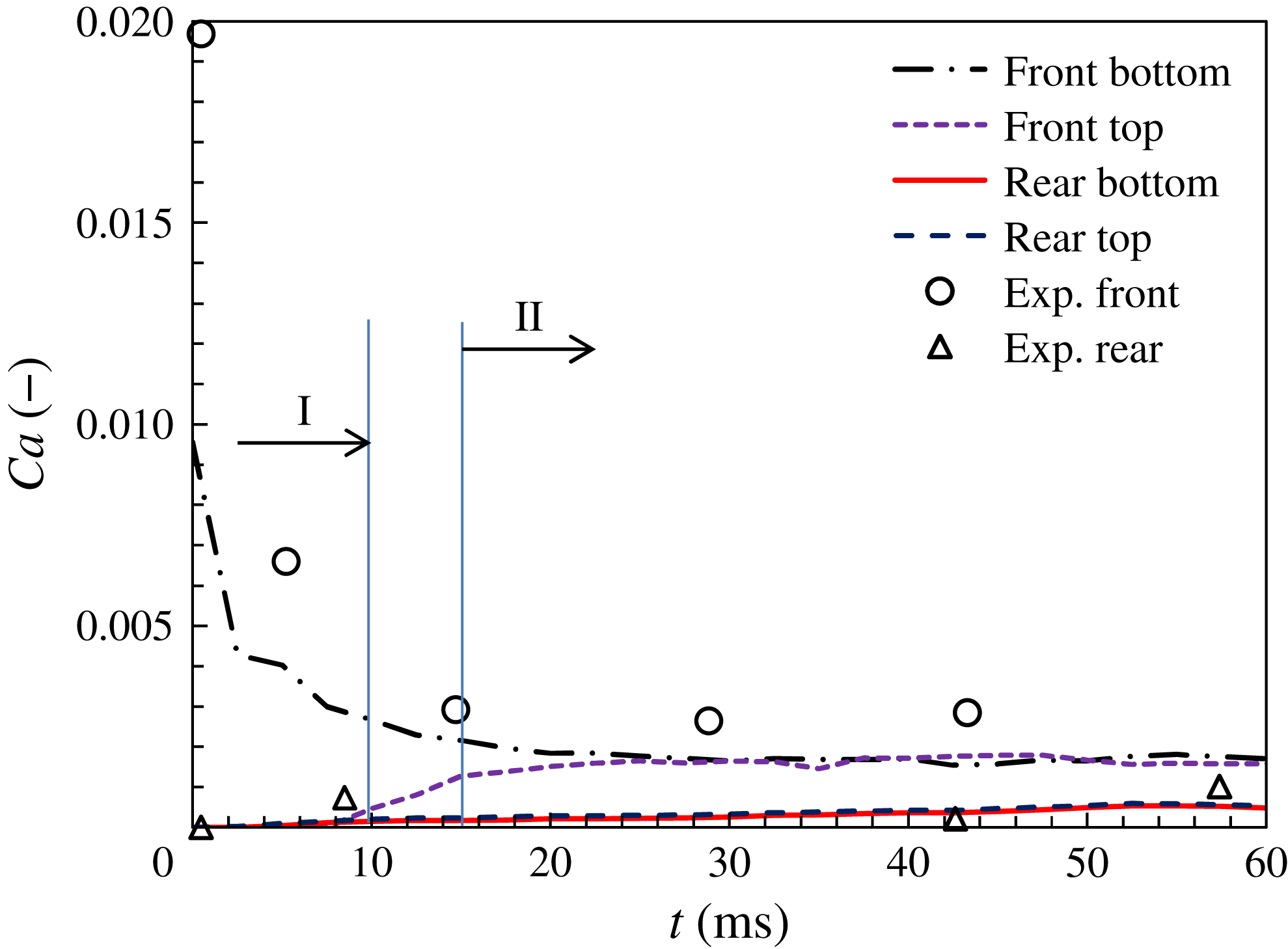
(top). Figure 11 shows the non-dimensional contact-line speeds
 $\mathit{Ca}$
of the droplet front and rear against those measured experimentally by Lu et al. (Reference Lu, Glasner, Bertozzi and Kim2007). In the first millisecond, the front-bottom contact line moves very quickly over the positive electrode. We can estimate this high speed (
 $\mathit{Ca}\approx 0.02$
) from (3.1) or (5.1) with the change in contact angle due to the electrowetting effect as given by (2.1) at
 $t=0$
. Subsequently, the speed decreases rapidly and reaches an approximately constant value at
 $t\sim 20~\text{ms}$
. In stage II (
 $15\lesssim t\lesssim 100~\text{ms}$
), the front contact lines move much more quickly than do the rear ones, with the latter being effectively stationary. Despite there being a dearth of experimental data for
 $t=1{-}10~\text{ms}$
, the contact-line behaviour in stages I and II, as shown in figures 10 and 11, corresponds to that shown in figure 8.
Non-dimensional speed (capillary number) of front and rear contact lines just after applying a voltage. Experimental data are from Lu et al. (Reference Lu, Glasner, Bertozzi and Kim2007).

Hereafter, we discuss the aforementioned contact-line behaviour shown in figure 11. Summarising the behaviour of the contact lines, in stage I, only the front-bottom contact line moves quickly and reaches a steady contact angle of
 $75^{\circ }$
, whereas in stage II, the front-top contact line starts to move with the same speed as the front-bottom one. After stage II, the rear contact lines start to move, then the entire droplet moves at constant speed as discussed in §§ 3, 4.5 and 5.1.
The time scale for boundary-layer development (i.e.
 $t_{b}\sim 0.3~\text{ms}$
as stated in § 3.1) is shorter than the 10 ms for the contact-line behaviour in stage I. In addition, we evaluate here the time scale
 $t_{s}$
on which the speed of the droplet centre of mass approaches the steady state. If we consider the familiar problem of terminal speed under the influence of a viscous drag that is proportional to speed,
 $t_{s}$
can be estimated approximately from the droplet mass divided by the velocity-coefficient part of the viscous drag:
 $$\begin{eqnarray}t_{s}={\displaystyle \frac{\unicode[STIX]{x1D70C}_{l}\unicode[STIX]{x03C0}R^{2}b}{\left({\displaystyle \frac{12\unicode[STIX]{x1D707}_{l}\unicode[STIX]{x03C0}R^{2}}{b}}\right)}}=\frac{\unicode[STIX]{x1D70C}_{l}b^{2}}{12\unicode[STIX]{x1D707}_{l}}.\end{eqnarray}$$
In this study,
 $t_{s}$
is estimated as 1.5 ms, which is much smaller than the time scale of stage I (10 ms). Hence, we reason that the droplet moves at an each constant speed in stage I after
 $t\sim 1.5~\text{ms}$
and stage II.
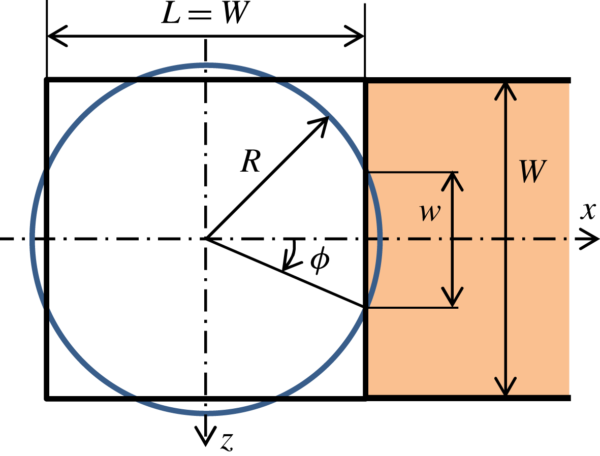
Schematic of initially circular droplet placed in the channel.

In stage I, surface tension is evaluated approximately by assuming only the front-bottom contact line moves. Figure 12 shows the geometry of an initially circular droplet with radius
 $R$
put in the channel. When a voltage is applied, only that part of the contact line over the positive electrode (width
 $w=2[R^{2}-(W/2)^{2}]^{1/2}$
as shown in figure 12) is subjected to EWOD. For this circular droplet, we may assume
 $\cos \unicode[STIX]{x1D719}\approx 1$
as shown in figure 12 because
 $R\approx W/2$
. Equation (3.8) for the surface-tension force acting on the droplet can then be rewritten as
 $$\begin{eqnarray}F_{sI}=\unicode[STIX]{x1D70E}w\left[\frac{cV^{2}}{2\unicode[STIX]{x1D70E}}+2\left(\cos \unicode[STIX]{x1D703}_{sA}-\cos \unicode[STIX]{x1D703}_{sR}\right)-\frac{\mathit{Ca}_{I}}{\unicode[STIX]{x1D712}}\right],\end{eqnarray}$$
where
 $\mathit{Ca}_{I}$
is the non-dimensional speed of the moving front-bottom contact line, defined as
 $\mathit{Ca}_{I}\equiv \unicode[STIX]{x1D707}_{l}U_{clI}/\unicode[STIX]{x1D70E}$
. Note that dynamic wetting affects only the contact line on the front part of the lower wall. In addition, we assumed in deriving (5.5) that the static receding contact angle could generate a resistant surface tension on the contact line excluding the front wall.
Now let us estimate the viscous drag. The average front speed is effectively half of
 $U_{clI}$
in stage I because the front-upper contact line stays still. In addition, the area of the moving part is approximated as
 $wW/2$
because the rear side of the droplet stays still. The viscous drag may then be estimated by using (3.12) for the velocity distribution:
 $$\begin{eqnarray}F_{vI}=2\frac{3\unicode[STIX]{x1D707}_{l}U_{clI}}{b}\frac{wW}{2}=\frac{3wW\unicode[STIX]{x1D70E}}{b}\mathit{Ca}_{I}.\end{eqnarray}$$
Equating (5.5) and (5.6), the non-dimensional contact-line speed
 $\mathit{Ca}_{I}$
in stage I is given as
 $$\begin{eqnarray}\mathit{Ca}_{I}={\displaystyle \frac{{\displaystyle \frac{cV^{2}}{2\unicode[STIX]{x1D70E}}}+2\left(\cos \unicode[STIX]{x1D703}_{sA}-\cos \unicode[STIX]{x1D703}_{sR}\right)}{{\displaystyle \frac{3W}{b}}+{\displaystyle \frac{1}{\unicode[STIX]{x1D712}}}}}.\end{eqnarray}$$
For stage II, a similar argument as above can be made. However, considering that both the top and bottom of the front contact line move while the rear side stays still, the surface-tension force can be determined as
 $$\begin{eqnarray}F_{sII}=\unicode[STIX]{x1D70E}w\left[\frac{cV^{2}}{2\unicode[STIX]{x1D70E}}+2\left(\cos \unicode[STIX]{x1D703}_{sA}-\cos \unicode[STIX]{x1D703}_{sR}\right)-\frac{2\mathit{Ca}_{II}}{\unicode[STIX]{x1D712}}\right].\end{eqnarray}$$
Also, the viscous force is given as
 $$\begin{eqnarray}F_{vII}=2\frac{6\unicode[STIX]{x1D707}_{l}U_{clII}}{b}\frac{wW}{2}=\frac{6wW\unicode[STIX]{x1D70E}}{b}\mathit{Ca}_{II}.\end{eqnarray}$$
We then obtain the non-dimensional contact-line speed
 $\mathit{Ca}_{II}$
in stage II as
 $$\begin{eqnarray}\mathit{Ca}_{II}=\frac{\unicode[STIX]{x1D707}_{l}U_{clII}}{\unicode[STIX]{x1D70E}}={\displaystyle \frac{{\displaystyle \frac{cV^{2}}{2\unicode[STIX]{x1D70E}}}+2\left(\cos \unicode[STIX]{x1D703}_{sA}-\cos \unicode[STIX]{x1D703}_{sR}\right)}{{\displaystyle \frac{6W}{b}}+{\displaystyle \frac{2}{\unicode[STIX]{x1D712}}}}}=\frac{1}{2}\mathit{Ca}_{I}.\end{eqnarray}$$
Substituting the parameter values used in this study into the above equations, we obtain
 $\mathit{Ca}_{I}=0.0034$
and
 $\mathit{Ca}_{II}=0.0017$
. The theoretical value of
 $\mathit{Ca}_{I}$
in stage I is less than the experimental value shown in figure 11, but the value of
 $\mathit{Ca}$
in stage I obtained by the present simulation (average over the stage) is almost the same as the theoretical one. In stage I, because the behaviour is transitional, a precise estimation is challenging and the present estimation is fairly good. The theoretical value of
 $\mathit{Ca}_{II}$
in stage II is also a good estimation for the present simulations and also roughly for the experiments.
For stage I, we can use (5.7) and (5.10) to estimate the time scale
 $T_{s}$
on which the contact angle reaches its steady state. Assuming that the shape of the interface changes from being up/down symmetric to flat with a lower contact angle of
 $75^{\circ }$
(figure 8), the displacement of the bottom contact line is estimated simply as
 $b/\tan (75^{\circ })$
. Dividing this by
 $U_{clI}$
in (5.7),
 $T_{s}$
is estimated as 13 ms, which coincides with the time scale shown in figure 8. As a result, the proposed simple consideration of contact-line dynamics can explain the time scale for the present dynamic change in contact angle.
6 Summary
Droplet movement by EWOD in a Hele-Shaw cell was analysed numerically and theoretically. The simulation method was constructed by using the Young–Lippmann equation to represent the EWOD and the generalised Navier boundary condition to represent the moving contact lines in the context of the front-tracking method. With an adjusted slip parameter, the present numerical simulations could reproduce well the shape evolution and speed of droplets observed experimentally. We also proposed a simple theoretical model for the droplet motion. The proposed model could describe well the voltage dependency of droplet speed below the saturation voltage as measured experimentally, and was verified by numerical experiments for various values of the shape parameters and voltage. We confirmed that the model could describe well the effects of shape and voltage on the droplet motion. Furthermore, the behaviour of the contact line at the onset of droplet motion as observed in our simulations and experimentally was analysed theoretically, and the time scale on which the contact angle changed was estimated very well.
Given that such time scale estimation is very important for the design and operation of microfluidic devices, we consider the theoretical model presented in this paper to be useful. Droplet deformation is very complex near the boundaries of electrodes, so the full three-dimensional numerical simulations presented in this paper will be useful for achieving more precise estimation. In future work, we intend to consider droplet splitting and merging.
Acknowledgements
This study was supported by JSPS KAKENHI grant no. 16K06095. The authors are grateful to K. Doi, K. Kikuchi and Y. Onishi for assistance with writing the EWOD simulation codes and grateful to Dr R. Otomo for fruitful discussions.