





1. Introduction
Radio transients are indicators of high-energy astrophysical processes in our Universe, and as such can probe extreme physics (e.g. Frail et al. Reference Frail, Kulkarni, Nicastro, Feroci and Taylor1997; Kramer et al. Reference Kramer2021). Coherent emitters such as pulsars and Fast Radio Bursts can be used to probe the interplanetary (Smirnov et al. Reference Smirnov2024), interstellar (Ocker & Cordes Reference Ocker and Cordes2026) and intergalactic (Macquart et al. Reference Macquart2020) media, yielding information about otherwise invisible matter, and indeed the cosmology of the Universe.
In recent decades, observations of the radio transient sky have moved from following up objects detected at high energies (e.g. Gehrels et al. Reference Gehrels2004) or wide-area optical surveys (e.g. Bellm et al. Reference Bellm2019), to blind surveys that select objects of interest in the radio (Murphy & Kaplan Reference Murphy and Kaplan2026). This builds on decades of work searching the fast (
 $\lt$
seconds) time domain for radio pulsars (e.g. Lorimer et al. Reference Lorimer2006) and Fast Radio Bursts (CHIME/FRB Collaboration et al. 2018), and epoch-to-epoch (
 $\sim$
years) comparisons of large radio surveys (e.g. Somalwar et al. Reference Somalwar2023). Historically, these searches have been insensitive to ‘medium’ timescales of a few seconds to a few hours. This has left a relatively unexplored space in the radio transient parameter space (Figure 1), which recent searches are beginning to fill.
Transient parameter space diagram of pseudo-luminosity against timescale. A representative distance of 5 kpc has been used to calculate the sensitivity of the survey (as the approximate distance of GPM J1839
 $-$
10, the first new transient detected by this survey). Shaded regions indicate those which this work explores via searches within 5-min observations (purple), 30–45-min pointings (cyan) and via images made several nights apart (orange). The lavender region indicates the parameter space that would be explored by processing the GPM data at full time resolution (0.5 s; see Section 4.4.2 for a discussion). Figure adapted from Rea et al. (Reference Rea, Hurley-Walker and Caleb2026).

Figure 1. Long description
A scatter plot representing the relationship between pseudo-luminosity and timescale for various astrophysical transients. The horizontal axis represents the timescale in GHz s, and the vertical axis represents the pseudo-luminosity in Jy kpc squared. The plot includes several clusters of data points representing different types of transients, such as fast radio bursts, radio magnetars, pulsars, and others. Shaded regions indicate the parameter space explored by different observation methods: purple for 5-min observations, cyan for 30-45-min pointings, and orange for images made several nights apart. The lavender region indicates the parameter space that would be explored by processing the data at full time resolution. Notable clusters include fast radio bursts in the upper left, pulsars in the lower left, and AGN/blazars in the upper right. The plot shows a wide range of pseudo-luminosities and timescales, with distinct regions for different types of transients.
Within this region lie recent serendipitous discoveries of unusual objects, such as the Galactic ‘burper’ (Hyman et al. Reference Hyman2005), extremely slowly rotating pulsars (Caleb et al. Reference Caleb2022), magnetic white-dwarf/M-dwarf binaries (Pelisoli et al. Reference Pelisoli2023), Main-sequence Radio Pulse emitters (Das & Chandra Reference Das and Chandra2021), the ‘Galactic Radio Transients’ (Anumarlapudi et al. Reference Anumarlapudi2026), and the ‘long-period radio transients’ (LPTs; Rea et al. Reference Rea, Hurley-Walker and Caleb2026). For the most part, these objects are coherent emitters that produce polarised radio waves and tend to be brighter at low to mid (100–1 000 MHz) radio frequencies. So far, these discoveries are confined to our own Milky Way galaxy.
It is thus timely to perform dedicated radio searches for transients in the image plane. Consistent and repeated observations are more valuable in placing meaningful limits on the activity and brightnesses of sources than heterogeneous searches (such as commensal use of other data, or archival searches). As the recently discovered sources are Galactic, observations over the Galactic plane could yield higher numbers of detected sources. The widest-area effort at mid frequencies is the Australian SKA Pathfinder (ASKAP; Hotan et al. Reference Hotan2021) Variables And Slow Transients survey, (VAST; Murphy et al. Reference Murphy2021), at 888 MHz. While most mid-frequency transient surveys (such as ThunderKAT; Fender et al. Reference Fender2016), suffer from the small fields-of-view that follow from using single-pixel feeds on dish-based telescopes (field-of-view
 $\theta\propto \frac{\lambda}{D}$
, where
 $\lambda$
is the observing wavelength and D is the dish diameter), ASKAP employs phased-array feeds to essentially widen the field-of-view by a factor of 36. To increase the field-of-view further, one can only decrease D (reducing sensitivity, only countered by increasing the number of dishes, leading to new computational challenges; see e.g. the Deep Synoptic Array; Hallinan et al. Reference Hallinan2019), or increase
 $\lambda$
.
Thus, low-frequency telescopes offer an effective view of the transient radio sky. For example, the LOw-Frequency ARray (LOFAR; van Haarlem et al. Reference van Haarlem2013) has been carrying out the LOFAR Two-metre Sky Survey (LOTSS; Shimwell et al. Reference Shimwell2017) of the Northern Sky; a search of just 2% of this data for transients revealed a new LPT (de Ruiter et al. Reference de Ruiter2024; de Ruiter et al. Reference de Ruiter2025). The Murchison Widefield Array (Tingay et al. Reference Tingay2013) is a low-frequency aperture array operating at Ilyarrimanha Ilgari Bundara, the CSIRO Murchsion Radio Astronomy Observatory. It is a precursor to the low-frequency component of the SKA Observatory and has been operating since 2013. Its flagship all-sky radio surveys, the GaLactic and Extragalactic All-sky MWA (GLEAM; Wayth et al. Reference Wayth2015) and GLEAM-eXtended (Hurley-Walker et al. Reference Hurley-Walker2022b) surveys have offered opportunities to search for radio transients across the entire Southern sky (Murphy et al. Reference Murphy2017; Hurley-Walker et al. Reference Hurley-Walker2022a; Horváth et al. Reference Horváth, Hurley-Walker, McSweeney, Galvin and Morgan2025), but with only a limited number of epochs.
In this work, we describe a new radio transient survey that leverages the wide field-of-view and Southern location of the MWA to regularly observe the Galactic Plane over 72 epochs in three campaigns spanning June 2022 to March 2025: the Galactic Plane Monitor (GPM). Section 2 describes the instrumental set-up and processing pipeline and resulting data products, Section 3 presents the detected transient objects, Section 4 discusses the effectiveness, limitations, and potential future utility of reprocessing the GPM, and Section 5 concludes with a summary and outlook.
Throughout, we use J2000 co-ordinates, and the convention that
 $\sigma$
refers to the local root-mean-square (RMS) noise of the dataset under discussion.
2. Observations and data processing
2.1 Observations
The Galactic Plane Monitoring survey was performed using the Phase II ‘extended’ configuration of the MWA, under project code G0080. The GPM was conducted over three observing semesters, described in Table 1.
Observation details for the three conducted epochs of the GPM. Not all observations could be searched for transients on all timescales due to ionospheric phase scintillation at low elevations (see Section 2).
 $\tilde{N_\mathrm{tiles}}$
indicates the median number of functioning tiles in the array during each epoch.

Pointing centres of the GPM over semesters 2022-A and 2024-A (blue), and 2024-B (lavender). Two pointings could not be scheduled and are shown in grey. The 20
 $^{\circ}\times20^{\circ}$
boxes shown are at the
 $\sim$
50% level of the MWA primary beam, relative to the maximum of each pointing centre. Detected transients described in Section 3 are overlaid with markers.

The MWA is capable of observing 30.72 MHz of instantaneous bandwidth placed within 72–300 MHz, with optimum instrumental sensitivity over 100–185 MHz. However, sky noise is dominant over the system temperature and is proportional to
 $\nu^{-2.7}$
(Rybicki & Lightman Reference Rybicki and Lightman1979), so similar noise levels are observed across 154–231 MHz when imaging (Hurley-Walker et al. Reference Hurley-Walker2017). The dispersive and scattering effects of the interstellar medium scale as
 $\nu^{-2}$
and
 $\nu^{\frac{-11}{3}}$
, respectively (Taylor & Cordes Reference Taylor and Cordes1993), and ionospheric phase shifts scale as
 $\nu^{-2}$
(Thompson et al. Reference Thompson, Moran and Swenson2001), with amplitude scintillation sometimes inducing extreme flux density fluctuations at the lowest frequencies (Waszewski et al. Reference Waszewski, Morgan and Jordan2022). These considerations might argue for as high an observing frequency as possible. However, the frequency range above 231 MHz is often contaminated with military satellites, and has a complex primary beam response with strong sidelobes (Cook et al. Reference Cook, Seymour and Sokolowski2021). To compromise between these competing effects, the GPM was performed using 185–215 MHz.
Galactic radio transients may produce time-variant emission on a range of timescales from less than a second (e.g. pulsars; Hewish et al. Reference Hewish, Bell, Pilkington, Scott and Collins1968) to many years (e.g. X-ray binaries; Markoff et al. Reference Markoff, Falcke and Fender2001). Detecting fast transients such as canonical pulsars and Fast Radio Bursts requires very high sampling rates such as provided by the Voltage Capture System (Tremblay et al. Reference Tremblay2015), as employed, for example, by the Southern-sky MWA Rapid Two-metre (SMART) pulsar survey (Bhat et al. Reference Bhat2023). High time and frequency resolution avoids smearing the short-duration (
 $\lesssim10$
ms) pulses and enables coherent correction of dispersive effects. This is impossible with standard correlator data, although some fast (
 $\sim$
0.5 s) signals can be recovered, such as interplanetary scintillation of compact radio sources (Morgan et al. Reference Morgan2018). Processing such fast timescales induces a large computational and data-handling challenge. The goal of the GPM is to detect long-period radio transients and other Galactic radio transients, so to compromise between time-resolution and computational cost, while still retaining the highest-resolution data in case of a detection, we perform the observations at 0.5 s resolution, but average them to 4 s for onward processing.
Formed by an analogue beamformer, the MWA primary beam is fixed on the sky for each observation, and the sky drifts through it, slowly changing the apparent flux density of radio sources. To minimise this effect, while still making each observation useful for detecting sources with pulses 30–60 s across, we integrate for 296 s per observation. The MWA-X correlator upgrade has enabled seamless transition between observations such that there are no flagged time-steps between observations (Morrison et al. Reference Morrison2023).
Ten pointings were selected to cover the largest fraction of Galactic volume visible to the MWA at night-time in semesters 2022-A and 2024-A. The centres of the pointings are set to
 $b=0^{\circ}$
, and span
 $300^{\circ} \lt l \lt 57^{\circ}$
in 13
 $^{\circ}$
intervals. Each pointing has an approximate full-width-half-maximum (FWHM) of 16–20
 $^{\circ}$
, varying somewhat with pointing position. This yields an overall coverage of
 $|b|\lt15^{\circ}$
and
 $284^{\circ}\lt l \lt73^{\circ}$
, with reduced sensitivity toward the edges. At
 $l\gt50^{\circ}$
, imaging artefacts from Cygnus A result in decreased sensitivity; close to the Galactic centre, the sky temperature is higher, and at lower Declinations, the primary beam sensitivity is decreased. For 2024-B, we scanned the rest of the Southern Galactic plane (despite the lower Galactic volume). Here we attempted a closer longitude spacing of
 $7^{\circ}$
, but some pointings could not be included in the schedule, leading to somewhat unequal spacing of the 11 successful pointings. Figure 2 shows the layout of the pointings as well as the detected transients (Section 3).
We found that at low elevations, strong ionospheric phase scintillation induced a large number of false positive detections on short (Section 2.3) to medium (Section 2.4) timescales, either by causing sources themselves to appear and disappear, or by affecting bright sources nearby, causing their sidelobes to appear as transients. In combination with the scheduling requirement to fit as many pointings as possible in the night-time available, in a sequential order in Galactic longitude, this effectively placed further longitude limits on the searchability of each semester, shown in Table 1.
Figure 3 shows an overview of the main stages of the processing described in the subsequent sections.
Diagram showing the data flow through the Galactic Plane Monitor transient search and deep mosaic creation. In each of the three epochs (2022-A, 2024-A, and 2024-B, there are M nights of observing (grey oblongs), each of which is internally composed of N snapshot observations (yellow boxes labelled ‘Obs’ in the diagram). M for each epoch is given in Table 1. Individual observations are searched for candidates (Section 2.3), catalogues from multiple observations pointed at a single location in a night are searched for transients (Section 2.4), and mosaics formed from a night of observations are also searched (Section 2.5). A subset of the highest-quality images from all three epochs is formed into a deep mosaic covering the entire GPM region (Section 2.6).

Figure 3. Long description
A diagram showing the data flow through the Galactic Plane Monitor transient search and deep mosaic creation. The diagram includes three epochs labeled as 2022-A, 2024-A, and 2024-B, each containing M nights of observing represented by grey oblongs. Each night is composed of N snapshot observations shown as yellow boxes labeled Obs. Individual observations are searched for candidates, and catalogues from multiple observations pointed at a single location in a night are searched for transients. Mosaics formed from a night of observations are also searched. A subset of the highest-quality images from all three epochs is formed into a deep mosaic covering the entire GPM region.
2.2 Imaging and calibration
The data were downloaded from the All-Sky Virtual ObservatoryFootnote
1
without calibration solutions applied, with RFI flagging performed by AOFlagger (Offringa et al. Reference Offringa, van de Gronde and Roerdink2012). We performed (phase and amplitude) calibration on dedicated pointings toward Hercules A, which at 200 MHz is
 $\sim377$
Jy (Hurley-Walker et al. Reference Hurley-Walker2017), sufficient to dominate the visibilities and produce good calibration solutions. We used the GLEAM-X pipeline (Hurley-Walker et al. Reference Hurley-Walker2022b) which incorporates this and other sources in the field to produce a sky model, then MitchCal (Offringa et al. Reference Offringa2016) to form complex antenna gains for each antenna, frequency, and polarisation. These were applied to all data for each night. Imaging was also performed with the GLEAM-X pipeline, using WSClean (Offringa et al. Reference Offringa2014) to create a continuum image of each 5-min snapshot (top-right panel of Figure 4). For speed, we decreased the clean thresholds to 5-
 $\sigma$
(peak detection) and 3-
 $\sigma$
(masked clean), as well as reducing the maximum number of major iterations to 3. Subtracting the deep visibility model formed in this process, the data are re-imaged at 4-s time resolution to produce a series of near-empty snapshots in which only transient and variable sources are visible (Hurley-Walker et al. Reference Hurley-Walker2022b; Horváth et al. Reference Horváth, Hurley-Walker, McSweeney, Galvin and Morgan2025), which are thence combined into a cube in 16-bit HDF5 format for compact storage and onward analysis, as described in Appendix B of Morgan et al. (Reference Morgan2018). An example slice of such a cube is shown in Figure 4, demonstrating that diffuse emission and point sources are subtracted well by the initial imaging process, despite reasonably significant ionospheric blurring effects in the displayed observation. Figure 5 shows the typical RMS as a function of Galactic longitude.
Examples of the four imaging products generated in this work, using the same region for reference. Top-left: a single slice from a continuum-subtracted time-step cube (Section 2.3); top-right: a single five-minute snapshot (Section 2.4); bottom-left: a night-long mosaic (effective integration time
 $\sim$
30 min: see Section 2.5); bottom-right: the deep mosaic formed with the ‘lucky imaging” approach (Section 2.6). The RMS noise of each image is, respectively, 110, 26, 14, and 5 mJy beam
 $^{-1}$
. All images except the bottom-right were generated from observations on 2022-06-30 at
 $\sim$
16h UTC. In each panel, a 15
 $^{\prime}$
square region around the LPT GPM J1839
 $-$
10 is highlighted, and displayed in the bottom-left insets. Within these, the PSF of each image is shown as white ellipse in the bottom-left corner.

Noise levels of the various data products formed in this work, as a function of Galactic longitude. The points show median values while the error bars indicate the 1st (lower) and 3rd (upper) quartiles. The formation of the cubes and snapshots is described in Section 2.2, and the mosaics in Section 2.5. The change in spacing of the observations over longitude is due to a combination of a change in pointing separation between 2022-A/2024-A (
 $13^{\circ}$
) and 2024-B (
 $7^{\circ}$
), with gaps resulting from unforeseen limitations in the scheduling (see Section 2.1 for details). The relatively high RMS of the mosaics at
 $l= 285^{\circ}$
is due to this region lying on the edges of both the GC and SP regions.

2.3 Intra-snapshot search
Individual observations are sensitive to transients on timescales between the imaged time resolution (4 s), to approximately half of the observation duration (
 $0.5\times 5$
min). To extract transients on these timescales from within five-minute snapshots, we used filter methods developed by Horváth et al. (Reference Horváth, Hurley-Walker, McSweeney, Galvin and Morgan2025) in their search of a subset of GLEAM-X data. Briefly, these consist of:
-
1. A sum of Gaussian matched-filters of 4, 8, 16, and 32 s widths;
-
2. A search for any pixel that has brightness
 $\gt$
7
$\times$
the local RMS of that voxel along the time axis;
-
3. A search for any voxel that has an RMS along the time axis larger than
$5\times$
the median value of other voxels in the image.


The ionosphere induces phase scintillation of radio sources over timescales of
 $\sim$
30 s, and this can produce a large number of false positives. To combat this, we excluded any candidate with a peak brightness equal to or less than a known radio source in the GLEAM catalogues (Hurley-Walker et al. Reference Hurley-Walker2017; Hurley-Walker et al. Reference Hurley-Walker2019), cross-matched within a 2
 $^{\prime}$
radius. The detection sensitivity of the latter catalogue, which covers
 $|b|\lt10^{\circ}$
, is similar to the per-snapshot sensitivity of the GPM data, and thus this cross-match performs efficiently.
Some observations still produced large volumes of candidates due to instrumental or calibration errors. Any observation that produced more than 10 candidate transients after the above ionospheric filtering was excluded from onward processing.
After selecting candidates that passed any of the three filters in acceptable observations, we produced light curves and animations of the surrounding
 $200\times200$
pixel (
 $45'\times45'$
) regions for visual inspection.
2.4 Inter-snapshot search
Each 30- or 45-min integration points within a few degrees of the same location in the Galactic plane (limited by the analogue beamformer), divided into 6–9 snapshot observations. Transients on timescales of the snapshot time (5 min) to the total integration time (30–45 min) can be detected by performing cross-matches of the source catalogues detected in these snapshots and performing some statistical tests.
We use Aegean v2.2.5Footnote
2
(Hancock et al. Reference Hancock, Murphy, Gaensler, Hopkins and Curran2012; Reference Hancock, Trott and Hurley-Walker2018) and its companion tools such as the Background and Noise Estimator (BANE) to perform source-finding, with the default settings. We use the flux_warp
Footnote
3
package (Duchesne et al. Reference Duchesne, Johnston-Hollitt, Zhu, Wayth and Line2020) applying a set of radial basis functions to bring the source flux densities into agreement with the GLEAM-X GP catalogue of Mantovanini et al. (Reference Mantovanini2025c), for
 $|b|\lt10^{\circ}$
and
 $233^{\circ} \lt l \lt 44^{\circ}$
, and GLEAM outside of this region (Hurley-Walker et al. Reference Hurley-Walker2022b). We use the fitted 200-MHz flux densities from these catalogues to best-match the observing frequency of the GPM.
We also apply fits_warp (Hurley-Walker & Hancock Reference Hurley-Walker and Hancock2018) to shift the radio source positions into agreement with higher-resolution radio catalogues. We used the Rapid ASKAP Continuum Survey (RACS; McConnell et al. Reference McConnell2020; Hale et al. Reference Hale2021) Low Data Release 1. These position shifts are typically
 $\sim$
1–10
 $^{\prime\prime}$
.
Using the Starlink Tables Infrastructure Library ToolSet (STILTS; Taylor Reference Taylor, Gabriel, Arviset, Ponz and Enrique2006), we perform a cross-match between all snapshot catalogues within a given pointing, using a 25
 $^{\prime\prime}$
cross-matching radius and keeping all matches, which allows us to retain non-detections (i.e. transients). This relatively large cross-matching radius is necessary due to residual ionospheric errors caused by small (
 $\sim$
degree-size patches) scale ionospheric defocussing, which cannot be corrected by fits_warp.
We then exclude from our catalogues:
-
• sources with extent (integrated to peak flux density ratio)
$\gt1.5$
in any image; -
• sources where Aegean failed to fit a shape in any image (usually artefacts or parts of extended structures such as supernova remnants);
-
• sources more than
$9.^{\circ} 5$
from the center of the combined pointings, where the coverage of the combined pointings is low and has high noise; -
• sources which are decomposed in any image into components lying within 2
$^{\prime}$
of each other.


Where a source is not detected in an image, we perform a forced photometric measurement at the location of the mean position obtained from images where the source was detected. We set the uncertainty on this flux density measurement to the local RMS noise measured by BANE at the same position.
Due to the limited number N of data points (6–9), we use the simplest transient search variability metrics: the significance of variability
 $\eta$
and the coefficient of variation V (McKay Reference McKay1932):
 \begin{equation} \eta = {\chi}^2_{N-1} = \frac{1}{N-1} \sum^N_{i=1} \frac{\left(S_{i}-\overline{S}^*\right)^2}{\sigma_i^2}\end{equation}
and
 \begin{equation} V = \frac{1}{\overline{S}} \sqrt{\frac{N}{N-1} \left(\overline{S^2} - \overline{S}^2\right)},\end{equation}
where
 $\overline{S}$
is the mean flux density, and
 $\overline{S}^*$
is the weighted average flux density, respectively. The standard error
 $\sigma_i$
on the ith flux density measurement
 $S_i$
is calculated as the quadrature sum of the local RMS noise and a 10 % flux density calibration error.
For sources which meet the following criteria:
-
•
$\eta\gt5$
; -
•
$V\gt0.5$
; -
• mean
$S/\sigma \gt 6$
, calculated using images in which the detection was made (i.e. not including forced measurements),


we generate a light curve and an animation of a
 $200\times200$
pixel (
 $45'\times45'$
) region around the source for visual inspection.
2.5 Mosaic search
Observing the same sky across multiple epochs also enables a search for radio transients that change between epochs, i.e. timescales of days to weeks. We use the flux-density calibrated primary-beam-corrected images where ionospheric position shifts have been removed, generated in Section 2.4. We then form weight images based on the inverse of the square of the RMS maps calculated by BANE. We noted that the primary beam correction had occasionally introduced artefacts into the edges of the images, so also cropped the outer 800 pixels (3.3
 $^{\circ}$
) of both the images and RMS maps. The RMS in these regions is typically
 $\sim100\times$
that of the centre part of the image, so very little useful data is lost.
We use the mosaicking software swarp (Bertin et al. Reference Bertin, Bohlender, Durand and Handley2002) to form a Cartesian FITS image in Galactic coordinates, weighting each 5-min snapshot by the weight images. The resulting images have RMS noise 7–25 mJy beam
 $^{-1}$
, largely depending on proximity to bright sources, around which calibration artefacts can be significant.
Night-time observations generally form good-quality images following this procedure, but daytime observations suffer significant direction-dependent time-dependent ionospheric effects, with the net effect producing significant smearing of the sources beyond the nominal point spread function. We therefore restricted our mosaicking to night-time observations. An example of the imaging quality obtained is shown in the bottom-left panel of Figure 4. Figure 5 shows the typical RMS of the mosaics within
 $|b|\lt10^{\circ}$
as a function of Galactic longitude.
To search for radio transients and variables, we performed a similar process to that described in Section 2.4. Several changes were made to the process to accommodate the large mosaics:
-
• due to their similar sky coverage, we searched all data from semesters 2022-A and 2024-A in one analysis;
-
• to account for point spread function (PSF) projection and ionospheric blurring without expending unnecessary effort in determining it exactly, we relaxed the extent constraint to
$\gt3$
; -
• instead of a pointing centre distance cut, we cut 150 pixels (36
$^{\prime}$
) from the edges of mosaics and any areas where the local RMS noise exceeded 200 mJy beam
$^{-1}$
(typically on the Northern edge where Cygnus A is a strong source in the primary beam sidelobes); -
• the source density in the mosaics is sufficiently high that imposing a 2
$^{\prime}$
‘isolation’ cut (as performed for the snapshots) can result in the exclusion of real transients, so we adjusted this to best recover transients while not including too many false positives from sources decomposing into multiple objects:-
− within the GC region, the calibration and imaging quality motivated a 112
$^{\prime\prime}$
radius and exclusion of groups size 2 or more; -
− the SP region had higher imaging and calibration quality enabling a 60
$^{\prime\prime}$
radius and the exclusion of groups of size 3 or more;
-
-
• as the image quality was generally higher in the mosaics than the snapshots, we reduced the cuts to select variable sources to:
-
−
$\eta\gt2$
; -
−
$V\gt0.3$
; -
− mean ‘on’
$S/\sigma \gt 5.5$
,
-


then inspected the candidates visually using light curves and animations, as per Section 2.4.
2.6 Deep mosaic
By combining our accumulated
 $\sim19\,000$
5-min snapshots with inverse-variance weighting, we can form a deep image of the Galactic plane at 200 MHz. Since in 2022-A and 2024-A a single calibration solution is applied for each night, and all individual snapshots are only relatively lightly-cleaned (Section 2.2), relative to the large amount of total integration time (
 $\sim320$
h), the resulting mosaics become dominated not by thermal noise, but by a combination of sidelobe and classical confusion, as well as calibration and imaging artefacts. Ionospheric blurring can occasionally be significant, which would increase confusion and decrease image quality if strongly affected snapshots were included in a mosaic.
We can therefore create the cleanest and deepest mosaic by taking a ‘lucky imaging’ approach, selecting only the most high-quality observations to be included. We determine this quality by cross-matching the source-finding results of each snapshot to a catalogue of unresolved sources as determined from the SUMSS and NVSS catalogues; from this subset we calculate the mean integrated to peak flux density ratio; we retain only snapshots where this ratio is
 $\lt1.25$
. This yields 2 953 snapshots to be mosaicked (
 $\sim$
15% of the total). We then perform the cropping, weighting, and mosaicking steps identically to Section 2.5, with a template covering the full spatial range of data taken from 2022 to 2025. A section of this image is shown in the bottom-right panel of Figure 4.
The mosaic does not have a well-defined PSF as it is formed from such a large range of snapshots, each of which has a unique PSF. This is in contrast to the GLEAM and GLEAM-X surveys, which were deliberately conducted in drift scan modes so that the PSF would be well-defined, and any residual difference between the measured PSF and expected PSF could be attributed to ionospheric blurring, measured, and corrected.
Since the GPM visibilities lack short baselines, and there exists already a deep 200-MHz mosaic specifically produced to reconstruct the multiple spatial scales of the Galactic plane (Mantovanini et al. Reference Mantovanini2025c), the utility of the mosaic formed in this work is mainly in measuring a slightly (
 $\sim2$
–3
 $\times$
) fainter point source population, as well as qualitatively revealing some of the fainter
 $\sim1'$
-scale filamentary structures in Galactic objects such as supernova remnants. This motivates a simplistic approach to characterising the PSF, wherein we simply measure it using unresolved sources, and do not attempt to correct for any ionospheric blurring. This is further supported by our ‘lucky imaging’ approach which should minimise the inclusion of ionospherically distorted data.
Following Hurley-Walker et al. (Reference Hurley-Walker2017) and (Reference Hurley-Walker2022b) we perform (
 $5\sigma$
) source-finding on this mosaic to produce an initial catalogue of 200-MHz sources. We use the RACS-Low 1 survey (Hale et al. Reference Hale2021) to determine which of these sources are unresolved and are therefore representative of the PSF. We concatenate the two Gaussian component RACS catalogues available from Vizier and select sources at
 $|b|\lt16^{\circ}$
to match our sky coverage. We then perform internal cross-match on this catalogue to remove all sources that have one or more neighbours within 45
 $^{\prime\prime}$
(the resolution of the GPM). We also apply Hale et al.’s criteria to select unresolved sources (see their Section 5.2.1), furthermore selecting only sources that are well-fit by one Gaussian (
 $Ng=1$
), and brighter than 15 mJy (equivalent to 50 mJy at 200 MHz, for a typical spectral index
 $\alpha=-0.8$
). We crossmatch this subset of the RACS catalogue with the initial GPM catalogue, further downselecting to sources in the GPM with
 $S_\mathrm{200\,MHz}/\sigma_\mathrm{200\,MHz}\gt10$
.
From this combined catalogue of isolated, compact sources, we create a PSF map following previously established methods (Hurley-Walker et al. Reference Hurley-Walker2017, Reference Hurley-Walker2019, Reference Hurley-Walker2022b). We average and interpolate the sources’ major axis
 $\theta_\mathrm{maj}$
, minor axis
 $\theta_\mathrm{min}$
, and position angle (PA) measurements, using Healpix (order
 $=5$
, i.e. pixels
 $\sim1 . \!\!^{\circ} 5$
on each side) as a natural frame in which to accumulate and average source measurements. These are projected on to a Galactic Cartesian grid for re-use. Figure 6 shows the final mosaic as well as the associated background, RMS noise, and PSF maps.
Deep mosaic and its ancillary data. From top to bottom: the deep mosaic, the RMS sensitivity map, the background map, the PSF major and minor axes, and the PSF position angle.

We then use the PSF map as an input to a final source-find using Aegean, this time using a seed-clip of
 $4\sigma$
and a flood-clip of 3
 $\sigma$
, subsequently discarding any source with a signal-to-noise of less than 4.5
 $\sigma$
. We discuss the characteristics of the resulting catalogue in Section 3.4.
3. Results
A summary of the detection results for each timescale is shown in Table 2. Here we examine each timescale in more detail.
3.1 Intra-snapshot search: Short-duration transients
By searching the model-subtracted timestep imaging cubes (described in Section 2.3), we detected 1 952 candidate transients across the three epochs of the GPM. All were visually inspected, and most originated from sidelobes around bright sources, the occasional bad frame in an observation, and aliasing from sources from outside of the field-of-view. Since the search covers a large number of (
 $\sim$
19 000 observations
 $\times$
4 000
 $\times$
4 000 quasi-independent pixels
 $\simeq3\times10^{11}$
) samples, and the noise is not completely Gaussian, we also detected 7–8-
 $\sigma$
candidates purely due to noise peaks.
Figure 7 shows all of the candidate transient pulses, with real transients identified and marked. Table 3 summarises the identified transients; all confirmed sources were detected at least three times. Two bright (
 $\gt30$
Jy) supernova remnants, SNR G21.8
 $-$
0.6 and SNR G326.3
 $-$
1.8, have sharp, distinct shell edges, that tended to ionospherically scintillate depending on the observing conditions. One compact (peaked-spectrum) radio source, NVSS J183537
 $+$
033151 demonstrated extreme variability in three adjacent observations in 2022-A (Figure A1(f)), with an (undersampled) variability timescale consistent with an episode of night-time interplanetary scintillation (not unknown at low frequencies; see e.g. Kaplan et al. Reference Kaplan2015). Two pulsars demonstrated detectable variability in 2024-B: PSR J0820
 $-$
4114 and PSR J0828
 $-$
3417. The former has been observed to null for about 30 s every few minutes (Johnston et al. Reference Johnston2021) while the latter is known to switch between ‘strong’ and ‘weak’ emission states (Esamdin et al. Reference Esamdin2005).
The main goal of the GPM was to detect LPTs, and in this respect each epoch successfully discovered a unique LPT. In 2022-A we discovered the LPT GPM J1839
 $-10$
(Hurley-Walker et al. Reference Hurley-Walker2023), that has been active for at least 33 years. Recent work by Horváth et al. (Reference Horváth2026) indicates that is likely to be a binary M-dwarf/white dwarf system, although the exact emission mechanism of the radio pulsations remains unknown.
In 2024-A, we detected multiple pulses from ASKAP J175534.9
 $-252749.1$
, originally discovered by Dobie et al. (Reference Dobie2024) as a single bright 2-min duration burst. Alongside dedicated follow-up, the GPM data confirmed this source as an LPT with a periodicity of 1.16 h (McSweeney et al. Reference McSweeney2025).
In 2024-B, we discovered the LPT GPM J0715
 $-11$
(McSweeney et al. in review), an LPT with a periodicity of
 $\sim8$
min, modulated by a 32.5-h activity window. The pulses from this LPT are sufficiently short (
 $\lt$
1 s) that Romer delay can be measured; combining this with optical observations, McSweeney et al. find that the system is consistent with a white dwarf pulsar in a 32.5-h orbit around a G-type star.
3.2 Inter-snapshot search: Medium-duration transients
Figure 8 shows the variability metrics
 $\eta$
and V for the isolated, compact sources identified as described in Section 2.4. 1 206 candidates passed the
 $\eta\gt5$
,
 $V\gt0.5$
, and
 $S/\sigma\gt6$
thresholds for visual inspection. Through this process, we identified 10 real transient or variable sources, shown in Table 4. The remaining candidates were largely caused by ionospheric phase scintillation and sidelobes from bright sources.
Detection statistics for the different timescale searches performed in this work. The final row does not include the edges of supernova remnants, as these should not be considered real transients or variables.

Candidates detected within 5-min observations in each epoch of the GPM, using the techniques described in Section 2.3. Real transients and variables, or the edges of supernova remnants that contaminate the results are marked and labelled, and are discussed in Section 3.1. LPTs are highlighted with gold stars, variable pulsars with red hexagons, and the single night-time IPS source with a grey square.

Five of the real transients are known pulsars, with relatively low dispersion measures (DM
 $\lt300$
pc cm
 $^{-3}$
) and typical periodicities
 $0.25 \lt P \lt 1.5$
s. Their light curves display variability without strong patterns, which is intrinsic and due to changes in their emission patterns. PSR J1853
 $+$
0505 and PSR J1717
 $-$
4054 in particular are well-studied nulling pulsars with multiple modes (Young et al. Reference Young, Weltevrede, Stappers, Lyne and Kramer2015). PSR J1703
 $-$
4851 has demonstrated two emission modes (Johnston et al. Reference Johnston2021), as has PSR J1107
 $-$
5907 (Wang et al. Reference Wang2020), while PSR J0846
 $-$
3533 demonstrates three (Wang et al. Reference Wang, Manchester and Johnston2007).
Mantovanini et al. (Reference Mantovanini2025b) recently measured the 72–231 MHz flux densities of 199 Galactic pulsars via mosaics integrating several hours of observing across two years. Their average flux densities at 204 MHz (the closest matching frequency to the GPM) are factors of
 $\sim2$
–
 $8\times$
lower than the maximum 200-MHz flux densities of the pulsars we measure in our analysis, consistent with the pulsars varying in their emission states. The detections of these pulsars are shown as red hexagons in Figure 8.
One of the detected transients is a candidate eclipsing binary millisecond pulsar. In the Evolutionary Map of the Universe pilot survey with the Australian SKA Pathfinder (Norris et al. Reference Norris2021), Zic et al. (Reference Zic2024) discovered ASKAP J164622
 $-$
440540, and the flux density measurements made with the GPM are analysed and published therein. They demonstrate that the absorption in the eclipsing phase is broader at low frequencies (as is expected for most eclipse mechanisms), and that the spectral index of the source (
 $\alpha=-2.7$
) is consistent with the millisecond pulsar population. The detections of this source are shown as green diamonds in Figure 8.
The remaining four sources detected in this search were long-period radio transients, shown as gold stars in Figure 8. Three are published sources; for ASKAP J175534.9
 $-$
252749.1 and GPM J1839
 $-$
10, the GPM was critical for determining the periodicity and other properties such as spectral index, scattering, and polarisation (Hurley-Walker et al. Reference Hurley-Walker2023; Dobie et al. Reference Dobie2024; McSweeney et al. Reference McSweeney2025, see also Section 3.1). ASKAP J183950.5
 $-$
075635.0 has not previously been detected at 200-MHz; indeed, only three days after this blind detection, follow-up observations with the MWA failed to reveal the source, despite a contemporaneous detection at GHz frequencies (Lee et al. Reference Lee2025). Unfortunately, there were no GHz measurements contemporaneous to this detection in the GPM, so it is not clear whether it is the spectrum or the brightness of the source that varied to the point where it changed its detectability between these two measurements.
ASKAP J172755
 $-$
343116 was detected blindly by the GPM as a double-peaked pulse across a 45-min integration at 2024-07-15 at 12:35 UTC (Figure B2(a)). It was also independently discovered by the VAST Collaboration using ASKAP. To date, only seven detections of this source have been made (including the one described here), yielding a preliminary periodicity estimate of 4.3 h (priv. comm. VAST collaboration). A forthcoming publication will investigate this source in further detail.
Compact objects blindly detected as variables or transients within the 5-min snapshots; see Figure 7 for their locations and Section 3.1 for discussion. Where possible, references for the sources’ original discovery and their most recent accurate position are given in the references column (in that order). The flux density at 200 MHz is calculated from its brightest appearance in all of the snapshots (Section 2.3; see Appendix A for plots). Uncertainties are dominated by the flux density scale error (10 %) but as these are all variable sources, the flux density is only indicative. The top part of the table shows known intrinsically-variable pulsars; the bottom section shows detections of long-period radio transients. Example light curves for each of these sources are shown in Appendix B.

Variability analysis for the 5–45-min timescale probed by comparing sources found in 5-min snapshots within a 30–45-min pointing (Section 2.4), using the metrics
 $\eta$
(Equation 1) and V (Equation 2). The grey contours are in log density, in order to indicate the location of the majority of non-variable sources (
 $\sim10^6$
objects). The coloured points indicate the 1 206 candidates that passed the
 $\eta\gt5$
(vertical line),
 $V\gt0.5$
(horizontal line), and
 $S/\sigma\gt6$
threshold for visual inspection. Red hexagons highlight pulsars, gold stars highlight LPTs, and the eclipsing binary MSP candidate is marked with a green diamond. Sources are detected multiple times, so these markers include both the detections of significant variability (within the top right region) and all other detections (elsewhere). Source details are shown in Table 4.

3.3 Mosaic search: Long-duration transients
Searching the mosaics via the methods described in Section 2.5 yielded 1 685 candidates; within these we detected 16 significantly variable astronomical objects: eight known pulsars, seven candidate or confirmed eclipsing binary millisecond pulsars, and the LPT GPM J1839
 $-$
10, which has been described in Sections 3.1 and 3.2. Table 5 summarises the sources detected via the mosaics and Figure 10 illustrates their variability statistics in context with the other sources. In the following sections, we discuss the two types of pulsars selected by this search and their variability characteristics.
3.3.1 Eclipsing binary millisecond pulsars
Four of these sources were blindly discovered by the GPM: PSR J1723
 $-$
3342, GPM J1734
 $-$
28, GPM J1752
 $-$
30, and GPM J1815
 $-$
14. These sources were followed up by Petrou et al. (Reference Petrou2025) with a range of observations, determining that the sources have negative spectral indices (
 $\alpha\sim-2.5$
) and
 $\gamma$
-ray source associations in the Fermi-LAT fourth source catalog data release 2 (4FGL; Abdollahi et al. Reference Abdollahi2020; Ballet et al. Reference Ballet, Burnett, Digel and Lott2020). After phase-folding the data, orbital periods of
 $\sim$
5–20 h are obtained; taken together, these attributes are consistent with newly-discovered eclipsing binary millisecond pulsars (MSPs). PSR J1723
 $-$
3342 has been successfully detected as an MSP with MeerKAT, and the other sources are subjects of an ongoing search for pulsations.
PSR J1740
 $-2650$
was identified by Frail et al. (Reference Frail, Mooley, Jagannathan and Intema2016) as a strong candidate binary MSP; phase-folding the GPM data resulted in the detection of an orbital period of 9.77 h, motivating follow-up observations with MeerKAT at inferior conjunction, resulting in the detection of a
 $P=$
1.83 ms pulsar (Hyman et al. Reference Hyman2025). As discussed in Section 3.2, ASKAP J164622
 $-$
440540 was also blindly detected in the GPM, independently discovered with ASKAP, and the GPM measurements for that source are published by Zic et al. (Reference Zic2024).
PSR J0955
 $-$
3947 was confirmed as a pulsar using MeerKAT observations by the TRAPUM project, who are carrying out a progressive campaign to search for radio pulsations from unassociated Fermi sources (Thongmeearkom et al. Reference Thongmeearkom2024). Folding the GPM detections on Thongmeearkom et al.’s published orbital period and phase-referencing to their time of ascending node yields a clear eclipsing pattern (Figure 9) similar to the pulsars seen in GPM data published by Petrou et al. and Zic et al.
Sources detected as variables in the 5–45-min searches. Where possible, references for the sources’ original discovery and their most recent accurate position are given in the references column (in that order). The flux density at 200 MHz is calculated from its brightest appearance in all of the snapshots (Section 2.4). Uncertainties are dominated by the flux density scale error (10%) but as these are all variable sources, the flux density is only indicative. The top part of the table shows known intrinsically-variable pulsars; the second section shows a candidate eclipsing binary MSP where clear eclipsing behaviour is noted. The bottom section shows detections of long-period radio transients.

3.3.2 Variable pulsars
Three of the pulsars identified as variable in the mosaics are known nulling pulsars: PSR J0828
 $-$
3417 is well-known to enter phases of producing bright bursts, followed by long windows of much fainter, more intermittent and bursty activity (Esamdin et al. Reference Esamdin2005; Burke-Spolaor et al. Reference Burke-Spolaor2012); PSR J1717
 $-$
4054 intermittently nulls on various timescales (Kerr et al. Reference Kerr2014); and PSR J1853
 $+$
0505 switches between three different emission states (Young et al. Reference Young, Weltevrede, Stappers, Lyne and Kramer2015). While the variability identified by our transient pipeline is consistent with the known behaviour of these pulsars, it offers little additional insight due to the long integration times of the data relative to the nulling timescales of the pulsars (as short as minutes) or indeed their spin periodicities (
 $\sim$
seconds).
Sources detected as variables in the mosaic searches. Where possible, references for the sources’ original discovery and their most recent accurate position are given in the references column (in that order). For all objects excepting the RISS detections, the timescale of variability (
 $=P_\mathrm{orb}$
for eclipsing binary MSPs) is sourced from the referenced papers. The flux density at 200 MHz is the average flux density of the source when it is blindly detectable in the mosaics, i.e. not including forced photometric measurements (Section 2.5). Uncertainties are dominated by the flux density scale error (10 %) but as these are all variable sources, the flux density is only indicative. The top part of the table shows non-eclipsing pulsars; the second section shows confirmed (prefixed by ‘PSR’) and candidate eclipsing binary millisecond pulsars; the bottom section shows detections of a long-period radio transient. Light curves for individual sources are shown in Figure 8.

Flux density measurements of PSR J0955
 $-$
3947 using night-long mosaics of GPM data, folded on the orbital period
 $P_\mathrm{orb}=0.387339$
days and time of ascending node
 $T_\mathrm{asc}=58097.44433$
(MJD) derived from MeerKAT timing data (Thongmeearkom et al. Reference Thongmeearkom2024). Orbit-dependent eclipses typical of absorption of radio pulses by material from an ablated companion are clearly visible. The unfolded data are shown in Figure C1(a).

Variability analysis for the days to months timescale probed by comparing sources found in integrated mosaics over several semesters of observing (Section 2.5), using the metrics
 $\eta$
(Equation 1) and V (Equation 2). The top panel shows the analysis for the mosaics in the semesters 2022-A and 2024-A, covering the Galactic Centre region; the bottom panel shows the analysis for the mosaics in semester 2024-B, covering the Southern Galactic Plane. The grey contours are in log density, in order to indicate the location of the majority of non-variable sources (
 $\sim10^5$
objects per panel). The coloured points indicate the 1 080 (top) and 605 (bottom) candidates that passed the
 $\eta\gt2$
(vertical line),
 $V\gt0.3$
(horizontal line), and
 $S/\sigma\gt5.5$
threshold for visual inspection. Red hexagons highlight variable pulsars, green diamonds highlight (candidate and confirmed) eclipsing binary MSPs, and the gold star highlights the single detected LPT. Source details are shown in Table 5.

The remaining five pulsars are not known to have changing emission states. The flux density variability measured by the GPM is more smoothly-varying and less stochastic, typified by small (
 $\sim10$
–30%) variations on timescales of weeks and sometimes larger (
 $\sim80$
–90%) variations on timescales of years (see Figure C2 for plots). Since these are all bright, relatively well-studied pulsars with no reported nulling behaviour, the observed variability in our data is likely to be caused by scintillation by the intervening interstellar medium.
Diffractive interstellar scintillation (DISS) has been measured for two pulsars in this group: PSR J1430
 $-$
6623 was measured by Johnston et al. (Reference Johnston, Nicastro and Koribalski1998) to scintillate on 93-s timescales at 660 MHz, and PSR J1559
 $-$
4438 was measured by Deller et al. (Reference Deller, Tingay and Brisken2009b) to scintillate on 77-s timescales at 600 MHz. Observations at lower frequencies should result in faster timescales of DISS (see e.g. Bhat et al. Reference Bhat2014), and this is therefore ruled out as the cause of the flux density variation on the observed long timescales for these two objects, and most likely for the other sources.
On the other hand, refractive interstellar scintillation (RISS) should produce flux density variations on timescales of 1–20 years at these positions (Hancock et al. Reference Hancock, Charlton, Macquart and Hurley-Walker2019), purely from the Earth’s relative motion. However, pulsars typically have velocities
 $O (100)$
km s
 $^{-1}$
(Hobbs et al. Reference Hobbs, Lorimer, Lyne and Kramer2005), a factor of a few greater than Earth’s relative velocity. This decreases the expected timescale of RISS to several weeks – a few years. This is consistent with the observed flux density variations of these pulsars (see Table 5 for a summary).
3.4 200-MHz catalogue
Source-finding on the mosaic yields a catalogue of 206 894 sources with a peak flux density to local RMS noise (signal-to-noise) value greater than 4.5. However, this includes some areas with poor-quality imaging, largely due to the sidelobes of bright sources. The 175 906 sources that lie within
 $210^{\circ} \lt l \lt50^{\circ}$
and
 $|b|\lt13^{\circ}$
are used for onward analysis in this section; the other 30 988 sources are made available, but marked in the catalogue (Table D4) as having low data quality and should be used with caution.
3.4.1 Astrometry
We cross-match the (high-quality subset of the) catalogue sources with the compact, isolated RACS catalogue used in Section 2.6 to correct the astrometry on a snapshot basis. Figure 11 shows the results, with the median offsets between the catalogues
 $\Delta\mathrm{RA}=-17\pm830$
mas and
 $\Delta\mathrm{Dec}=9\pm854$
mas; the uncertainties are 1-
 $\sigma$
(unweighted standard deviation) of the offsets in each direction. This is a lower uncertainty than the typical astrometric uncertainty of the RACS catalogue itself (
 $\sim2''$
), which is currently being updated to better-match the International Celestial Reference Frame (Duchesne et al. private communication).
Astrometric offsets of the final deep 200-MHz GPM catalogue from the RACS DR-I catalogue in RA and Dec. Source density is shown as an arbitrary colour axis. The upper and right histograms show the (unweighted) distributions of offsets in RA and Dec, respectively. The dashed lines show the median offsets in each direction (
 $\Delta\mathrm{RA}=-17$
mas;
 $\Delta\mathrm{Dec}=9$
mas).

Figure 11. Long description
Panel A: A heat map showing astrometric offsets in right ascension and declination. The x-axis represents the offset in right ascension in arcseconds, ranging from -2 to 2. The y-axis represents the offset in declination in arcseconds, ranging from -2 to 2. The color intensity indicates the source density, with higher densities shown in brighter colors. The central region has the highest density, with a gradient decreasing outward. Panel B: A histogram above the heat map showing the distribution of offsets in right ascension. The x-axis represents the offset in right ascension in arcseconds, and the y-axis represents the frequency of occurrences, ranging from 0 to 1000. The distribution is centered around 0 with a peak frequency. Panel C: A histogram to the right of the heat map showing the distribution of offsets in declination. The x-axis represents the offset in declination in arcseconds, and the y-axis represents the frequency of occurrences, ranging from 0 to 1000. The distribution is centered around 0 with a peak frequency. The dashed lines in both histograms indicate the median offsets in each direction.
3.4.2 Flux density scale, PSF, and noise properties
As discussed in Section 2.6, the flux density scale was matched to that of GLEAM-X: GP (Mantovanini et al. Reference Mantovanini2025c); to test whether this was successfully preserved through the mosaicking and source-finding, we cross-match again to the GLEAM-X: GP catalogue and present the measured flux density ratio as a function of signal-to-noise in Figure 12. We also test whether the PSF determination was successful by plotting the ratio of the integrated to peak flux densities as a function of signal-to-noise. There are no unusual trends and we conclude that the flux density scale is correctly matched, and the PSF is well measured.
Flux density ratio of the GPM catalogue to the fitted 200-MHz flux densities from GLEAM-X: GP (Mantovanini et al. Reference Mantovanini2025c), and the ratio of the integrated to peak flux densities (‘extent’) of the GPM catalogue, both plotted as a function of signal-to-noise in the GPM. The density of points is shown with an arbitrary linear colour scale. The horizontal line is drawn at a ratio of unity, where the source density is highest, as expected.

In Figure 13 we show the median and inter-quartile ranges of the RMS noise as a function of Galactic longitude. In general the noise is slightly lower than that of the GLEAM-X: GP catalogue, particularly around the Galactic Centre. However, this comes at the cost of poor recovery of diffuse emission (angular scales
 $\gtrsim2'$
).
Local RMS noise levels of the deep mosaic, compared to those of the 170–231 MHz source-finding image from GLEAM-X: GP (Mantovanini et al. Reference Mantovanini2025c). For each survey, the solid lines show the median values and the filled region spans the 25th and 75th percentiles (the 1st and 3rd inter-quartile ranges).

4. Discussion
4.1 Effectiveness of survey strategy
The original survey strategy of the GPM (epoch 2022-A) was formulated shortly after the discovery of the first LPT with the MWA (Hurley-Walker et al. Reference Hurley-Walker2022a). The goal was to survey the largest Galactic volume observable at night in that semester, with dwell times sufficient to find sources of that periodicity (18 min). At that time, the only other object that could guide the survey strategy was the Galactic ‘Burper’ (Hyman et al. Reference Hyman2005); their unifying feature being a transient activity window of order weeks to months, motivating continuous monitoring on at least a weekly cadence. Subsequently-discovered LPTs have periodicities longer than 18 min, and at least a handful of (mostly unpublished) examples have been seen to be active for less than two weeks (Rea et al. Reference Rea, Hurley-Walker and Caleb2026).
These factors potentially motivate a future survey strategy of integrating for longer (to pick up longer-period sources) and more frequently (to catch sources with a transient activity window). Of course, for a real telescope, there is only so much time available per night, and the only way to increase both of these terms is to increase the field-of-view of the instrument. This is difficult, as the MWA is already almost as wide-field as is practical at these frequencies; any wider and the deletorious effects of bright sources on the (chromatic) edges of the main lobe, and the computational cost of imaging extremely large fields-of-view, would become challenging. Forming multiple beams that avoid (null) bright sources and tiling a large area, potentially targeting areas of lower scattering, will be possible with the SKA-Low, and may be an effective way of increasing the yield of transient detections.
In the meantime, a complementary survey strategy in a future epoch of the GPM could be to perform longer tracks (
 $\sim4$
h) on particular Galactic longitude pointings, and iterate over the Galactic plane over the course of a week. This would start to fill in the unprobed parameter space indicated by the gap between the grey and red shaded regions in Figure 1. It would have the added advantage of being more likely to clearly detect ingress and egress of eclipsing binary millisecond pulsars, which are otherwise only selected by having highly variable light curves. The orbital periods derived therefrom would be far more accurate; the 2022-A GPM epoch enabled the detection of several new eclipsing binary MSPs (Table 5) but the initial periodicities determined from those initial 18 epochs were incorrect, and only converged on consistent periodicities once follow-up was performed (Petrou et al. Reference Petrou2025) and more samples were obtained in 2024-A.
Northern (
 $l\gt40^{\circ}$
) pointings were not effective uses of observing time due to the low primary beam sensitivity and the challenge of Cygnus A, and could be dropped from future observing. The spacing of
 $13^{\circ}$
in longitude was sufficient and easier to schedule than
 $7^{\circ}$
so would be a good choice to maintain over the Galactic plane.
Reflecting on the spatial distribution of the detected transient and variable objects (Figure 2), it is clear that despite the higher Galactic scattering expected at low Galactic latitudes, the yield of new eclipsing binary MSPs and LPTs was highest towards low Galactic latitudes, and especially around the Galactic centre. This is perhaps surprising since these areas are some of the most intensively surveyed by existing pulsar and transient surveys, but clearly the low-frequency image-domain searches pursued in this work have accessed a new population that is not well-selected by other searches: these sources are faint at high frequencies, and produce emission on long timescales which are selected against by the short dwell times and fast-transient oriented processing backends of most Galactic surveys.
Nevertheless, the GPM is very unlikely to detect any further eclipsing binary MSPs (or other well-known objects such as nulling pulsars, or ‘persistent’ LPTs; Hurley-Walker et al. Reference Hurley-Walker2023) at its current sensitivity levels. Potentially, the MWA Phase III upgrade, with a full 256 tiles correlated (Tingay et al. in review), could more than double the sensitivityFootnote
4
since only
 $\sim100$
tiles were functioning during the GPM observing (Table 1). Given most of the ‘new’ tiles in Phase III are in a centrally-condensed core that would generate mostly relatively short baselines, care would need to be taken to select the correct imaging parameters in order to remove or properly-deconvolve the diffuse emission in the Galactic plane, that could otherwise complicate onward source association and transient detection. Indeed, doubling the sensitivity would reveal more than double the number of sources, exponentially increasing the challenge of source association, perhaps requiring better calibration, and better treatment of ionospheric effects, than undertaken in this work.
Regarding ‘transient transients’ such as LPTs, further epochs are of course potentially able to find further examples, should they become active. This would need to be weighed against the processing costs of running such searches, as well as the potential of exploring other areas of sky. As shown by Figure 1 of Rea et al. (Reference Rea, Hurley-Walker and Caleb2026), several LPTs lie at relatively high Galactic latitudes, so even if the yield is low, a comprehensive search of both the MWA archive, and a new survey exploring a wide area of high-latitude sky, could be effective methods for finding new LPTs. Potentially, LPTs (or transients on similar timescales) could exist and be detectable at extragalactic distances (e.g. Anpilogov & Tyul’bashev Reference Anpilogov and Tyul’bashev2026); if so, they will be rare, and will require the search of large volumes of (preferably high-latitude) data. Efforts in these directions are currently underway.
4.2 Effectiveness of detection methods
Unusually for most transient surveys (Murphy & Kaplan Reference Murphy and Kaplan2026), the GPM explores a very large range of timescales, ranging from 4 s all the way up to several years, in a relatively well-distributed way (Figure 1). This descends from the employment of three different detection methods that sample multiple timescales. Since, effectively, ‘single-pulse’ searches were employed, this naturally leads to lower noise (better sensitivity) on the longer timescales (Figure 13).
Importantly, this leads to the question: could we make better use of our data? For example, every transient imaging cube is searched in isolation. However, periodicity (folding) searches for LPTs could stack the data over relatively long integrations per phase bin, potentially revealing faint, periodic sources, below the ‘single-pulse’ threshold. Such searches could be computationally expensive and would require barycentring, but are not infeasible. For a typical cube RMS noise level of 100 mJy beam
 $^{-1}$
at 4 s resolution (Table 1), the RMS noise from using all
 $\sim27$
h of integration per pointing in 2022-A and 2024-A would be 20
 $\sqrt{\frac{P_\mathrm{fold}}{\mathrm{1\, h}}}$
mJy beam
 $^{-1}$
; modulo, this only applies if the LPT is persistently active over the duration of the folded data. Potentially, returning to the visibilities may be even more effective, albeit computationally more challenging (Zic et al. in preparation).
On the longer timescales, we currently treat every pointing separately in the inter-snapshot searches, leading to very sparse light curves, particularly for the 2022-A and 2024-B epochs (30-min integrations). Combining the data across multiple pointings and employing more sophisticated statistics than
 $\eta$
and V may yield further transients. Andersson et al. (Reference Andersson2025) compared the use of these simplistic metrics with both citizen-science and generic feature classification approaches and found the latter were far more effective in finding real transients. Similar approaches here, necessarily dealing with the large gaps in sampling, may be effective.
4.3 Detections of radio transients
In this section we discuss the selection biases of the GPM in detecting objects of different classes. Figure 14 shows a Venn diagram of intrinsically variable objects (i.e. not due to scintillation) detected by the GPM, as a function of the three different detection methods employed.
Venn diagram of the different transients and variables detected in this work depending on their detection method.

4.3.1 Eclipsing binary MSPs
The eclipsing binary MSPs are unsurprisingly most easy to discover via the mosaic searches; only ASKAP J1646
 $-$
44 is bright enough, with a sharp enough ingress/egress, to detect within a single 30–45-min pointing (Figure B2(e)). What is perhaps most surprising is the lack of detections of any known eclipsing binary MSPs; PSR J0955
 $-$
3947 is the only exception to this and was only recently-discovered (Thongmeearkom et al. Reference Thongmeearkom2024). This indicates that the GPM survey is sampling a very different population than that sampled by traditional blind pulsar timing searches. The detected systems are likely more highly absorbed (i.e. in closer orbits, with more vigorous ablation of the companion star leading to higher material density), potentially in shorter-period orbits (high acceleration can be challenging for traditional pulsation searches), and will likely have high orbital inclination angles with respect to our line of sight. However, the non-detection of these systems may also point to at least some of them having eclipse durations and depths that are so long at low frequencies, they are rendered entirely invisible to our survey. A careful cross-match of all of our sources (not just those detected as variable) with existing pulsar catalogues could separate these different populations and effects.
The GPM is a blind survey, but after discovery, all of these sources were found to have
 $\gamma$
-ray associations. For several decades, various groups have observed the unassociated Fermi-LAT sources to search for pulsations, including these objects (e.g. Camilo et al. Reference Camilo2015; Clark et al. Reference Clark2023). That none were previously detected likely indicates that either the dwell times of these searches were too low, resulting in too low a chance of catching the sources out of eclipse, or the frequency of the observations was too low, such that the ablated companion material dispersed or absorbed the pulsations to the point of undetectability (both effects are stronger at low frequencies; Thompson et al. Reference Thompson, Blandford, Evans and Phinney1994). A further complicating factor is the poor localisation of the Fermi sources; for example, the nearest Fermi source to GPM J1734
 $-$
28 is 4FGL J1734.5
 $-$
2818, 11
 $^{\prime}$
away (c/f the
 $\sim5'$
Fermi localisation; Petrou et al. Reference Petrou2025). It seems more likely that the current
 $\gamma$
-ray localisation is incorrect than there be an even fainter
 $\gamma$
-ray source closer by. A radio timing campaign for the GPM-discovered MSPs is currently underway; constrained radio timing will enable
 $\gamma$
-ray timing which could conclusively determine an association. In the meantime, our results may motivate longer-dwell-time pulsation searches toward more spatially-separated radio source associations (ideally in combination with other metrics, e.g. compactness and spectral index; Frail et al. Reference Frail2018). This can require a challenging amount of observing time due to the small fields-of-view of radio telescopes operating at higher frequencies, which are necessary to defeat scattering and absorption effects.
4.3.2 Variable pulsars
Seven intrinsically variable pulsars were detected by the GPM, across all search methods employed. Perhaps surprisingly, the intra- and inter-snapshot searches found no sources in common, whereas the mosaic searches detected pulsars in common with the other two methods. This is particularly noticeable for PSR J0828
 $-$
3417, which displays very high variability on timescales of seconds (Figure A1(b)) when active, but also nulls for hours to days (Figure A1(a)). It was observed by 30 different pointings of the GPM but none caught a transition from the null state to active state. This underscores the importance of exploring multiple timescales of variability for maximum return.
Image-plane variance searches for pulsars are an emerging method; e.g. Ahmad et al. (Reference Ahmad2025) imaged multiple timesteps of the EMU survey and looked for high-variance sources, likely compact and scintillating and thus potentially previously undiscovered pulsars. This is a similar approach to the cube analysis performed here, but without the initial field subtraction step. At the current sensitivity levels (
 $\sim$
100 mJy beam
 $^{-1}$
) of the GPM, such searches are exceedingly unlikely to find pulsars that have not previously been discovered by traditional time-domain searches, particularly at these low and well-searched Galactic latitudes. However, higher latitudes offer more potential; the image-plane search over
 $\sim$
1 h of integration and 10 000 sq. deg. of GLEAM-X data performed by Horváth et al. (Reference Horváth, Hurley-Walker, McSweeney, Galvin and Morgan2025) discovered a very bright Rotating RAdio Transient (RRAT), described in full by McSweeney et al. (Reference McSweeney2025). Deeper and longer-integration searches may yet yield results, although widefield beamforming searches such as the SMART survey (Bhat et al. Reference Bhat2023) are more likely to be more successful in finding standard pulsars due to the large sensitivity boost of pulsar gating.
We also blindly detected five known pulsars via their RISS (Section 3.3, Table 5). This is not an efficient search method for new pulsars at low frequencies due to the very long timescales that need to be monitored. However, the GPM mosaic measurements could be used to constrain RISS from other pulsars. For example, cross-matching the GPM mosaic candidates (before any selection on
 $\eta$
or V) with the ATNF pulsar catalogue (Manchester et al. Reference Manchester, Hobbs, Teoh and Hobbs2005),Footnote
5
for those pulsars with measured 400-MHz flux densities (as a proxy for being visible at low frequencies) yields 136 matched objects. In combination with other measurements, the degree of RISS in the GPM may help constrain the turbulent electron content of our Galaxy.
Additionally, traditional pulsation searches often ignore the total flux density of pulsars on timescales longer than the observation, with a focus usually only on distinguishing between various emission states identified by changes in pulse profile shape. Potentially, examination of the GPM data toward the cross-matched pulsars might identify mode-switching pulsars via sharp changes in flux density, which could motivate further pulsation observations to determine what those states are.
4.3.3 Long-period radio transients
The science motivation of the survey was to detect new long-period radio transients, in particular to employ the intra-snapshot search methods developed by Horváth et al. (Reference Horváth, Hurley-Walker, McSweeney, Galvin and Morgan2025) specifically on the Galactic plane, where in theory the source density should be highest. All three methods successfully recovered LPTs, with the mosaic search being (unsurprisingly) least sensitive and only capable of detecting the brightest source, GPM J1839
 $-$
10.
The two longest-period sources, ASKAP J1727
 $-$
34 (
 $P\sim4$
h) and ASKAP J1839
 $-$
07 (
 $P\sim6$
h), were only detected once each, in the inter-snapshot search, and both have become dimmer since discovery (priv. comm. VAST collaboration). This is similar behaviour to the first LPT discovered with the MWA, GLEAM-X J1627
 $-$
52, which was only detectable for three months in 2018. However, this source had a much faster period of 18 min, rendering it much more likely to be detected. As discussed in Section 4.1, this ‘transient transient’ behaviour motivates continuous, repeated monitoring of the Galactic plane, with dwell times longer than those accomplished by the GPM and better-matched to this long-period population.
One hope for monitoring the Galaxy in a consistent and homogeneous way was the possibility of producing population-level measurements or limits on such sources, even if the detection rate was low. However, over the time that the GPM has been running, various new LPTs have been discovered, several of which are not visible at 200 MHz, potentially due to absorption along the line-of-sight, but also potentially due to intrinsic emission properties. The detection of ASKAP J183950.5
 $-$
075635.0 in this work, yet its non-detection a few days later during contemporaneous monitoring (and detection) at higher frequencies, demonstrates that either the brightness or spectral index of these sources can change dramatically. Coupling that with extremely variable windows of emission (from weeks to decades) and a wide range of periodicities, and the detection of further modulating periodicities in some sources (e.g. Horváth et al. Reference Horváth2026), there are too many possible variable parameters for the non-detections in the GPM to be particularly constraining. At best, we can suggest a rate of
 $\sim0.1$
LPTs per month per 1 000 sq. deg. of Galactic plane monitoring using the strategies pursued here, with avenues for improvement in survey strategy largely discussed in Sections 4.1 and 4.2.
4.4 Future processing
4.4.1 Polarisation
The searches described in this work were carried out in Stokes I, but the MWA observes in full polarisation, and has been used to measure the polarisation properties of both LPTs (Hurley-Walker et al. Reference Hurley-Walker2022a) and flare stars (Lynch et al. Reference Lynch, Lenc, Kaplan, Murphy and Anderson2017). Blind linear polarisation searches are (currently) computationally infeasible as the effects of Faraday Rotation from the magnetic interstellar medium would need to be corrected, necessitating costly frequency-domain imaging and Rotation Measure (RM) trials. Circular polarisation (Stokes V) is a viable search method, resulting in decreased sky noise and much-reduced clean ing requirements due to the dearth of circularly-polarised sources casting sidelobes across the imaged field-of-view. For instance, Lenc et al. (Reference Lenc, Murphy, Lynch, Kaplan and Zhang2018) reprocessed the 170–231 MHz part of the GLEAM survey over 30 900 sq. deg. to produce a southern-sky Stokes V survey, blindly detecting 14 pulsars and 6 artificial satellites. At mid-frequencies, circular polarisation searches are revealing new populations of highly scattered and faint pulsars (Sengar et al. Reference Sengar2025a, Reference Sengarb). Stokes V can also detect novel transients (Wang et al. Reference Wang2021). This motivates testing the utility of reprocessing the GPM data in Stokes V.
A brief initial investigation of the GPM data found that Stokes V imaging reduces noise levels in the resulting mosaics by 30%, and the snapshots by 50%, while the noise levels of the cubes are largely unaffected (Y. Low, Hons thesis, Curtin University). This implies that the continuum subtraction is already very effective at reducing the noise to approximately thermal limits in the transient cubes, but that the snapshots are highly dominated by imaging and calibration artefacts, and the mosaics somewhat less so (consistent with what is seen in Figure 4).
For 100% circularly-polarised sources, these sensitivity improvements would directly result in improved detection statistics. However, most pulsars and LPTs have only fractional (
 $\sim$
1–50%) circular polarisation, which would decrease the utility of such searches. Stellar bursts can be very highly circularly-polarised, but are also likely to be much fainter than the noise levels achieved by the GPM, the noise budget of which is dominated by the high sky temperature towards the Galactic plane and (relatively) low number of functioning tiles. Localisation of such bursts would also be extremely challenging given the arcminute spatial resolution of the survey and the high stellar density at low Galactic latitudes. For serendipitous novel transients, there is still potential in reprocessing the data. However, these polarisation search techniques may be better employed at higher latitudes in other upcoming MWA surveys.
4.4.2 Full time resolution
To make the computation of the GPM feasible, and to quickly achieve our primary goal of detecting LPTs with 30–60-s long pulses, the processing described in this work was undertaken at 4-s time resolution (Section 2.2). The discovery of GPM J0715
 $-$
1142, the pulses of which are only
 $\sim$
1 s long, potentially motivates a reprocessing of the data at full time resolution (0.5 s). Obviously, this would impose a factor of 8 increase in the cost of most processing tasks, particularly imaging. The noise levels of the individual time-steps would also increase by a factor of
 $\sqrt{8}\sim2.8$
which would need consideration as to whether it is worth the increased cost. A search for short-duration pulses could also motivate de-dispersion of the data, and we briefly examine the main considerations here.
We consider a pulse of duration 0.5 s observed across the 185–215 MHz bandwidth, and calculate that at a DM of 44 pc cm
 $^{-3}$
, it would be reduced in S/N by the above factor of 2.8 (i.e. would not be any more detectable without dedispersion at 0.5-s time resolution than in our current 4-s search). Sources of higher DM would be commensurately more affected. However, interstellar scattering is strong at low frequencies and could still render such sources undetectable even with de-dispersion. Bhat et al. (Reference Bhat, Cordes, Camilo, Nice and Lorimer2004) determined an empirical correlation between DM and scattering timescale which we use as a model (their Equation 7). At DM
 $=$
245 pc cm
 $^{-3}$
, the scattering timescale reaches 0.5 s. Thus, if image-plane dedispersion techniques are used, they would only improve the signal-to-noise of a subset of sources with narrow (
 $\lesssim4$
-s) pulses, within a DM range of
 $\sim44$
–245 pc cm
 $^{-3}$
.
Implementations of such techniques exist (e.g. Anderson et al. Reference Anderson2021; Di Pietrantonio et al. Reference Di Pietrantonio, Sokolowski, Harris, Price and Wayth2026, or the LOfar Radio Dedispersion SoftwareFootnote
6
) and typically utilise GPUs for rapid computation. Potentially, the more expensive stage of the processing would be generating the multi-channel images required to perform the dedispersion. For a 0.5 s pulse at DM
 $=$
245 pc cm
 $^{-3}$
, the 24 MWA ‘coarse’ channels of 1.28-MHz would need to be imaged to avoid significant in-channel DM smearing, which would increase the imaging computational and storage costs by a further factor of 24; i.e. the total costs would increase by a factor of nearly 200, even before the cost of running the dedispersion trials and ensuing transient searches. In future, if further LPTs with narrow pulse widths are found by dedicated fast-transient searches such as CRACO and SMART, it will be possible to make a more informed cost/benefit analysis of a full-time resolution reprocessing, including dedispersion.
5. Conclusions
We have presented the Galactic Plane Monitor, a widefield image-plane transient survey at 200 MHz. The survey has blindly detected several new transients: four candidate eclipsing millisecond pulsars (all discussed and one confirmed by Petrou et al. Reference Petrou2025), and two new LPTs (Hurley-Walker et al. Reference Hurley-Walker2023, McSweeney et al. in review). Additionally, it has co-discovered one as-yet unpublished LPT (ASKAP J1727
 $-$
34, VAST Collab. in preparation), determined the periodicity of a newly-discovered LPT (McSweeney et al. Reference McSweeney2025), and contributed measurements to two further co-discovered eclipsing binary millisecond pulsars (Zic et al. Reference Zic2024; Hyman et al. Reference Hyman2025). We have blindly re-detected 13 known pulsars: one eclipsing binary millisecond pulsar, seven mode-switching/nulling pulsars, and five pulsars through high variability induced by RISS. We also note that the deep mosaic has been used to find new supernova remnants (Mantovanini et al. Reference Mantovanini, Hurley-Walker and Anderson2025a) and offers a complementary, slightly deeper view of the Galactic plane to the GLEAM-X: GP data release (Mantovanini et al. Reference Mantovanini2025c).
We suggest several possible uses for the data products of the GPM, such as analysis of the RISS across the Galactic plane via the
 $\sim136$
pulsars detected in the GPM, folding the data to search for fainter LPTs, and blind transient searches using improved algorithms and statistical methods. We also note that non-detections in the GPM can also be useful in constraining the activity window of future discoveries, especially the elusive LPTs (e.g. Pritchard et al. Reference Pritchard2026), and the emerging population of image-plane-selected eclipsing binary millisecond pulsars (Wang et al. in preparation).
We have motivated possible future improvements or complementary directions to the GPM: longer integrations to find longer-period LPTs, exploitation of the larger number of tiles of the Phase III MWA for better instantaneous sensitivity, and searches at higher Galactic latitudes. We have also discussed potential reprocessing options such as finer-timescale searches including dedispersion, and uses of Stokes V searches, particularly on the 5-min ‘snapshot’ timescale, which would be synergistic with searches for the most likely generators of highly-circularly-polarised emission, stellar bursts over timescales of
 $\sim$
10 min to several hours.
With the current timeline of SKAO indicating that image-plane transient searches with SKA-Low will only be possible from 2032,Footnote 7 the MWA continues to offer the best low-frequency time-domain view of the Southern radio sky. This work demonstrates the strength of the MWA in searches for new radio transients in the image plane, and we expect high-latitude searches, as well as a thorough examination of the archive, to yield many more discoveries.
Acknowledgements
We thank the anonymous referee for their constructive feedback, which improved the quality of this research article. We thank Ramesh Bhat for discussions on the nature of pulsar scintillation at low frequencies, Stefan Duchesne and Kathryn Ross for discussions on radio survey processing, and Andrew Williams for his tireless scheduling of our ‘appallingly complicated’ observations.
N.H.-W. is the recipient of an Australian Research Council Future Fellowship (project number FT190100231).
This scientific work uses data obtained from Inyarrimanha Ilgari Bundara, the CSIRO Murchison Radio-astronomy Observatory. We acknowledge the Wajarri Yamaji People as the Traditional Owners and Native Title Holders of the observatory site. Support for the operation of the MWA is provided by the Australian Government (NCRIS), under a contract to Curtin University administered by Astronomy Australia Limited. We acknowledge the Pawsey Supercomputing Centre which is supported by the Western Australian and Australian Governments.
A range of python packages were used for this work including Astropy, a community-developed core Python package for Astronomy (Astropy Collaboration et al. Reference Collaboration2018; Astropy Collaboration et al. Reference Collaboration2013); matplotlib, a Python library for publication quality graphics (Hunter Reference Hunter2007) and NumPy (Harris et al. Reference Harris2020).
This research made use of ds9, a tool for data visualisation supported by the Chandra X-ray Science Center (CXC) and the High Energy Astrophysics Science Archive Center (HEASARC) with support from the JWST Mission office at the Space Telescope Science Institute for 3D visualisation and TOPCAT, an interactive graphical viewer and editor for tabular data (Taylor Reference Taylor, Shopbell, Britton and Ebert2005).
Appendix A. Light curves for transients detected within transient cubes generated from individual snapshot observations
An example light curve for the brightest detections of each of the six transients/variables detected in the intra-snapshot search. The mean flux density that was subtracted away during pipeline imaging has been added back to the flux density measurements displayed here. The locations of these sources are shown in Figure 7 and the source details are presented in Table 3.

Figure A1. Long description
Panel A: A line graph shows flux density in millijanskys (mJy) over time in seconds after 2024-12-02 18:24:22 for PSR J0820-4114. The flux density fluctuates between 0 and 300 mJy. Panel B: A line graph shows flux density in millijanskys (mJy) over time in seconds after 2025-02-18 15:39:02 for PSR J0828-3417. The flux density fluctuates between 0 and 1200 mJy. Panel C: A line graph shows flux density in millijanskys (mJy) over time in seconds after 2025-02-18 13:33:10 for GPM J0715-11. The flux density fluctuates between -100 and 400 mJy. Panel D: A line graph shows flux density in millijanskys (mJy) over time in seconds after 2024-07-19 13:31:34 for ASKAP J172755-343116. The flux density fluctuates between -200 and 1000 mJy. Panel E: A line graph shows flux density in millijanskys (mJy) over time in seconds after 2022-06-30 15:51:58 for GPM J1839-10. The flux density fluctuates between 0 and 1500 mJy. Panel F: A line graph shows flux density in millijanskys (mJy) over time in seconds after 2022-07-24 14:41:58 for NVSS J183537+033151. The flux density fluctuates between 0 and 1000 mJy.
Appendix B. Light curves for transients detected in groups of snapshots

An example light curve for each transient detected in the inter-snapshot search: long-period radio transients, and one candidate eclipsing binary MSP (panel e). The variability statistics of these sources are shown in Figure 8 and the source details are presented in Table 4.

Figure B2. Long description
Panel A: A line graph shows flux density in millijanskys (mJy) over time in minutes since 2024-07-15 12:35:34 for ASKAP J172755-343116. The flux density increases steadily, peaking around 35 minutes. Panel B: A line graph displays flux density in mJy over time in minutes since 2024-07-31 12:17:34 for ASKAP J175534.9-252749.1. The flux density rises sharply, reaching a peak at around 30 minutes, then drops. Panel C: A line graph illustrates flux density in mJy over time in minutes since 2022-08-25 11:51:10 for GPM J1839-10. The flux density spikes dramatically around 15 minutes and then declines. Panel D: A line graph presents flux density in mJy over time in minutes since 2024-08-05 13:15:18 for ASKAP J183950.5-075635.0. The flux density increases, peaks around 20 minutes, and then decreases. Panel E: A line graph shows flux density in mJy over time in minutes since 2024-07-15 11:45:42 for ASKAP J164622-440540. The flux density rises steadily, peaking around 40 minutes.
Appendix C. Light curves for transients detected in mosaics

Light curves of variable (but not eclipsing) pulsars detected in the mosaic search. The variability statistics of these sources are shown in Figure 9 and the source details are presented in Table 5.

Figure C2. Long description
Panel A: A line graph shows the flux density in milliJanskys (mJy) of PSR J0828-3417 over Modified Julian Date (MJD). The flux density ranges from 0 to 800 mJy, with notable peaks around MJD 60660, 60680, and 60720. Panel B: A line graph displays the flux density of PSR J1430-6623 over MJD, ranging from 0 to 250 mJy. The flux density shows an increasing trend towards the end of the observed period. Panel C: A line graph illustrates the flux density of PSR J1559-4438 over MJD, with values ranging from 0 to 100 mJy. The flux density shows variability with a slight overall increase. Panel D: A line graph presents the flux density of PSR J1717-4054 over MJD, ranging from 0 to 200 mJy. The flux density exhibits periodic peaks. Panel E: A line graph shows the flux density of PSR J1751-4657 over MJD, with values ranging from 0 to 300 mJy. The flux density shows a decreasing trend followed by variability. Panel F: A line graph depicts the flux density of PSR J1823+0500 over MJD, ranging from 0 to 150 mJy. The flux density shows a significant drop around MJD 60475. Panel G: A line graph illustrates the flux density of PSR J1823-3106 over MJD, with values ranging from 0 to 200 mJy. The flux density shows variability with a notable decrease around MJD 60475. Panel H: A line graph presents the flux density of PSR J1853+0505 over MJD, ranging from 0 to 120 mJy. The flux density exhibits periodic peaks and troughs.
Appendix D. Table descriptions
Column descriptions for the table containing the candidates found in the intra-snapshot searches (Section 3.1). There are three tables, one for each semester of observing (2022-A, 2024-A, 2024-B).

Column descriptions for the table containing the candidates found in the inter-snapshot searches (Section 3.2).

Column descriptions for the table containing the candidates found in the mosaic searches (Section 3.3). There are two tables, one for the Galactic Centre region (2022-A and 2024-A; 42 epochs), and the other for the Southern Plane region (2024-B; 30 epochs).

Column descriptions for the table containing sources detected in the 200-MHz deep mosaic. The low-quality flag is set if Aegean could not fit the source, or it lies outside of the high-quality imaging region discussed in Section 3.4.

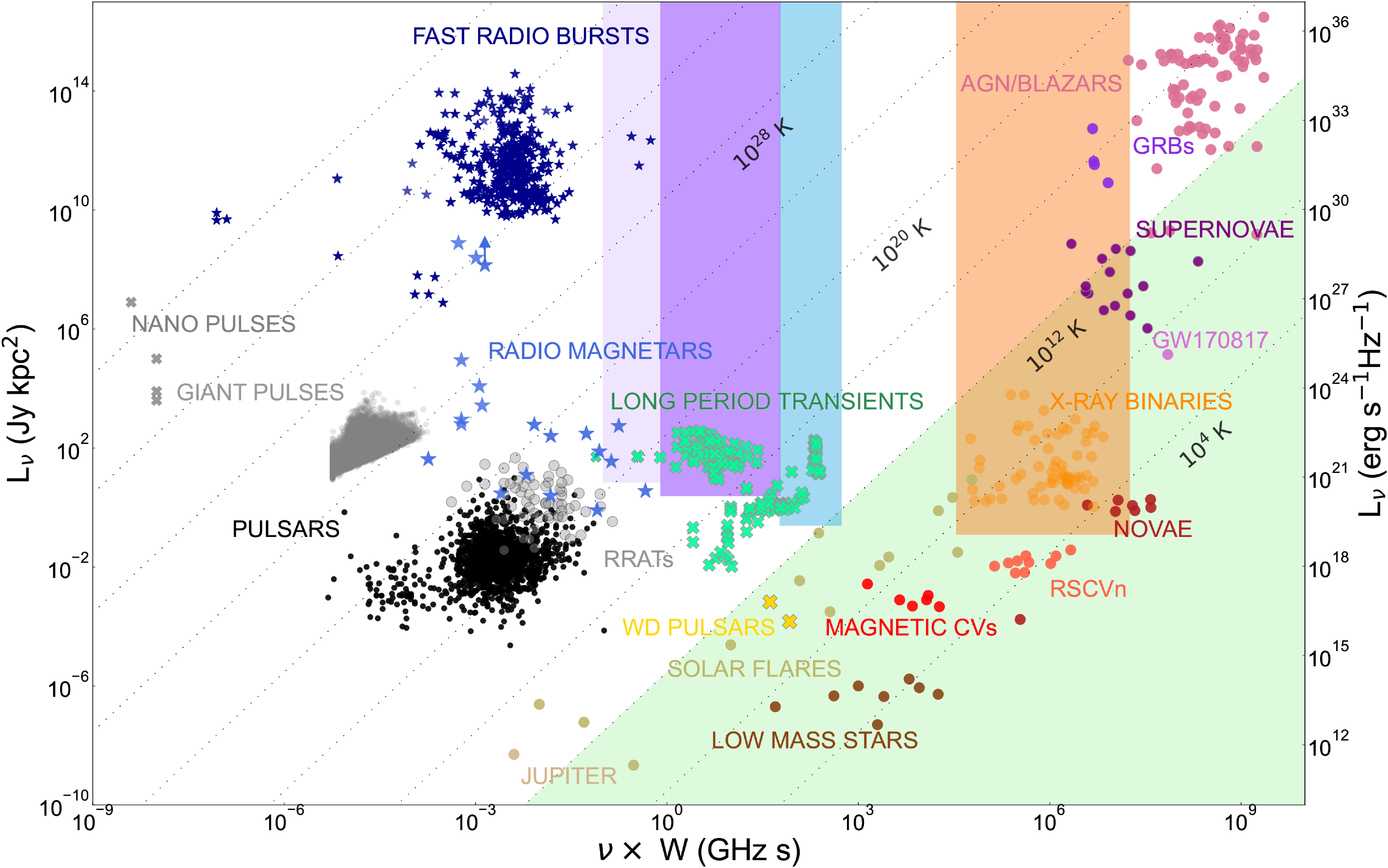
 −

 Ntiles~

 ∘×20∘
 ∼
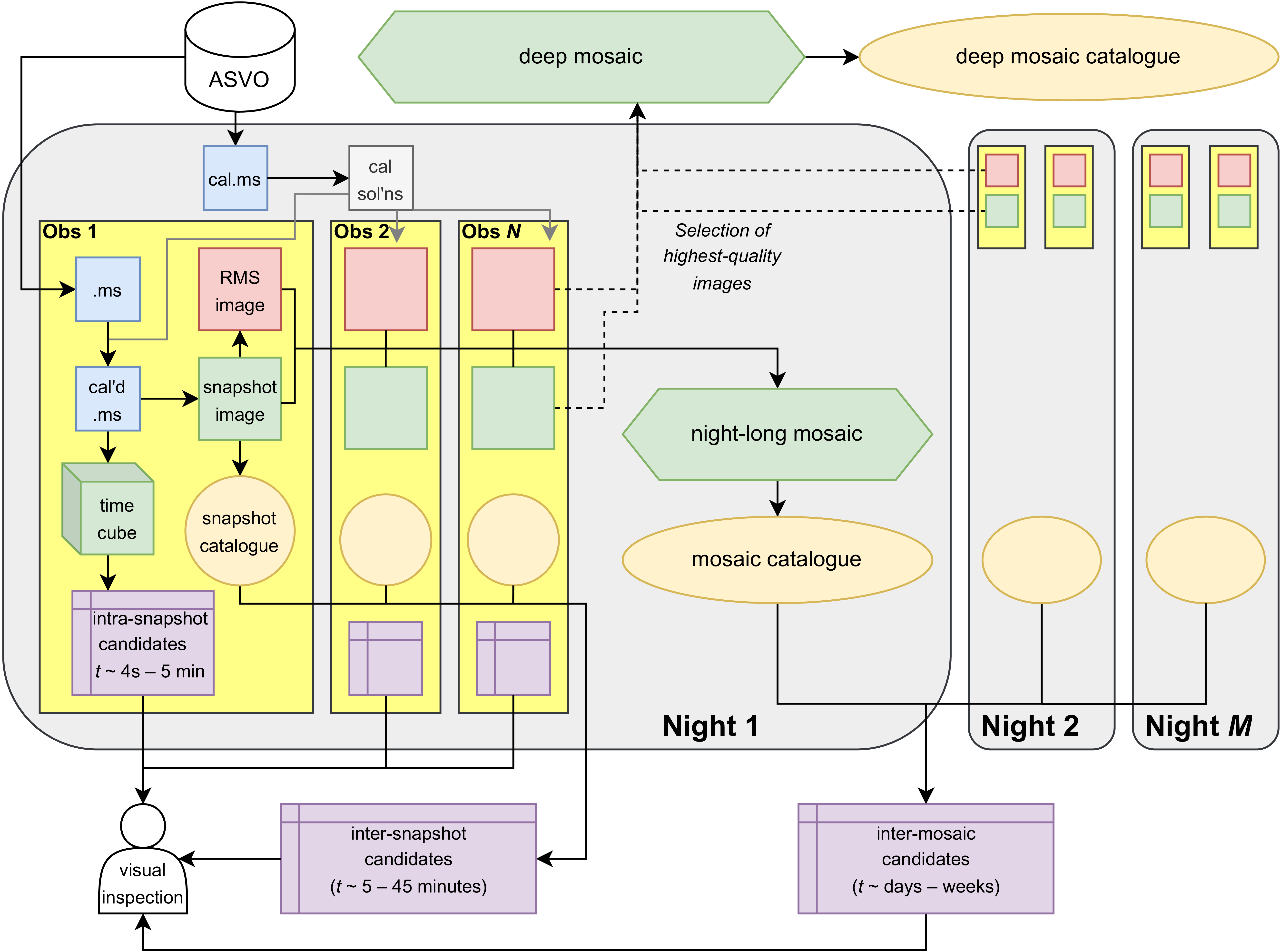
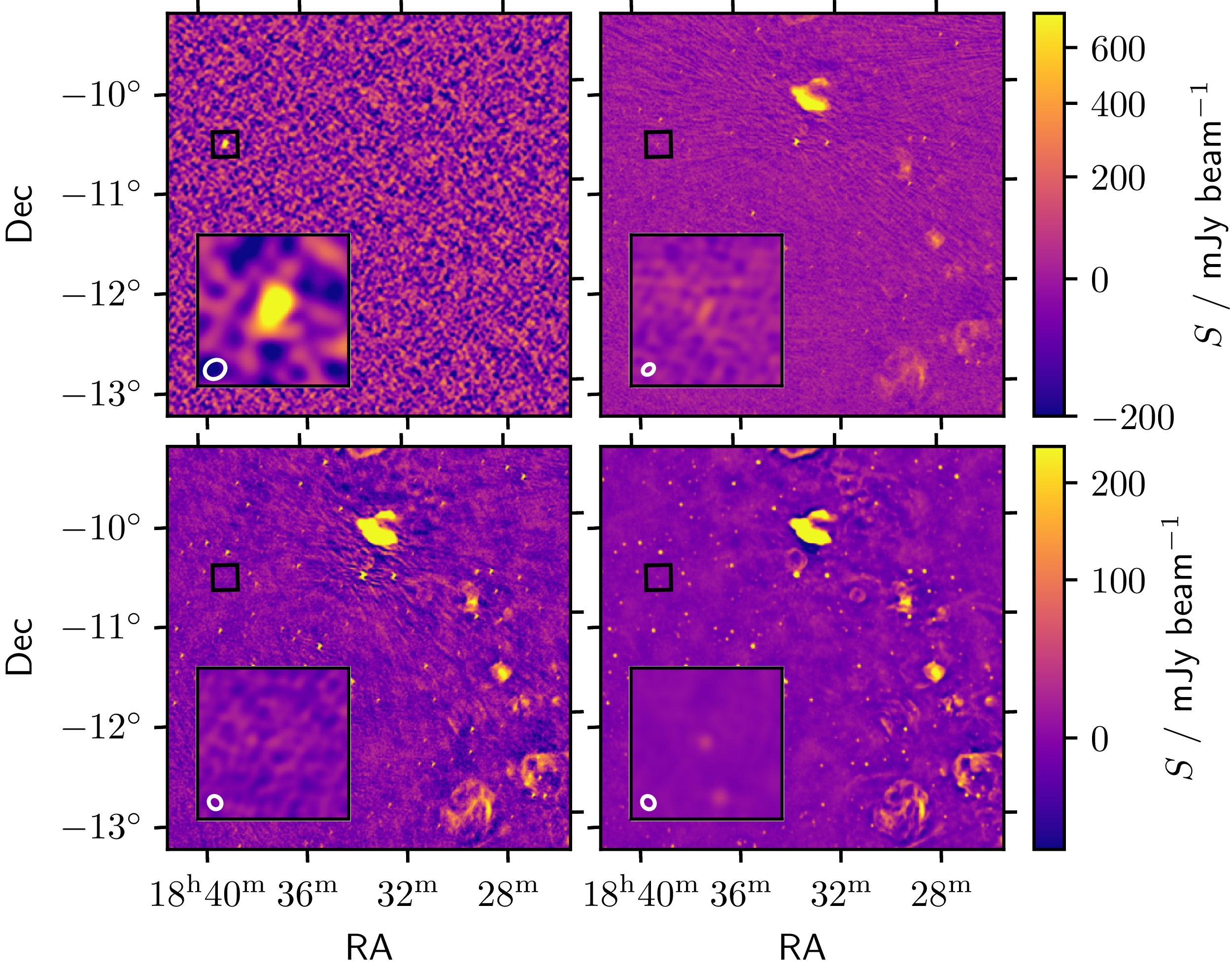
 ∼
 −1
 ∼
 ′
 −
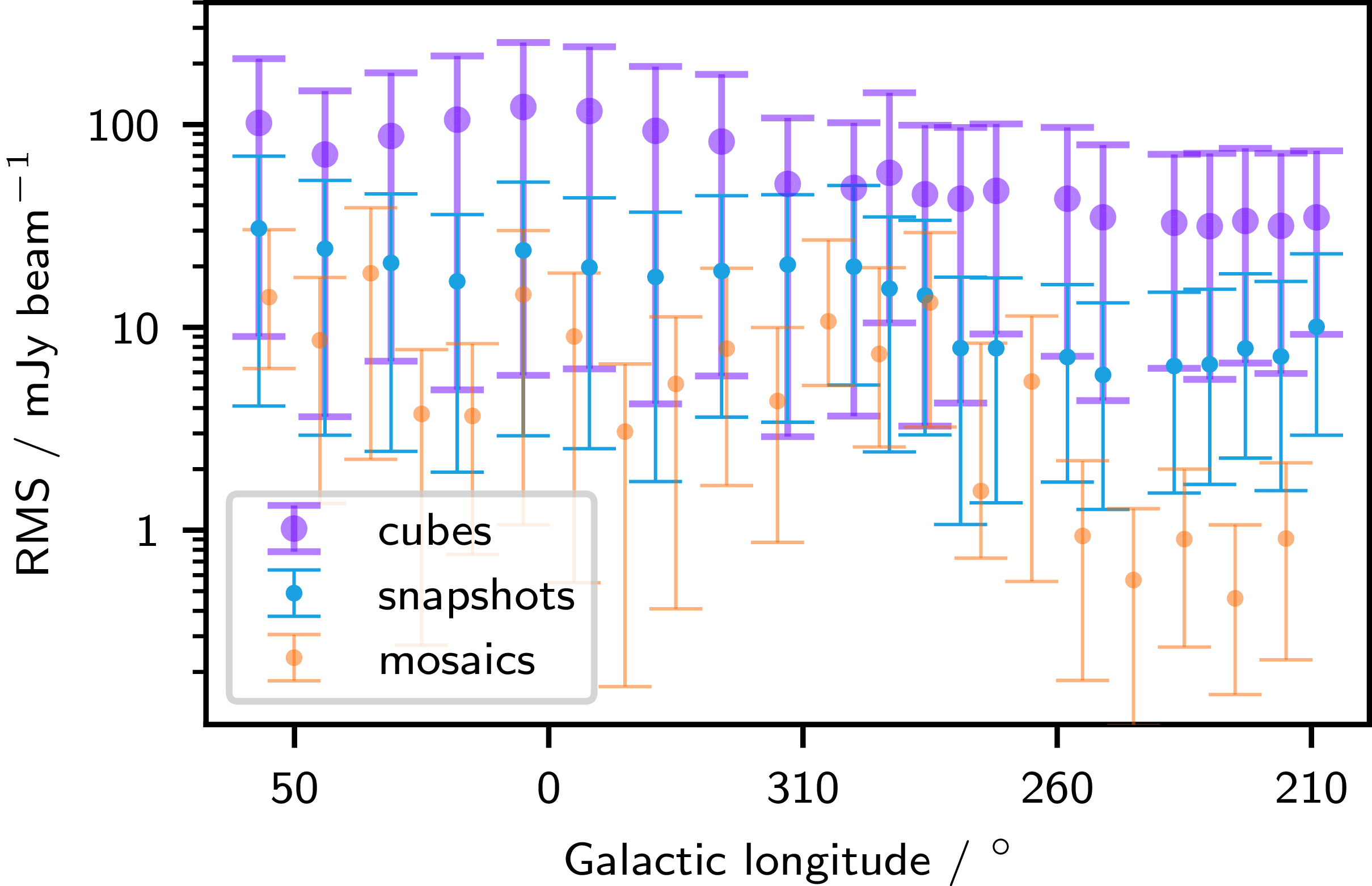
 13∘
 7∘
 l=285∘
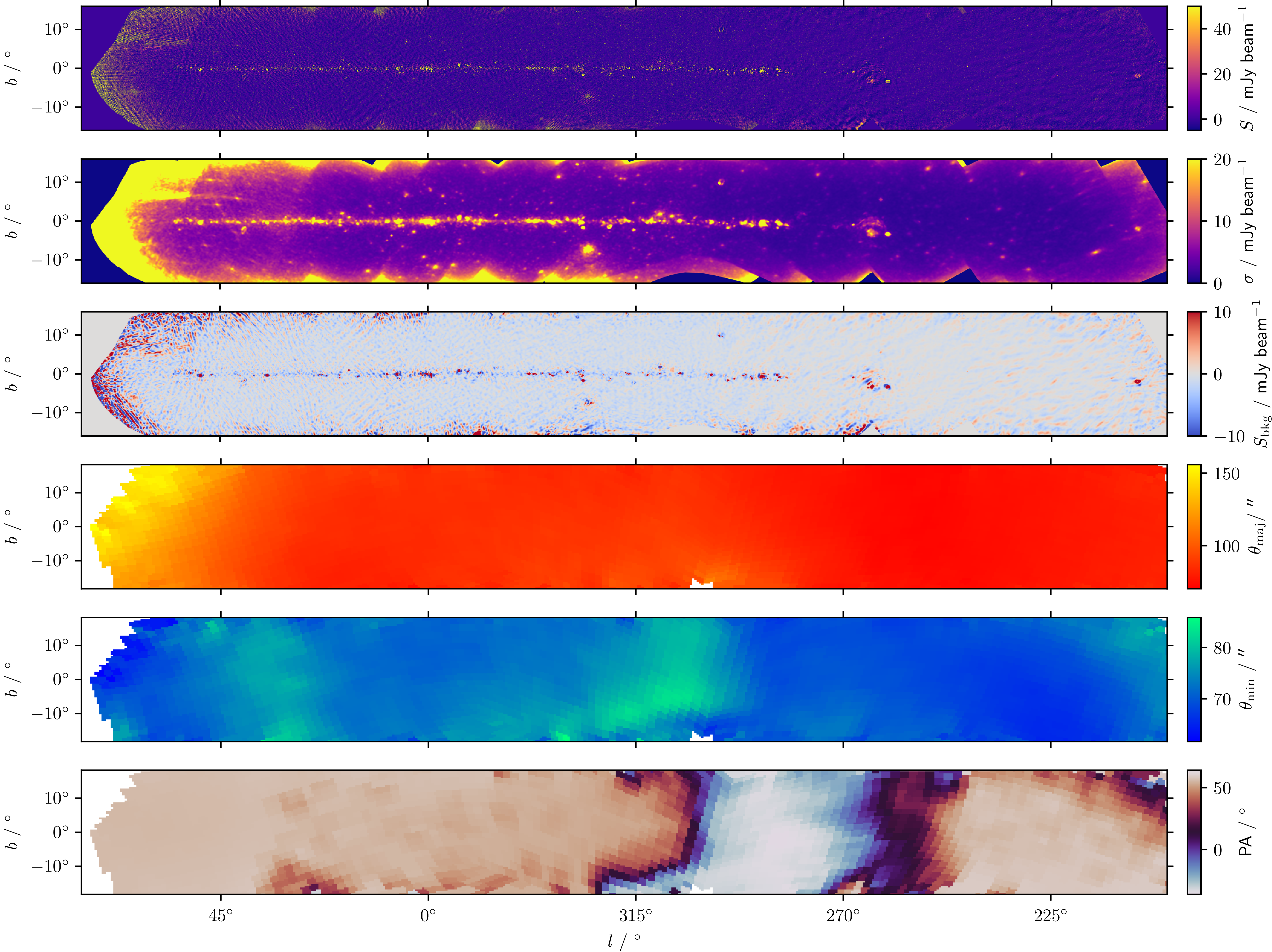
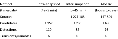
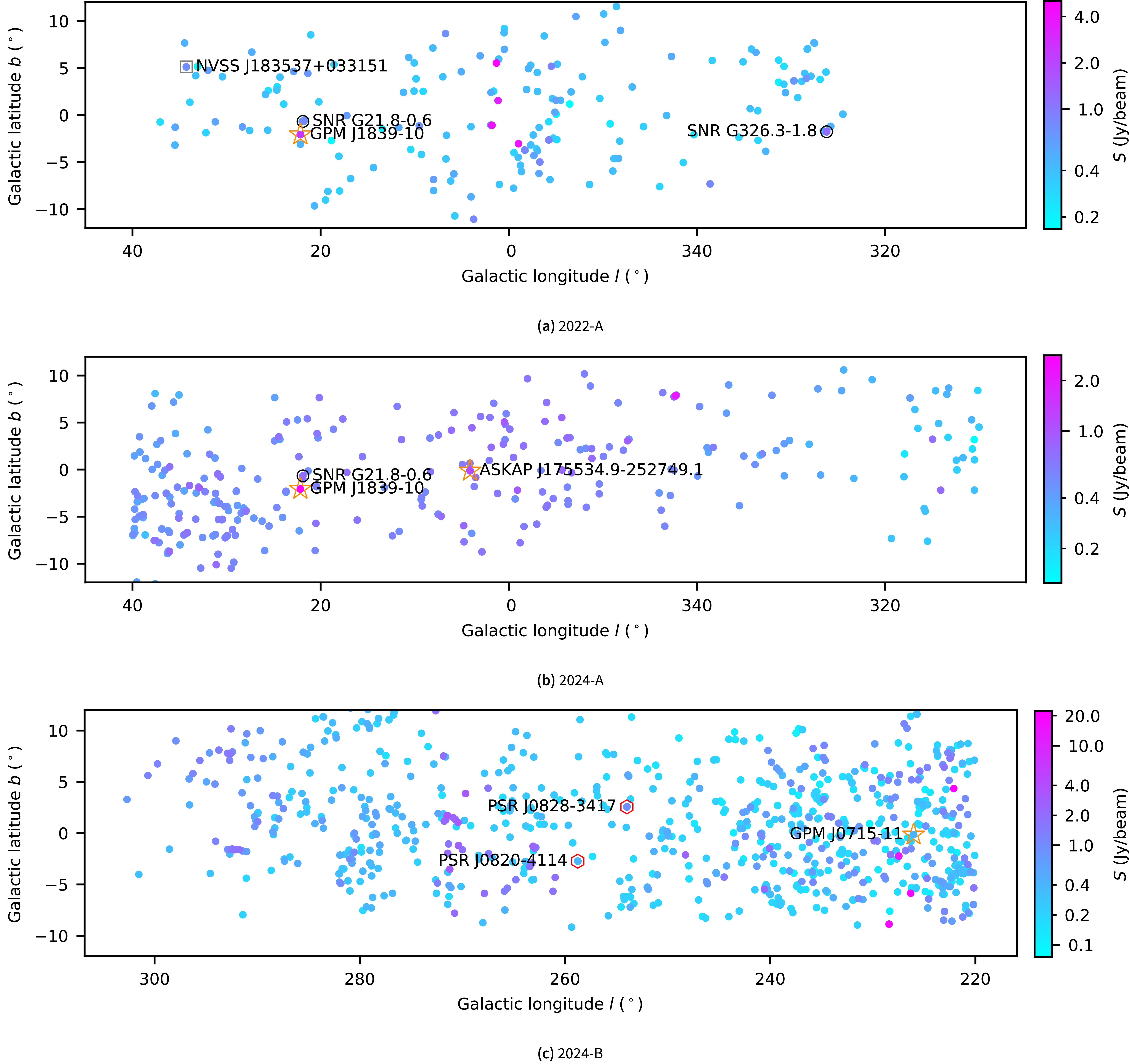
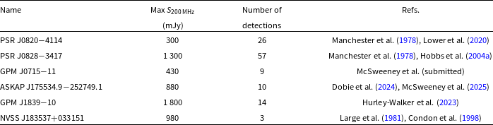
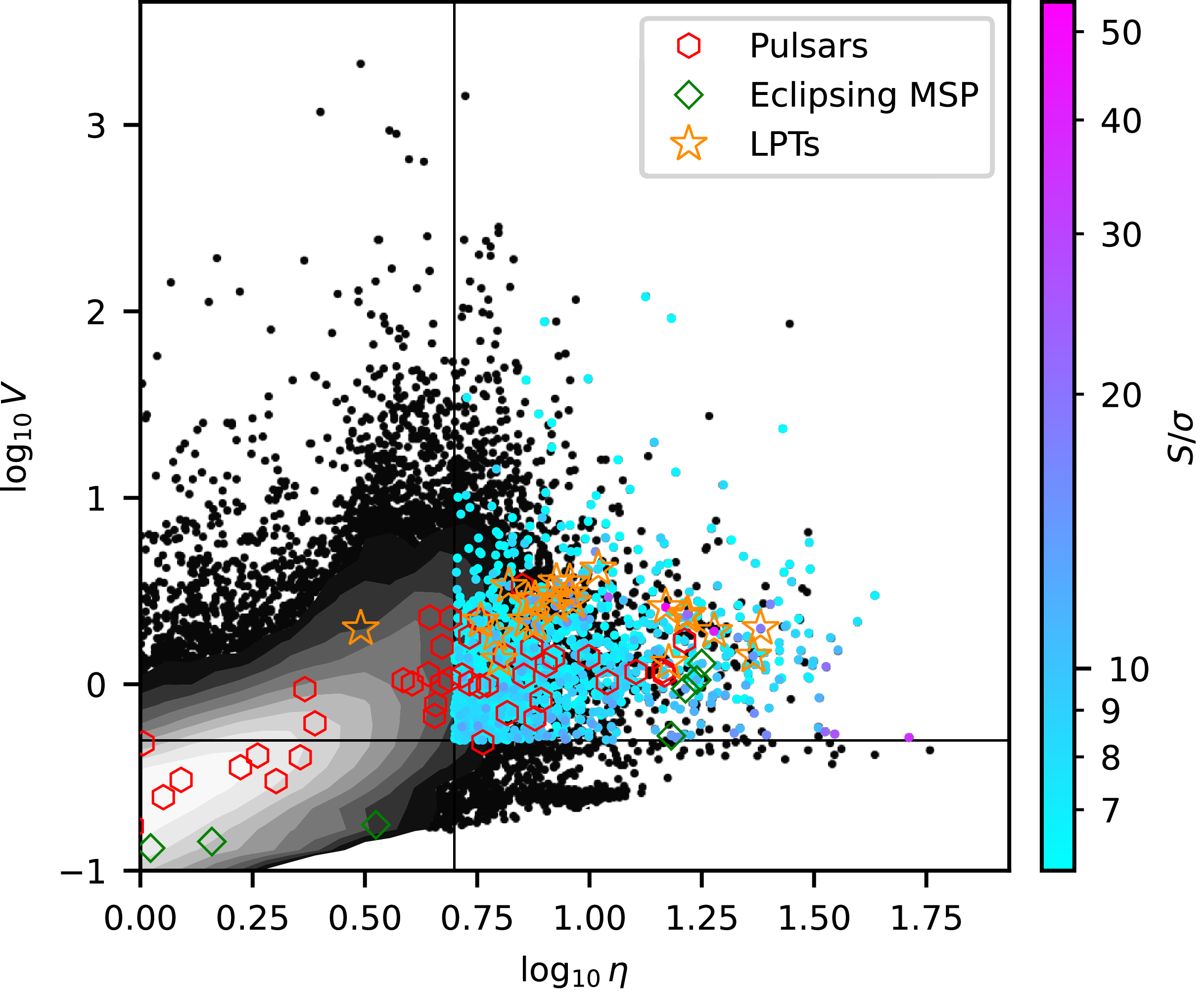
 η
 ∼106
 η>5
 V>0.5
 S/σ>6
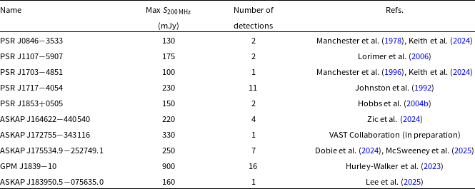
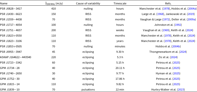
 =Porb
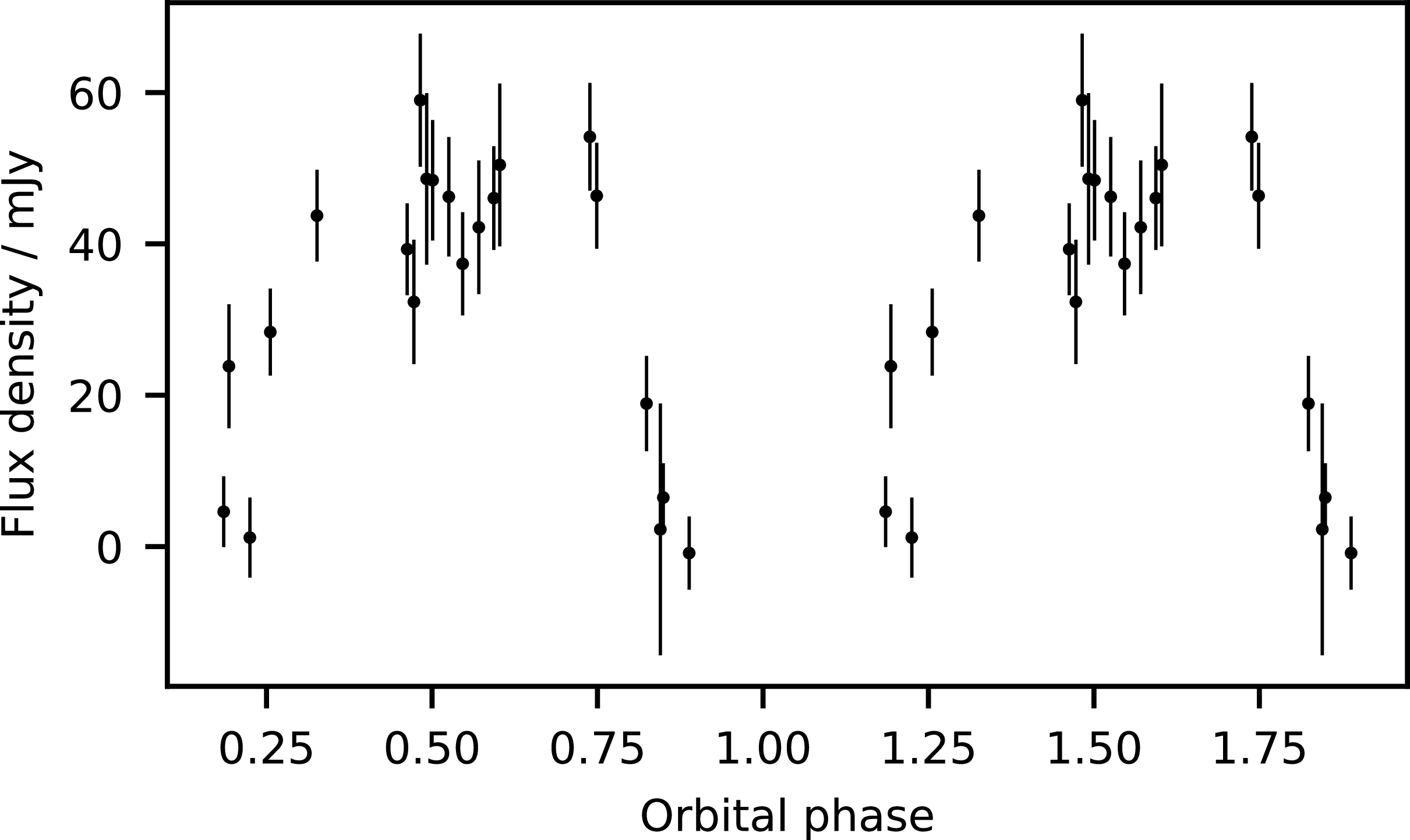
 −
 Porb=0.387339
 Tasc=58097.44433
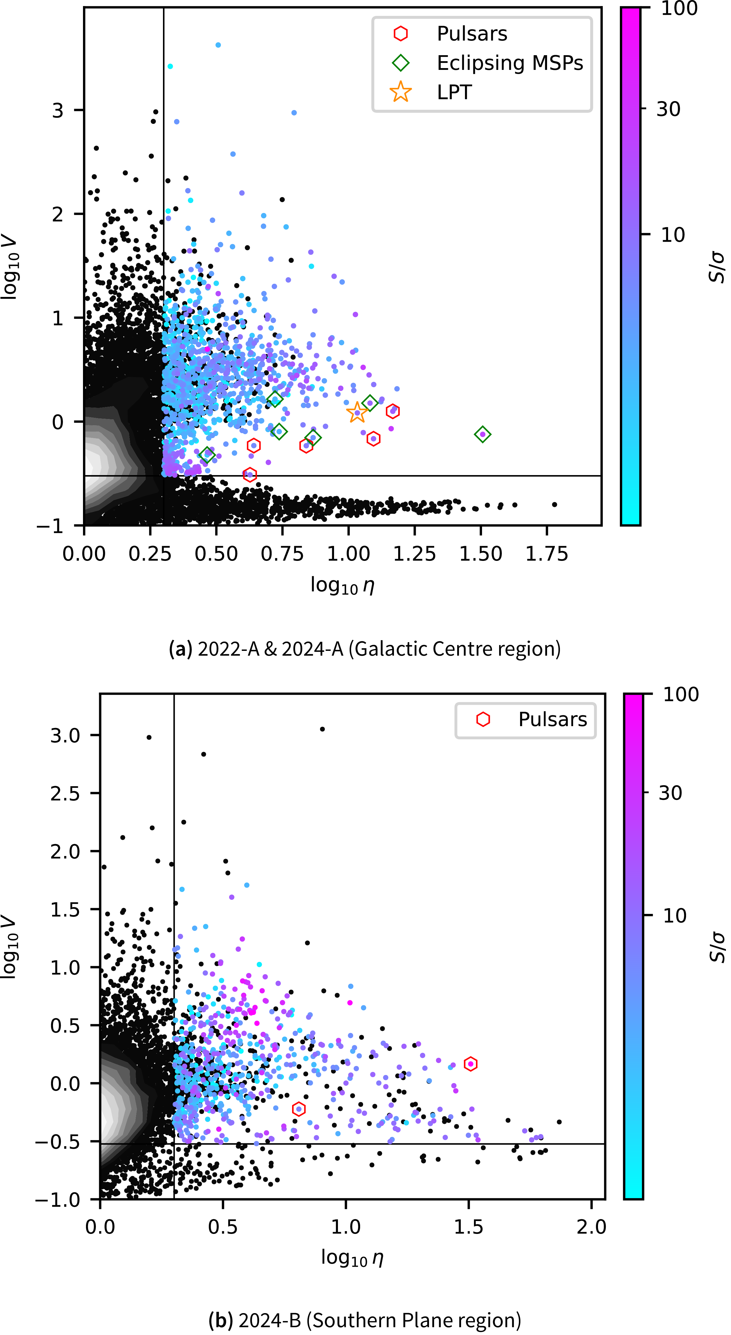
 η
 ∼105
 η>2
 V>0.3
 S/σ>5.5
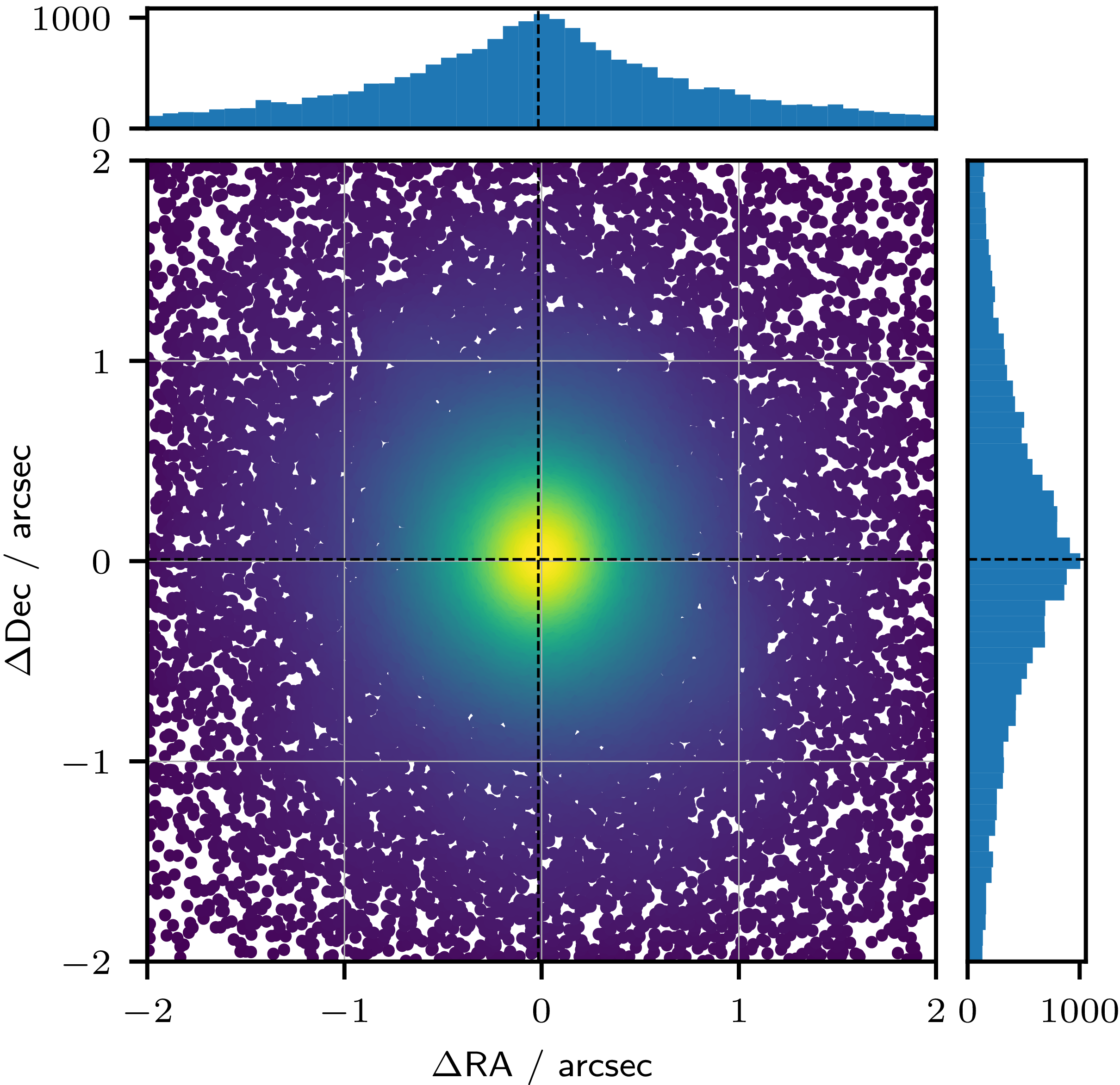
 ΔRA=−17
 ΔDec=9
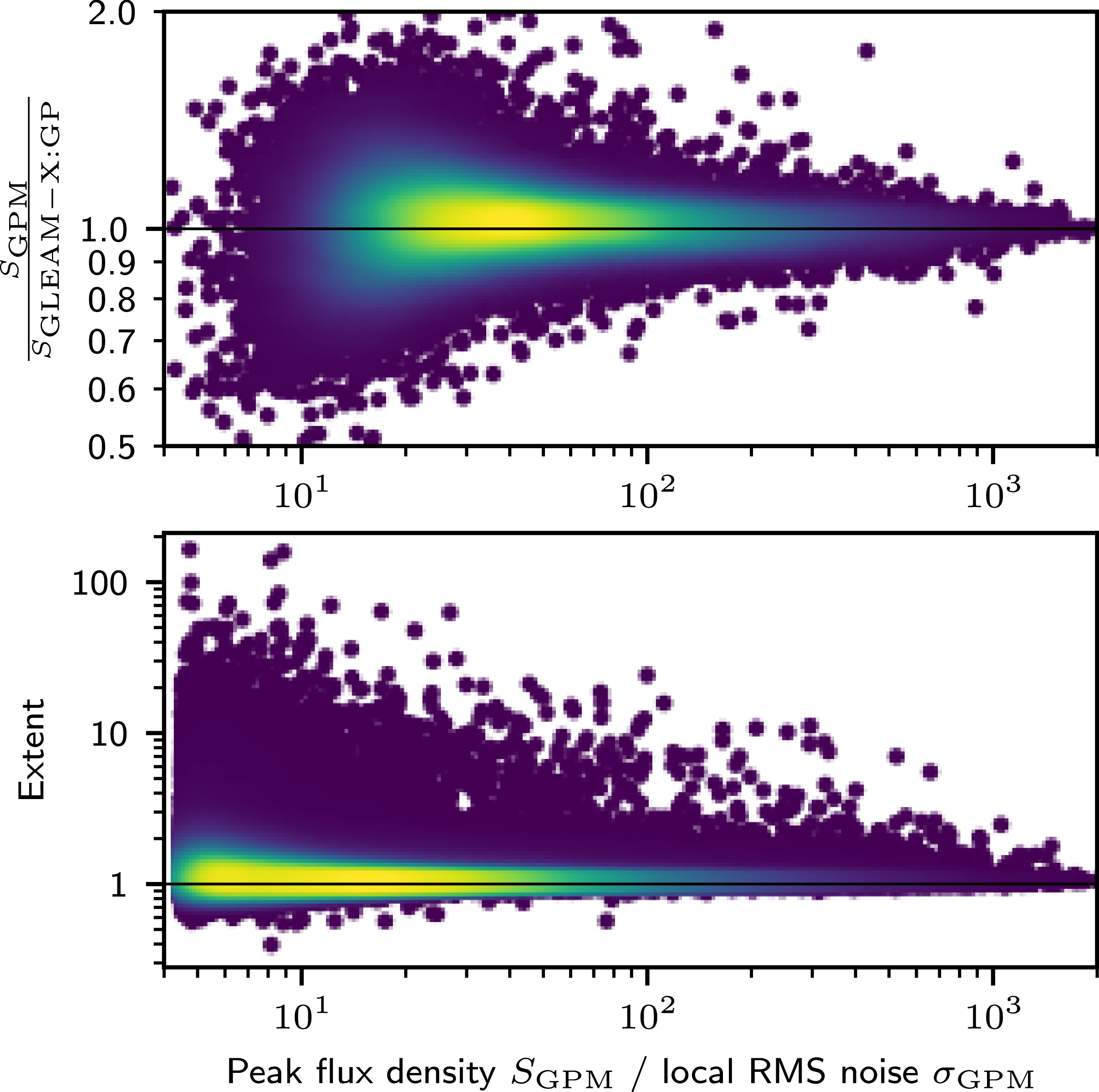
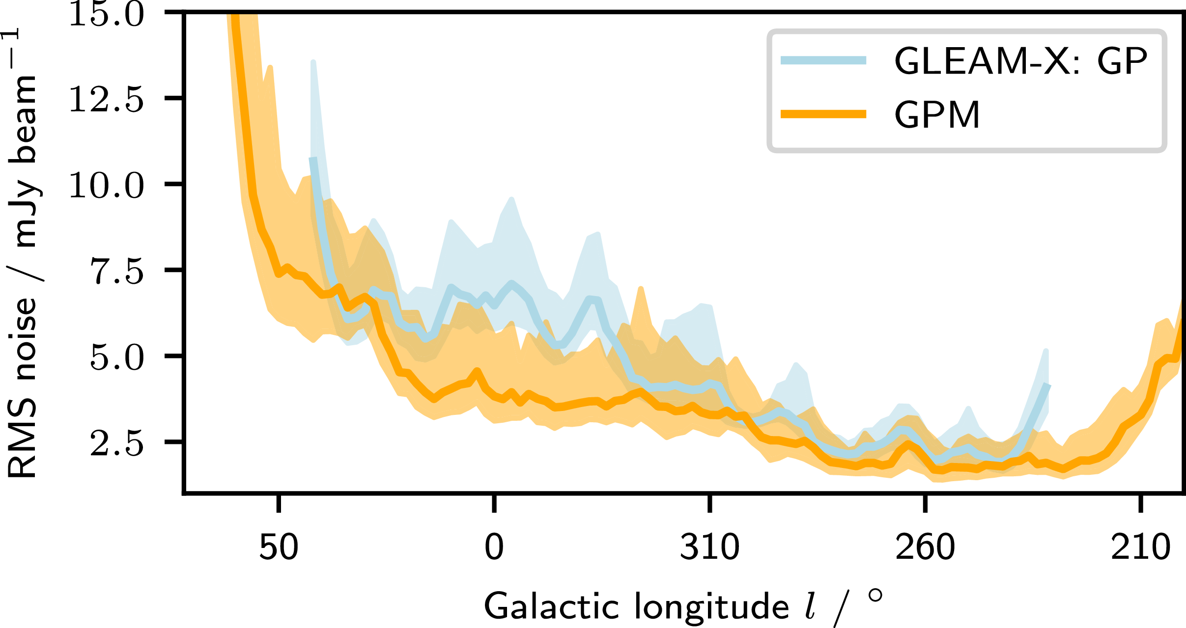
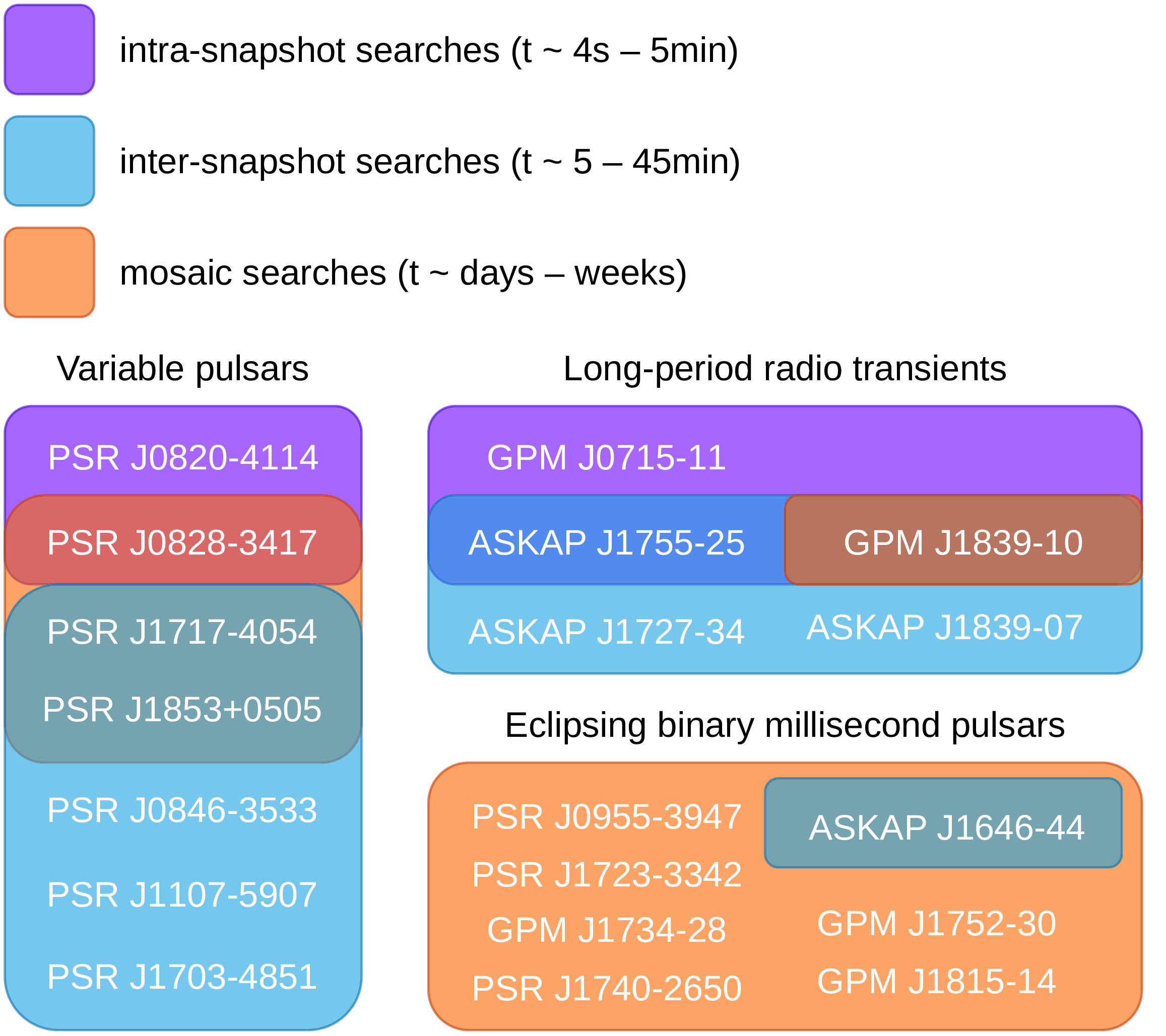
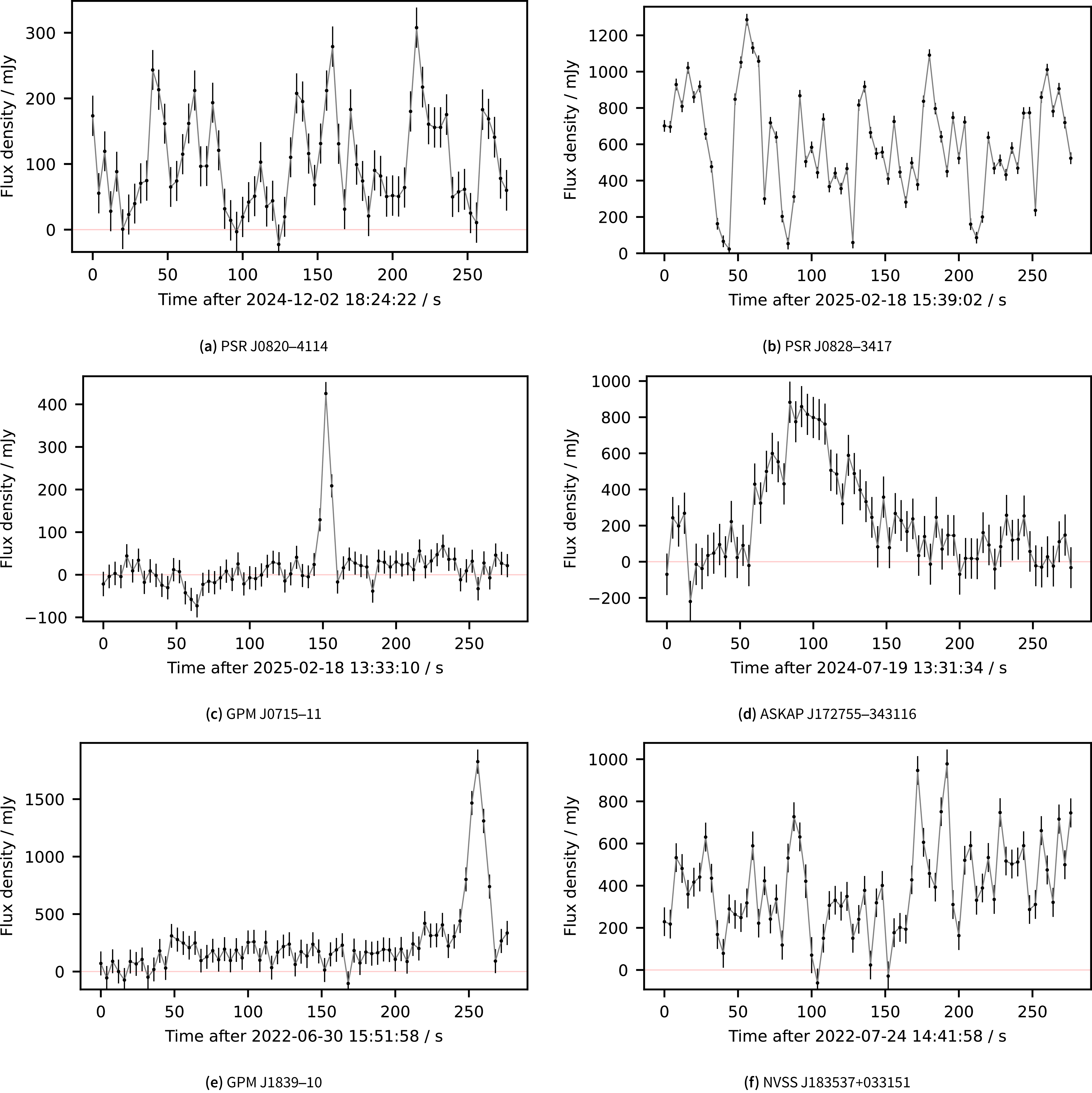
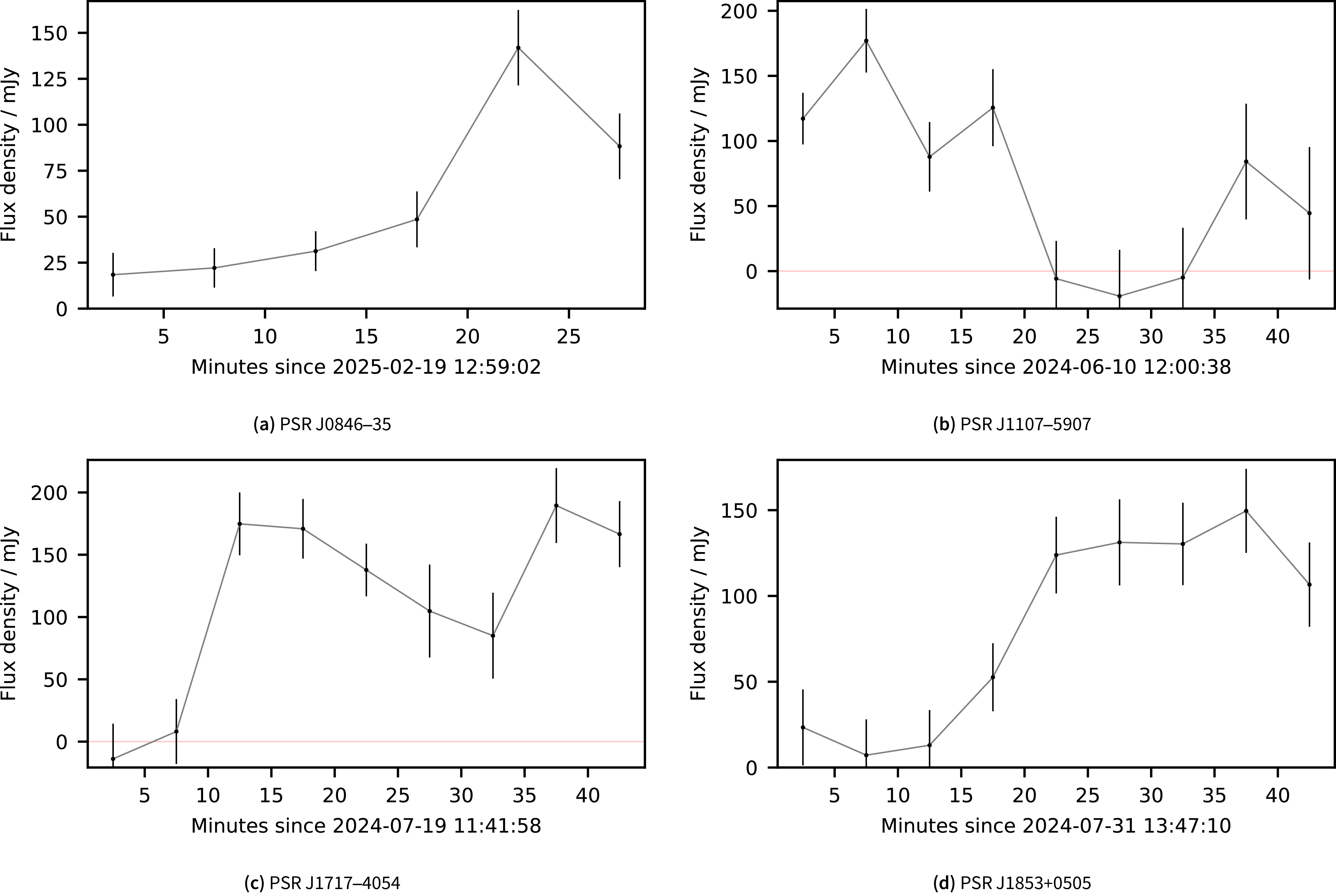
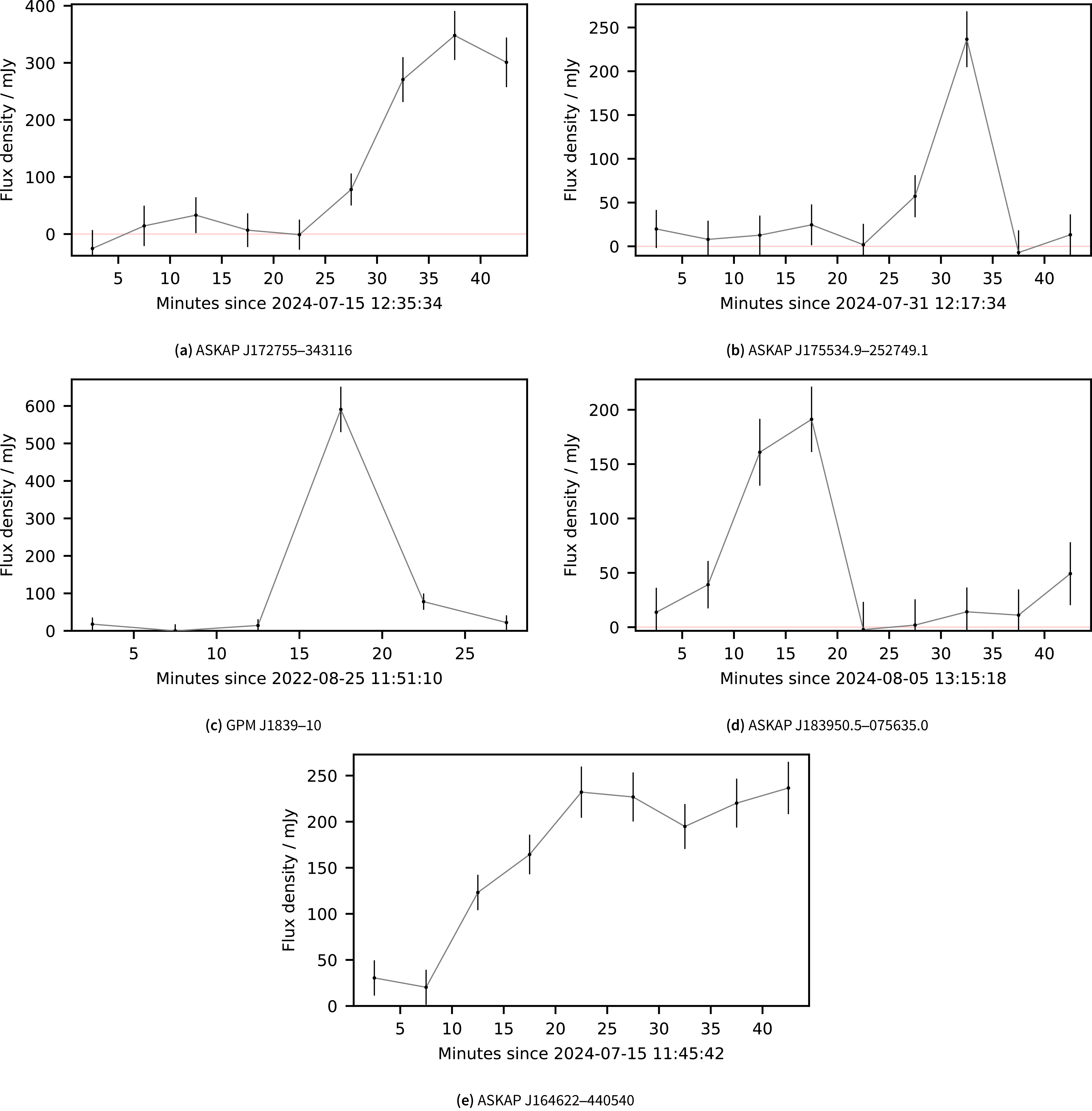
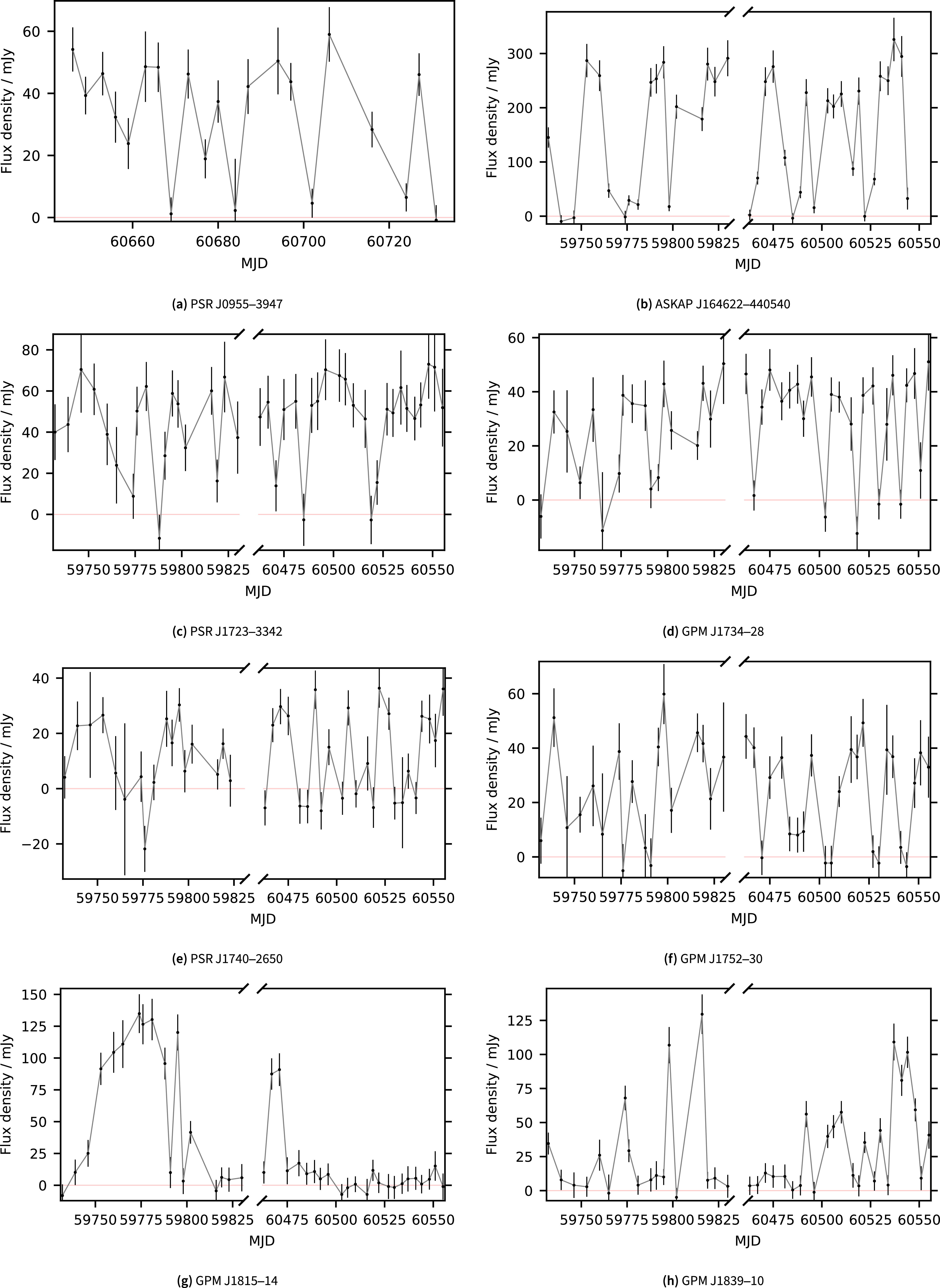
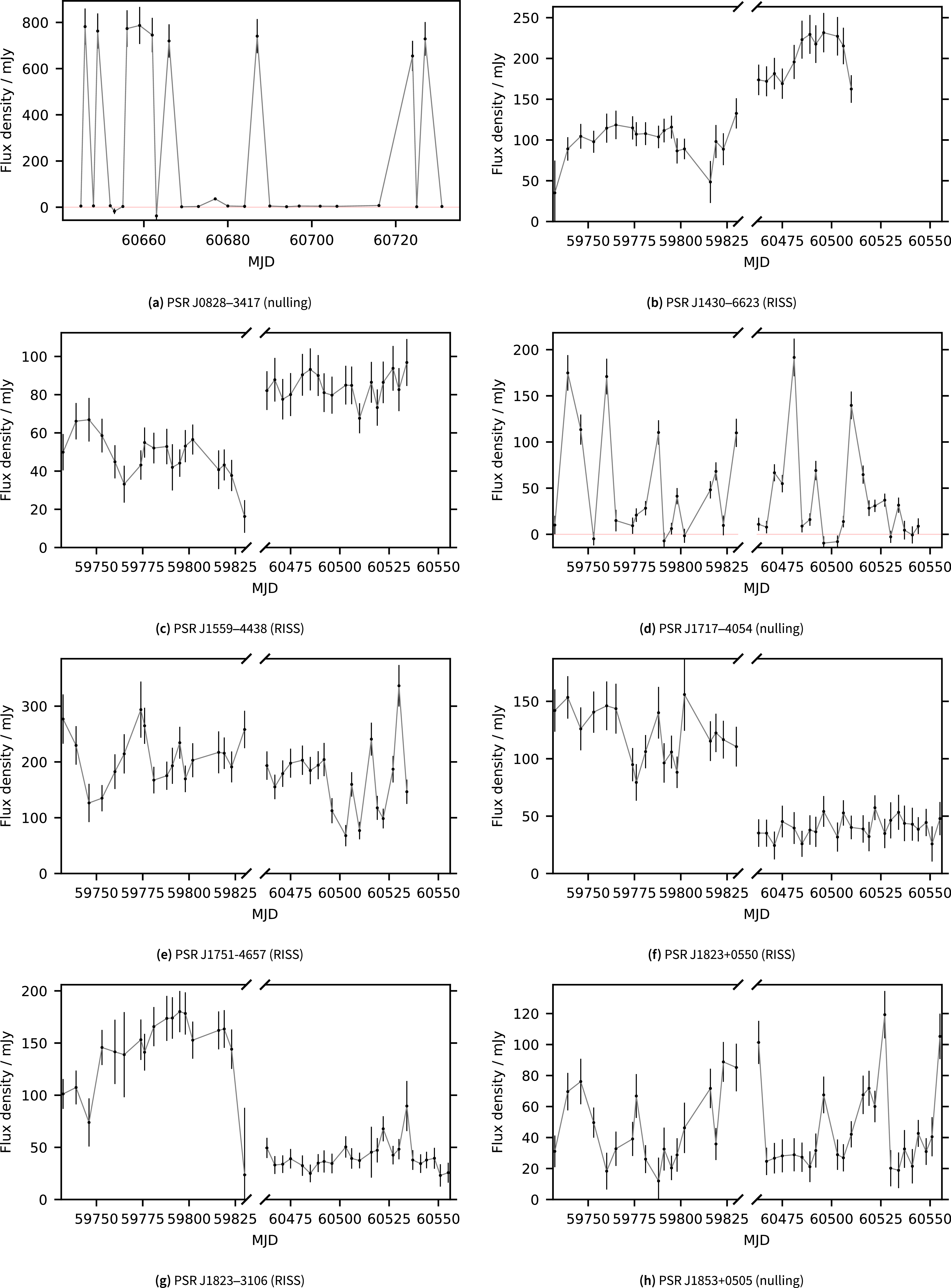
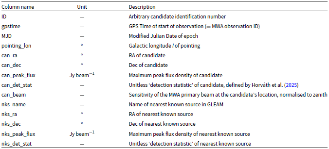
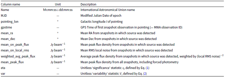
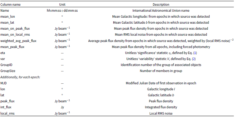
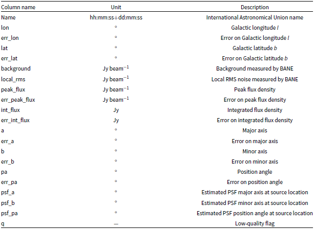

 Open access

