



1 Introduction
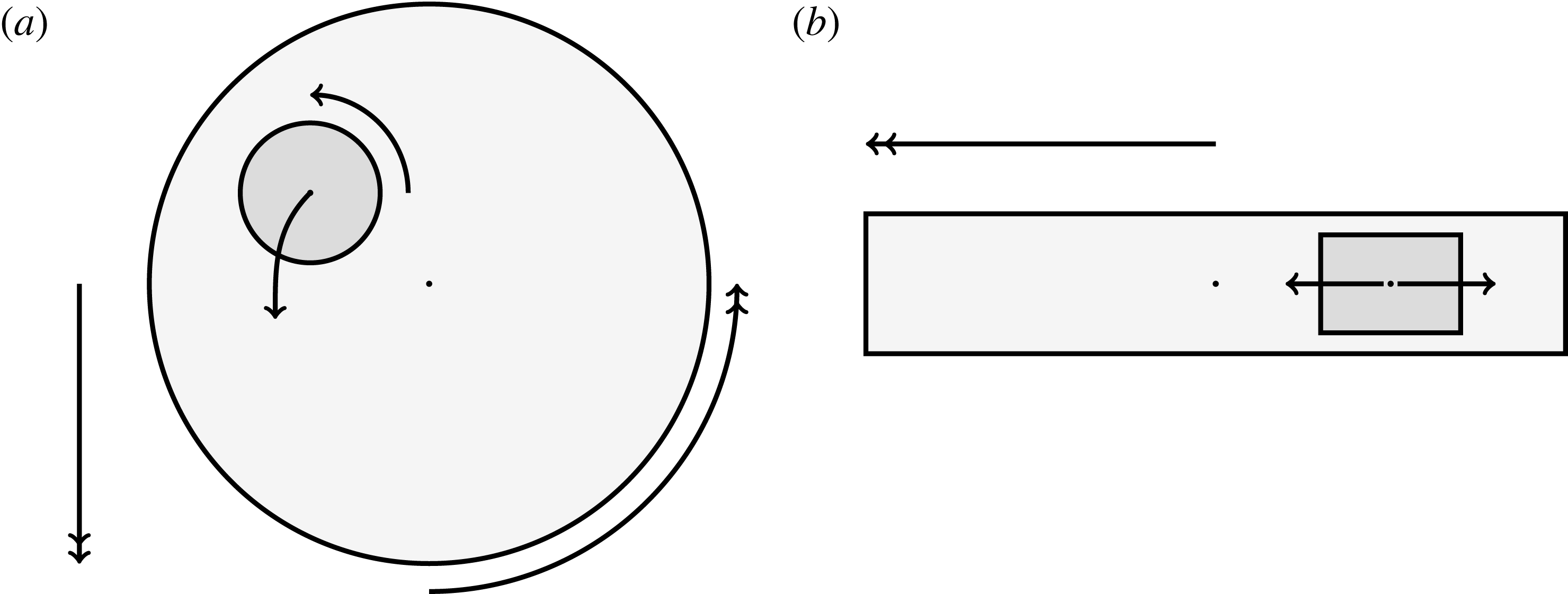
Tissue engineering is a fast-growing interdisciplinary field with the general aim of repairing or replacing damaged body tissue or organs via the engineering of artificial tissues or organs (Lanza, Langer & Vacanti Reference Lanza, Langer and Vacanti2011). One in vitro method to grow tissue involves seeding a rigid porous scaffold with cells – this combination is known as a ‘tissue construct’ or just a ‘construct’– then placing the construct inside a cylindrical petri-dish-shaped bioreactor in which to grow. This high-aspect-ratio vessel (HARV) bioreactor, also known as a rotary cell culture system, is filled with a nutrient-rich fluid, and the cylindrical bioreactor is rotated around its axis at a constant angular velocity, with gravity acting perpendicular to the axis of rotation (figure 1). The consequence of this rotation is the coupled movement of the construct and the fluid, and the motivation behind this is to enhance nutrient delivery to the porous construct via advection, as diffusion alone is not a strong enough transport mechanism to avoid the development of a necrotic core within the growing tissue (Yang et al. Reference Yang, Leong, Du and Chua2001; Khademhosseini, Vacanti & Langer Reference Khademhosseini, Vacanti and Langer2009).
A schematic of the HARV bioreactor set-up in (a) plan view (b) side view. The double-headed arrows denote the forcing in the system, corresponding to gravity (shown in a,b) and rotation of the bioreactor (shown in a). The single-headed arrows denote the movement of the tissue construct, which must be determined as part of the solution.
Tissue growth experiments typically last for weeks within rotating bioreactors (Vunjak-Novakovic et al. Reference Vunjak-Novakovic, Martin, Obradovic, Treppo, Grodzinsky, Langer and Freed1999; Zhang et al. Reference Zhang, Teoh, Chong, Foo, Chng, Choolani and Chan2009). On a short time scale of a few orbits, three different regimes of construct motion are observed experimentally in the HARV bioreactor: steady, settling, and orbital motion (Cummings et al. Reference Cummings, Sawyer, Morgan, Rose and Waters2009). In the steady regime, the construct occupies a stationary position in the bioreactor with respect to the laboratory frame of reference. In the settling regime, the construct undergoes a periodic orbit that does not encircle the bioreactor centre. In the orbital regime, the construct undergoes a periodic orbit that does encircle the bioreactor centre. Experimentally, the steady or settling regimes are preferred, as these are thought to enhance nutrient transfer (Lappa Reference Lappa2003; Cummings et al. Reference Cummings, Sawyer, Morgan, Rose and Waters2009).
More precisely, these three motion regimes appear to be periodic on the short time scale of a few orbits but, in reality, slowly move away from this ‘periodic’ behaviour over hours. Over this time scale, the construct tends to drift in a spiralling motion towards the bioreactor edge. To counteract this drift and maintain the construct in a periodic trajectory it is necessary to vary the angular velocity of the bioreactor over time (Freed & Vunjak-Novakovic Reference Freed and Vunjak-Novakovic1997; Ingram et al. Reference Ingram, Techy, Saroufeem, Yazan, Narayan, Goodwin and Spaulding1997; Gerecht-Nir, Cohen & Itskovitz-Eldor Reference Gerecht-Nir, Cohen and Itskovitz-Eldor2004). In general, this effect has been attributed to the change in density of the construct that occurs via tissue growth on a time scale of hours (Ingram et al. Reference Ingram, Techy, Saroufeem, Yazan, Narayan, Goodwin and Spaulding1997; England, Gorzelak & Trevors Reference England, Gorzelak and Trevors2003; Gerecht-Nir et al. Reference Gerecht-Nir, Cohen and Itskovitz-Eldor2004). We will show that small inertial effects can also give rise to this drift over the same time scale.
Mathematically modelling the full coupled problem of tissue construct movement, fluid flow, and tissue growth within the bioreactor results in a complicated moving-boundary problem. These are notoriously difficult to solve in general, and solutions tend to be computationally expensive (Crank Reference Crank1984). Due to the complexity of these problems, many models of tissue growth in rotating bioreactor systems remove an aspect of the coupling in the moving-boundary problem; either disregarding the tissue movement (Lappa Reference Lappa2003) or the flow problem (Pisu et al. Reference Pisu, Lai, Cincotti, Concas and Cao2004; Nikolaev et al. Reference Nikolaev, Obradovic, Versteeg, Lemon and Williams2010). We present and solve a coupled model for the tissue construct movement and the fluid flow, neglecting tissue growth. Developing an efficient framework for these system characteristics will allow the tissue growth problem to be considered in future work.
There have been some mathematical models that specifically consider the HARV bioreactor and exploit the small aspect ratio to make analytic progress. In Waters et al. (Reference Waters, Cummings, Shakesheff and Rose2006), a cylindrical bioreactor with circular cross-section rotating about its axis is considered for different geometries, including a HARV bioreactor. The tissue construct in this case is modelled by a viscous fluid separated from the external viscous fluid by a membrane. Under this assumption, the linear stability of an initially circular interface between two immiscible fluids within the rotating bioreactor is explored. This paper provides a potential explanation for the irregular nature of some types of tissue grown within such systems. Cummings & Waters (Reference Cummings and Waters2007) extend this work and consider a rotating HARV bioreactor containing a solid impermeable cylindrical tissue construct with circular cross-section. The construct is assumed to sit equidistant between the flat sides of the HARV bioreactor, but is otherwise free to move around the bioreactor according to the forces acting upon it. The authors solve the coupled flow and construct trajectory problem, and their model successfully describes the three different regimes of tissue motion over the short time scale mentioned above. The authors then investigate the nutrient delivery and tissue growth problem for the ‘steady’ case in which the construct is statically suspended within the rotating bioreactor. This paper was followed by Cummings et al. (Reference Cummings, Sawyer, Morgan, Rose and Waters2009), in which the model in Cummings & Waters (Reference Cummings and Waters2007) is extended by introducing one free parameter, and the model predictions are experimentally verified. This free parameter accounts for the relative distances between the construct centre and the flat sides of the bioreactor, and is determined via a fit to experimental data for the construct trajectory.
Whilst significant progress has been made in Waters et al. (Reference Waters, Cummings, Shakesheff and Rose2006), Cummings & Waters (Reference Cummings and Waters2007), Cummings et al. (Reference Cummings, Sawyer, Morgan, Rose and Waters2009), several key features are missing. The tissue construct has previously been modelled as either fully liquid, and separated from the bulk bioreactor flow via a membrane, or fully solid, which means that it has not been possible to consider nutrient delivery to the tissue construct interior. Additionally, in the solid construct cases, the rotation of the construct around its own centre is not considered. This is, in part, due to the shear stress acting on the construct interface being unknown due to the lubrication equations that are used to describe the flow.
The lubrication equations are a good approximation for the flow away from the construct surface in the thin HARV domain. However, the equations break down when the separation of scales in the thin geometry cannot be exploited. This occurs in ‘inner’ regions whose distance from the construct surface is of the same order as the thickness of the bioreactor. In Dalwadi et al. (Reference Dalwadi, Chapman, Waters and Oliver2016), we provide a comprehensive analysis of the flow close to the construct surface. This allows us to systematically derive the correct conditions to couple the ‘outer’ regions where the lubrication equations hold, away from the construct interface, and to determine the shear stress acting on the interface in terms of the outer variables. However, the analysis is restricted to no relative movement between the construct and the bioreactor walls. This must be extended to consider the dynamic problem of a moving construct.
In this paper, we model the coupled flow and construct motion problems of a rotating HARV bioreactor containing a free-moving porous tissue construct with the goals of fully characterizing the flow problem and of exploring the long-time effect of weak inertia on the construct motion. We make significant use of asymptotic techniques to systematically simplify the flow and motion problems that must be solved. We extend the work in Dalwadi et al. (Reference Dalwadi, Chapman, Waters and Oliver2016) to account for the relative movement between the construct and the bioreactor walls; we derive the correct conditions to couple the outer flow in the bioreactor and construct regions, and determine the stress acting on the construct surface. Additionally, we calculate the long-time drift of the construct to determine when the construct will drift out until it hits the bioreactor edge, and when it will tend to a stable limit cycle within the bioreactor.
The question of interfacial conditions on the boundary of a porous obstacle remains an active research area; see, for example, Nield & Bejan (Reference Nield and Bejan2006). We follow Dalwadi et al. (Reference Dalwadi, Chapman, Waters and Oliver2016) and use the interfacial boundary conditions: continuity of flux, continuity of pressure, and no-slip. The first two are derived in Levy & Sanchez-Palencia (Reference Levy and Sanchez-Palencia1975), while the last is a special case of the general tangential slip condition derived in Carraro et al. (Reference Carraro, Goll, Marciniak-Czochra and Mikelić2015).
The structure of the paper is as follows. In § 2, we present and non-dimensionalize a mathematical model for the full flow and trajectory problem. In § 3, we consider a reduced flow problem for a prescribed construct trajectory, with the systematic reduction carried out in appendix A as the analysis closely follows that of Dalwadi et al. (Reference Dalwadi, Chapman, Waters and Oliver2016) with an extension to moving walls. In § 4, we use these flow results to derive closed-form equations of motion for the tissue construct. In § 4.1, we show that the solutions that arise when inertia is neglected can only ever be periodic, and thus cannot account for the experimentally observed construct drift. In § 4.2, we investigate a toy model which captures the important characteristics of the full problem while allowing us to set up the full machinery of the method of multiple scales for a simpler system of similar nonlinear differential equations. In particular, the multiple-scales analysis for this toy problem admits an analytic long-time solution. Once we have fully understood the toy problem, we turn this machinery to the full problem in § 4.3. We find that weak inertia can cause the construct to drift from its periodic orbit, and quantify this effect in a computationally efficient manner. We investigate the bifurcations of the construct trajectory behaviour that arise in the system, and determine for which parameter values a stable limit cycle is possible. Finally, in § 5 we discuss our results and their implications for experimentalists.
2 Model description
We model the fluid culture medium as an incompressible fluid with constant density
 $\unicode[STIX]{x1D70C}$
and constant viscosity
 $\unicode[STIX]{x1D707}$
. The fluid is contained within a HARV bioreactor, which we model as a rotating cylinder of thickness
 $h$
, with a circular cross-section of radius
 $a$
. The tissue construct is modelled as a porous cylinder of thickness
 $d$
and circular cross-section of radius
 $l$
contained within the bioreactor. We show a schematic of the dimensional set-up in figure 2. As the tissue construct is contained within the bioreactor, we have
 $l<a$
and
 $d<h$
. The cylindrical bioreactor rotates with a constant angular velocity of
 $\unicode[STIX]{x1D6FA}$
about its axis, perpendicular to the gravitational force,
 $\boldsymbol{g}$
.
A schematic of the dimensional HARV bioreactor set-up in (a) plan view and (b) side view.
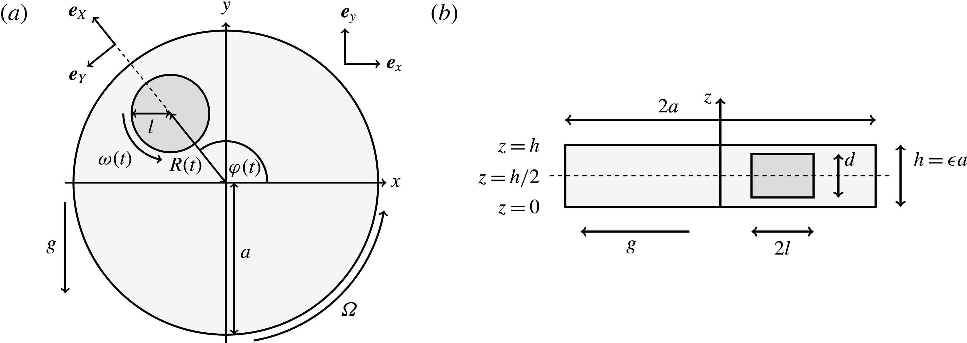
We work in two frames of reference: a stationary laboratory frame, and a frame rotating with the tissue construct centre. We consider the Cartesian coordinate system
 $(x,y,z)$
to be the laboratory frame. This frame is aligned such that gravity acts in the negative
 $y$
-direction. The unit vectors in the positive
 $x$
- and
 $y$
-directions are denoted by
 $\boldsymbol{e}_{x}$
and
 $\boldsymbol{e}_{y}$
respectively, and therefore gravity is given by
 $\boldsymbol{g}=-g\boldsymbol{e}_{y}$
, where
 $g$
is the magnitude of the (constant) gravitational force. The
 $z$
-direction is the longitudinal axis of the bioreactor and has unit vector
 $\boldsymbol{e}_{z}=\boldsymbol{e}_{x}\times \boldsymbol{e}_{y}$
in the positive
 $z$
-direction. The origin of the laboratory frame is located at the bioreactor centre projected onto
 $z=0$
, the lower flat surface of the bioreactor. We define the orthogonal
 $(X,Y)$
frame to have origin at the bioreactor centre, and to rotate with the tissue construct centre. This means that the tissue construct centre can only move along the
 $X$
-axis in this frame. The unit vectors in the positive
 $X$
- and
 $Y$
-directions are denoted by
 $\boldsymbol{e}_{X}$
and
 $\boldsymbol{e}_{Y}$
, respectively. We take
 $(X,Y,z)$
to be the rotating frame.
The movement of the tissue construct centre is assumed to have no component in the
 $\boldsymbol{e}_{z}$
direction, and the gaps between the flat circular sides of the tissue construct and bioreactor are taken to be the same width,
 $(h-d)/2$
. The tissue construct also rotates about its own centre, and we denote this angular velocity by
 $\unicode[STIX]{x1D74E}(t)=\unicode[STIX]{x1D714}(t)\boldsymbol{e}_{z}$
. Hence, we do not allow the construct to wobble around this fixed axis of rotation. These assumptions imply a symmetry in the problem around
 $z=h/2$
. The functions we use to describe the position of the tissue construct centre are:
 $R(t)$
, the distance between the centres of the bioreactor and tissue construct, and
 $\unicode[STIX]{x1D711}(t)$
, the angle that the vector between the bioreactor and tissue construct centres make with the positive
 $x$
-axis. Therefore, in the laboratory frame the velocity of a point within the tissue construct is
 $\boldsymbol{V}_{TC}$
, given by
 $$\begin{eqnarray}\boldsymbol{V}_{TC}=\dot{R}\boldsymbol{e}_{X}+R\dot{\unicode[STIX]{x1D711}}\boldsymbol{e}_{Y}+\unicode[STIX]{x1D74E}\times \boldsymbol{r},\quad \boldsymbol{r}=\boldsymbol{X}-R\boldsymbol{e}_{X},\end{eqnarray}$$
where the first two terms on the right-hand side of (2.1a
) denote the velocity of the tissue construct centre of mass, and the last term denotes the velocity of the construct rotation about its own centre. Here,
 $\boldsymbol{r}$
is the position vector of a point in the tissue construct relative to the tissue construct centre and
 $\boldsymbol{X}$
is the position vector of the same point relative to the bioreactor centre. The functions
 $R(t)$
,
 $\unicode[STIX]{x1D711}(t)$
, and
 $\unicode[STIX]{x1D714}(t)$
are to be determined by considering the net force and torque acting upon the tissue construct.
2.1 Dimensional formulation
2.1.1 Flow equations
We refer to the fluid/flow exterior to the tissue construct as the bulk fluid/flow, and the fluid/flow within the tissue construct as the interior fluid/flow or porous fluid/flow. In the rotating frame, the bulk flow satisfies the incompressible Navier–Stokes equations as follows:
 $$\begin{eqnarray}\displaystyle & \displaystyle \unicode[STIX]{x1D70C}(\dot{\boldsymbol{u}}+(\boldsymbol{u}\boldsymbol{\cdot }\unicode[STIX]{x1D735})\boldsymbol{u}+2\dot{\unicode[STIX]{x1D711}}\boldsymbol{e}_{z}\times \boldsymbol{u}+\ddot{\unicode[STIX]{x1D711}}\boldsymbol{e}_{z}\times \boldsymbol{X}-\dot{\unicode[STIX]{x1D711}}^{2}\boldsymbol{X}^{\bot })=-\unicode[STIX]{x1D735}\tilde{p}+\unicode[STIX]{x1D707}\unicode[STIX]{x1D6FB}^{2}\boldsymbol{u}+\unicode[STIX]{x1D70C}\boldsymbol{g}, & \displaystyle\end{eqnarray}$$
 $$\begin{eqnarray}\displaystyle & \displaystyle \unicode[STIX]{x1D735}\boldsymbol{\cdot }\boldsymbol{u}=0, & \displaystyle\end{eqnarray}$$
 $\boldsymbol{u}=u\boldsymbol{e}_{X}+v\boldsymbol{e}_{Y}+w\boldsymbol{e}_{z}$
is the bulk fluid velocity in the rotating frame,
 $\tilde{p}$
is the bulk fluid pressure,
 $\boldsymbol{X}^{\bot }=X\boldsymbol{e}_{X}+Y\boldsymbol{e}_{Y}$
is the projection of
 $\boldsymbol{X}$
onto the
 $(X,Y)$
plane, and an overdot represents differentiation with respect to time. The interior flow satisfies the incompressible Darcy equations
 $$\begin{eqnarray}\displaystyle & \displaystyle \boldsymbol{Q}-\dot{R}\boldsymbol{e}_{X}+(\dot{\unicode[STIX]{x1D711}}-\unicode[STIX]{x1D714})\boldsymbol{e}_{z}\times \boldsymbol{r}=-{\displaystyle \frac{k}{\unicode[STIX]{x1D707}}}(\unicode[STIX]{x1D735}\tilde{P}-\unicode[STIX]{x1D70C}\boldsymbol{g}), & \displaystyle\end{eqnarray}$$
 $$\begin{eqnarray}\displaystyle & \displaystyle \unicode[STIX]{x1D735}\boldsymbol{\cdot }\boldsymbol{Q}=0, & \displaystyle\end{eqnarray}$$
 $\boldsymbol{Q}=U\boldsymbol{e}_{X}+V\boldsymbol{e}_{Y}+W\boldsymbol{e}_{z}$
is the Darcy flow velocity in the rotating frame,
 $\tilde{P}$
is the interior fluid pressure, and
 $k$
is the permeability of the tissue construct. The transformation of the bulk flow and Darcy velocity from the rotating to the laboratory frame is given by
 $$\begin{eqnarray}\boldsymbol{u}_{LF}=\boldsymbol{u}+\dot{\unicode[STIX]{x1D711}}\boldsymbol{e}_{z}\times \boldsymbol{X},\quad \boldsymbol{Q}_{LF}=\boldsymbol{Q}+\dot{\unicode[STIX]{x1D711}}\boldsymbol{e}_{z}\times \boldsymbol{X},\end{eqnarray}$$
where
 $\boldsymbol{u}_{LF}$
and
 $\boldsymbol{Q}_{LF}$
are the bulk flow and Darcy velocity in the laboratory frame, respectively. Thus, the left-hand side of (2.3a
) is equivalent to
 $\boldsymbol{Q}_{LF}-\boldsymbol{V}_{TC}$
, the difference between the interior flow velocity in the laboratory frame and the velocity of the construct.
We denote the entire bioreactor surface as
 $S$
, and the interface between the tissue construct and the bulk fluid as
 $T$
. On the bioreactor surface, we impose a no-slip condition which, in the rotating frame, is given by
 $$\begin{eqnarray}\boldsymbol{u}=(\unicode[STIX]{x1D6FA}-\dot{\unicode[STIX]{x1D711}})\boldsymbol{e}_{z}\times \boldsymbol{X}\quad \text{on }S.\end{eqnarray}$$
On the tissue construct interface, we impose continuity of normal flux, continuity of pressure, and a no-slip condition (Levy & Sanchez-Palencia Reference Levy and Sanchez-Palencia1975; Carraro et al. Reference Carraro, Goll, Marciniak-Czochra and Mikelić2015) as follows
 $$\begin{eqnarray}\boldsymbol{u}\boldsymbol{\cdot }\boldsymbol{n}=\boldsymbol{Q}\boldsymbol{\cdot }\boldsymbol{n},\quad \tilde{p}=\tilde{P},\quad \boldsymbol{u}\boldsymbol{\cdot }\boldsymbol{s}_{i}=(\dot{R}\boldsymbol{e}_{X}+(\unicode[STIX]{x1D714}-\dot{\unicode[STIX]{x1D711}})\boldsymbol{e}_{z}\times \boldsymbol{r})\boldsymbol{\cdot }\boldsymbol{s}_{i}\quad \text{on }T,\end{eqnarray}$$
where
 $\boldsymbol{n}$
is the unit normal pointing out of the tissue construct and
 $\boldsymbol{s}_{i}$
is any unit tangent vector to the surface.
2.1.2 Construct motion equations
In Dalwadi (Reference Dalwadi2014), the change in the linear and angular momentum of the construct due to the motion of fluid within and across the interface of the construct is found to be negligible when Darcy’s law is applicable, so we disregard these effects in this paper. Then, in the inertial frame, Newton’s second law for linear momentum yields
 $$\begin{eqnarray}\iint _{T}\unicode[STIX]{x1D748}\boldsymbol{\cdot }\boldsymbol{n}\,\text{d}S-M_{c}g(\sin \unicode[STIX]{x1D711}(t)\boldsymbol{e}_{X}+\cos \unicode[STIX]{x1D711}(t)\boldsymbol{e}_{Y})=M_{c}\frac{\text{d}^{2}}{\text{d}t^{2}}(R(t)\boldsymbol{e}_{X}),\end{eqnarray}$$
where
 $\unicode[STIX]{x1D748}$
is the Newtonian stress tensor of the bulk fluid. Here,
 $M_{c}$
is the mass of the wetted construct, equal to the product of the effective construct density
 $\unicode[STIX]{x1D70C}_{c}$
and the construct volume
 $$\begin{eqnarray}M_{c}=\unicode[STIX]{x1D70C}_{c}\unicode[STIX]{x03C0}l^{2}d.\end{eqnarray}$$
In terms of experimentally measurable parameters,
 $\unicode[STIX]{x1D70C}_{c}$
is defined to be
 $$\begin{eqnarray}\unicode[STIX]{x1D70C}_{c}=\unicode[STIX]{x1D70C}\unicode[STIX]{x1D719}+\unicode[STIX]{x1D70C}_{s}(1-\unicode[STIX]{x1D719}),\end{eqnarray}$$
where
 $\unicode[STIX]{x1D719}\in (0,1]$
is the porosity of the construct and
 $\unicode[STIX]{x1D70C}_{s}$
is the density of the solid matrix within the construct. We note that
 $\unicode[STIX]{x1D719}=0$
for a solid construct and
 $\unicode[STIX]{x1D719}=1$
for a fully fluid construct, but that the coupling conditions we derive in appendix A at first order are not valid for the lower limit. The first term on the left-hand side of (2.7) is the hydrodynamical force on the construct surface (and also contains the buoyancy forces), the second term on the left-hand side is the weight of the wet mass of the construct, and the right-hand side is the rate of change of linear momentum.
Similarly, Newton’s second law for angular momentum implies that
 $$\begin{eqnarray}\iint _{T}\boldsymbol{r}\times (\unicode[STIX]{x1D748}\boldsymbol{\cdot }\boldsymbol{n})\,\text{d}S={\displaystyle \frac{M_{c}l^{2}}{2}}\frac{\text{d}\unicode[STIX]{x1D714}}{\text{d}t}\boldsymbol{e}_{z},\end{eqnarray}$$
where the left-hand side is the hydrodynamical torque on the construct surface, and the right-hand side is the rate of change of angular momentum.
2.2 Dimensionless equations
We non-dimensionalize by setting
 $$\begin{eqnarray}\left.\begin{array}{@{}c@{}}(X,Y,z)=a(X^{\ast },Y^{\ast },\unicode[STIX]{x1D716}z^{\ast }),\quad (l,R)=a(b^{\ast },R^{\ast }),\\ t=\unicode[STIX]{x1D6FA}^{-1}t^{\ast },\quad \unicode[STIX]{x1D714}=\unicode[STIX]{x1D6FA}\unicode[STIX]{x1D714}^{\ast },\\ (u,v,w)=a\unicode[STIX]{x1D6FA}(u^{\ast },v^{\ast },\unicode[STIX]{x1D716}w^{\ast }),\quad (U,V,W)=a\unicode[STIX]{x1D6FA}(U^{\ast },V^{\ast },\unicode[STIX]{x1D716}W^{\ast }),\\ (\tilde{p},\tilde{P})=\unicode[STIX]{x1D707}\unicode[STIX]{x1D6FA}\unicode[STIX]{x1D716}^{-2}(\tilde{p}^{\ast },\tilde{P}^{\ast }),\quad \unicode[STIX]{x1D748}=\unicode[STIX]{x1D707}\unicode[STIX]{x1D6FA}\unicode[STIX]{x1D716}^{-2}\unicode[STIX]{x1D748}^{\ast },\end{array}\right\}\end{eqnarray}$$
where
 $\unicode[STIX]{x1D716}=h/a$
. In (2.11), asterisks denote dimensionless variables, and we henceforth drop asterisks for convenience. In dimensionless variables, we continue to use the vector notations
 $\boldsymbol{X}=X\boldsymbol{e}_{X}+Y\boldsymbol{e}_{Y}+z\boldsymbol{e}_{z}$
,
 $\boldsymbol{r}=\boldsymbol{X}-R\boldsymbol{e}_{X}$
,
 $\boldsymbol{u}=u\boldsymbol{e}_{X}+v\boldsymbol{e}_{Y}+w\boldsymbol{e}_{z}$
and
 $\boldsymbol{Q}=U\boldsymbol{e}_{X}+V\boldsymbol{e}_{Y}+W\boldsymbol{e}_{z}$
. The bulk flow equations (2.2) become
 $$\begin{eqnarray}\displaystyle & \displaystyle \unicode[STIX]{x1D716}Re(\dot{u}+(\boldsymbol{u}\boldsymbol{\cdot }\unicode[STIX]{x1D735})u-2\dot{\unicode[STIX]{x1D711}}v-\ddot{\unicode[STIX]{x1D711}}Y-\dot{\unicode[STIX]{x1D711}}^{2}X)=-p_{X}+\unicode[STIX]{x1D716}^{2}\unicode[STIX]{x1D6FB}_{\bot }^{2}u+u_{zz}, & \displaystyle\end{eqnarray}$$
 $$\begin{eqnarray}\displaystyle & \displaystyle \unicode[STIX]{x1D716}Re(\dot{v}+(\boldsymbol{u}\boldsymbol{\cdot }\unicode[STIX]{x1D735})v+2\dot{\unicode[STIX]{x1D711}}u+\ddot{\unicode[STIX]{x1D711}}X-\dot{\unicode[STIX]{x1D711}}^{2}Y)=-p_{Y}+\unicode[STIX]{x1D716}^{2}\unicode[STIX]{x1D6FB}_{\bot }^{2}v+v_{zz}, & \displaystyle\end{eqnarray}$$
 $$\begin{eqnarray}\displaystyle & \displaystyle \unicode[STIX]{x1D716}^{3}Re({\dot{w}}+(\boldsymbol{u}\boldsymbol{\cdot }\unicode[STIX]{x1D735})w)=-p_{z}+\unicode[STIX]{x1D716}^{4}\unicode[STIX]{x1D6FB}_{\bot }^{2}w+\unicode[STIX]{x1D716}^{2}w_{zz}, & \displaystyle\end{eqnarray}$$
 $$\begin{eqnarray}\displaystyle & \displaystyle \unicode[STIX]{x1D735}\boldsymbol{\cdot }\boldsymbol{u}=0, & \displaystyle\end{eqnarray}$$
 $\unicode[STIX]{x1D6FB}_{\bot }^{2}=\unicode[STIX]{x2202}_{XX}+\unicode[STIX]{x2202}_{YY}$
, and the Reynolds number
 $Re=\unicode[STIX]{x1D70C}h(a\unicode[STIX]{x1D6FA})/\unicode[STIX]{x1D707}$
. We emphasize that the length scale in the Reynolds number adopted here is the bioreactor thickness and not its radius. The reduced pressure is given by
 $p=\tilde{p}+B(X\sin \unicode[STIX]{x1D711}+Y\cos \unicode[STIX]{x1D711})$
, where the Bond number, a measure of the gravitational strength compared to viscous effects, is
 $B=\unicode[STIX]{x1D716}^{2}\unicode[STIX]{x1D70C}ag/(\unicode[STIX]{x1D707}\unicode[STIX]{x1D6FA})$
.
The interior flow equations (2.3) become
 $$\begin{eqnarray}\displaystyle & \displaystyle U-\dot{R}-(\dot{\unicode[STIX]{x1D711}}-\unicode[STIX]{x1D714})Y=-KP_{X}, & \displaystyle\end{eqnarray}$$
 $$\begin{eqnarray}\displaystyle & \displaystyle V+(\dot{\unicode[STIX]{x1D711}}-\unicode[STIX]{x1D714})(X-R)=-KP_{Y}, & \displaystyle\end{eqnarray}$$
 $$\begin{eqnarray}\displaystyle & \displaystyle \unicode[STIX]{x1D716}^{2}W=-KP_{z}, & \displaystyle\end{eqnarray}$$
 $$\begin{eqnarray}\displaystyle & \displaystyle \unicode[STIX]{x1D735}\boldsymbol{\cdot }\boldsymbol{Q}=0, & \displaystyle\end{eqnarray}$$
 $K=k/(\unicode[STIX]{x1D716}a)^{2}$
is the Darcy number, and the reduced pressure is given by
 $P=\tilde{P}+B(X\sin \unicode[STIX]{x1D711}+Y\cos \unicode[STIX]{x1D711})$
.
On the bioreactor boundary
 $S$
, the no-slip boundary condition (2.5) becomes
 $$\begin{eqnarray}\boldsymbol{u}=(1-\dot{\unicode[STIX]{x1D711}})\boldsymbol{e}_{z}\times \boldsymbol{X}\quad \text{on }S.\end{eqnarray}$$
On the tissue construct interface, the boundary conditions (2.6) become
 $$\begin{eqnarray}\boldsymbol{u}\boldsymbol{\cdot }\boldsymbol{n}=\boldsymbol{Q}\boldsymbol{\cdot }\boldsymbol{n},\quad p=P,\quad \boldsymbol{u}\boldsymbol{\cdot }\boldsymbol{s}_{i}=(\dot{R}\boldsymbol{e}_{X}+(\unicode[STIX]{x1D714}-\dot{\unicode[STIX]{x1D711}})\boldsymbol{e}_{z}\times \boldsymbol{r})\boldsymbol{\cdot }\boldsymbol{s}_{i}\quad \text{on }T.\end{eqnarray}$$
Finally, we give the dimensionless form of the construct motion (2.7) and (2.10), which become
 $$\begin{eqnarray}\displaystyle & \displaystyle \boldsymbol{f}_{c}+\boldsymbol{f}_{f}+\boldsymbol{f}_{g}=\unicode[STIX]{x1D716}^{2}Re\bar{\unicode[STIX]{x1D70C}}{\mathcal{V}}\frac{\text{d}^{2}}{\text{d}t^{2}}(R(t)\boldsymbol{e}_{X}), & \displaystyle\end{eqnarray}$$
 $$\begin{eqnarray}\displaystyle & \displaystyle \unicode[STIX]{x1D749}_{c}+\unicode[STIX]{x1D749}_{f}=\unicode[STIX]{x1D716}^{2}Re\bar{\unicode[STIX]{x1D70C}}{\mathcal{V}}{\displaystyle \frac{b^{2}}{2}}\frac{\text{d}\unicode[STIX]{x1D714}}{\text{d}t}\boldsymbol{e}_{z}, & \displaystyle\end{eqnarray}$$
where
 $\bar{\unicode[STIX]{x1D70C}}=\unicode[STIX]{x1D70C}_{c}/\unicode[STIX]{x1D70C}$
is the ratio between the effective density of the construct and the density of the nutrient fluid,
 ${\mathcal{V}}=\unicode[STIX]{x03C0}b^{2}(1-2\unicode[STIX]{x1D716}_{1})$
is the dimensionless volume of the construct, where
 $\unicode[STIX]{x1D716}_{1}=(h-d)/(2h)$
is the ratio of the gap distance between the flat sides of the tissue construct and bioreactor, and the thickness of the bioreactor, and we decompose the force and torque as follows:
 $$\begin{eqnarray}\left.\begin{array}{@{}c@{}}\displaystyle \boldsymbol{f}_{c}=\unicode[STIX]{x1D716}\iint _{T_{1}}\unicode[STIX]{x1D748}\boldsymbol{\cdot }\boldsymbol{n}\,\text{d}S,\quad \unicode[STIX]{x1D749}_{c}=\unicode[STIX]{x1D716}\iint _{T_{1}}\boldsymbol{r}\times (\unicode[STIX]{x1D748}\boldsymbol{\cdot }\boldsymbol{n})\,\text{d}S,\quad \boldsymbol{f}_{f}=\iint _{T_{2}\cup T_{3}}\unicode[STIX]{x1D748}\boldsymbol{\cdot }\boldsymbol{n}\,\text{d}S,\\ \displaystyle \unicode[STIX]{x1D749}_{f}=\iint _{T_{2}\cup T_{3}}\boldsymbol{r}\times (\unicode[STIX]{x1D748}\boldsymbol{\cdot }\boldsymbol{n})\,\text{d}S,\quad \boldsymbol{f}_{g}=-\unicode[STIX]{x1D716}B\bar{\unicode[STIX]{x1D70C}}{\mathcal{V}}(\sin \unicode[STIX]{x1D711}(t)\boldsymbol{e}_{X}+\cos \unicode[STIX]{x1D711}(t)\boldsymbol{e}_{Y}).\end{array}\right\}\end{eqnarray}$$
Each integral is defined over part of the tissue construct interface, decomposed as follows
 $T=T_{1}\cup T_{2}\cup T_{3}$
, where the component parts are defined to be
 $$\begin{eqnarray}\displaystyle & \displaystyle T_{1}=\{(X,Y,z)\in \mathbb{R}^{3}:(X-R)^{2}+Y^{2}=b^{2},\unicode[STIX]{x1D716}_{1}\leqslant z\leqslant 1-\unicode[STIX]{x1D716}_{1}\}, & \displaystyle\end{eqnarray}$$
 $$\begin{eqnarray}\displaystyle & \displaystyle T_{2}=\{(X,Y,z)\in \mathbb{R}^{3}:(X-R)^{2}+Y^{2}<b^{2},z=\unicode[STIX]{x1D716}_{1}\}, & \displaystyle\end{eqnarray}$$
 $$\begin{eqnarray}\displaystyle & \displaystyle T_{3}=\{(X,Y,z)\in \mathbb{R}^{3}:(X-R)^{2}+Y^{2}<b^{2},z=1-\unicode[STIX]{x1D716}_{1}\}. & \displaystyle\end{eqnarray}$$
 $T_{1}$
is the curved interface of the construct, and
 $T_{2}$
and
 $T_{3}$
are the two flat interfaces. In (2.16),
 $\boldsymbol{f}_{c}$
and
 $\unicode[STIX]{x1D749}_{c}$
are the force and torque, respectively, acting on the curved interface,
 $\boldsymbol{f}_{f}$
and
 $\unicode[STIX]{x1D749}_{f}$
are the force and torque, respectively, acting on the flat interfaces, and
 $\boldsymbol{f}_{g}$
is the gravitational force acting on the construct.
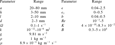
We have several dimensionless parameters in our model and we note that these parameter values can vary greatly in magnitude (table 1). We now make some further assumptions on the size of these parameters relevant to the HARV bioreactor. We first assume that the bioreactor thickness is much smaller than its radius,
 $\unicode[STIX]{x1D716}\ll 1$
, which is an intrinsic characteristic of the HARV bioreactor. We further assume that the flow is dominated by pressure and viscosity rather than inertial effects, so that
 $\unicode[STIX]{x1D716}Re\ll 1$
. However, as we are interested in the effect of a weak inertia on this system, we additionally assume that
 $Re\gg 1$
. We also make some size assumptions on the ratio between the width of the gap between the flat sides of the tissue construct and bioreactor, and the bioreactor thickness, defined as
 $\unicode[STIX]{x1D716}_{1}=(h-d)/(2h)$
. We first assume that this gap is much smaller than the bioreactor thickness, so that
 $\unicode[STIX]{x1D716}_{1}\ll 1$
. To focus on the effect of weak inertia, we additionally assume that the effect of the thin gap between the tissue construct and bioreactor on the flow is much smaller than the effect of inertia, and we take
 $\unicode[STIX]{x1D716}_{1}\ll \unicode[STIX]{x1D716}Re$
. This assumption is strictly stronger than the previous one, and allows us to neglect the role of the thin gap in the reduced flow problem we define below. This assumption will become relevant in appendix A when we derive the effective boundary conditions for the reduced flow problem. Although the gap has a small effect on the flow in the bioreactor, the gap remains important for the trajectory problem because it causes a significant friction between the construct and the bioreactor. Finally, we further assume that the thin gap is smaller than the boundary layers determined in Dalwadi et al. (Reference Dalwadi, Chapman, Waters and Oliver2016) and appendix A, requiring
 $\unicode[STIX]{x1D716}_{1}Re\ll 1$
; thus, the gap does not affect the boundary layer structure and subsequent coupling results.
Typical dimensional (left) and dimensionless (right) parameter values. The absolute upper bound of
 $1/12\approx 8.3\times 10^{-2}$
for
 $K$
can be obtained by considering unobstructed Poiseuille flow through a channel. Data for the HARV operating conditions and construct dimensions are taken from Wolf, Sams & Schwarz (Reference Wolf, Sams and Schwarz1992), Freed & Vunjak-Novakovic (Reference Freed and Vunjak-Novakovic1997), Ingram et al. (Reference Ingram, Techy, Saroufeem, Yazan, Narayan, Goodwin and Spaulding1997), Schwarz & Anderson (Reference Schwarz and Anderson1998), Yu et al. (Reference Yu, Botchwey, Levine, Pollack and Laurencin2004), Cummings et al. (Reference Cummings, Sawyer, Morgan, Rose and Waters2009). Data for construct permeability are taken from Šimáček & Advani (Reference Šimáček and Advani1996), Sucosky et al. (Reference Sucosky, Osorio, Brown and Neitzel2004), Nabovati, Llewellin & Sousa (Reference Nabovati, Llewellin and Sousa2009). We use the standard acceleration due to gravity, and the density and viscosity values of water at room temperature for
 $\unicode[STIX]{x1D70C}$
and
 $\unicode[STIX]{x1D707}$
, respectively. Although the dimensionless groupings can vary significantly in magnitude across the range of rotating bioreactors, we are interested in the HARV bioreactor where
 $\unicode[STIX]{x1D716}$
and
 $\unicode[STIX]{x1D716}_{1}$
are small (Cummings et al.
Reference Cummings, Sawyer, Morgan, Rose and Waters2009).
Additionally, tissue engineering applications require as large a permeability as possible to enhance nutrient delivery to cells, while retaining the structural integrity of the construct. Thus,
 $K$
is on the larger side of its range while still ensuring that Darcy’s law is applicable within the construct. The flow within our construct is governed by Darcy’s law because the underlying solid matrix of our porous medium is connected (Auriault Reference Auriault2009); a tissue construct requires the structural integrity provided by a connected solid matrix. We follow Dalwadi et al. (Reference Dalwadi, Chapman, Waters and Oliver2016) and consider small values of
 $K$
, but do not exploit the asymptotic limit in our analysis. That is, we treat
 $K$
as being of order unity in the asymptotic limits mentioned above for algebraic convenience, rather than scaling
 $K$
with one of these small parameters. The latter treatment would be highly unwieldy, as discussed in Dalwadi et al. (Reference Dalwadi, Chapman, Waters and Oliver2016). Finally, we note that whilst the Bond number can be very large, its large size does not affect our analysis because it is absorbed into the reduced pressure. The Bond number only plays a role in the tissue construct force balance in § 4 where it is multiplied by
 $\unicode[STIX]{x1D716}_{1}$
.
To summarize, the physically relevant asymptotic limit we consider is:
 $\unicode[STIX]{x1D716}\ll 1\ll Re$
,
 $\unicode[STIX]{x1D716}_{1}\ll \unicode[STIX]{x1D716}Re\ll 1$
, and
 $\unicode[STIX]{x1D716}_{1}Re\ll 1$
. We now investigate the coupled system of equations using an asymptotic analysis, requiring matched asymptotic expansions for the flow problem, and a multiple-scales analysis for the trajectory problem. We begin with the flow equations.
3 Flow problem
We now present a formally derived reduced flow problem, and solve this flow problem for a given construct motion. The details of the reduction are sequestered to appendix A as they are similar to those in Dalwadi et al. (Reference Dalwadi, Chapman, Waters and Oliver2016).
We substitute the following asymptotic expansions
 $$\begin{eqnarray}f=f_{0}+\unicode[STIX]{x1D716}Ref_{1}+\mathit{o}(\unicode[STIX]{x1D716}Re),\end{eqnarray}$$
for our flow variables, where
 $f\in \{\boldsymbol{u},\boldsymbol{Q},p,P\}$
, into the governing equations (2.12)–(2.13). We are interested in terms up to
 $O(\unicode[STIX]{x1D716}Re)$
to capture the effects of weak inertia in the problem. We have not expanded the time-dependent functions of construct position
 $R$
,
 $\unicode[STIX]{x1D711}$
, and
 $\unicode[STIX]{x1D714}$
, as we determine in § 4 that the first correction to the construct position is
 $O(\unicode[STIX]{x1D716}_{1})$
, and
 $\unicode[STIX]{x1D716}_{1}\ll \unicode[STIX]{x1D716}Re$
. Therefore, we leave the tissue construct position functions as
 $O(1)$
variables for now, and expand them into smaller correction terms when necessary in § 4.
As the leading-order system is the lubrication equations, we can write the reduced system in terms of the fluid pressure, which have no
 $z$
-dependence. The resulting
 $O(1)$
system is
 $$\begin{eqnarray}\displaystyle & \displaystyle \unicode[STIX]{x1D6FB}_{\bot }^{2}p_{0}=0\quad \text{in }D_{1}, & \displaystyle\end{eqnarray}$$
 $$\begin{eqnarray}\displaystyle & \displaystyle \unicode[STIX]{x1D6FB}_{\bot }^{2}P_{0}=0\quad \text{in }D_{2}, & \displaystyle\end{eqnarray}$$
 $\unicode[STIX]{x1D6FB}_{\bot }^{2}=\unicode[STIX]{x2202}_{XX}+\unicode[STIX]{x2202}_{YY}$
, and we define the domains
 $$\begin{eqnarray}\displaystyle & \displaystyle D_{1}=\{(X,Y)\in \mathbb{R}^{2}:X^{2}+Y^{2}<1,(X-R)^{2}+Y^{2}>b^{2}\}, & \displaystyle\end{eqnarray}$$
 $$\begin{eqnarray}\displaystyle & \displaystyle D_{2}=\{(X,Y)\in \mathbb{R}^{2}:(X-R)^{2}+Y^{2}<b^{2}\}, & \displaystyle\end{eqnarray}$$
The domains of the reduced system and the bipolar transformation defined in (3.8). (a)
 $(X,Y)$
coordinates and (b)
 $(\unicode[STIX]{x1D6FC},\unicode[STIX]{x1D6FD})$
coordinates.

On the curved bioreactor boundary, we have the no-flux condition
 $$\begin{eqnarray}\frac{\unicode[STIX]{x2202}p_{0}}{\unicode[STIX]{x2202}n}=0\quad \text{on }\unicode[STIX]{x2202}D_{1},\end{eqnarray}$$
where
 $\unicode[STIX]{x2202}/\unicode[STIX]{x2202}n$
is the normal derivative directed out of the bioreactor, and on the curved construct boundary we have continuity of pressure and continuity of flux conditions
 $$\begin{eqnarray}\displaystyle & \displaystyle p_{0}-P_{0}=0\quad \text{on }\unicode[STIX]{x2202}D_{2}, & \displaystyle\end{eqnarray}$$
 $$\begin{eqnarray}\displaystyle & \displaystyle -{\displaystyle \frac{1}{12}}\frac{\unicode[STIX]{x2202}p_{0}}{\unicode[STIX]{x2202}n}+K\frac{\unicode[STIX]{x2202}P_{0}}{\unicode[STIX]{x2202}n}={\displaystyle \frac{1}{b}}(\dot{R}(X-R)-(1-\dot{\unicode[STIX]{x1D711}})YR)\quad \text{on }\unicode[STIX]{x2202}D_{2}, & \displaystyle\end{eqnarray}$$
where
 $\unicode[STIX]{x2202}/\unicode[STIX]{x2202}n$
is the normal derivative directed out of the construct. The boundaries in (3.4) are defined as
 $$\begin{eqnarray}\displaystyle & \displaystyle \unicode[STIX]{x2202}D_{1}=\{(X,Y)\in \mathbb{R}^{2}:X^{2}+Y^{2}=1\}, & \displaystyle\end{eqnarray}$$
 $$\begin{eqnarray}\displaystyle & \displaystyle \unicode[STIX]{x2202}D_{2}=\{(X,Y)\in \mathbb{R}^{2}:(X-R)^{2}+Y^{2}=b^{2}\}, & \displaystyle\end{eqnarray}$$
At
 $O(\unicode[STIX]{x1D716}Re)$
, the reduced governing equations are
 $$\begin{eqnarray}\displaystyle & \displaystyle \unicode[STIX]{x1D6FB}_{\bot }^{2}p_{1}=2-{\textstyle \frac{3}{560}}\unicode[STIX]{x1D6FB}_{\bot }^{2}|\unicode[STIX]{x1D735}p_{0}|^{2}\quad \text{in }D_{1}, & \displaystyle\end{eqnarray}$$
 $$\begin{eqnarray}\displaystyle & \displaystyle \unicode[STIX]{x1D6FB}_{\bot }^{2}P_{1}=0\quad \text{in }D_{2}. & \displaystyle\end{eqnarray}$$
 $$\begin{eqnarray}\frac{\unicode[STIX]{x2202}p_{1}}{\unicode[STIX]{x2202}n}=1+{\displaystyle \frac{(1-\dot{\unicode[STIX]{x1D711}})}{10}}\frac{\unicode[STIX]{x2202}}{\unicode[STIX]{x2202}n}\frac{\unicode[STIX]{x2202}p_{0}}{\unicode[STIX]{x2202}s}-{\displaystyle \frac{1}{5}}\frac{\unicode[STIX]{x2202}p_{0}}{\unicode[STIX]{x2202}s}-{\displaystyle \frac{3}{560}}\frac{\unicode[STIX]{x2202}}{\unicode[STIX]{x2202}n}|\unicode[STIX]{x1D735}p_{0}|^{2}\quad \text{on }\unicode[STIX]{x2202}D_{1},\end{eqnarray}$$
with the same notation as for (3.4a
), with the addition of
 $\unicode[STIX]{x2202}/\unicode[STIX]{x2202}s$
, which is the tangential derivative in the anticlockwise direction. That is, with tangential direction
 $\boldsymbol{s}=\boldsymbol{e}_{z}\times \boldsymbol{n}$
on
 $\unicode[STIX]{x2202}D_{1}$
. The numerical prefactors in (3.6a
) and (3.7a
) arise from the averaging of the system over the
 $z$
-direction. The continuity of pressure and continuity of flux conditions on the curved construct boundary are
 $$\begin{eqnarray}p_{1}-P_{1}=\unicode[STIX]{x1D6F1}(s,t)(KP_{0n})^{2}H(-P_{0n})\quad \text{on }\unicode[STIX]{x2202}D_{2},\end{eqnarray}$$
 $$\begin{eqnarray}\displaystyle \frac{\unicode[STIX]{x2202}p_{1}}{\unicode[STIX]{x2202}n}-12K\frac{\unicode[STIX]{x2202}P_{1}}{\unicode[STIX]{x2202}n} & = & \displaystyle \boldsymbol{n}\boldsymbol{\cdot }\boldsymbol{X}^{\bot }-{\displaystyle \frac{3}{560}}\frac{\unicode[STIX]{x2202}}{\unicode[STIX]{x2202}n}|\unicode[STIX]{x1D735}p_{0}|^{2}+{\displaystyle \frac{\boldsymbol{n}\boldsymbol{\cdot }\boldsymbol{B}(s,t)}{10}}\nonumber\\ \displaystyle & & \displaystyle -\,{\displaystyle \frac{\unicode[STIX]{x2202}}{\unicode[STIX]{x2202}s}}(12KP_{0n}\{p_{0s}\unicode[STIX]{x1D6EC}_{a}+\boldsymbol{s}\boldsymbol{\cdot }\boldsymbol{u}^{slip}\unicode[STIX]{x1D6EC}_{b}\})H(-P_{0n})\quad \text{on }\unicode[STIX]{x2202}D_{2},\qquad\end{eqnarray}$$
with the same notation as for (3.4), with the addition of:
 $\unicode[STIX]{x2202}/\unicode[STIX]{x2202}s$
, the tangential derivative in the anticlockwise direction;
 $\unicode[STIX]{x1D6F1}$
, a function of space and time that arises due to the pressure change close to the construct surface (defined in (A 11) and (A 16));
 $\unicode[STIX]{x1D6EC}_{a}$
and
 $\unicode[STIX]{x1D6EC}_{b}$
, functions of space and time that arise due to the movement of fluid close to the construct surface in the direction tangential to the surface (defined in (A 11) and (A 17));
 $H(x)$
, the Heaviside function;
 $\boldsymbol{B}$
, which arises from an inertial correction and is defined in (A 31b
); and
 $\boldsymbol{u}^{slip}$
, the velocity of the bioreactor walls relative to the construct defined in (A 9a
).
3.1 Solution at leading order:
 $O(1)$

The leading-order system is defined by (3.2) and (3.4). We follow Cummings & Waters (Reference Cummings and Waters2007), who consider a similar system, and transform to bipolar coordinates
 $(\unicode[STIX]{x1D6FC},\unicode[STIX]{x1D6FD})$
, defined by
 $$\begin{eqnarray}X=\cosh \unicode[STIX]{x1D6FC}_{1}-{\displaystyle \frac{\sinh \unicode[STIX]{x1D6FC}_{1}\sinh \unicode[STIX]{x1D6FC}}{\cosh \unicode[STIX]{x1D6FC}-\cos \unicode[STIX]{x1D6FD}}},\quad Y={\displaystyle \frac{\sinh \unicode[STIX]{x1D6FC}_{1}\sin \unicode[STIX]{x1D6FD}}{\cosh \unicode[STIX]{x1D6FC}-\cos \unicode[STIX]{x1D6FD}}},\end{eqnarray}$$
where
 $$\begin{eqnarray}b={\displaystyle \frac{\sinh \unicode[STIX]{x1D6FC}_{1}}{\sinh \unicode[STIX]{x1D6FC}_{2}}},\quad R=\cosh \unicode[STIX]{x1D6FC}_{1}-\sinh \unicode[STIX]{x1D6FC}_{1}\coth \unicode[STIX]{x1D6FC}_{2}.\end{eqnarray}$$
The bipolar transformation is useful here as it transforms the domain of two non-concentric circles, one contained within the other, to a rectangular domain, allowing us to obtain an analytic solution. We show a schematic of the transformed domains in figure 3(b). The bulk flow region now corresponds to the finite rectangle defined by
 $0<\unicode[STIX]{x1D6FC}_{1}<\unicode[STIX]{x1D6FC}<\unicode[STIX]{x1D6FC}_{2}$
and
 $0<\unicode[STIX]{x1D6FD}<2\unicode[STIX]{x03C0}$
, and the porous region corresponds to the semi-infinite rectangle defined by
 $\unicode[STIX]{x1D6FC}_{2}<\unicode[STIX]{x1D6FC}<\infty$
and
 $0<\unicode[STIX]{x1D6FD}<2\unicode[STIX]{x03C0}$
. Additionally, both regions now require periodic boundary conditions at
 $\unicode[STIX]{x1D6FD}=0$
and
 $2\unicode[STIX]{x03C0}$
. Hence, the bioreactor boundary
 $\unicode[STIX]{x2202}D_{1}$
corresponds to
 $\unicode[STIX]{x1D6FC}=\unicode[STIX]{x1D6FC}_{1}$
, and the tissue construct boundary
 $\unicode[STIX]{x2202}D_{2}$
corresponds to
 $\unicode[STIX]{x1D6FC}=\unicode[STIX]{x1D6FC}_{2}$
. On both
 $\unicode[STIX]{x2202}D_{1}$
and
 $\unicode[STIX]{x2202}D_{2}$
, we find that
 $\boldsymbol{n}=-\boldsymbol{e}_{\unicode[STIX]{x1D6FC}}$
and
 $\boldsymbol{s}=-\boldsymbol{e}_{\unicode[STIX]{x1D6FD}}$
.
Laplace’s equation in (3.2) is invariant under the conformal bipolar transformation, and these governing equations must be solved subject to the boundary condition (3.4a
) on
 $\unicode[STIX]{x1D6FC}=\unicode[STIX]{x1D6FC}_{1}$
, given by
 $$\begin{eqnarray}\frac{\unicode[STIX]{x2202}p_{0}}{\unicode[STIX]{x2202}\unicode[STIX]{x1D6FC}}=0,\end{eqnarray}$$
along with the coupling conditions (3.4b
) and (3.4c
) on
 $\unicode[STIX]{x1D6FC}=\unicode[STIX]{x1D6FC}_{2}$
, which become
 $$\begin{eqnarray}\displaystyle & \displaystyle p_{0}=P_{0}, & \displaystyle\end{eqnarray}$$
 $$\begin{eqnarray}\displaystyle & \displaystyle -{\displaystyle \frac{1}{12}}\frac{\unicode[STIX]{x2202}p_{0}}{\unicode[STIX]{x2202}\unicode[STIX]{x1D6FC}}+K\frac{\unicode[STIX]{x2202}P_{0}}{\unicode[STIX]{x2202}\unicode[STIX]{x1D6FC}}={\displaystyle \frac{\sinh \unicode[STIX]{x1D6FC}_{1}(R(1-\dot{\unicode[STIX]{x1D711}})\sin \unicode[STIX]{x1D6FD}\sinh \unicode[STIX]{x1D6FC}_{2}+\dot{R}(\cos \unicode[STIX]{x1D6FD}\cosh \unicode[STIX]{x1D6FC}_{2}-1))}{(\cosh \unicode[STIX]{x1D6FC}_{2}-\cos \unicode[STIX]{x1D6FD})^{2}}}. & \displaystyle \nonumber\\ \displaystyle & & \displaystyle\end{eqnarray}$$
The system (3.2), (3.10)–(3.11) is solved by
 $$\begin{eqnarray}\displaystyle & \displaystyle p_{0}=\mathop{\sum }_{n=1}^{\infty }[A_{n}\cos n\unicode[STIX]{x1D6FD}+B_{n}\sin n\unicode[STIX]{x1D6FD}]\cosh n(\unicode[STIX]{x1D6FC}-\unicode[STIX]{x1D6FC}_{1}), & \displaystyle\end{eqnarray}$$
 $$\begin{eqnarray}\displaystyle & \displaystyle P_{0}=\mathop{\sum }_{n=1}^{\infty }[C_{n}\cos n\unicode[STIX]{x1D6FD}+D_{n}\sin n\unicode[STIX]{x1D6FD}]\text{e}^{-n(\unicode[STIX]{x1D6FC}-\unicode[STIX]{x1D6FC}_{2})}, & \displaystyle\end{eqnarray}$$
 $A_{n}$
,
 $B_{n}$
,
 $C_{n}$
, and
 $D_{n}$
are given by
 $$\begin{eqnarray}\left.\begin{array}{@{}c@{}}\displaystyle A_{n}=L_{n}\dot{R}\operatorname{sech}n(\unicode[STIX]{x1D6FC}_{2}-\unicode[STIX]{x1D6FC}_{1}),\quad B_{n}=L_{n}R(1-\dot{\unicode[STIX]{x1D711}})\operatorname{sech}n(\unicode[STIX]{x1D6FC}_{2}-\unicode[STIX]{x1D6FC}_{1}),\\ \displaystyle C_{n}=L_{n}\dot{R},\quad D_{n}=L_{n}R(1-\dot{\unicode[STIX]{x1D711}}),\quad L_{n}=-{\displaystyle \frac{24\sinh \unicode[STIX]{x1D6FC}_{1}\text{e}^{-n\unicode[STIX]{x1D6FC}_{2}}}{\tanh n(\unicode[STIX]{x1D6FC}_{2}-\unicode[STIX]{x1D6FC}_{1})+12K}}.\end{array}\right\}\end{eqnarray}$$
In Cummings & Waters (Reference Cummings and Waters2007), a solid tissue construct is considered. In the limit of
 $K\rightarrow 0$
, corresponding to a solid tissue construct, the coefficients
 $A_{n}$
and
 $B_{n}$
in (3.13) tend to those obtained in Cummings & Waters (Reference Cummings and Waters2007).
3.2 Solution at first correction:
$O(\unicode[STIX]{x1D716}Re)$

We now solve the
 $O(\unicode[STIX]{x1D716}Re)$
system, given by (3.6)–(3.7), again using the bipolar transformation (3.8). We introduce
 $$\begin{eqnarray}\unicode[STIX]{x1D6F9}=p_{1}-{\displaystyle \frac{1}{2}}(X^{2}+Y^{2})+{\displaystyle \frac{3}{560}}|\unicode[STIX]{x1D735}p_{0}|^{2},\end{eqnarray}$$
and note that Laplace’s equation in (3.6) is invariant under the conformal bipolar transformation, yielding the governing equations
 $$\begin{eqnarray}\displaystyle & \displaystyle \unicode[STIX]{x1D6FB}_{\bot }^{2}\unicode[STIX]{x1D6F9}=0\quad \unicode[STIX]{x1D6FC}_{1}<\unicode[STIX]{x1D6FC}<\unicode[STIX]{x1D6FC}_{2},\quad 0<\unicode[STIX]{x1D6FD}<2\unicode[STIX]{x03C0}, & \displaystyle\end{eqnarray}$$
 $$\begin{eqnarray}\displaystyle & \displaystyle \unicode[STIX]{x1D6FB}_{\bot }^{2}P_{1}=0\quad \unicode[STIX]{x1D6FC}_{2}<\unicode[STIX]{x1D6FC}<\infty ,\quad 0<\unicode[STIX]{x1D6FD}<2\unicode[STIX]{x03C0}. & \displaystyle\end{eqnarray}$$
 $$\begin{eqnarray}\frac{\unicode[STIX]{x2202}\unicode[STIX]{x1D6F9}}{\unicode[STIX]{x2202}n}={\displaystyle \frac{(1-\dot{\unicode[STIX]{x1D711}})}{10}}\frac{\unicode[STIX]{x2202}}{\unicode[STIX]{x2202}n}\frac{\unicode[STIX]{x2202}p_{0}}{\unicode[STIX]{x2202}s}-{\displaystyle \frac{1}{5}}\frac{\unicode[STIX]{x2202}p_{0}}{\unicode[STIX]{x2202}s}\quad \text{on }\unicode[STIX]{x2202}D_{1},\end{eqnarray}$$
and the continuity of pressure (3.7b ) and continuity of flux (3.7c ) conditions at the construct interface become
 $$\begin{eqnarray}\unicode[STIX]{x1D6F9}-P_{1}=-{\displaystyle \frac{X^{2}+Y^{2}}{2}}+{\displaystyle \frac{3|\unicode[STIX]{x1D735}p_{0}|^{2}}{560}}+\unicode[STIX]{x1D6F1}(s,t)(KP_{0n})^{2}H(-P_{0n})\quad \text{on }\unicode[STIX]{x2202}D_{2},\end{eqnarray}$$
 $$\begin{eqnarray}\displaystyle \frac{\unicode[STIX]{x2202}\unicode[STIX]{x1D6F9}}{\unicode[STIX]{x2202}n}-12K\frac{\unicode[STIX]{x2202}P_{1}}{\unicode[STIX]{x2202}n} & = & \displaystyle {\displaystyle \frac{\boldsymbol{n}\boldsymbol{\cdot }\boldsymbol{B}(s,t)}{10}}\nonumber\\ \displaystyle & & \displaystyle -\,{\displaystyle \frac{\unicode[STIX]{x2202}}{\unicode[STIX]{x2202}s}}(12KP_{0n}\{p_{0s}\unicode[STIX]{x1D6EC}_{a}+\boldsymbol{s}\boldsymbol{\cdot }\boldsymbol{u}^{slip}\unicode[STIX]{x1D6EC}_{b}\})H(-P_{0n})\quad \text{on }\unicode[STIX]{x2202}D_{2},\qquad\end{eqnarray}$$
where
 $\boldsymbol{B}$
is defined in (A 31b
),
 $H(x)$
is the Heaviside function,
 $\boldsymbol{u}^{slip}$
is the velocity of the bioreactor walls relative to the construct defined in (A 9a
).
As with the
 $O(1)$
equations, it is convenient to solve this problem in terms of Fourier series by transforming to the bipolar coordinate system described by (3.8)–(3.9). Thus, we rewrite our boundary conditions as
 $$\begin{eqnarray}\displaystyle & \displaystyle \frac{\unicode[STIX]{x2202}\unicode[STIX]{x1D6F9}}{\unicode[STIX]{x2202}n}=-{\displaystyle \frac{\cosh \unicode[STIX]{x1D6FC}_{1}-\cos \unicode[STIX]{x1D6FD}}{\sinh \unicode[STIX]{x1D6FC}_{1}}}\left(a_{10}+\mathop{\sum }_{n=1}^{\infty }(a_{1n}\cos n\unicode[STIX]{x1D6FD}+b_{1n}\sin n\unicode[STIX]{x1D6FD})\right)\quad \text{on }\unicode[STIX]{x2202}D_{1},\qquad & \displaystyle\end{eqnarray}$$
 $$\begin{eqnarray}\displaystyle & \displaystyle \unicode[STIX]{x1D6F9}-P_{1}=a_{20}+\mathop{\sum }_{n=1}^{\infty }(a_{2n}\cos n\unicode[STIX]{x1D6FD}+b_{2n}\sin n\unicode[STIX]{x1D6FD})\quad \text{on }\unicode[STIX]{x2202}D_{2}, & \displaystyle\end{eqnarray}$$
 $$\begin{eqnarray}\displaystyle \frac{\unicode[STIX]{x2202}\unicode[STIX]{x1D6F9}}{\unicode[STIX]{x2202}n}-12K\frac{\unicode[STIX]{x2202}P_{1}}{\unicode[STIX]{x2202}n} & = & \displaystyle -{\displaystyle \frac{\cosh \unicode[STIX]{x1D6FC}_{2}-\cos \unicode[STIX]{x1D6FD}}{\sinh \unicode[STIX]{x1D6FC}_{1}}}\nonumber\\ \displaystyle & & \displaystyle \times \,\left(a_{30}+\displaystyle \mathop{\sum }_{n=1}^{\infty }(a_{3n}\cos n\unicode[STIX]{x1D6FD}+b_{3n}\sin n\unicode[STIX]{x1D6FD})\right)\quad \text{on }\unicode[STIX]{x2202}D_{2},\end{eqnarray}$$
 $a_{in}(t)$
and
 $b_{in}(t)$
, for
 $i\in \{1,2,3\}$
, can be determined by comparison with the corresponding boundary conditions (3.16). We note that
 $a_{in}$
and
 $b_{in}$
are functions of time, but are independent of
 $\unicode[STIX]{x1D6FC}$
and
 $\unicode[STIX]{x1D6FD}$
. Additionally, to ensure consistency in our system, we have the solvability conditions
 $a_{10}=a_{30}$
and
 $\int _{\unicode[STIX]{x2202}D_{2}}\unicode[STIX]{x2202}P_{1}/\unicode[STIX]{x2202}n\,\text{d}s=0$
, arising from conservation of mass. As (3.16a
) is linear in the leading-order pressure, the
 $a_{1n}(t)$
and
 $b_{1n}(t)$
terms can be determined easily from (3.12a
), (3.16a
), and (3.17a
) as follows
 $$\begin{eqnarray}a_{10}=0,\quad a_{1n}(t)={\displaystyle \frac{\dot{\unicode[STIX]{x1D711}}-3}{10}}nB_{n},\quad b_{1n}(t)={\displaystyle \frac{3-\dot{\unicode[STIX]{x1D711}}}{10}}nA_{n}.\end{eqnarray}$$
However, the expressions for
 $a_{2n}$
,
 $a_{3n}$
,
 $b_{2n}$
, and
 $b_{3n}$
are not as easily expressible in terms of analytically known coefficients; hence we determine these numerically.
The solution to (3.15) and (3.17) is
 $$\begin{eqnarray}\displaystyle & \displaystyle \unicode[STIX]{x1D6F9}=\unicode[STIX]{x1D6F9}_{1}+\unicode[STIX]{x1D6F9}_{2}, & \displaystyle\end{eqnarray}$$
 $$\begin{eqnarray}\displaystyle & \displaystyle P_{1}=\mathop{\sum }_{n=1}^{\infty }[\overline{E}_{n}\cos n\unicode[STIX]{x1D6FD}+\overline{F}_{n}\sin n\unicode[STIX]{x1D6FD}]\text{e}^{-n(\unicode[STIX]{x1D6FC}-\unicode[STIX]{x1D6FC}_{2})}, & \displaystyle\end{eqnarray}$$
 $$\begin{eqnarray}\displaystyle & \displaystyle \unicode[STIX]{x1D6F9}_{1}=\mathop{\sum }_{n=1}^{\infty }[\overline{A}_{n}\cos n\unicode[STIX]{x1D6FD}+\overline{B}_{n}\sin n\unicode[STIX]{x1D6FD}]\cosh n(\unicode[STIX]{x1D6FC}-\unicode[STIX]{x1D6FC}_{2}), & \displaystyle\end{eqnarray}$$
 $$\begin{eqnarray}\displaystyle & \displaystyle \unicode[STIX]{x1D6F9}_{2}=a_{10}(\unicode[STIX]{x1D6FC}-\unicode[STIX]{x1D6FC}_{2})+a_{20}+\mathop{\sum }_{n=1}^{\infty }[\overline{C}_{n}\cos n\unicode[STIX]{x1D6FD}+\overline{D}_{n}\sin n\unicode[STIX]{x1D6FD}]\sinh n(\unicode[STIX]{x1D6FC}-\unicode[STIX]{x1D6FC}_{2}), & \displaystyle\end{eqnarray}$$
 $\overline{A}_{n}$
,
 $\overline{B}_{n}$
,
 $\overline{C}_{n}$
,
 $\overline{D}_{n}$
,
 $\overline{E}_{n}$
, and
 $\overline{F}_{n}$
are given by
 $$\begin{eqnarray}\displaystyle & \displaystyle \overline{A}_{n}=\overline{L}_{n}(a_{3n}-a_{1n}\operatorname{sech}n(\unicode[STIX]{x1D6FC}_{2}-\unicode[STIX]{x1D6FC}_{1})+12Kna_{2n}), & \displaystyle\end{eqnarray}$$
 $$\begin{eqnarray}\displaystyle & \displaystyle \overline{B}_{n}=\overline{L}_{n}(b_{3n}-b_{1n}\operatorname{sech}n(\unicode[STIX]{x1D6FC}_{2}-\unicode[STIX]{x1D6FC}_{1})+12Knb_{2n}), & \displaystyle\end{eqnarray}$$
 $$\begin{eqnarray}\displaystyle & \displaystyle \overline{C}_{n}=\overline{L}_{n}((a_{3n}+12Kna_{2n})\tanh n(\unicode[STIX]{x1D6FC}_{2}-\unicode[STIX]{x1D6FC}_{1})+12Ka_{1n}\operatorname{sech}n(\unicode[STIX]{x1D6FC}_{2}-\unicode[STIX]{x1D6FC}_{1})), & \displaystyle\end{eqnarray}$$
 $$\begin{eqnarray}\displaystyle & \displaystyle \overline{D}_{n}=\overline{L}_{n}((b_{3n}+12Knb_{2n})\tanh n(\unicode[STIX]{x1D6FC}_{2}-\unicode[STIX]{x1D6FC}_{1})+12Kb_{1n}\operatorname{sech}n(\unicode[STIX]{x1D6FC}_{2}-\unicode[STIX]{x1D6FC}_{1})), & \displaystyle\end{eqnarray}$$
 $$\begin{eqnarray}\displaystyle & \displaystyle \overline{E}_{n}=\overline{L}_{n}(a_{3n}-a_{1n}\operatorname{sech}n(\unicode[STIX]{x1D6FC}_{2}-\unicode[STIX]{x1D6FC}_{1})-na_{2n}\tanh n(\unicode[STIX]{x1D6FC}_{2}-\unicode[STIX]{x1D6FC}_{1})), & \displaystyle\end{eqnarray}$$
 $$\begin{eqnarray}\displaystyle & \displaystyle \overline{F}_{n}=\overline{L}_{n}(b_{3n}-b_{1n}\operatorname{sech}n(\unicode[STIX]{x1D6FC}_{2}-\unicode[STIX]{x1D6FC}_{1})-nb_{2n}\tanh n(\unicode[STIX]{x1D6FC}_{2}-\unicode[STIX]{x1D6FC}_{1})), & \displaystyle\end{eqnarray}$$
 $$\begin{eqnarray}\displaystyle & \displaystyle \overline{L}_{n}=1/(n(\tanh n(\unicode[STIX]{x1D6FC}_{2}-\unicode[STIX]{x1D6FC}_{1})+12K)), & \displaystyle\end{eqnarray}$$
 $O(\unicode[STIX]{x1D716}Re)$
. We now investigate the motion of the tissue construct.
4 Tissue construct motion
The dimensionless tissue construct motion problem is presented in (2.16). To obtain the correct hydrodynamic contributions to the force and torque we consider the relevant asymptotic regions for the flow in appendix A.
We start with
 $\boldsymbol{f}_{f}$
and
 $\unicode[STIX]{x1D749}_{f}$
, the force and torque, respectively, on the flat sides of the construct. We consider the flow between the flat sides of the tissue construct and bioreactor in § A.1, and we determine that the effective hydrodynamical stress is
 $$\begin{eqnarray}\unicode[STIX]{x1D748}\boldsymbol{\cdot }\boldsymbol{n}={\displaystyle \frac{\unicode[STIX]{x1D716}}{\unicode[STIX]{x1D716}_{1}}}(-\dot{R}\boldsymbol{e}_{X}+R(1-\dot{\unicode[STIX]{x1D711}})\boldsymbol{e}_{Y}+(1-\unicode[STIX]{x1D714})\boldsymbol{e}_{z}\times \boldsymbol{r})+O(\unicode[STIX]{x1D716}\unicode[STIX]{x1D716}_{1})\quad \text{on }T_{2}\cup T_{3},\end{eqnarray}$$
where
 $\boldsymbol{n}$
is the unit normal directed out of the construct, and thus this stress acts to oppose the motion of the tissue construct relative to the bioreactor as a frictional effect. It is a simple task to determine
 $$\begin{eqnarray}\displaystyle & \displaystyle \boldsymbol{f}_{f}=2\unicode[STIX]{x03C0}b^{2}{\displaystyle \frac{\unicode[STIX]{x1D716}}{\unicode[STIX]{x1D716}_{1}}}(-\dot{R}\boldsymbol{e}_{X}+R(1-\dot{\unicode[STIX]{x1D711}})\boldsymbol{e}_{Y})+O(\unicode[STIX]{x1D716}\unicode[STIX]{x1D716}_{1}), & \displaystyle\end{eqnarray}$$
 $$\begin{eqnarray}\displaystyle & \displaystyle \unicode[STIX]{x1D749}_{f}=\unicode[STIX]{x03C0}b^{4}{\displaystyle \frac{\unicode[STIX]{x1D716}}{\unicode[STIX]{x1D716}_{1}}}(1-\unicode[STIX]{x1D714})\boldsymbol{e}_{z}+O(\unicode[STIX]{x1D716}\unicode[STIX]{x1D716}_{1}). & \displaystyle\end{eqnarray}$$
We now consider
 $\boldsymbol{f}_{c}$
and
 $\unicode[STIX]{x1D749}_{c}$
, the force and torque, respectively, on the curved sides of the construct. We consider the flow near the curved interface in appendix A, and we determine that the effective hydrodynamical stress on
 $T_{1}$
is
 $$\begin{eqnarray}\displaystyle \unicode[STIX]{x1D748}\boldsymbol{\cdot }\boldsymbol{n} & = & \displaystyle B(X\sin \unicode[STIX]{x1D711}+Y\cos \unicode[STIX]{x1D711})\boldsymbol{n}-(P_{0}+\unicode[STIX]{x1D716}ReP_{1})\boldsymbol{n}\nonumber\\ \displaystyle & & \displaystyle -\,\unicode[STIX]{x1D716}Re(\boldsymbol{u}_{0}^{rel}\boldsymbol{\cdot }\boldsymbol{n})(\boldsymbol{u}_{0}^{rel}\boldsymbol{\cdot }\boldsymbol{s})H(P_{0n})\boldsymbol{s}+O(\unicode[STIX]{x1D716}Re^{1/2}),\end{eqnarray}$$
where
 $H(x)$
is the Heaviside function,
 $\boldsymbol{s}$
is the unit tangent vector directed anticlockwise around the construct, and
 $$\begin{eqnarray}\boldsymbol{u}_{0}^{rel}=-\dot{R}\boldsymbol{e}_{X}+R(1-\dot{\unicode[STIX]{x1D711}})\boldsymbol{e}_{Y}+(1-\unicode[STIX]{x1D714})\boldsymbol{e}_{z}\times \boldsymbol{r}+f_{1}(z)\unicode[STIX]{x1D735}p_{0}.\end{eqnarray}$$
The first term on the right-hand side of (4.3) arises from the definition of the reduced pressure in § 2.2, causing the buoyancy force acting on the tissue construct. The term in the tangential direction on the right-hand side of (4.3) arises from the boundary layer analysis in appendix A.
Using (4.3) and transforming the integrals into the bipolar coordinate system we use to solve the flow problem, we deduce that
 $$\begin{eqnarray}\displaystyle \boldsymbol{f}_{c} & = & \displaystyle \unicode[STIX]{x1D716}B{\mathcal{V}}(\sin \unicode[STIX]{x1D711}\boldsymbol{e}_{X}+\cos \unicode[STIX]{x1D711}\boldsymbol{e}_{Y})-\unicode[STIX]{x1D716}{\mathcal{V}}{\displaystyle \frac{\sinh \unicode[STIX]{x1D6FC}_{1}}{\unicode[STIX]{x03C0}b^{2}}}\int _{0}^{2\unicode[STIX]{x03C0}}{\displaystyle \frac{P_{0}+\unicode[STIX]{x1D716}ReP_{1}}{\cosh \unicode[STIX]{x1D6FC}_{2}-\cos \unicode[STIX]{x1D6FD}}}\boldsymbol{n}\,\text{d}\unicode[STIX]{x1D6FD}\nonumber\\ \displaystyle & & \displaystyle -\,\unicode[STIX]{x1D716}^{2}Re\sinh \unicode[STIX]{x1D6FC}_{1}\int _{0}^{2\unicode[STIX]{x03C0}}\int _{0}^{1}{\displaystyle \frac{(\boldsymbol{u}_{0}^{rel}\boldsymbol{\cdot }\boldsymbol{n})(\boldsymbol{u}_{0}^{rel}\boldsymbol{\cdot }\boldsymbol{s})H(P_{0n})}{\cosh \unicode[STIX]{x1D6FC}_{2}-\cos \unicode[STIX]{x1D6FD}}}\boldsymbol{s}\,\text{d}z\,\text{d}\unicode[STIX]{x1D6FD}+O(\unicode[STIX]{x1D716}^{2}Re^{1/2}),\end{eqnarray}$$
 $$\begin{eqnarray}\unicode[STIX]{x1D749}_{c}=-\unicode[STIX]{x1D716}^{2}Reb\sinh \unicode[STIX]{x1D6FC}_{1}\boldsymbol{e}_{z}\int _{0}^{2\unicode[STIX]{x03C0}}\int _{0}^{1}{\displaystyle \frac{(\boldsymbol{u}_{0}^{rel}\boldsymbol{\cdot }\boldsymbol{n})(\boldsymbol{u}_{0}^{rel}\boldsymbol{\cdot }\boldsymbol{s})H(P_{0n})}{(\cosh \unicode[STIX]{x1D6FC}_{2}-\cos \unicode[STIX]{x1D6FD})^{2}}}\,\text{d}z\,\text{d}\unicode[STIX]{x1D6FD}+O(\unicode[STIX]{x1D716}^{2}Re^{1/2}),\end{eqnarray}$$
 $\unicode[STIX]{x1D6FC}=\unicode[STIX]{x1D6FC}_{2}$
. Moreover, we are able to directly calculate the pressure integral in (4.5a
) from the solutions to
 $P_{0}$
and
 $P_{1}$
(given in (3.12b
) and (3.19b
)). We find that
 $$\begin{eqnarray}{\displaystyle \frac{\sinh \unicode[STIX]{x1D6FC}_{1}}{\unicode[STIX]{x03C0}b^{2}}}\int _{0}^{2\unicode[STIX]{x03C0}}{\displaystyle \frac{P_{0}(\unicode[STIX]{x1D6FC}_{2},\unicode[STIX]{x1D6FD})}{\cosh \unicode[STIX]{x1D6FC}_{2}-\cos \unicode[STIX]{x1D6FD}}}\boldsymbol{n}\,\text{d}\unicode[STIX]{x1D6FD}=2(\dot{R}\boldsymbol{e}_{X}-R(1-\dot{\unicode[STIX]{x1D711}})\boldsymbol{e}_{Y})\unicode[STIX]{x1D6FE}_{1}(R),\end{eqnarray}$$
where
 $$\begin{eqnarray}\unicode[STIX]{x1D6FE}_{1}(R)=24\sinh ^{2}\unicode[STIX]{x1D6FC}_{2}\mathop{\sum }_{n=1}^{\infty }{\displaystyle \frac{n\text{e}^{-2n\unicode[STIX]{x1D6FC}_{2}}}{\tanh n(\unicode[STIX]{x1D6FC}_{2}-\unicode[STIX]{x1D6FC}_{1})+12K}},\end{eqnarray}$$
noting that
 $\unicode[STIX]{x1D6FC}_{1}$
and
 $\unicode[STIX]{x1D6FC}_{2}$
are functions of
 $R$
, and
 $\unicode[STIX]{x1D6FE}_{1}(R)$
is a monotonically increasing function of
 $R$
, as shown in figure 4 for various values of the dimensionless permeability
 $K$
.
The function
 $\unicode[STIX]{x1D6FE}_{1}(R)$
for various values of
 $K$
, using
 $b=0.2$
. The functions stop at
 $R=1-b$
, which corresponds to where the tissue construct hits the bioreactor edge. The dashed lines are the small
 $R$
asymptotic solutions, and the dotted lines are the small
 $1-b-R$
solutions, both given in (4.7).

We are able to determine the asymptotic behaviour of
 $\unicode[STIX]{x1D6FE}_{1}$
in appendix B as
 $$\begin{eqnarray}\unicode[STIX]{x1D6FE}_{1}\sim {\displaystyle \frac{6}{12K+(1-b^{2})/(1+b^{2})}}\quad \text{as }R\rightarrow 0^{+},\end{eqnarray}$$
 $$\begin{eqnarray}\displaystyle \unicode[STIX]{x1D6FE}_{1} & {\sim} & \displaystyle {\displaystyle \frac{6}{1+12K}}+{\displaystyle \frac{24}{(1-b)^{2}}}\left\{{\displaystyle \frac{\unicode[STIX]{x1D6F7}\displaystyle \left({\displaystyle \frac{1-12K}{1+12K}},2,{\displaystyle \frac{2-b}{1-b}}\right)}{2(1+12K)^{2}}}\right.\nonumber\\ \displaystyle & & \displaystyle +\,12K\log \left(1+\sqrt{{\displaystyle \frac{2(1-b)(1-b-R)}{72bK^{2}}}}\right)\nonumber\\ \displaystyle & & \displaystyle -\,\left.\sqrt{{\displaystyle \frac{(1-b)(1-b-R)}{2b}}}{\displaystyle \frac{\sqrt{(1-b)(1-b-R)}+12K\sqrt{2b}}{\sqrt{(1-b)(1-b-R)}+6K\sqrt{2b}}}\right\}\quad \text{as }R\rightarrow (1-b)^{-},\nonumber\\ \displaystyle & & \displaystyle\end{eqnarray}$$
 $\unicode[STIX]{x1D6F7}(z,s,v)$
, the Lerch transcendent, is defined in (B 8). These asymptotic solutions can be used to efficiently evaluate
 $\unicode[STIX]{x1D6FE}_{1}$
near each limit. As the number of modes required to accurately evaluate
 $\unicode[STIX]{x1D6FE}_{1}$
increases as
 $R\rightarrow (1-b)^{-}$
, the asymptotic solution is particularly useful in this limit. The small
 $R$
asymptotic behaviour persists for non-small
 $R$
, whereas the small
 $1-b-R$
asymptotic behaviour is only a good approximation to the infinite sum very close to the limit (figure 4). In Cummings & Waters (Reference Cummings and Waters2007) it is correctly noted that the flow analysis would not be valid in the limit of
 $R\rightarrow (1-b)^{-}$
as the separation of length scales required for the lubrication assumption to hold would break down. However, it is incorrectly hypothesized that
 $\unicode[STIX]{x1D6FE}_{1}$
is unbounded in the same limit for
 $K=0$
, as our solution (4.7b
) shows that
 $\unicode[STIX]{x1D6FE}_{1}$
is bounded in this limit. Moreover, when
 $K=0$
, note that the Lerch transcendent in (4.7b
) reduces to the polygamma function of order 1, which is sometimes referred to as the trigamma function.
To calculate (4.5a ), we additionally deduce that
 $$\begin{eqnarray}\displaystyle & \displaystyle {\displaystyle \frac{\sinh \unicode[STIX]{x1D6FC}_{1}}{\unicode[STIX]{x03C0}b^{2}}}\int _{0}^{2\unicode[STIX]{x03C0}}{\displaystyle \frac{P_{1}(\unicode[STIX]{x1D6FC}_{2},\unicode[STIX]{x1D6FD})}{\cosh \unicode[STIX]{x1D6FC}_{2}-\cos \unicode[STIX]{x1D6FD}}}\boldsymbol{n}\,\text{d}\unicode[STIX]{x1D6FD}=-2(\unicode[STIX]{x1D6FE}_{2}\boldsymbol{e}_{X}-\unicode[STIX]{x1D6FE}_{3}\boldsymbol{e}_{Y}), & \displaystyle\end{eqnarray}$$
 $$\begin{eqnarray}\displaystyle & \displaystyle \unicode[STIX]{x1D6FE}_{2}={\displaystyle \frac{\sinh \unicode[STIX]{x1D6FC}_{2}}{b}}\mathop{\sum }_{n=1}^{\infty }n\text{e}^{-n\unicode[STIX]{x1D6FC}_{2}}\overline{E}_{n},\quad \unicode[STIX]{x1D6FE}_{3}={\displaystyle \frac{\sinh \unicode[STIX]{x1D6FC}_{2}}{b}}\mathop{\sum }_{n=1}^{\infty }n\text{e}^{-n\unicode[STIX]{x1D6FC}_{2}}\overline{F}_{n}, & \displaystyle\end{eqnarray}$$
where
 $\overline{E}_{n}$
and
 $\overline{F}_{n}$
are defined in (3.20). We note that
 $\unicode[STIX]{x1D6FE}_{2}$
and
 $\unicode[STIX]{x1D6FE}_{3}$
will be functions of the construct motion. It will also be helpful to define the components of the integral in (4.5a
) in the
 $\boldsymbol{e}_{X}$
and
 $\boldsymbol{e}_{Y}$
directions. Noting that
 $\boldsymbol{s}=-\boldsymbol{e}_{\unicode[STIX]{x1D6FD}}$
, which can be written in terms of
 $\boldsymbol{e}_{X}$
and
 $\boldsymbol{e}_{Y}$
, we write
 $$\begin{eqnarray}\unicode[STIX]{x1D6FE}_{4}\boldsymbol{e}_{X}+\unicode[STIX]{x1D6FE}_{5}\boldsymbol{e}_{Y}=-{\displaystyle \frac{\sinh \unicode[STIX]{x1D6FC}_{1}}{2\unicode[STIX]{x03C0}b^{2}}}\int _{0}^{2\unicode[STIX]{x03C0}}\int _{0}^{1}{\displaystyle \frac{(\boldsymbol{u}_{0}^{rel}\boldsymbol{\cdot }\boldsymbol{n})(\boldsymbol{u}_{0}^{rel}\boldsymbol{\cdot }\boldsymbol{s})H(P_{0n})}{\cosh \unicode[STIX]{x1D6FC}_{2}-\cos \unicode[STIX]{x1D6FD}}}\boldsymbol{s}\,\text{d}z\,\text{d}\unicode[STIX]{x1D6FD},\end{eqnarray}$$
where
 $$\begin{eqnarray}\displaystyle & \displaystyle \unicode[STIX]{x1D6FE}_{4}={\displaystyle \frac{\sinh ^{2}\unicode[STIX]{x1D6FC}_{2}}{2\unicode[STIX]{x03C0}b}}\int _{0}^{2\unicode[STIX]{x03C0}}\int _{0}^{1}{\displaystyle \frac{(\boldsymbol{u}_{0}^{rel}\boldsymbol{\cdot }\boldsymbol{n})(\boldsymbol{u}_{0}^{rel}\boldsymbol{\cdot }\boldsymbol{s})H(P_{0n})}{(\cosh \unicode[STIX]{x1D6FC}_{2}-\cos \unicode[STIX]{x1D6FD})^{2}}}\sin \unicode[STIX]{x1D6FD}\,\text{d}z\,\text{d}\unicode[STIX]{x1D6FD}, & \displaystyle\end{eqnarray}$$
 $$\begin{eqnarray}\displaystyle & \displaystyle \unicode[STIX]{x1D6FE}_{5}={\displaystyle \frac{\sinh \unicode[STIX]{x1D6FC}_{1}}{2\unicode[STIX]{x03C0}b^{2}}}\int _{0}^{2\unicode[STIX]{x03C0}}\int _{0}^{1}{\displaystyle \frac{(\boldsymbol{u}_{0}^{rel}\boldsymbol{\cdot }\boldsymbol{n})(\boldsymbol{u}_{0}^{rel}\boldsymbol{\cdot }\boldsymbol{s})H(P_{0n})}{(\cosh \unicode[STIX]{x1D6FC}_{2}-\cos \unicode[STIX]{x1D6FD})^{2}}}(\cosh \unicode[STIX]{x1D6FC}_{2}\cos \unicode[STIX]{x1D6FD}-1)\,\text{d}z\,\text{d}\unicode[STIX]{x1D6FD}. & \displaystyle\end{eqnarray}$$
We have now fully determined the dimensionless force and torque acting on the tissue construct up to
 $O(\unicode[STIX]{x1D716}^{2}Re)$
, thus accounting for weak inertia.
Substituting (4.2), (4.5)–(4.8) into the governing equations (2.16), we obtain our equations of motion. The dimensionless linear momentum equation (2.16a ) becomes
 $$\begin{eqnarray}\displaystyle & & \displaystyle -\overline{R}(\sin \unicode[STIX]{x1D711}\boldsymbol{e}_{X}+\cos \unicode[STIX]{x1D711}\boldsymbol{e}_{Y})+(1+\unicode[STIX]{x1D716}_{1}\unicode[STIX]{x1D6FE}_{1}(R))(-\dot{R}\boldsymbol{e}_{X}+R(1-\dot{\unicode[STIX]{x1D711}})\boldsymbol{e}_{Y})\nonumber\\ \displaystyle & & \displaystyle \qquad +\,(\unicode[STIX]{x1D716}_{1}\unicode[STIX]{x1D716}Re)((\unicode[STIX]{x1D6FE}_{2}-\unicode[STIX]{x1D6FE}_{4})\boldsymbol{e}_{X}-(\unicode[STIX]{x1D6FE}_{5}+\unicode[STIX]{x1D6FE}_{3})\boldsymbol{e}_{Y})\nonumber\\ \displaystyle & & \displaystyle \quad =(\unicode[STIX]{x1D716}_{1}\unicode[STIX]{x1D716}Re){\displaystyle \frac{\bar{\unicode[STIX]{x1D70C}}}{2}}((\ddot{R}-R\dot{\unicode[STIX]{x1D711}}^{2})\boldsymbol{e}_{X}+(2\dot{\unicode[STIX]{x1D711}}\dot{R}+\ddot{\unicode[STIX]{x1D711}}R)\boldsymbol{e}_{Y})+O(\unicode[STIX]{x1D716}\unicode[STIX]{x1D716}_{1}Re^{1/2}),\end{eqnarray}$$
which must be solved with
 $\unicode[STIX]{x1D6FE}_{1}{-}\unicode[STIX]{x1D6FE}_{5}$
, defined in (4.6b
), (4.8b,c
), (4.9b
), and (4.9c
). Additionally, we define the leading-order equilibrium radius and modified Bond number as
 $$\begin{eqnarray}\overline{R}=\overline{B}(\bar{\unicode[STIX]{x1D70C}}-1),\quad \overline{B}={\displaystyle \frac{\unicode[STIX]{x1D716}_{1}B(1-2\unicode[STIX]{x1D716}_{1})}{2}},\end{eqnarray}$$
respectively. We discuss the equilibrium point in § 4.1. We note that the sign of
 $\overline{R}$
depends on the sign of
 $\bar{\unicode[STIX]{x1D70C}}-1$
, i.e. whether the wetted tissue construct is lighter or heavier than the fluid. Moreover, when these densities are matched, or if
 $\overline{B}\rightarrow 0$
, we have
 $\overline{R}=0$
.
The dimensionless angular momentum equation (2.16b ) is
 $$\begin{eqnarray}1-\unicode[STIX]{x1D714}-{\displaystyle \frac{\unicode[STIX]{x1D716}_{1}\unicode[STIX]{x1D716}Re}{\unicode[STIX]{x03C0}b^{3}}}\sinh \unicode[STIX]{x1D6FC}_{1}\int _{0}^{2\unicode[STIX]{x03C0}}\int _{0}^{1}{\displaystyle \frac{(\boldsymbol{u}_{0}^{rel}\boldsymbol{\cdot }\boldsymbol{n})(\boldsymbol{u}_{0}^{rel}\boldsymbol{\cdot }\boldsymbol{s})H(P_{0n})}{(\cosh \unicode[STIX]{x1D6FC}_{2}-\cos \unicode[STIX]{x1D6FD})^{2}}}\,\text{d}z\,\text{d}\unicode[STIX]{x1D6FD}=(\unicode[STIX]{x1D716}_{1}\unicode[STIX]{x1D716}Re){\displaystyle \frac{\bar{\unicode[STIX]{x1D70C}}}{2}}\frac{\text{d}\unicode[STIX]{x1D714}}{\text{d}t},\end{eqnarray}$$
with an asymptotic correction of
 $O(\unicode[STIX]{x1D716}_{1}\unicode[STIX]{x1D716}Re^{1/2})$
. The integral term arises due to the shear stress acting on the construct surface. The leading-order problem has solution
 $\unicode[STIX]{x1D714}=1$
. If
 $\unicode[STIX]{x1D714}\neq 1$
initially, there is a boundary layer in time, and the uniform solution for all time is
 $$\begin{eqnarray}\unicode[STIX]{x1D714}(t)=1+(\unicode[STIX]{x1D714}(0)-1)\exp \left(-{\displaystyle \frac{2t}{(\unicode[STIX]{x1D716}_{1}\unicode[STIX]{x1D716}Re)\bar{\unicode[STIX]{x1D70C}}}}\right)+O(\unicode[STIX]{x1D716}_{1}\unicode[STIX]{x1D716}Re).\end{eqnarray}$$
Thus, the shear stress acting on the curved interface does not contribute at leading order. We see that the angular velocity of the tissue construct very quickly tends to
 $1$
. Physically, this means that the angular velocity of the tissue construct will always tend to the angular velocity of the bioreactor, no matter what the initial angular velocity of the tissue construct. This is a stabilizing viscous effect due to the thin gap between the flat sides of the construct and the bioreactor; essentially, the leading-order torque on the tissue construct arises due to the relative angular velocity between the flat sides of the construct and the bioreactor. We note that the linear and angular momentum equations decouple at the asymptotic orders we consider.
In the next subsection, we tackle the problem of the tissue construct trajectory, which is governed by (4.10). For the problem we are considering, the important distinguished limit in (4.10) is when gravity balances the fluid friction acting on the flat sides of the tissue construct, so that
 $|\overline{R}|=O(1)$
, which we henceforth assume. We will find that the leading-order solution is periodic (as one would expect from Purcell’s scallop theorem (Purcell Reference Purcell1977)), but that weak inertia causes the construct to drift from this periodic orbit in a manner that we can quantify and efficiently compute.
4.1 Periodic solutions for the trajectory
We recall that the tissue construct trajectories in HARV bioreactors appear to be periodic over a few orbits, but drift from this periodic orbit over the time scale of hours. Additionally, there are three types of periodic motion that are observed: steady, settling, and orbital. In steady motion, the tissue construct centre is stationary. In settling motion, the trajectory of the construct centre does not encircle the bioreactor centre. In orbital motion, the trajectory of the construct does encircle the bioreactor centre. In this subsection, we show that the solutions to the governing equation for the trajectory of the tissue construct centre of mass (4.10) are periodic up to
 $\unicode[STIX]{x1D716}_{1}$
. In later sections, we investigate the long-time drift from these periodic orbits using an asymptotic analysis, exploiting the small parameters
 $\unicode[STIX]{x1D716}_{1}$
and
 $\unicode[STIX]{x1D716}Re$
.
Up to
 $O(\unicode[STIX]{x1D716}_{1})$
, the system (4.10) only yields periodic solutions. This can be seen by noting that the steady points for this system are
 $(R,\unicode[STIX]{x1D711})=(R_{\ast },0)$
when
 $\overline{R}>0$
and
 $(R,\unicode[STIX]{x1D711})=(R_{\ast },\unicode[STIX]{x03C0})$
when
 $\overline{R}<0$
, where
 $R_{\ast }(1+\unicode[STIX]{x1D716}_{1}\unicode[STIX]{x1D6FE}_{1}(R_{\ast }))=|\overline{R}|$
. We note that, up to
 $O(\unicode[STIX]{x1D716}_{1})$
,
 $R_{\ast }\sim |\overline{R}|(1-\unicode[STIX]{x1D716}_{1}\unicode[STIX]{x1D6FE}_{1}(|\overline{R}|))$
. These steady points occur within the bioreactor when
 $R_{\ast }\leqslant |1-b|$
, with equality when the tissue construct touches the bioreactor edge. Moreover, a linear stability analysis suggests that these steady points are centres.
We can confirm that the steady points are true centres of the nonlinear system (4.10) up to the
 $O(\unicode[STIX]{x1D716}_{1})$
terms, by noting that there exists a first integral
 $$\begin{eqnarray}H+\overline{R}R\cos \unicode[STIX]{x1D711}={\displaystyle \frac{R^{2}}{2}}+\unicode[STIX]{x1D716}_{1}\int _{0}^{R}\hat{R}\unicode[STIX]{x1D6FE}_{1}(\hat{R})\,\text{d}\hat{R},\end{eqnarray}$$
where
 $H$
is a constant. To obtain (4.14), we form
 $\text{d}\unicode[STIX]{x1D711}/\text{d}R$
up to and including the
 $O(\unicode[STIX]{x1D716}_{1})$
terms in (4.10), then integrate with respect to
 $R$
. The first integral (4.14) defines closed orbits in
 $(R,\unicode[STIX]{x1D711})$
space, implying that the solutions to the nonlinear system (4.10) up to the
 $O(\unicode[STIX]{x1D716}_{1})$
terms must be periodic.
To calculate the long-time drift away from the periodic orbits due to inertia, we use the method of multiple scales on a two-variable system of nonlinear equations (4.10). However, before we tackle the full problem, we first interrogate a toy problem that captures the physical essence of the full problem, while still being amenable to an analytic solution. Although we do not expect the toy solution to completely describe the construct motion for the full problem, introducing the toy problem serves two purposes. Firstly, it will allow us to gain physical insight into the full problem and, secondly, it will allow us to set up the mathematical machinery used to solve the full problem.
4.2 Toy problem
The analytically difficult terms in the governing equations (4.10) are the infinite sums
 $\unicode[STIX]{x1D6FE}_{1}$
,
 $\unicode[STIX]{x1D6FE}_{2}$
,
 $\unicode[STIX]{x1D6FE}_{3}$
,
 $\unicode[STIX]{x1D6FE}_{4}$
, and
 $\unicode[STIX]{x1D6FE}_{5}$
(defined in (4.6b
), (4.8b,c
), (4.9b
), and (4.9c
)) due to the fluid pressure and shear stress acting on the curved construct interface. If we ignore these infinite sums but include the inertial terms, the remaining forces acting on the system are due to gravity and friction on the flat sides of the construct. As the centrifugal force of the rotation on the construct (the
 $R\dot{\unicode[STIX]{x1D711}}^{2}$
term on the right-hand side of (4.10)) causes the construct to drift out to the bioreactor edge, throwing out the infinite sums we mention above means that we lose the potential balancing effect of the centrifugal force of the rotating fluid on the construct pushing the construct inwards for a construct that is lighter than the surrounding fluid. This is because the infinite sums contain all the information about the force exerted on the curved interface of the construct by the surrounding fluid.
For our toy model, we introduce an ad hoc centrifugal force acting on the construct due to the fluid. We assume that this force has the same form as the centrifugal force that appears in the
 $O(\unicode[STIX]{x1D716}Re)$
Navier–Stokes equations (A 21). That is, we take the centrifugal force in our toy model to be
 $-\unicode[STIX]{x1D716}Re\dot{\unicode[STIX]{x1D711}}^{2}R\boldsymbol{e}_{X}$
, which pushes the construct towards the bioreactor centre.
In summary, we use (4.10) for the basis of our toy model, but remove the infinite sums and surface integral, and replace them with
 $-\unicode[STIX]{x1D716}\unicode[STIX]{x1D716}_{1}Re\dot{\unicode[STIX]{x1D711}}^{2}R/2\boldsymbol{e}_{X}$
. We then obtain the following coupled ordinary differential equations in time for
 $R(t)$
and
 $\unicode[STIX]{x1D711}(t)$
 $$\begin{eqnarray}\displaystyle & \displaystyle -\dot{R}-\overline{R}\sin \unicode[STIX]{x1D711}={\displaystyle \frac{\unicode[STIX]{x1D716}_{1}\unicode[STIX]{x1D716}Re}{2}}(\bar{\unicode[STIX]{x1D70C}}\ddot{R}-(\bar{\unicode[STIX]{x1D70C}}-1)\dot{\unicode[STIX]{x1D711}}^{2}R), & \displaystyle\end{eqnarray}$$
 $$\begin{eqnarray}\displaystyle & \displaystyle R(1-\dot{\unicode[STIX]{x1D711}})-\overline{R}\cos \unicode[STIX]{x1D711}={\displaystyle \frac{\unicode[STIX]{x1D716}_{1}\unicode[STIX]{x1D716}Re\bar{\unicode[STIX]{x1D70C}}}{2}}(2\dot{\unicode[STIX]{x1D711}}\dot{R}+\ddot{\unicode[STIX]{x1D711}}R). & \displaystyle\end{eqnarray}$$
 $O(1)$
terms in (4.15) are equivalent to those in the full problem (4.10). Therefore, our periodic solutions to the toy problem will also be the solutions to the full problem for
 $t=O(1)$
.
To solve the system (4.15), we introduce a polar coordinate system
 $(r(t),\unicode[STIX]{x1D703}(t))$
centred around the leading-order steady point to define the position of the construct centre. That is, we define
 $$\begin{eqnarray}R\cos \unicode[STIX]{x1D711}=\overline{R}+r\cos \unicode[STIX]{x1D703},\quad R\sin \unicode[STIX]{x1D711}=r\sin \unicode[STIX]{x1D703}.\end{eqnarray}$$
Differentiating (4.16) with respect to time allows us to transform (4.15) into
 $$\begin{eqnarray}\displaystyle & & \displaystyle -r\dot{r}-\overline{R}(\dot{r}\cos \unicode[STIX]{x1D703}+r(1-\dot{\unicode[STIX]{x1D703}})\sin \unicode[STIX]{x1D703})\nonumber\\ \displaystyle & & \displaystyle \quad =(\unicode[STIX]{x1D716}_{1}\unicode[STIX]{x1D716}Re){\displaystyle \frac{\bar{\unicode[STIX]{x1D70C}}}{2}}(r(\ddot{r}-r\dot{\unicode[STIX]{x1D703}}^{2})+\overline{R}((\ddot{r}-r\dot{\unicode[STIX]{x1D703}}^{2})\cos \unicode[STIX]{x1D703}-(2\dot{r}\dot{\unicode[STIX]{x1D703}}+r\ddot{\unicode[STIX]{x1D703}})\sin \unicode[STIX]{x1D703}))\nonumber\\ \displaystyle & & \displaystyle \qquad +\,{\displaystyle \frac{(\unicode[STIX]{x1D716}_{1}\unicode[STIX]{x1D716}Re)}{2}}\left({\displaystyle \frac{(r\dot{\unicode[STIX]{x1D703}}(r+\overline{R}\cos \unicode[STIX]{x1D703})+\overline{R}\dot{r}\sin \unicode[STIX]{x1D703})^{2}}{r^{2}+2r\overline{R}\cos \unicode[STIX]{x1D703}+\overline{R}^{2}}}\right),\end{eqnarray}$$
 $$\begin{eqnarray}\displaystyle & & \displaystyle r^{2}(1-\dot{\unicode[STIX]{x1D703}})+\overline{R}(r(1-\dot{\unicode[STIX]{x1D703}})\cos \unicode[STIX]{x1D703}-\dot{r}\sin \unicode[STIX]{x1D703})\nonumber\\ \displaystyle & & \displaystyle \quad =(\unicode[STIX]{x1D716}_{1}\unicode[STIX]{x1D716}Re){\displaystyle \frac{\bar{\unicode[STIX]{x1D70C}}}{2}}(r(2\dot{r}\dot{\unicode[STIX]{x1D703}}+r\ddot{\unicode[STIX]{x1D703}})+\overline{R}((\ddot{r}-r\dot{\unicode[STIX]{x1D703}}^{2})\sin \unicode[STIX]{x1D703}+(2\dot{r}\dot{\unicode[STIX]{x1D703}}+r\ddot{\unicode[STIX]{x1D703}})\cos \unicode[STIX]{x1D703})).\qquad\end{eqnarray}$$
We proceed by exploiting the small parameter
 $\unicode[STIX]{x1D6FF}:=\unicode[STIX]{x1D716}_{1}\unicode[STIX]{x1D716}Re$
. We note that the second-order system of ordinary differential equations (4.17) is singular in the limit
 $\unicode[STIX]{x1D6FF}\rightarrow 0$
. A standard boundary layer analysis for (4.17) when
 $t=O(\unicode[STIX]{x1D6FF})$
shows that the initial position is the correct matching condition for the
 $t=O(1)$
problem at leading order. We omit the analysis for brevity here, but details can be found in Dalwadi (Reference Dalwadi2014). We would only need to take the initial velocity into account if we wanted to calculate the
 $O(\unicode[STIX]{x1D6FF})$
correction terms in the construct trajectory.
Formally, we implement the standard procedure for the method of multiples scales (see, for example, Kevorkian & Cole (Reference Kevorkian and Cole1996)). We introduce the slow time scale
 $T=\unicode[STIX]{x1D6FF}t=O(1)$
, and refer to
 $t$
as the fast time scale. We treat each dependent variable as a function of both the fast and slow time scales, then remove the extra freedom this introduces by imposing periodicity in the fast time scale. Although this system is nonlinear, we do not need to use the full machinery of the method of Kuzmak (Reference Kuzmak1959) as we will find that the period of the fast time scale solution is not dependent on the slow time scale.
The three different periodic motion regimes at leading order, shown in the bioreactor domain, when
 $\overline{R}=0.25$
. The black cross denotes the position of the construct centre in the steady regime, when
 $r(0)=0$
, the blue line denotes a trajectory of the construct centre in the settling regime, when
 $r(0)=0.1<|\overline{R}|$
, and the yellow line denotes a trajectory of the construct centre in the orbital regime, when
 $r(0)=0.45>|\overline{R}|$
. The red dotted line denotes the boundary between orbital and settling motion; the periodic trajectory of the construct centre encloses the bioreactor centre for the former, but not for the latter. The dashed black line denotes the positions of the construct centre for which the construct hits the bioreactor edge, using
 $b=0.2$
.
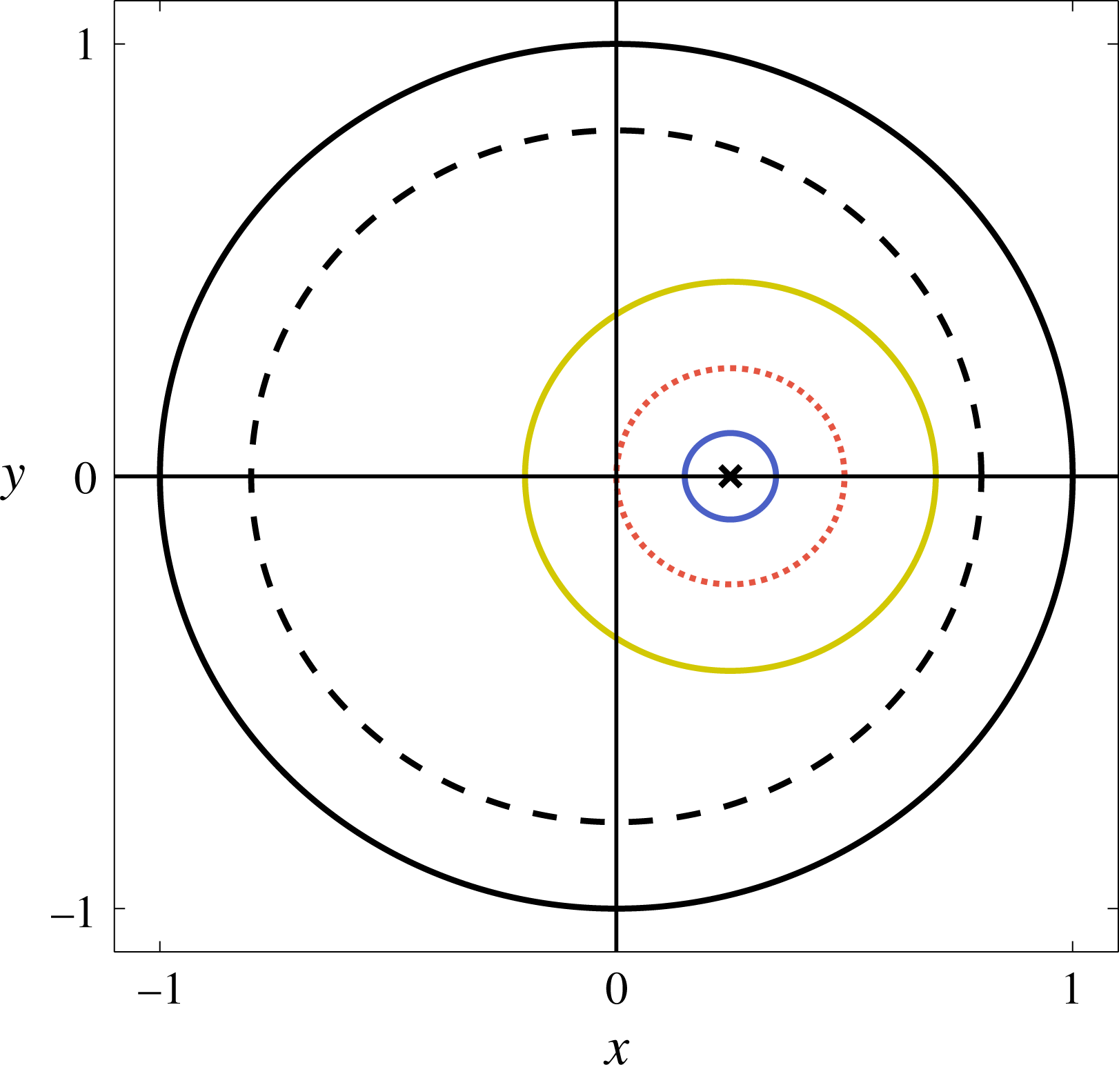
The time derivative becomes
 $$\begin{eqnarray}\frac{\text{d}}{\text{d}t}=\frac{\unicode[STIX]{x2202}}{\unicode[STIX]{x2202}t}+\unicode[STIX]{x1D6FF}\frac{\unicode[STIX]{x2202}}{\unicode[STIX]{x2202}T},\end{eqnarray}$$
and we seek an asymptotic expansion of the form
 $$\begin{eqnarray}\displaystyle & \displaystyle r(t,T)\sim r_{0}(t,T)+\unicode[STIX]{x1D6FF}r_{2}(t,T), & \displaystyle\end{eqnarray}$$
 $$\begin{eqnarray}\displaystyle & \displaystyle \unicode[STIX]{x1D703}(t,T)\sim \unicode[STIX]{x1D703}_{0}(t,T)+\unicode[STIX]{x1D6FF}\unicode[STIX]{x1D703}_{2}(t,T), & \displaystyle\end{eqnarray}$$
 $\unicode[STIX]{x1D6FF}\rightarrow 0$
. We have avoided the subscript
 $1$
in (4.19) for consistency with § 4.3. Substituting (4.19) into (4.17), the
 $O(1)$
terms are
 $$\begin{eqnarray}\displaystyle & \displaystyle r_{0}r_{0t}+\overline{R}(r_{0t}\cos \unicode[STIX]{x1D703}_{0}+r_{0}(1-\unicode[STIX]{x1D703}_{0t})\sin \unicode[STIX]{x1D703}_{0})=0, & \displaystyle\end{eqnarray}$$
 $$\begin{eqnarray}\displaystyle & \displaystyle r_{0}^{2}(1-\unicode[STIX]{x1D703}_{0t})+\overline{R}(r_{0}(1-\unicode[STIX]{x1D703}_{0t})\cos \unicode[STIX]{x1D703}_{0}-r_{0t}\sin \unicode[STIX]{x1D703}_{0})=0, & \displaystyle\end{eqnarray}$$
 $$\begin{eqnarray}r_{0}=r_{0}(T),\quad \unicode[STIX]{x1D703}_{0}=t+\unicode[STIX]{x1D719}(T),\end{eqnarray}$$
and the solutions are
 $2\unicode[STIX]{x03C0}$
-periodic on the short time scale
 $t$
. Thus, the leading-order solutions to the toy and full problems are circular orbits around the steady point (figure 5). Moreover, the construct motion regime over this short time scale is: steady if
 $r(0)=0$
(black cross), settling if
 $r(0)<|\overline{R}|$
(blue), and orbital if
 $r(0)>|\overline{R}|$
(yellow). Additionally, we note that the construct will hit the bioreactor wall if
 $r(0)+|\overline{R}|\geqslant 1-b$
(black dashed). This inequality provides parameter constraints to avoid the construct hitting the bioreactor wall on the fast time scale. Thus, we require
 $r(0)+|\overline{R}|<1-b$
for the construct orbit to be entirely contained within the bioreactor on the fast time scale.
Recalling that
 $\overline{R}=\overline{B}(\bar{\unicode[STIX]{x1D70C}}-1)$
, we may deduce from the inequality above how the values that
 $r(0)$
can take depend on the values of
 $\overline{B}$
and
 $\bar{\unicode[STIX]{x1D70C}}$
, and additionally that the steady point is only within the allowable physical domain when
 $\overline{B}|\bar{\unicode[STIX]{x1D70C}}-1|<1-b$
(figure 6). We further show in figure 6(b) how the construct motion regime depends on
 $r_{0}$
,
 $\overline{B}$
, and
 $\bar{\unicode[STIX]{x1D70C}}$
. As the steady point
 $\overline{R}=\overline{B}(\bar{\unicode[STIX]{x1D70C}}-1)$
increases in magnitude, there are more construct trajectories that will hit the bioreactor edge.
The parameter constraints to keep the construct from hitting the bioreactor edge. The white regions denote valid values and the grey regions denote invalid values. (a)
 $(\bar{\unicode[STIX]{x1D70C}},\overline{B})$
space: the white region is defined by
 $\overline{B}|1-\bar{\unicode[STIX]{x1D70C}}|<1-b$
. (b)
 $(\bar{\unicode[STIX]{x1D70C}},r_{0})$
space: the white region is defined by
 $r_{0}+\overline{B}|1-\bar{\unicode[STIX]{x1D70C}}|<1-b$
. The dotted red lines at
 $r_{0}=\overline{B}|1-\bar{\unicode[STIX]{x1D70C}}|$
define the boundaries between orbital and settling motion regimes, and the dashed blue line at
 $r_{0}=0$
denotes the steady regime.
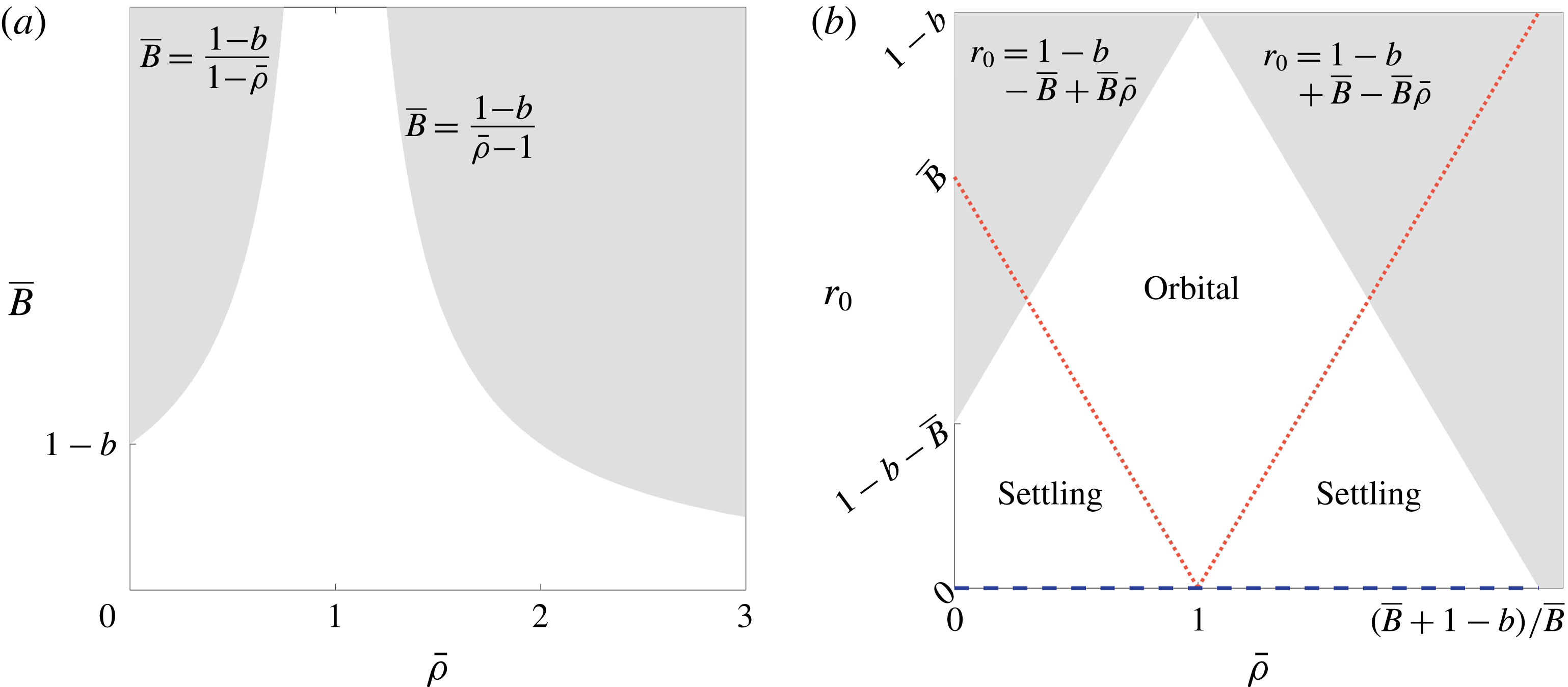
The leading-order results (4.21) simplify the
 $O(\unicode[STIX]{x1D6FF})$
terms in (4.17), which become
 $$\begin{eqnarray}\displaystyle & \displaystyle r_{0}r_{2t}+\overline{R}(r_{2t}\cos \unicode[STIX]{x1D703}_{0}-r_{0}\unicode[STIX]{x1D703}_{2t}\sin \unicode[STIX]{x1D703}_{0})=\unicode[STIX]{x1D707}(r_{0},\unicode[STIX]{x1D703}_{0}), & \displaystyle\end{eqnarray}$$
 $$\begin{eqnarray}\displaystyle & \displaystyle r_{0}^{2}\unicode[STIX]{x1D703}_{2t}+\overline{R}(r_{0}\unicode[STIX]{x1D703}_{2t}\cos \unicode[STIX]{x1D703}_{0}+r_{2t}\sin \unicode[STIX]{x1D703}_{0})=\unicode[STIX]{x1D708}(r_{0},\unicode[STIX]{x1D703}_{0}), & \displaystyle\end{eqnarray}$$
 $$\begin{eqnarray}\displaystyle \unicode[STIX]{x1D707}(r_{0},\unicode[STIX]{x1D703}_{0}) & = & \displaystyle {\displaystyle \frac{\bar{\unicode[STIX]{x1D70C}}}{2}}r_{0}(r_{0}+\overline{R}\cos \unicode[STIX]{x1D703}_{0})-r_{0T}(r_{0}+\overline{R}\cos \unicode[STIX]{x1D703}_{0})+r_{0}\unicode[STIX]{x1D703}_{0T}\overline{R}\sin \unicode[STIX]{x1D703}_{0}\nonumber\\ \displaystyle & & \displaystyle \quad -\,{\displaystyle \frac{(r_{0}(r_{0}+\overline{R}\cos \unicode[STIX]{x1D703}_{0}))^{2}}{2(r_{0}^{2}+2r_{0}\overline{R}\cos \unicode[STIX]{x1D703}_{0}+\overline{R}^{2})}},\end{eqnarray}$$
 $$\begin{eqnarray}\unicode[STIX]{x1D708}(r_{0},\unicode[STIX]{x1D703}_{0})={\displaystyle \frac{\bar{\unicode[STIX]{x1D70C}}}{2}}r_{0}\overline{R}\sin \unicode[STIX]{x1D703}_{0}-r_{0}\unicode[STIX]{x1D703}_{0T}(r_{0}+\overline{R}\cos \unicode[STIX]{x1D703}_{0})-r_{0T}\overline{R}\sin \unicode[STIX]{x1D703}_{0}.\end{eqnarray}$$
To determine equations for
 $r_{0}(T)$
and
 $\unicode[STIX]{x1D719}(T)$
, we need to impose the secularity condition that arises from the assumption that the solution to the system (4.22) is
 $2\unicode[STIX]{x03C0}$
-periodic in
 $t$
. This is equivalent to imposing orthogonality of the solutions of the adjoint problem under periodic boundary conditions via the Fredholm Alternative Theorem. Since this procedure is less well known for systems, we first describe it in abstract terms.
Consider the linear system for a 2D vector function
 $(x_{1},x_{2})$
, as follows
 $$\begin{eqnarray}L(x)=\left(\begin{array}{@{}cc@{}}L_{1} & L_{2}\\ L_{3} & L_{4}\end{array}\right)\left(\begin{array}{@{}c@{}}x_{1}\\ x_{2}\end{array}\right)=\left(\begin{array}{@{}c@{}}f_{1}\\ f_{2}\end{array}\right),\end{eqnarray}$$
where
 $f_{1},f_{2},x_{1},x_{2}$
are functions of
 $t\in (0,2\unicode[STIX]{x03C0})$
,
 $x_{1}$
and
 $x_{2}$
have periodic boundary conditions on
 $t=0$
,
 $2\unicode[STIX]{x03C0}$
, and the
 $L_{i}$
are linear operators. If there is a non-trivial solution of the adjoint problem
 $$\begin{eqnarray}\left(\begin{array}{@{}cc@{}}L_{1}^{\ast } & L_{3}^{\ast }\\ L_{2}^{\ast } & L_{4}^{\ast }\end{array}\right)\left(\begin{array}{@{}c@{}}y_{1}\\ y_{2}\end{array}\right)=\left(\begin{array}{@{}c@{}}0\\ 0\end{array}\right),\end{eqnarray}$$
with periodic boundary conditions, the original problem has solvability condition
 $$\begin{eqnarray}\int _{0}^{2\unicode[STIX]{x03C0}}(y_{1}f_{1}+y_{2}f_{2})\,\text{d}t=0.\end{eqnarray}$$
For the
 $O(\unicode[STIX]{x1D6FF})$
system defined in (4.22), the solvability condition (4.26) is
 $$\begin{eqnarray}\int _{0}^{2\unicode[STIX]{x03C0}}{\displaystyle \frac{(r_{0}+\overline{R}\cos \unicode[STIX]{x1D703}_{0})\unicode[STIX]{x1D707}+\overline{R}\sin \unicode[STIX]{x1D703}_{0}\unicode[STIX]{x1D708}}{\overline{R}^{2}+2r_{0}\overline{R}\cos \unicode[STIX]{x1D703}_{0}+r_{0}^{2}}}\,\text{d}t=0,\quad \int _{0}^{2\unicode[STIX]{x03C0}}{\displaystyle \frac{(r_{0}+\overline{R}\cos \unicode[STIX]{x1D703}_{0})\unicode[STIX]{x1D708}-\overline{R}\sin \unicode[STIX]{x1D703}_{0}\unicode[STIX]{x1D707}}{r_{0}(\overline{R}^{2}+2r_{0}\overline{R}\cos \unicode[STIX]{x1D703}_{0}+r_{0}^{2})}}\,\text{d}t=0.\end{eqnarray}$$
Substituting (4.23) into (4.27) yields the solvability conditions
 $$\begin{eqnarray}\displaystyle & \displaystyle r_{0T}={\displaystyle \frac{\bar{\unicode[STIX]{x1D70C}}}{2}}r_{0}-{\displaystyle \frac{r_{0}^{2}}{4\unicode[STIX]{x03C0}}}\int _{0}^{2\unicode[STIX]{x03C0}}{\displaystyle \frac{(r_{0}+\overline{R}\cos \unicode[STIX]{x1D703}_{0})^{3}}{(r_{0}^{2}+2r_{0}\overline{R}\cos \unicode[STIX]{x1D703}_{0}+\overline{R}^{2})^{2}}}\,\text{d}t, & \displaystyle\end{eqnarray}$$
 $$\begin{eqnarray}\displaystyle & \displaystyle \unicode[STIX]{x1D703}_{0T}={\displaystyle \frac{\overline{R}r_{0}}{4\unicode[STIX]{x03C0}}}\int _{0}^{2\unicode[STIX]{x03C0}}{\displaystyle \frac{\sin \unicode[STIX]{x1D703}_{0}(r_{0}+\overline{R}\cos \unicode[STIX]{x1D703}_{0})^{2}}{(r_{0}^{2}+2r_{0}\overline{R}\cos \unicode[STIX]{x1D703}_{0}+\overline{R}^{2})^{2}}}\,\text{d}t. & \displaystyle\end{eqnarray}$$
 $t=\unicode[STIX]{x03C0}-\unicode[STIX]{x1D703}(0)$
. Therefore, the long-time evolution of the angular velocity is given by
 $$\begin{eqnarray}\unicode[STIX]{x1D703}_{0T}=0,\end{eqnarray}$$
so that
 $\unicode[STIX]{x1D703}_{0}$
is independent of
 $T$
. We evaluate the integral in (4.28a
) using contour integration, obtaining
 $$\begin{eqnarray}\displaystyle \int _{0}^{2\unicode[STIX]{x03C0}}{\displaystyle \frac{(r_{0}+\overline{R}\cos \unicode[STIX]{x1D703}_{0})^{3}\,\text{d}t}{(r_{0}^{2}+2r_{0}\overline{R}\cos \unicode[STIX]{x1D703}_{0}+\overline{R}^{2})^{2}}} & = & \displaystyle \int _{0}^{2\unicode[STIX]{x03C0}}{\displaystyle \frac{(r_{0}+\overline{R}\cos t)^{3}\,\text{d}t}{(r_{0}^{2}+2r_{0}\overline{R}\cos t+\overline{R}^{2})^{2}}}\nonumber\\ \displaystyle & = & \displaystyle \left\{\begin{array}{@{}ll@{}}\displaystyle 0\quad & \displaystyle \text{if }r_{0}<|\overline{R}|,\\ \displaystyle {\displaystyle \frac{\unicode[STIX]{x03C0}}{r_{0}^{3}}}(2r_{0}^{2}-\overline{R}^{2})\quad & \displaystyle \text{if }r_{0}>|\overline{R}|.\end{array}\right.\end{eqnarray}$$
We note that the result depends on whether
 $r_{0}<|\overline{R}|$
or
 $r_{0}>|\overline{R}|$
, i.e. whether the construct is in settling or orbital motion. This is because the integrand in (4.30) stems from the centrifugal force of the fluid acting on the construct (which we introduced as proportional to
 $\dot{\unicode[STIX]{x1D711}}^{2}$
), and the discontinuity of the integral arises because the effect of centrifugal force averaged over one periodic orbit is discontinuous as we move from
 $r_{0}<|\overline{R}|$
(settling) to
 $r_{0}>|\overline{R}|$
(orbital). To get a sense of why this is the case, note that the average of
 $\dot{\unicode[STIX]{x1D711}}$
over one orbit is
 $0$
for settling motion and
 $1$
for orbital motion. Although the introduced centrifugal force has a factor of
 $\dot{\unicode[STIX]{x1D711}}^{2}$
and not
 $\dot{\unicode[STIX]{x1D711}}$
, the discontinuity across motion regimes will transfer from
 $\dot{\unicode[STIX]{x1D711}}$
to
 $\dot{\unicode[STIX]{x1D711}}^{2}$
.
Using the integral result (4.30) in the secularity condition (4.28a ), we obtain the governing equation
 $$\begin{eqnarray}\frac{\text{d}r_{0}}{\text{d}T}=\left\{\begin{array}{@{}ll@{}}\displaystyle {\displaystyle \frac{\bar{\unicode[STIX]{x1D70C}}}{2}}r_{0}\quad & \displaystyle \text{if }r_{0}<|\overline{R}|,\\ \displaystyle {\displaystyle \frac{\bar{\unicode[STIX]{x1D70C}}-1}{2}}r_{0}+{\displaystyle \frac{\overline{R}^{2}}{4r_{0}}}\quad & \displaystyle \text{if }r_{0}>|\overline{R}|.\end{array}\right.\end{eqnarray}$$
As (4.30) is discontinuous at
 $r_{0}=|\overline{R}|$
, (4.31) is also discontinuous at the same point. We note that
 $r_{0T}$
scales linearly with
 $r_{0}$
for
 $r_{0}<|\overline{R}|$
(settling regime). In the orbital regime, when
 $r_{0}>|\overline{R}|$
, we see that
 $r_{0T}$
tends to a linear function of
 $r_{0}$
with gradient
 $(\bar{\unicode[STIX]{x1D70C}}-1)/2$
as
 $r_{0}$
increases, decaying to this function at a decreasing rate.
Though we can solve (4.31) analytically as follows
 $$\begin{eqnarray}r_{0}=\left\{\begin{array}{@{}ll@{}}\displaystyle r_{0}(0)\exp \left({\displaystyle \frac{\bar{\unicode[STIX]{x1D70C}}T}{2}}\right)\quad & \displaystyle \text{if }r_{0}<|\overline{R}|,\\ \displaystyle \left(\left(r_{0}^{2}(0)+{\displaystyle \frac{\overline{R}^{2}}{2(\bar{\unicode[STIX]{x1D70C}}-1)}}\right)\exp ((\bar{\unicode[STIX]{x1D70C}}-1)T)-{\displaystyle \frac{\overline{R}^{2}}{2(\bar{\unicode[STIX]{x1D70C}}-1)}}\right)^{1/2}\quad & \displaystyle \text{if }r_{0}>|\overline{R}|,\end{array}\right.\end{eqnarray}$$
noting that the construct hits the bioreactor wall if
 $r_{0}+|\overline{R}|\geqslant 1-b$
, it is constructive to analyse the long-time behaviour of the system by investigating the sign of the right-hand side of (4.31). This is also the route we take in the full problem, when an analytic solution is not feasible. We consider the system behaviour under the independent variation of
 $\overline{B}$
and
 $\bar{\unicode[STIX]{x1D70C}}$
. These parameters serve as proxies for the independent variation of
 $\unicode[STIX]{x1D6FA}$
and
 $\unicode[STIX]{x1D70C}_{c}$
, the bioreactor angular velocity and the construct density, respectively, which are the main experimentally controllable parameters. We note that
 $\overline{B}$
is inversely proportional to
 $\unicode[STIX]{x1D6FA}$
, and
 $\bar{\unicode[STIX]{x1D70C}}$
is directly proportional to
 $\unicode[STIX]{x1D70C}_{c}$
. As
 $\overline{R}=\overline{B}(\bar{\unicode[STIX]{x1D70C}}-1)$
, we emphasize that a change in either of these experimental parameters will change the steady point of the system. We now discuss the possible long-time behaviours for the toy problem.
Stability and bifurcation diagrams showing the possible long-time behaviours for the toy problem. In the unshaded region, the construct is in one of two general motion behaviours separated by the dotted blue lines, as discussed in the main text. In the shaded regions, the construct hits the bioreactor edge during the first attempted orbit, and our model breaks down. (a) The long-time construct behaviour in
 $(\bar{\unicode[STIX]{x1D70C}},\overline{B})$
parameter space. The shaded regions have boundaries defined by
 $\overline{B}|1-\bar{\unicode[STIX]{x1D70C}}|=1-b$
. (b) A bifurcation diagram of
 $r_{0}$
against
 $\bar{\unicode[STIX]{x1D70C}}$
, for fixed
 $\overline{B}\in ((1-b)/2,1-b)$
. Over the long time,
 $r_{0}$
will vary in the direction of the arrows. The solid black line represents a stable limit cycle and the dashed black line an unstable spiral. The constraints and short-time motion regimes are the same as those in figure 6. That is, the orbital and settling motion regimes are above and below the dotted red line, respectively, which is obscured by the stable limit cycle for behaviour Ia, and the shaded regions have boundaries defined by
 $r_{0}+\overline{B}|1-\bar{\unicode[STIX]{x1D70C}}|=1-b$
.
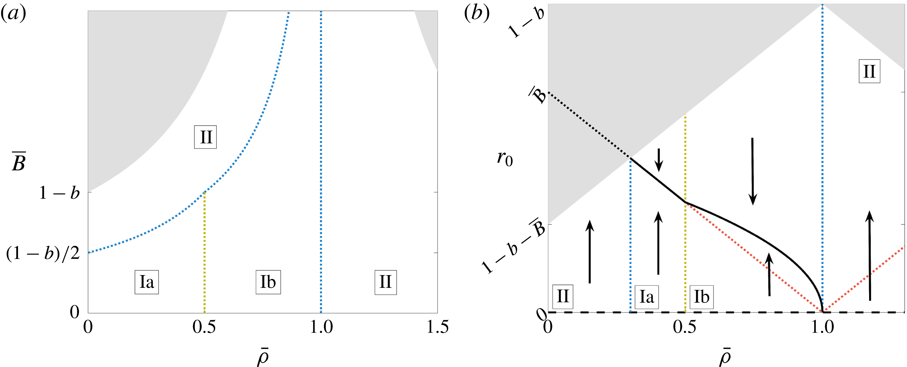
We present the bifurcation results for the toy problem in figure 7 and a schematic of the long-time behaviours within the bioreactor in figure 8. To briefly summarize figure 7 before going into the details, the dotted blue vertical line at
 $\bar{\unicode[STIX]{x1D70C}}=1$
denotes a change in the stability of the steady point at
 $r_{0}=0$
and the death of a stable limit cycle, the dotted yellow vertical line at
 $\bar{\unicode[STIX]{x1D70C}}=0.5$
arises from the location of the stable limit cycle moving fully into the orbital regime from the boundary between settling and orbital motions, and the remaining blue dotted line arises from the stable limit cycle moving outside the bioreactor domain, leading to all trajectories eventually hitting the bioreactor edge. To evaluate the long-time behaviour, it is helpful to first understand the system without the constraint of the construct hitting the bioreactor wall when
 $r_{0}+|\overline{R}|\geqslant 1-b$
. From (4.31) we see that while in settling motion (
 $r_{0}<|\overline{R}|$
), the construct will always spiral out until it reaches the boundary between settling and orbital motion at
 $r_{0}=|\overline{R}|$
in finite time. This boundary is the trajectory that goes through the centre of the bioreactor. Thus, the point
 $r_{0}=0$
is always an unstable spiral. Depending on the parameter values, several things can occur when the construct reaches the boundary between settling and orbital motion, which we now examine.
A schematic of the three possible motion regimes for the toy problem. In Regime Ia, the construct always tends to a stable limit cycle on the boundary between settling and orbital motion. In Regime Ib, the construct always tends to a stable limit cycle in orbital motion. In Regime II, the construct always spirals out until it hits the bioreactor edge. The crosses denote an unstable steady point and the blue solid lines denote a stable limit cycle.
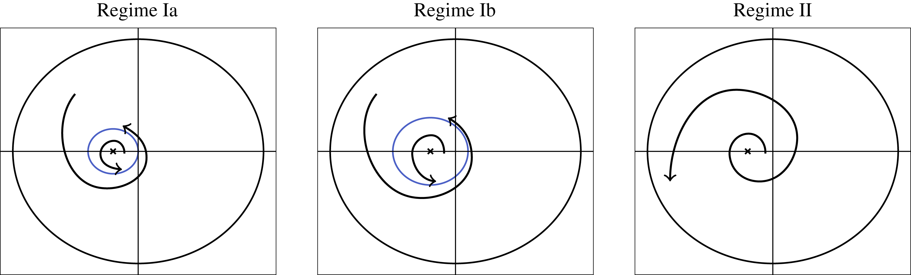
When in orbital motion (
 $r_{0}>|\overline{R}|$
), the long-time construct trajectory depends on the value of
 $\bar{\unicode[STIX]{x1D70C}}$
, and is separated into two main behaviours. If
 $\bar{\unicode[STIX]{x1D70C}}<1$
, the construct will tend to a stable limit cycle (behaviour I in figure 7). If
 $\bar{\unicode[STIX]{x1D70C}}>1$
, the right-hand side of (4.31) is always positive, and therefore the construct will always spiral outwards (behaviour II in figure 7). The location of the stable limit cycle that appears for
 $\bar{\unicode[STIX]{x1D70C}}<1$
depends on the value of
 $\bar{\unicode[STIX]{x1D70C}}$
, and exhibits two sub-behaviours. If
 $\bar{\unicode[STIX]{x1D70C}}<1/2$
, then we see from (4.31) that
 $r_{0T}<0$
for all
 $r_{0}>|\overline{R}|$
. Thus, whether in orbital or settling motion, the construct will always tend towards the orbit which lies on the boundary between these two motion regimes when
 $\bar{\unicode[STIX]{x1D70C}}<1/2$
. We refer to this as behaviour Ia in figure 7. For
 $\bar{\unicode[STIX]{x1D70C}}\in (1/2,1)$
, we see from (4.31) that there is a critical value of
 $r_{0}$
for which
 $r_{0T}=0$
, occurring when
 $$\begin{eqnarray}r_{0}^{c}={\displaystyle \frac{|\overline{R}|}{\sqrt{2(1-\bar{\unicode[STIX]{x1D70C}})}}}=\overline{B}\sqrt{{\displaystyle \frac{1-\bar{\unicode[STIX]{x1D70C}}}{2}}},\end{eqnarray}$$
where we use (4.11) for the second equality in (4.33). As
 $\unicode[STIX]{x2202}r_{0T}/\unicode[STIX]{x2202}r_{0}<0$
at
 $r_{0}=r_{0}^{c}$
(which is always within the orbital regime for
 $\bar{\unicode[STIX]{x1D70C}}\in (1/2,1)$
), this critical value corresponds to a stable limit cycle for the trajectory in the orbital regime. This behaviour is marked as Ib in figure 7.
Thus, there is a bifurcation in the system at
 $\bar{\unicode[STIX]{x1D70C}}=1$
; a stable limit cycle grows out of the bioreactor centre for
 $\bar{\unicode[STIX]{x1D70C}}<1$
, and is annihilated as
 $\bar{\unicode[STIX]{x1D70C}}\rightarrow 1^{-}$
. As the scaling
 $r_{0}\sim \overline{B}$
removes
 $\overline{B}$
from the system (4.31), figure 7(b) is valid for all
 $\overline{B}$
, and the geometrical effect of varying
 $\overline{B}$
in figure 7(b) is to vary the intersections of both the grey boundary and the dotted red line with
 $\bar{\unicode[STIX]{x1D70C}}=0$
.
In this toy problem, the construct can reach the stable limit cycle at the boundary between settling and orbital motion for
 $\bar{\unicode[STIX]{x1D70C}}<1/2$
in finite rather than infinite time. This is because the right-hand side of (4.31), the equation governing the long-time behaviour of the construct, is discontinuous at this boundary. Rather than
 $\text{d}r_{0}/\text{d}T=0$
at
 $r_{0}=|\overline{R}|$
, we instead have
 $\text{d}r_{0}/\text{d}T>0$
for
 $r_{0}\rightarrow |\overline{R}|^{-}$
and
 $\text{d}r_{0}/\text{d}T<0$
for
 $r_{0}\rightarrow |\overline{R}|^{+}$
when
 $\bar{\unicode[STIX]{x1D70C}}<1/2$
.
We now consider the constraint
 $r_{0}+|\overline{R}|<1-b$
, required to keep the construct from hitting the bioreactor wall. More trajectories hit the bioreactor wall when
 $|\overline{R}|=\overline{B}|1-\bar{\unicode[STIX]{x1D70C}}|$
is larger, and this would cause the area of the grey region in figure 7(b) to increase as
 $\overline{B}$
is increased. This corresponds to the steady point moving towards the bioreactor edge, and would eventually cause the stable limit cycle to hit the bioreactor edge. Keeping
 $\bar{\unicode[STIX]{x1D70C}}$
constant, and increasing
 $\overline{B}$
from zero in figure 7(b), we can see when this would occur and quantify the critical parameter relationship. When the boundary of the leftmost grey region (with relationship
 $r_{0}+\overline{B}(1-\bar{\unicode[STIX]{x1D70C}})=1-b$
) intersects the stable limit cycle in Ia (the boundary between settling and orbital motion with relationship
 $r_{0}=\overline{B}(1-\bar{\unicode[STIX]{x1D70C}})$
), the parameter relationship is
 $$\begin{eqnarray}\overline{B}={\displaystyle \frac{1-b}{2(1-\bar{\unicode[STIX]{x1D70C}})}}\quad \text{for }\bar{\unicode[STIX]{x1D70C}}\in (0,1/2),\end{eqnarray}$$
yielding the boundary between Ia and II in figure 7(a). Similarly, the boundary of the leftmost grey region intersects the stable limit cycle in Ib (with relationship (4.33)) when
 $$\begin{eqnarray}\overline{B}={\displaystyle \frac{1-b}{1-\bar{\unicode[STIX]{x1D70C}}+\sqrt{{\displaystyle \frac{1-\bar{\unicode[STIX]{x1D70C}}}{2}}}}}\quad \text{for }\bar{\unicode[STIX]{x1D70C}}\in (1/2,1),\end{eqnarray}$$
yielding the boundary between Ib and II in figure 7(a).
Our toy model suggests that the construct will never remain within the settling regime, because it will instead either tend to the orbital regime or the bioreactor edge in finite time. Further, if
 $\bar{\unicode[STIX]{x1D70C}}>1$
, the construct will hit the bioreactor edge in finite time no matter where it starts. If
 $\bar{\unicode[STIX]{x1D70C}}<1$
, the long-time behaviour will depend on the parameter values of
 $\bar{\unicode[STIX]{x1D70C}}$
,
 $\overline{B}$
, and
 $b$
, either tending to a stable limit cycle or hitting the bioreactor edge, as described in figure 7. Notably, our toy model suggests that drift will always occur in the HARV bioreactor due to weak inertia, and is thus not solely down to cell growth varying the construct density. Additionally, the discontinuity in the long-time ordinary differential equations we derive (4.31), at the boundary between the settling and orbital regimes, suggests that we may encounter a sharp change in construct behaviour between the settling and orbital regimes.
In the next subsection, we analyse the full problem as defined in (4.10) using the method of multiple scales. We then discuss the results and how they compare to the model described in this subsection.
4.3 Full problem
We now analyse (4.10) using the method of multiple scales. As the equilibrium point
 $R=\overline{R}$
remains the same as for the toy problem at leading order, we continue to use the polar coordinate system defined in (4.16) for the full problem. The presence of an
 $O(\unicode[STIX]{x1D716}_{1})$
term in the full equations motivates the introduction of an intermediate time scale
 $\unicode[STIX]{x1D70F}=\unicode[STIX]{x1D716}_{1}t$
, along with the long time scale
 $T=\unicode[STIX]{x1D6FF}t$
used in the previous subsection. The time derivative then becomes
 $$\begin{eqnarray}\frac{\text{d}}{\text{d}t}=\frac{\unicode[STIX]{x2202}}{\unicode[STIX]{x2202}t}+\unicode[STIX]{x1D716}_{1}\frac{\unicode[STIX]{x2202}}{\unicode[STIX]{x2202}\unicode[STIX]{x1D70F}}+\unicode[STIX]{x1D6FF}\frac{\unicode[STIX]{x2202}}{\unicode[STIX]{x2202}T},\end{eqnarray}$$
and we seek asymptotic expansions of the form
 $$\begin{eqnarray}\displaystyle & \displaystyle r(t,\unicode[STIX]{x1D70F},T)\sim r_{0}(t,\unicode[STIX]{x1D70F},T)+\unicode[STIX]{x1D716}_{1}r_{1}(t,\unicode[STIX]{x1D70F},T)+\unicode[STIX]{x1D6FF}r_{2}(t,\unicode[STIX]{x1D70F},T), & \displaystyle\end{eqnarray}$$
 $$\begin{eqnarray}\displaystyle & \displaystyle \unicode[STIX]{x1D703}(t,\unicode[STIX]{x1D70F},T)\sim \unicode[STIX]{x1D703}_{0}(t,\unicode[STIX]{x1D70F},T)+\unicode[STIX]{x1D716}_{1}\unicode[STIX]{x1D703}_{1}(t,\unicode[STIX]{x1D70F},T)+\unicode[STIX]{x1D6FF}\unicode[STIX]{x1D703}_{2}(t,\unicode[STIX]{x1D70F},T), & \displaystyle\end{eqnarray}$$
 $\unicode[STIX]{x1D716}_{1},\unicode[STIX]{x1D6FF}\rightarrow 0$
. Recall that
 $\unicode[STIX]{x1D716}_{1}\ll \unicode[STIX]{x1D716}Re\ll 1$
and, as
 $\unicode[STIX]{x1D6FF}=\unicode[STIX]{x1D716}_{1}\unicode[STIX]{x1D716}Re$
, we have
 $\unicode[STIX]{x1D716}_{1}^{2}\ll \unicode[STIX]{x1D6FF}\ll \unicode[STIX]{x1D716}_{1}\ll 1$
, and we do not have to consider terms of
 $O(\unicode[STIX]{x1D716}_{1}^{2})$
.
At
 $O(1)$
, the governing equations (4.10) yield the same equations as in § 4.2, given by (4.20). Thus, we find that
 $$\begin{eqnarray}r_{0}=r_{0}(\unicode[STIX]{x1D70F},T),\quad \unicode[STIX]{x1D703}_{0}=t+\unicode[STIX]{x1D719}_{0}(\unicode[STIX]{x1D70F},T),\end{eqnarray}$$
and the trajectory for
 $t=O(1)$
is thus circular motion around the steady point, as discussed in § 4.2.
At
 $O(\unicode[STIX]{x1D716}_{1})$
, we find that
 $$\begin{eqnarray}\displaystyle & \displaystyle r_{0}r_{1t}+\overline{R}(r_{1t}\cos \unicode[STIX]{x1D703}_{0}-r_{0}\unicode[STIX]{x1D703}_{1t}\sin \unicode[STIX]{x1D703}_{0})=\unicode[STIX]{x1D707}_{1}(r_{0},\unicode[STIX]{x1D703}_{0}), & \displaystyle\end{eqnarray}$$
 $$\begin{eqnarray}\displaystyle & \displaystyle r_{0}^{2}\unicode[STIX]{x1D703}_{1t}+\overline{R}(r_{0}\unicode[STIX]{x1D703}_{1t}\cos \unicode[STIX]{x1D703}_{0}+r_{1t}\sin \unicode[STIX]{x1D703}_{0})=\unicode[STIX]{x1D708}_{1}(r_{0},\unicode[STIX]{x1D703}_{0}), & \displaystyle\end{eqnarray}$$
 $$\begin{eqnarray}\displaystyle & \displaystyle \unicode[STIX]{x1D707}_{1}(r_{0},\unicode[STIX]{x1D703}_{0})=\unicode[STIX]{x1D6FE}_{1}(R_{0})r_{0}\overline{R}\sin \unicode[STIX]{x1D703}_{0}-r_{0\unicode[STIX]{x1D70F}}(r_{0}+\overline{R}\cos \unicode[STIX]{x1D703}_{0})+\overline{R}r_{0}\unicode[STIX]{x1D703}_{0\unicode[STIX]{x1D70F}}\sin \unicode[STIX]{x1D703}_{0}, & \displaystyle\end{eqnarray}$$
 $$\begin{eqnarray}\displaystyle & \displaystyle \unicode[STIX]{x1D708}_{1}(r_{0},\unicode[STIX]{x1D703}_{0})=\unicode[STIX]{x1D6FE}_{1}(R_{0})\overline{R}(\overline{R}+r_{0}\cos \unicode[STIX]{x1D703}_{0})-r_{0}\unicode[STIX]{x1D703}_{0\unicode[STIX]{x1D70F}}(r_{0}+\overline{R}\cos \unicode[STIX]{x1D703}_{0})-r_{0\unicode[STIX]{x1D70F}}\overline{R}\sin \unicode[STIX]{x1D703}_{0},\qquad & \displaystyle\end{eqnarray}$$
 $$\begin{eqnarray}R_{0}(t,\unicode[STIX]{x1D70F},T)=\sqrt{\overline{R}^{2}+2r_{0}(\unicode[STIX]{x1D70F},T)\overline{R}\cos \unicode[STIX]{x1D703}_{0}(t,\unicode[STIX]{x1D70F},T)+r_{0}^{2}(\unicode[STIX]{x1D70F},T)}.\end{eqnarray}$$
We note that the linear operators acting on
 $r_{1}$
and
 $\unicode[STIX]{x1D703}_{1}$
in (4.38) are the same as for those acting on
 $r_{2}$
and
 $\unicode[STIX]{x1D703}_{2}$
in the toy problem in the previous subsection. Thus, the solvability conditions at this order can be obtained by substituting
 $\unicode[STIX]{x1D707}_{1}$
and
 $\unicode[STIX]{x1D708}_{1}$
from (4.39) into (4.27) in place of their unsubscripted counterparts. This yields
 $$\begin{eqnarray}\displaystyle & \displaystyle 0=\int _{0}^{2\unicode[STIX]{x03C0}}(-r_{0\unicode[STIX]{x1D70F}}+\overline{R}\unicode[STIX]{x1D6FE}_{1}(R_{0})\sin \unicode[STIX]{x1D703}_{0})\,\text{d}t, & \displaystyle\end{eqnarray}$$
 $$\begin{eqnarray}\displaystyle & \displaystyle 0=\int _{0}^{2\unicode[STIX]{x03C0}}(-r_{0}\unicode[STIX]{x1D703}_{0\unicode[STIX]{x1D70F}}+\overline{R}\unicode[STIX]{x1D6FE}_{1}(R_{0})\cos \unicode[STIX]{x1D703}_{0})\,\text{d}t. & \displaystyle\end{eqnarray}$$
 $t=\unicode[STIX]{x03C0}+\unicode[STIX]{x1D719}_{0}(\unicode[STIX]{x1D70F},T)$
, and hence does not contribute to the integral. Therefore, we deduce that
 $$\begin{eqnarray}r_{0}=r_{0}(T),\quad r_{0}\frac{\unicode[STIX]{x2202}\unicode[STIX]{x1D719}_{0}}{\unicode[STIX]{x2202}\unicode[STIX]{x1D70F}}={\displaystyle \frac{\overline{R}}{2\unicode[STIX]{x03C0}}}\int _{0}^{2\unicode[STIX]{x03C0}}\unicode[STIX]{x1D6FE}_{1}(R_{0})\cos \unicode[STIX]{x1D703}_{0}\,\text{d}t.\end{eqnarray}$$
Hence, as deduced in § 4.1, there is no drift at
 $t=O(1/\unicode[STIX]{x1D716}_{1})$
. There is, however, a change in the angular velocity of the construct centre around the steady point. Furthermore, using (4.40) we note that
 $R_{0}$
is
 $2\unicode[STIX]{x03C0}$
-periodic in
 $t$
with the same phase as
 $\cos \unicode[STIX]{x1D703}_{0}$
, and using (4.6b
) we note that
 $\unicode[STIX]{x1D6FE}_{1}(R_{0})>0$
is a monotonically increasing function of
 $R_{0}$
. Making the integral substitution
 $u=\cos t$
, we thus determine that the integral in (4.42b
) is always positive. Hence, we deduce that
 $\unicode[STIX]{x2202}\unicode[STIX]{x1D719}_{0}/\unicode[STIX]{x2202}\unicode[STIX]{x1D70F}$
has the same sign as
 $\overline{R}$
, and vanishes when
 $\overline{R}=0$
.
At
 $O(\unicode[STIX]{x1D6FF})$
, the governing equations (4.10) give
 $$\begin{eqnarray}\displaystyle & \displaystyle r_{0}r_{2t}+\overline{R}(r_{2t}\cos \unicode[STIX]{x1D703}_{0}-r_{0}\unicode[STIX]{x1D703}_{2t}\sin \unicode[STIX]{x1D703}_{0})=\unicode[STIX]{x1D707}_{2}(r_{0},\unicode[STIX]{x1D703}_{0}), & \displaystyle\end{eqnarray}$$
 $$\begin{eqnarray}\displaystyle & \displaystyle r_{0}^{2}\unicode[STIX]{x1D703}_{2t}+\overline{R}(r_{0}\unicode[STIX]{x1D703}_{2t}\cos \unicode[STIX]{x1D703}_{0}+r_{2t}\sin \unicode[STIX]{x1D703}_{0})=\unicode[STIX]{x1D708}_{2}(r_{0},\unicode[STIX]{x1D703}_{0}), & \displaystyle\end{eqnarray}$$
 $$\begin{eqnarray}\displaystyle & \displaystyle \unicode[STIX]{x1D707}_{2}(r_{0},\unicode[STIX]{x1D703}_{0})=R_{0}(\unicode[STIX]{x1D6FE}_{2}-\unicode[STIX]{x1D6FE}_{4})+\left({\displaystyle \frac{\bar{\unicode[STIX]{x1D70C}}}{2}}r_{0}-r_{0T}\right)(r_{0}+\overline{R}\cos \unicode[STIX]{x1D703}_{0})+r_{0}\unicode[STIX]{x1D703}_{0T}\overline{R}\sin \unicode[STIX]{x1D703}_{0}, & \displaystyle\end{eqnarray}$$
 $$\begin{eqnarray}\displaystyle & \displaystyle \unicode[STIX]{x1D708}_{2}(r_{0},\unicode[STIX]{x1D703}_{0})=R_{0}(\unicode[STIX]{x1D6FE}_{3}+\unicode[STIX]{x1D6FE}_{5})+\left({\displaystyle \frac{\bar{\unicode[STIX]{x1D70C}}}{2}}r_{0}-r_{0T}\right)\overline{R}\sin \unicode[STIX]{x1D703}_{0}-r_{0}\unicode[STIX]{x1D703}_{0T}\left(r_{0}+\overline{R}\cos \unicode[STIX]{x1D703}_{0}\right).\qquad & \displaystyle\end{eqnarray}$$
As we expect, the linear operators acting on
 $r_{2}$
and
 $\unicode[STIX]{x1D703}_{2}$
in (4.43) are the same as those in the previous subsection. Thus, the solvability conditions can be obtained by substituting
 $\unicode[STIX]{x1D707}_{2}$
and
 $\unicode[STIX]{x1D708}_{2}$
into (4.27) in place of their unsubscripted counterparts, to yield
 $$\begin{eqnarray}\displaystyle & \displaystyle r_{0T}-{\displaystyle \frac{\bar{\unicode[STIX]{x1D70C}}}{2}}r_{0}={\displaystyle \frac{1}{2\unicode[STIX]{x03C0}}}\int _{0}^{2\unicode[STIX]{x03C0}}{\displaystyle \frac{(\unicode[STIX]{x1D6FE}_{2}-\unicode[STIX]{x1D6FE}_{4})(r_{0}+\overline{R}\cos \unicode[STIX]{x1D703}_{0})+(\unicode[STIX]{x1D6FE}_{3}+\unicode[STIX]{x1D6FE}_{5})\overline{R}\sin \unicode[STIX]{x1D703}_{0}}{R_{0}}}\,\text{d}t, & \displaystyle\end{eqnarray}$$
 $$\begin{eqnarray}\displaystyle & \displaystyle r_{0}\unicode[STIX]{x1D703}_{0T}={\displaystyle \frac{1}{2\unicode[STIX]{x03C0}}}\int _{0}^{2\unicode[STIX]{x03C0}}{\displaystyle \frac{(\unicode[STIX]{x1D6FE}_{4}-\unicode[STIX]{x1D6FE}_{2})\overline{R}\sin \unicode[STIX]{x1D703}_{0}+(\unicode[STIX]{x1D6FE}_{5}+\unicode[STIX]{x1D6FE}_{3})(r_{0}+\overline{R}\cos \unicode[STIX]{x1D703}_{0})}{R_{0}}}\,\text{d}t, & \displaystyle\end{eqnarray}$$
 $\unicode[STIX]{x1D6FE}_{2}$
and
 $\unicode[STIX]{x1D6FE}_{3}$
are defined in (4.8b,c
), and the functions
 $\unicode[STIX]{x1D6FE}_{4}$
and
 $\unicode[STIX]{x1D6FE}_{5}$
are defined in (4.9). Each of these are functions of
 $R$
and
 $\unicode[STIX]{x1D711}$
, and thus from (4.16) they are functions of
 $r$
and
 $\unicode[STIX]{x1D703}$
. We can expand these functions using (4.36), yielding solvability conditions for
 $r_{0}$
and
 $\unicode[STIX]{x1D703}_{0}$
.
Of the two solvability conditions in (4.45), we are most interested in (4.45a ), as this condition determines whether the construct spirals inwards or outwards. To facilitate discussion of our results, we rewrite (4.45a ) as
 $$\begin{eqnarray}r_{0T}={\displaystyle \frac{\bar{\unicode[STIX]{x1D70C}}}{2}}r_{0}+{\mathcal{I}},\end{eqnarray}$$
where
 ${\mathcal{I}}={\mathcal{I}}_{p}^{x}+{\mathcal{I}}_{p}^{y}+{\mathcal{I}}_{s}^{x}+{\mathcal{I}}_{s}^{y}$
and
 $$\begin{eqnarray}\left.\begin{array}{@{}c@{}}\displaystyle {\mathcal{I}}_{p}^{x}={\displaystyle \frac{1}{2\unicode[STIX]{x03C0}}}\int _{0}^{2\unicode[STIX]{x03C0}}{\displaystyle \frac{\unicode[STIX]{x1D6FE}_{2}(r_{0}+\overline{R}\cos \unicode[STIX]{x1D703}_{0})}{R_{0}}}\,\text{d}t,\quad {\mathcal{I}}_{p}^{y}={\displaystyle \frac{1}{2\unicode[STIX]{x03C0}}}\int _{0}^{2\unicode[STIX]{x03C0}}{\displaystyle \frac{\unicode[STIX]{x1D6FE}_{3}\overline{R}\sin \unicode[STIX]{x1D703}_{0}}{R_{0}}}\,\text{d}t,\\ \displaystyle {\mathcal{I}}_{s}^{x}=-{\displaystyle \frac{1}{2\unicode[STIX]{x03C0}}}\int _{0}^{2\unicode[STIX]{x03C0}}{\displaystyle \frac{\unicode[STIX]{x1D6FE}_{4}\overline{R}\sin \unicode[STIX]{x1D703}_{0}}{R_{0}}}\,\text{d}t,\quad {\mathcal{I}}_{s}^{y}={\displaystyle \frac{1}{2\unicode[STIX]{x03C0}}}\int _{0}^{2\unicode[STIX]{x03C0}}{\displaystyle \frac{\unicode[STIX]{x1D6FE}_{5}(r_{0}+\overline{R}\cos \unicode[STIX]{x1D703}_{0})}{R_{0}}}\,\text{d}t.\end{array}\right\}\end{eqnarray}$$
We note that
 ${\mathcal{I}}_{p}^{x}$
and
 ${\mathcal{I}}_{p}^{y}$
arise from the first correction to pressure acting on the construct interface in the
 $\boldsymbol{e}_{X}$
and
 $\boldsymbol{e}_{Y}$
directions, respectively, and
 ${\mathcal{I}}_{s}^{x}$
and
 ${\mathcal{I}}_{s}^{y}$
arise from the shear stress acting on the construct interface in the
 $\boldsymbol{e}_{X}$
and
 $\boldsymbol{e}_{Y}$
directions, respectively. We solve (4.46) numerically in the next subsection to efficiently determine the long-time behaviour of the construct.
4.3.1 Evaluating the long-time drift
We determine the long-time behaviour of the construct by evaluating the solvability condition (4.46) to determine
 $\text{d}r_{0}/\text{d}T$
. The right-hand sides of (4.46b
) are numerically evaluated using the trapezium rule. To do this, we must evaluate the infinite sums
 $\unicode[STIX]{x1D6FE}_{2}$
and
 $\unicode[STIX]{x1D6FE}_{3}$
, defined in (4.8b,c
), and the integrals
 $\unicode[STIX]{x1D6FE}_{4}$
and
 $\unicode[STIX]{x1D6FE}_{5}$
, defined in (4.9).
The functions
 $\unicode[STIX]{x1D6FE}_{2}$
and
 $\unicode[STIX]{x1D6FE}_{3}$
arise from the first correction to the fluid pressure acting on the construct interface. They are obtained by determining
 $\overline{E}_{n}$
and
 $\overline{F}_{n}$
, from (3.20e
) and (3.20f
), respectively. This requires the knowledge of
 $a_{in}$
and
 $b_{in}$
(where
 $i\in \{1,2,3\}$
) obtained by equating (3.16) and (3.17). These coefficients can be determined numerically from the calculation of
 $p_{0}$
, given in (3.12a
), and the functions
 $\unicode[STIX]{x1D6F1}$
,
 $\unicode[STIX]{x1D6EC}_{a}$
, and
 $\unicode[STIX]{x1D6EC}_{b}$
we derive in appendix A to couple the outer regions. These last three functions are calculated beforehand for a range of arguments, and then we use numerical interpolation to evaluate each function at the parameter value we require. The functions
 $\unicode[STIX]{x1D6FE}_{4}$
and
 $\unicode[STIX]{x1D6FE}_{5}$
arise from the bulk fluid shear acting on the construct interface. They are obtained by substituting (4.4), the leading-order result for the bulk flow relative to the construct movement, into the shear results given in (4.9), using (3.12a
) to evaluate
 $p_{0}$
. To calculate these functions, we use 10 modes to approximate each infinite series, which suffices since each term is exponentially smaller than the last. We increase this to 40 modes when evaluating an orbit where the construct passes within 0.2 of the bioreactor edge, near which the convergence is slower. We use 100 points to discretize
 $\unicode[STIX]{x1D6FD}\in [0,2\unicode[STIX]{x03C0}]$
and 100 points to discretize
 $t\in [0,2\unicode[STIX]{x03C0}]$
and evaluate (4.46). This is enough because the system is periodic in both
 $\unicode[STIX]{x1D6FD}$
and
 $t$
, providing fast convergence. We checked that there were enough modes in the infinite sums and points in the grid by observing no notable change in the results when each was increased.
We first discuss the behaviour of
 ${\mathcal{I}}$
, which is fundamental to understanding the long-time behaviour of the system. Then, we investigate how our system behaves in terms of experimentally controllable parameters. As predicted by the toy model in § 4.2, there is a sharp change in behaviour as a construct passes between settling and orbital motion (figure 9). The general trend is for
 ${\mathcal{I}}$
to increase at an approximately linear rate with
 $r_{0}$
in the settling regime, then to decay at a decreasing rate as
 $r_{0}$
increases in the orbital regime (figure 9
a). This behaviour is qualitatively the same as that in the toy problem, but without the discontinuities we saw previously. Additionally, we see from figure 9(a) that the main contribution to
 ${\mathcal{I}}$
is from the first-order correction to pressure (
 ${\mathcal{I}}_{p}^{x}$
and
 ${\mathcal{I}}_{p}^{y}$
) rather than the shear stress acting on the construct interface (
 ${\mathcal{I}}_{s}^{x}$
and
 ${\mathcal{I}}_{s}^{y}$
), even though both terms arise at the same asymptotic order. This does not mean that the shear stress acting on the construct at a given point in time is negligible at this order, rather that the average effect of shear stress over one orbit is negligible compared to the average effect of fluid pressure over one orbit.
Although
 ${\mathcal{I}}<0$
for some values of
 $r_{0}$
in figure 9(a), we can never have
 $r_{0T}<0$
for the parameter values used in figure 9. This is because choosing
 $\overline{R}=\overline{B}(\bar{\unicode[STIX]{x1D70C}}-1)>0$
implies that
 $\bar{\unicode[STIX]{x1D70C}}>1$
, and thus the
 $\bar{\unicode[STIX]{x1D70C}}r_{0}/2$
term in (4.46) must be larger than
 $r_{0}/2$
, which is larger than the magnitude of the negative values of
 ${\mathcal{I}}$
. We see that
 $r_{0T}$
is positive in figure 9(b) for a variety of values of
 $\bar{\unicode[STIX]{x1D70C}}$
. This is true in general, and thus our model suggests that a construct that is heavier than the surrounding fluid will always spiral out until it hits the bioreactor edge. However, we will show that if the solid part of the construct is made from material that is lighter than the surrounding fluid, stable limit cycles may exist within the bioreactor.
(a) The function
 ${\mathcal{I}}$
, defined in (4.46), and its component parts. We see that
 ${\mathcal{I}}$
, and hence the contribution to the long-time drift, has a marked change in behaviour at the boundary between these two regions. (b) The value of
 $\text{d}r_{0}/\text{d}T$
, defined in (4.46), using
 ${\mathcal{I}}$
from (a), and
 $\bar{\unicode[STIX]{x1D70C}}=1.01,1.1,1.2,1.3,1.4,1.5$
. Additionally, the boundary between the settling and orbital regimes is denoted by a black dotted line, with settling on the left and orbital motion on the right. For each subfigure, we use parameter values
 $\overline{R}=0.2$
,
 $b=0.2$
, and
 $K=0.05$
.
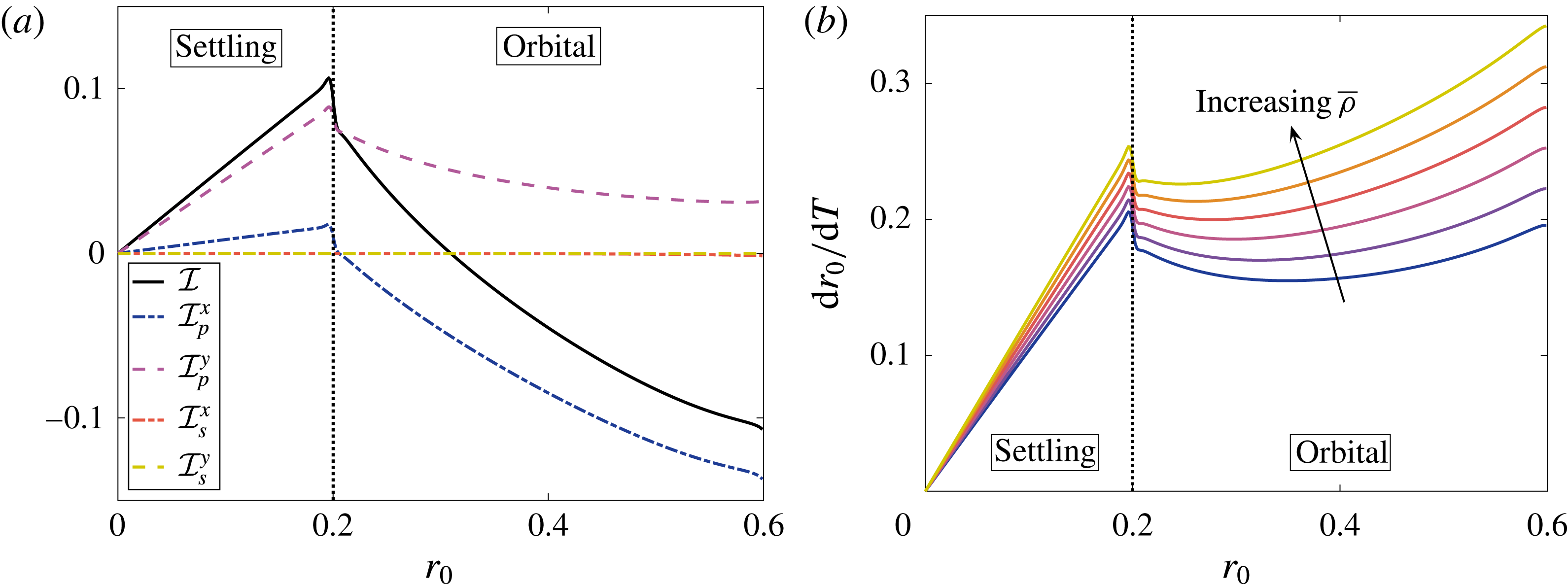
Henceforth, we consider the system behaviour under the independent variation of
 $\overline{B}$
and
 $\bar{\unicode[STIX]{x1D70C}}$
, as for the toy problem. We recall that these parameters serve as proxies for the independent variation of the main experimentally controllable parameters
 $\unicode[STIX]{x1D6FA}$
and
 $\unicode[STIX]{x1D70C}_{c}$
, the bioreactor angular velocity and the construct density, respectively. Again,
 $\overline{B}$
is inversely proportional to
 $\unicode[STIX]{x1D6FA}$
,
 $\bar{\unicode[STIX]{x1D70C}}$
is directly proportional to
 $\unicode[STIX]{x1D70C}_{c}$
, and a change in either of these experimental parameters will change the steady point of the system, since
 $\overline{R}=\overline{B}(\bar{\unicode[STIX]{x1D70C}}-1)$
.
Stability and bifurcation diagrams showing the three possible long-time behaviours (separated by the dotted blue lines) for the full problem, as discussed in the main text. (a) The long-time construct behaviour in
 $(\bar{\unicode[STIX]{x1D70C}},\overline{B})$
parameter space. (b) A bifurcation diagram of
 $r_{0}$
against
 $\bar{\unicode[STIX]{x1D70C}}$
, for
 $\overline{B}=0.1$
. Over the long time scale,
 $r_{0}$
will vary in the direction of the arrows. The solid black line represents a stable limit cycle, the dashed black line represents an unstable spiral, and the dash-dotted line represents an unstable limit cycle. The orbital and settling motion regimes are above and below the dotted red line, respectively. The shaded region has boundary defined by
 $r_{0}+\overline{B}|1-\bar{\unicode[STIX]{x1D70C}}|=1-b$
and represents the construct trajectory hitting the bioreactor edge on the first orbit. We use
 $b=0.2$
and
 $K=0.05$
.
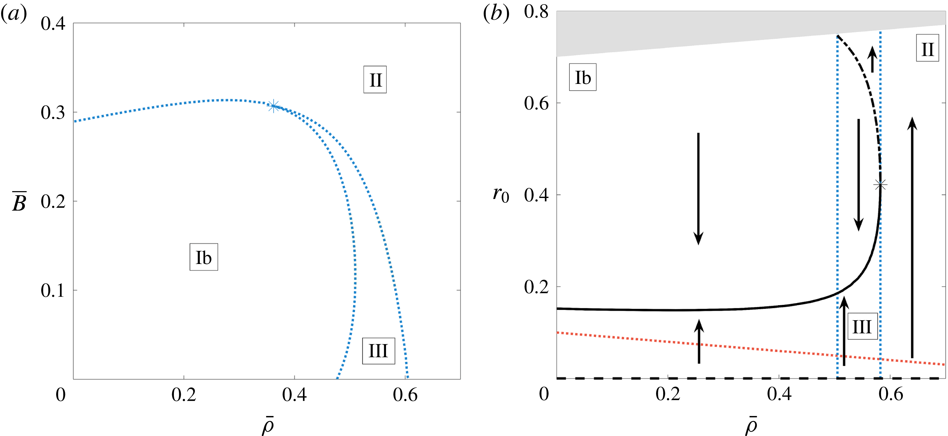
A schematic of the three possible motion regimes for the full problem. In Regime Ib, the construct always tends to a stable limit cycle in orbital motion. In Regime II, the construct always spirals out until it hits the bioreactor edge. In Regime III, there exists both a stable and an unstable limit cycle, so the construct will either tend to the stable limit cycle or spiral out until it hits the bioreactor edge, depending on its initial position. The crosses denote an unstable steady point, the blue solid lines denote a stable limit cycle and the dash-dotted red lines denote an unstable limit cycle.
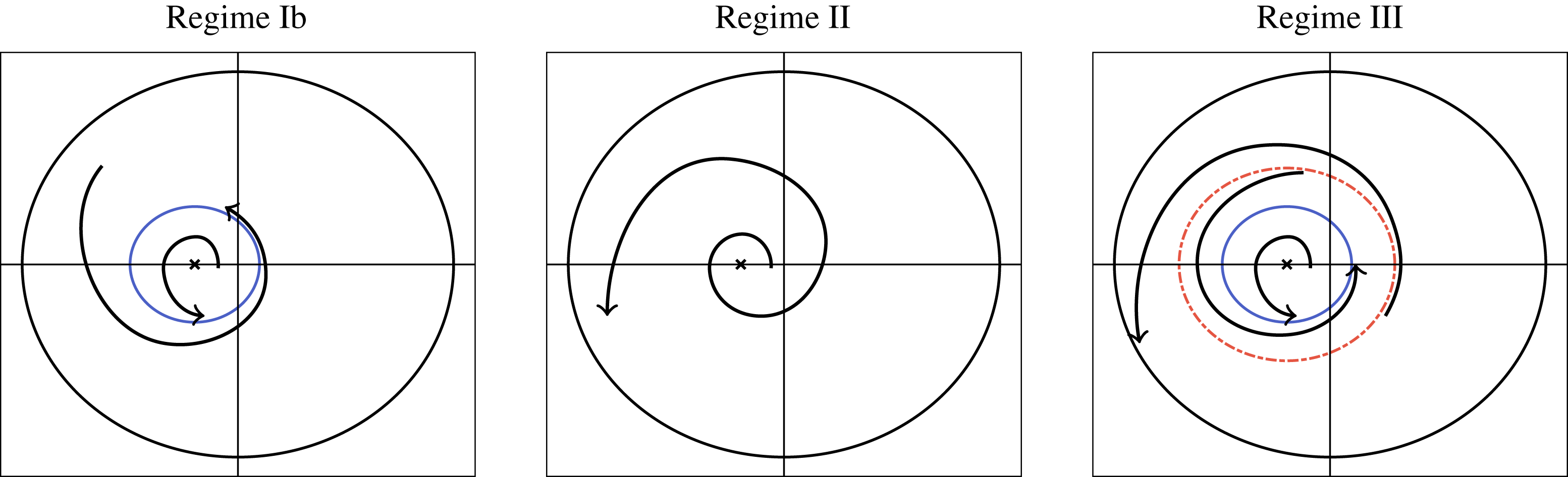
Calculating (4.46) as described above, we find that there are three main long-time behaviours in this system (figures 10 and 11). The first two behaviours are similar to those found in the toy problem, behaviours Ib and II. For
 $\overline{B}$
and
 $\bar{\unicode[STIX]{x1D70C}}$
small enough, there is a stable limit cycle in the system which attracts all initial positions (behaviour Ib in the toy problem). For larger
 $\overline{B}$
and
 $\bar{\unicode[STIX]{x1D70C}}$
, the construct will always spiral out towards the bioreactor edge, in this case the only steady point in the system is
 $r_{0}=0$
, which is always unstable (behaviour II in the toy problem). The final possible behaviour is new to the full system, and thus we define this as behaviour III. In this case, there are both unstable and stable limit cycles in the system (in addition to the ever-present unstable point at
 $r_{0}=0$
), so the long-time behaviour of the system depends strongly on the initial conditions. The transition from behaviours II to III is a saddle–node (or fold) bifurcation of cycles (Strogatz Reference Strogatz2014). That is, the unstable and stable limit cycles appear in the system apropos of nothing, and the stability of the origin is unchanged. The transition from behaviours III to Ib is due to the unstable cycle falling off the physical domain.
We now consider the limit of a quickly rotating bioreactor in more detail. This will allow us to obtain some asymptotic results for the system, such as an analytic result for the parameter values at which the system stability changes. A quickly rotating bioreactor corresponds to
 $\overline{B}\rightarrow 0$
and thus
 $\overline{R}\rightarrow 0$
, from which we additionally attain
 $\dot{R}_{0}\rightarrow 0$
, and
 $\dot{\unicode[STIX]{x1D711}}_{0}\rightarrow 1$
. Thus the construct orbits the bioreactor centre with
 $R_{0}=r_{0}$
in this limit, and the system is in near rigid-body rotation with no flow across the construct interface relative to the construct motion. From these limiting behaviours, we find that all terms in the coupling conditions (3.16) vanish, apart from the
 $-(X^{2}+Y^{2})/2$
term in (3.16b
). It is a simple task to turn this remaining term into a Fourier series in
 $\unicode[STIX]{x1D6FD}$
on the construct interface, and subsequently determine
 $$\begin{eqnarray}\unicode[STIX]{x1D6FE}_{2}=-2R_{0}\sinh ^{2}\unicode[STIX]{x1D6FC}_{2}\mathop{\sum }_{n=1}^{\infty }{\displaystyle \frac{n\tanh n(\unicode[STIX]{x1D6FC}_{2}-\unicode[STIX]{x1D6FC}_{1})\text{e}^{-2n\unicode[STIX]{x1D6FC}_{2}}}{\tanh n(\unicode[STIX]{x1D6FC}_{2}-\unicode[STIX]{x1D6FC}_{1})+12K}},\quad \unicode[STIX]{x1D6FE}_{3}=0,\quad \unicode[STIX]{x1D6FE}_{4}=0,\quad \unicode[STIX]{x1D6FE}_{5}=0.\end{eqnarray}$$
Comparison of numerical and asymptotic results for
 $b=0.2$
and
 $K=0.05$
in the asymptotic limit of
 $\overline{B}\rightarrow 0$
. (a) The solid grey line is
 ${\mathcal{I}}$
, obtained by resolving the solvability condition (4.46) using quadrature. The dashed black line in the asymptotic result (4.49) for
 ${\mathcal{I}}$
for small
 $R_{0}$
. (b) A stability diagram, showing the three possible behaviours of the construct for varying
 $\bar{\unicode[STIX]{x1D70C}}$
. The boundaries between behaviours are denoted with dotted blue lines, and the line
 $\bar{\unicode[STIX]{x1D70C}}=\bar{\unicode[STIX]{x1D70C}}^{\ast }$
(
 ${\approx}0.606$
for the parameter values used in this figure), is obtained using the asymptotic result (4.50) for small
 $R_{0}$
. The solid black line represents a stable spiral, the dashed black line represents an unstable spiral, and the dash-dotted line represents an unstable limit cycle. Over the long time scale,
 $R_{0}$
will vary as discussed in the main text, and the arrows denote the direction of change in
 $R_{0}$
.
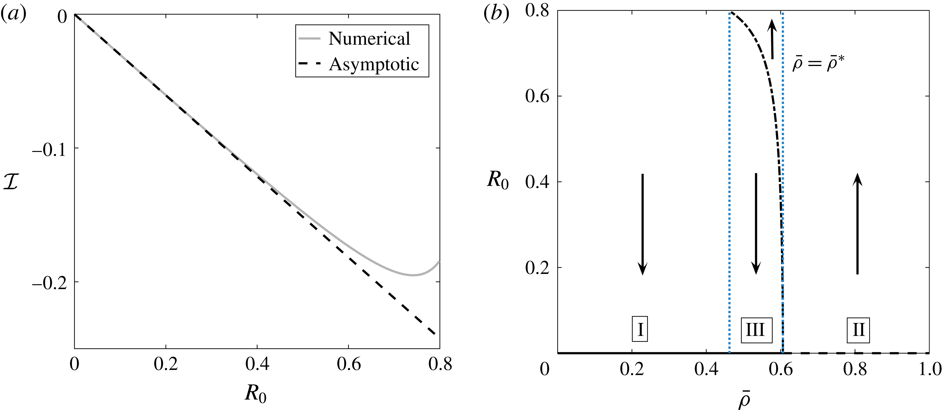
In the further limit of
 $R_{0}\rightarrow 0$
, we use the small
 $R_{0}$
results in appendix B to deduce that
 $$\begin{eqnarray}\unicode[STIX]{x1D6FE}_{2}\sim -{\displaystyle \frac{R_{0}}{2\displaystyle \left(1+12K\left({\displaystyle \frac{1+b^{2}}{1-b^{2}}}\right)\right)}}+O(R_{0}^{3}).\end{eqnarray}$$
Hence, using
 $r_{0}=R_{0}$
, we obtain the asymptotic result
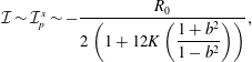 $$\begin{eqnarray}{\mathcal{I}}\sim {\mathcal{I}}_{p}^{x}\sim -{\displaystyle \frac{R_{0}}{2\displaystyle \left(1+12K\left({\displaystyle \frac{1+b^{2}}{1-b^{2}}}\right)\right)}},\end{eqnarray}$$
which shows excellent agreement with the numerical resolution of
 ${\mathcal{I}}$
for
 $\overline{R}=0$
(figure 12
a). Substituting (4.49) into (4.46), we obtain
 $$\begin{eqnarray}{\displaystyle \frac{\text{d}R_{0}}{\text{d}T}}=(\bar{\unicode[STIX]{x1D70C}}-\bar{\unicode[STIX]{x1D70C}}^{\ast }){\displaystyle \frac{R_{0}}{2}}+O(R_{0}^{3})\quad \text{as }R_{0}\rightarrow 0,\end{eqnarray}$$
where
 $$\begin{eqnarray}\bar{\unicode[STIX]{x1D70C}}^{\ast }={\displaystyle \frac{1}{1+12K\displaystyle \left({\displaystyle \frac{1+b^{2}}{1-b^{2}}}\right)}}.\end{eqnarray}$$
Thus, the bifurcation occurs when
 $\bar{\unicode[STIX]{x1D70C}}$
passes through
 $\bar{\unicode[STIX]{x1D70C}}^{\ast }$
, as we see in figure 12(b). As
 $\bar{\unicode[STIX]{x1D70C}}$
decreases through
 $\bar{\unicode[STIX]{x1D70C}}^{\ast }$
,
 $R_{0}=0$
changes from an unstable to a stable spiral, and an unstable limit cycle shoots out. Hence, there is a subcritical Hopf bifurcation at this point. We note that, in the limit
 $\overline{B}\rightarrow 0$
, the settling regime is annihilated, and the stable limit cycle in the orbital regime tends to and coalesces with the steady point at the origin. This explains why we have a Hopf bifurcation instead of a saddle–node bifurcation of cycles when
 $\overline{B}=0$
. As there is no settling regime in this limit, we do not delineate between behaviours Ia and Ib, and we refer to the behaviour where the construct tends to a steady point within the domain as behaviour I. Our asymptotic result (4.50) can also be used to determine where the boundary between behaviours II and III occurs for small
 $\overline{B}$
. As
 $\bar{\unicode[STIX]{x1D70C}}$
is decreased, the first limit cycles appear when
 $\overline{B}=0$
(see figure 10
a). Thus, (4.50b
) also provides a supremum for the values of
 $\bar{\unicode[STIX]{x1D70C}}$
for which stable limit cycles are possible.
Therefore, we conclude that the two possible long-time behaviours of the construct are to spiral out to the bioreactor edge, or towards a stable limit cycle within the bioreactor. In general, stable limit cycles can only exist when the bioreactor is rotating quickly and the tissue construct is lighter than the surrounding fluid. We are able to quantify when each of these behaviours is possible as a function of the system parameters and, moreover, we are able to quantify when the long-time behaviour of the construct depends on its initial position. Moreover, our work shows that spiralling can occur due to weak inertia and no cell growth over a time scale of
 $t=O((\unicode[STIX]{x1D716}_{1}\unicode[STIX]{x1D716}Re)^{-1})$
, and therefore construct spiralling may not be solely due to tissue growth as hypothesized by experimentalists. Using experimental parameters, the time scale of drift due to inertia is on the order of hours, a similar time scale as for tissue growth.
5 Discussion
We investigated the coupled flow and construct motion problem for a saturated porous tissue construct within a fluid-filled rotating high-aspect-ratio vessel bioreactor under the effect of weak inertia. We found that inertia can cause the construct to spiral out towards the bioreactor edge, or to a stable limit cycle within the bioreactor, depending on the system parameters. Notably, we determined that stable limit cycles are only possible when the construct density is less than the fluid density and when the bioreactor is rotating quickly, and we were able to quantify these sentiments by efficiently sweeping through parameter space. We used a combination of asymptotic and numerical methods to solve this nonlinear moving-boundary problem. Our analysis allowed us to significantly reduce the computational complexity of determining the long-time drift of the construct from its periodic orbit, and we were able to determine the possible long-time behaviours of the tissue construct.
We showed that an absence of inertia would result in periodic orbits, and that weak inertia can cause the construct to drift out to the bioreactor edge over the same time scale as tissue growth. Thus, the effect of inertia must be considered in models of rotating bioreactors to accurately account for construct drift. The importance of a small inertial effect in breaking a periodic forcing for Darcy flow coupled to Navier–Stokes flow in a similar geometry to this paper is noted in Dalwadi et al. (Reference Dalwadi, Chapman, Waters and Oliver2016), and a numerical study suggests that inertia is important to the rotation of a circular porous particle around its own centre under a two-dimensional shear flow with Brinkman’s equations (Li, Ye & Liu Reference Li, Ye and Liu2016).
In this paper, we provide an operational framework to quantify and include the effect of a weak inertia in a rotating high-aspect-ratio vessel bioreactor. To include this effect, we determined the leading-order lubrication and first-correction inertial flow for a prescribed construct motion by considering an asymptotic expansion in the small reduced Reynolds number. To couple the bulk and porous flow regions, we extended the work of Dalwadi et al. (Reference Dalwadi, Chapman, Waters and Oliver2016), where we investigated the boundary layer structure near the construct interface for stationary walls with no gap between flat sides of the bioreactor and construct, to moving walls with a small gap between flat sides of the bioreactor and construct, allowing us to determine the correct coupling conditions between outer regions. We then used these flow results in a force and torque balance for the tissue construct, providing the nonlinear equations of motion for the construct. We solved this nonlinear leading-order problem analytically, and showed that there is a family of periodic orbits around a steady point in the bioreactor. We calculated this steady point, and determined how its position depends on the system parameters.
Before tackling the full problem for weak inertia, we considered a toy model which captures the key features of the full model. We used a multiple-scale analysis on this system of nonlinear equations to analytically investigate this toy model, obtaining explicit closed-form solutions for the drift. Finally, we analysed the full problem using a multiple-scale analysis, and determined the long-time drift of the tissue construct due to the effect of inertia. We investigated the stable limit cycles that appear in the system for certain parameter values, and we highlighted the effect of key parameters on the long-time behaviour of the tissue construct. We were also able to determine that the first correction to the fluid pressure is much more important to the drift than the shear stress acting on the construct interface, despite both terms arising at the same asymptotic order.
Our results provide valuable insight for experimentalists. As discussed in § 1, there are three types of construct motion over the time scale of a few hours: (i) steady, (ii) settling, and (iii) orbital, depending on whether (i) the construct centre is stationary, (ii) the trajectory of the construct centre does not encircle the bioreactor origin, or (iii) the trajectory of the construct centre does encircle the bioreactor origin. Over a few hours, these constructs tend to spiral away from these periodic orbits. In general, experimentalists would prefer for the construct to be in a stable limit cycle where the nutrient transfer can be controlled rather than for the construct to spiral out and hit the bioreactor edge. Moreover, to promote nutrient delivery via advection, the settling or steady regime (where the construct movement opposes the outer fluid for part of its trajectory) is preferable over the orbital regime.
The inertial drift can cause the construct to either spiral out to the bioreactor edge or to spiral towards a stable limit cycle within the bioreactor. However, we showed that stable limit cycles can only exist when the bioreactor is rotating quickly and the tissue construct is lighter than the surrounding fluid. We quantified when each of these behaviours was possible as a function of the system parameters and when the long-time behaviour of the construct depends on its initial position. We also determined a closed-form asymptotic result in the limit of quickly rotating bioreactors for the critical construct density values at which stable limit cycles can appear, and this asymptotic result showed excellent agreement with our numerical results.
Our results suggest that, unfortunately for experimentalists, the stable limit cycles are always in the orbital regime where the construct mainly moves with the surrounding fluid, and so there is less fluid transfer across the construct interface than in the settling regime. However, the results from our model do suggest one way to overcome the instability of the settling regime. As we have determined how the location of the steady point is related to the rotation rate of the bioreactor, slowly varying the bioreactor rotation rate will move the construct onto different short-term trajectories, and will allow some control over the position of the construct. This could be carried out manually when the construct gets too close to the bioreactor edge or the results from this paper could be used to build an algorithm to automate the procedure.
We note that, compared to Cummings & Waters (Reference Cummings and Waters2007), we have eliminated the need for a Strouhal number, a measure of the ratio of the characteristic times of fluid flow and bioreactor rotation, as the flow is driven by the bioreactor rotation and hence these characteristic times are similar. In spite of this, we are still able to obtain the flow and trajectory behaviour in Cummings & Waters (Reference Cummings and Waters2007) by the limit of a solid construct in this work, thus eschewing the need for the Strouhal number and reducing the number of free parameters in the model.
In performing our asymptotic analysis, we specified a particular order of smallness for our small parameters. This order is particularly convenient to investigate the effect of weak inertia in this system without having to deal with higher-order terms that arise from the small dimensionless lengths present in the problem. However, this work could be extended to consider different orderings. This would involve more bookkeeping of small terms, but we anticipate that our general results would still hold.
We have developed theoretical results with which to inform experimental work on the rotating high-aspect-ratio vessel bioreactor, using asymptotic methods to greatly reduce the computational effort required to understand the flow and trajectory problem. Moreover, we have introduced a framework that could lead to an experimentally validated predictive modelling tool to automate the rotating high-aspect-ratio vessel bioreactor operating conditions. On a more general note, this work shows how the application of sophisticated asymptotic methods can be used to significantly reduce the computational effort required to understand and characterize a system.
Acknowledgements
This work was carried out whilst M.P.D. held a Doctoral Training Grant at the University of Oxford funded by the Engineering and Physical Sciences Research Council. The data in this paper are available from https://rdmc.nottingham.ac.uk/handle/internal/337.
Appendix A. Boundary layer results
In this appendix, we derive the hydrodynamical stress acting on the tissue construct interface, and derive the coupling conditions for the reduced flow system we present in § 3. This is carried out by considering boundary layers close to the interface. We extend the work from Dalwadi et al. (Reference Dalwadi, Chapman, Waters and Oliver2016), where the problem with stationary walls, no thin gap, and a no-slip condition on the construct interface was considered. The problem with moving walls and a Beavers and Joseph slip condition for the tangential velocity was investigated in Dalwadi (Reference Dalwadi2014).
The general boundary layer structure for
 $Re=O(1)$
is shown in figure 13, and the extended boundary layer structure for
 $1\ll Re\ll \unicode[STIX]{x1D716}^{-1}$
is shown in figure 14. These boundary layer structures are equivalent to those given in Dalwadi (Reference Dalwadi2014) and similar to those given in Dalwadi et al. (Reference Dalwadi, Chapman, Waters and Oliver2016). For the former, the difference arises in the different tangential slip conditions being imposed on the construct interface. For the latter, the difference is the existence of further corner and thin gap regions arising due to the moving boundary. We start by considering the effect of the thin gaps between the flat sides of the tissue construct and the bioreactor.
A schematic of the general boundary layer structure in the flow problem when
 $Re=O(1)$
. The flow is from left to right. The relative size of each boundary layer has been exaggerated for illustrative purposes.
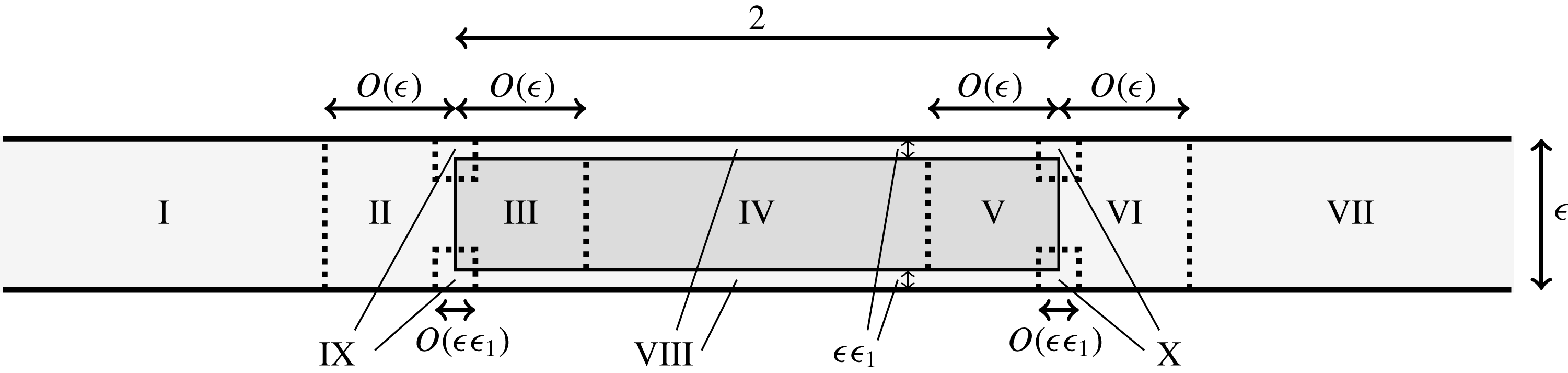
The extended boundary layer structure within the initial boundary layers for the flow problem when
 $1\ll Re\ll \unicode[STIX]{x1D716}^{-1}$
for (a) inflow and (b) outflow. The flow is from left to right. The relative size of each boundary layer has been exaggerated for illustrative purposes.
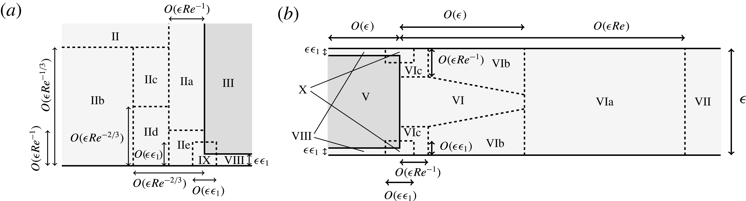
A.1 Thin gaps between the flat sides of the construct and the bioreactor
The thin gaps between the flat sides of the tissue construct and the bioreactor allow free movement of the tissue construct. However, the thin nature of the gaps results in a significant contribution towards the stress and torque acting on the construct from
 $\boldsymbol{f}_{f}$
and
 $\unicode[STIX]{x1D749}_{f}$
, respectively, defined in (2.16).
We consider the flow in the thin gap near
 $z=0$
, and note that there is an equivalent asymptotic region near
 $z=1$
. Our main goal is to determine the shear stress acting on the flat sides of the tissue construct, and our secondary goal is to show that the fluid flux from this region is of
 $O(\unicode[STIX]{x1D716}\unicode[STIX]{x1D716}_{1})$
, and thus unimportant to the remaining boundary layer analysis.
In region
 $\text{VIII}$
, we scale
 $z=\unicode[STIX]{x1D716}_{1}\hat{z}$
and
 $w=\unicode[STIX]{x1D716}_{1}{\hat{w}}$
. Then, the governing equation (2.12) becomes
 $$\begin{eqnarray}\displaystyle & \displaystyle O(\unicode[STIX]{x1D716}Re)=-p_{X}+\unicode[STIX]{x1D716}_{1}^{-2}u_{\hat{z}\hat{z}}, & \displaystyle\end{eqnarray}$$
 $$\begin{eqnarray}\displaystyle & \displaystyle O(\unicode[STIX]{x1D716}Re)=-p_{Y}+\unicode[STIX]{x1D716}_{1}^{-2}v_{\hat{z}\hat{z}}, & \displaystyle\end{eqnarray}$$
 $$\begin{eqnarray}\displaystyle & \displaystyle 0=-\unicode[STIX]{x1D716}_{1}^{-1}p_{\hat{z}}+O(\unicode[STIX]{x1D716}^{2}\unicode[STIX]{x1D716}_{1}^{-1}), & \displaystyle\end{eqnarray}$$
 $$\begin{eqnarray}\displaystyle & \displaystyle 0=u_{X}+v_{Y}+{\hat{w}}_{\hat{z}}, & \displaystyle\end{eqnarray}$$
 $\hat{z}=0$
and (2.15) on
 $\hat{z}=1$
.
Combining the scaling
 $w=\unicode[STIX]{x1D716}_{1}{\hat{w}}$
with (2.15a
) yields (A 24), the effective no-flux conditions on the flat sides of the construct. Additionally, the solution of
 $u$
and
 $v$
up to
 $O(\unicode[STIX]{x1D716}_{1}^{2})$
in terms of the pressure and the construct velocity is
 $$\begin{eqnarray}u\boldsymbol{e}_{X}+v\boldsymbol{e}_{Y}=\unicode[STIX]{x1D716}_{1}^{2}{\displaystyle \frac{\hat{z}(\hat{z}-1)}{2}}\unicode[STIX]{x1D735}_{\bot }p+(1-\hat{z})(1-\dot{\unicode[STIX]{x1D711}})\boldsymbol{e}_{z}\times \boldsymbol{X}+\hat{z}(\dot{R}\boldsymbol{e}_{X}+(\unicode[STIX]{x1D714}-\dot{\unicode[STIX]{x1D711}})\boldsymbol{e}_{z}\times \boldsymbol{r}),\end{eqnarray}$$
which allows us to determine
 $\unicode[STIX]{x1D748}\boldsymbol{\cdot }\boldsymbol{n}$
on the flat sides of the construct,
 $T_{2}$
and
 $T_{3}$
(defined in (2.17)). We note that the stress in the normal directions will cancel when summing the contributions on the top and bottom of the construct, but the shear contributions in the tangential directions will double. Thus, the effective stress on the flat sides of the construct is
 $$\begin{eqnarray}\unicode[STIX]{x1D748}\boldsymbol{\cdot }\boldsymbol{n}={\displaystyle \frac{2\unicode[STIX]{x1D716}}{\unicode[STIX]{x1D716}_{1}}}(-\dot{R}\boldsymbol{e}_{X}+R(1-\dot{\unicode[STIX]{x1D711}})\boldsymbol{e}_{Y}+(1-\unicode[STIX]{x1D714})\boldsymbol{e}_{z}\times \boldsymbol{r})+O(\unicode[STIX]{x1D716}_{1}\unicode[STIX]{x1D716}).\end{eqnarray}$$
As we do not require knowledge of
 $p$
to determine (A 3), it is not necessary to solve for the pressure within region
 $\text{VIII}$
. Hence, it is not necessary to solve for the flow variables in regions
 $\text{IX}$
and
 $\text{X}$
, which denote the transition regions into
 $\text{VIII}$
for inflow and outflow, respectively. For completeness, however, we note that the relevant scalings for regions
 $\text{IX}$
and
 $\text{X}$
are given by
 $z\sim \unicode[STIX]{x1D716}_{1}$
(or
 $1-z\sim \unicode[STIX]{x1D716}_{1}$
),
 $\sqrt{(X-R)^{2}+Y^{2}}-b\sim \unicode[STIX]{x1D716}\unicode[STIX]{x1D716}_{1}$
, and
 $w\sim \unicode[STIX]{x1D716}^{-1}$
. Integrating (A 2) over the gap thickness to obtain the asymptotic strength of the flux within the thin gaps, we note that the strength is of
 $O(\unicode[STIX]{x1D716}\unicode[STIX]{x1D716}_{1})$
. As we do not require flow results up to this order, we do not need further results from these regions.
A.2 Asymptotic regions near the curved boundary of the tissue construct
We now consider the flow problem near the curved interface of the construct. This involves the inner regions
 $\text{II}$
and
 $\text{III}$
for inflow, and the inner regions
 $\text{V}$
and
 $\text{VI}$
for outflow, as shown in figure 13. The further boundary layers within these initial inner regions when
 $1\ll Re\ll \unicode[STIX]{x1D716}^{-1}$
are shown in figure 14. As mentioned above, the version of this problem with stationary walls and no thin gap is investigated in detail in Dalwadi et al. (Reference Dalwadi, Chapman, Waters and Oliver2016). Thus, in this subsection we only present the salient differences that arise from introducing moving walls. We are interested in how the pressure and flow averaged over the bioreactor thickness vary across the boundary regions. This will allow us to determine the correct coupling conditions to apply in the reduced problem (the ‘outer regions’ in this boundary layer analysis) we consider in the main text.
It will be convenient to work in a third frame, where the tissue construct is stationary, and we refer to this as the frame relative to the construct motion. In moving to this frame from the laboratory frame, we translate the origin to the tissue construct centre, and rotate with angular velocity
 $\unicode[STIX]{x1D714}\boldsymbol{e}_{z}$
. Additionally, we introduce the curvilinear coordinates
 $(n,s,z)$
, such that
 $n=0$
on the curved interface of the construct,
 $T_{1}$
(defined in (2.17)). Increasing
 $n$
moves into the bulk fluid, and
 $s$
is the arclength around the boundary in the anticlockwise azimuthal direction. In the frame relative to the construct motion, we define the bulk and porous flow velocities as
 $\boldsymbol{u}^{rel}=u^{rel}\boldsymbol{n}+v^{rel}\boldsymbol{s}+w^{rel}\boldsymbol{e}_{z}$
and
 $\boldsymbol{Q}^{rel}=U^{rel}\boldsymbol{n}+V^{rel}\boldsymbol{s}+W^{rel}\boldsymbol{e}_{z}$
, respectively. Here,
 $\boldsymbol{n}=\boldsymbol{e}_{n}$
and
 $\boldsymbol{s}=\boldsymbol{e}_{s}$
are the unit vectors in the normal and azimuthal directions, respectively, and the velocity in the
 $z$
-direction has been scaled with
 $\unicode[STIX]{x1D716}$
, in the same manner as (2.11). The relationship between the velocities in the relative construct and laboratory frames is
 $$\begin{eqnarray}\boldsymbol{u}^{rel}=\boldsymbol{u}_{LF}-\boldsymbol{V}_{TC},\quad \boldsymbol{Q}^{rel}=\boldsymbol{Q}_{LF}-\boldsymbol{V}_{TC}.\end{eqnarray}$$
We then expand the fluid velocities and pressures as in (3.1). Thus, we have defined the outer problem in the frame relative to the construct motion.
The analysis to derive the leading-order coupling conditions in Dalwadi et al. (Reference Dalwadi, Chapman, Waters and Oliver2016) for stationary walls can be directly extended to moving walls. That is, we can deduce that the leading-order pressures and normal velocities averaged over the bioreactor thickness are continuous for the problem we consider here. This results in the coupling conditions
 $$\begin{eqnarray}p_{0}=P_{0},\quad \int _{0}^{1}\boldsymbol{u}_{0}^{rel}\boldsymbol{\cdot }\boldsymbol{n}\,\text{d}z=\int _{0}^{1}\boldsymbol{Q}_{0}^{rel}\boldsymbol{\cdot }\boldsymbol{n}\,\text{d}z.\end{eqnarray}$$
If we have an impermeable wall instead of a porous construct, as for the curved bioreactor edge, we can simply impose
 $\boldsymbol{Q}_{0}^{rel}\boldsymbol{\cdot }\boldsymbol{n}=0$
, to obtain
 $$\begin{eqnarray}\int _{0}^{1}\boldsymbol{u}_{0}^{rel}\boldsymbol{\cdot }\boldsymbol{n}\,\text{d}z=0.\end{eqnarray}$$
Moreover, at
 $O(\unicode[STIX]{x1D716}Re)$
the inflow problem from Dalwadi et al. (Reference Dalwadi, Chapman, Waters and Oliver2016) can also be directly extended to moving walls. This yields
 $$\begin{eqnarray}p_{1}=P_{1}\quad \text{on }T_{1}\text{ for }u_{0}^{rel}<0,\end{eqnarray}$$
for the pressure condition. Additionally, the normal flow in the outer regions at
 $O(\unicode[STIX]{x1D716}Re)$
is unchanged due to the variation in the leading-order azimuthal flow in the inflow inner regions over a length scale of
 $O(\unicode[STIX]{x1D716}/Re)$
. Thus, we also have
 $$\begin{eqnarray}\int _{0}^{1}\boldsymbol{u}_{1}^{rel}\boldsymbol{\cdot }\boldsymbol{n}\,\text{d}z=\int _{0}^{1}\boldsymbol{Q}_{1}^{rel}\boldsymbol{\cdot }\boldsymbol{n}\,\text{d}z\quad \text{on }T_{1}\text{ for }u_{0}^{rel}<0.\end{eqnarray}$$
The results from Dalwadi et al. (Reference Dalwadi, Chapman, Waters and Oliver2016) can also be easily extended to determine that the shear stress in the azimuthal direction acting on the interface for inflow is
 $$\begin{eqnarray}\boldsymbol{s}\boldsymbol{\cdot }(\unicode[STIX]{x1D748}\boldsymbol{\cdot }\boldsymbol{n})\sim -(\unicode[STIX]{x1D716}Re)v_{0}^{rel}u_{0}^{rel}\quad \text{on }T_{1}\text{ for }u_{0}^{rel}<0.\end{eqnarray}$$
However, a little extra work is required to extend the outflow coupling conditions for the
 $O(\unicode[STIX]{x1D716}Re)$
correction terms in Dalwadi et al. (Reference Dalwadi, Chapman, Waters and Oliver2016) from stationary walls to moving walls. The outflow boundary layer structure from Dalwadi et al. (Reference Dalwadi, Chapman, Waters and Oliver2016) is the same, and it remains to solve a slightly extended problem.
A.2.1 Outflow
For outflow, plug flow in the porous medium transitions to Poiseuille/Couette flow in the bulk flow due to the wall motion, and this transition occurs in region
 $\text{VIa}$
(see figure 14) at leading order. As the pressure and flow changes over an
 $O(\unicode[STIX]{x1D716}Re)$
length scale, a leading-order flow and pressure variation in this region can cause an
 $O(\unicode[STIX]{x1D716}Re)$
variation in the coupling conditions between the outer regions, as we will show. This is in contrast to the inflow problem where the change occurs over a smaller length scale, resulting in continuous coupling conditions for the pressure and flux averaged over the bioreactor thickness. We note that this longer length scale for outflow also means that the stress acting on the interface for outflow is asymptotically smaller than for inflow.
We note that, in the frame relative to the construct motion, the no-slip condition on
 $z=0,1$
becomes
 $$\begin{eqnarray}\boldsymbol{u}^{rel}=\boldsymbol{u}^{slip}:=\boldsymbol{e}_{z}\times \boldsymbol{X}-\boldsymbol{V}_{TC}=(1-\unicode[STIX]{x1D714})\boldsymbol{e}_{z}\times \boldsymbol{r}-\dot{R}\boldsymbol{e}_{X}+R(1-\dot{\unicode[STIX]{x1D711}})\boldsymbol{e}_{Y}.\end{eqnarray}$$
Additionally, at the construct interface, we have plug flow (details of this can be found in Dalwadi et al. (Reference Dalwadi, Chapman, Waters and Oliver2016)). Thus, the conditions at the interface are
 $$\begin{eqnarray}u_{0}^{rel}=-KP_{0n}(0,s,t),\quad v_{0}^{rel}=0,\quad w_{0}^{rel}=0,\quad p_{1}=P_{1}(0,s,t)\quad \text{on }n=0,\end{eqnarray}$$
noting that
 $P_{0n}<0$
and thus
 $u_{0}^{rel}>0$
for outflow.
In region
 $\text{VIa}$
, we scale
 $$\begin{eqnarray}\left.\begin{array}{@{}c@{}}\displaystyle n=(-KP_{0n}(0,s,t)\unicode[STIX]{x1D716}Re)\widetilde{N},\quad u_{0}^{rel}=(-KP_{0n}(0,s,t))\widetilde{u},\quad w_{0}^{rel}=(1/(\unicode[STIX]{x1D716}Re))\widetilde{w},\\ \displaystyle v_{0}^{rel}=p_{0s}(0,s,t)\left(\widetilde{v}^{(a)}-{\displaystyle \frac{z(1-z)}{2}}\right)+\boldsymbol{s}\boldsymbol{\cdot }\boldsymbol{u}^{slip}(\widetilde{v}^{(b)}+1),\\ \displaystyle p_{1}=P_{1}(0,s,t)+(-KP_{0n}(0,s,t))^{2}\widetilde{p},\end{array}\right\}\end{eqnarray}$$
to obtain the leading-order boundary layer equations
 $$\begin{eqnarray}\widetilde{u}\widetilde{u}_{\widetilde{N}}+\widetilde{w}\widetilde{u}_{z}=-\widetilde{p}_{\widetilde{N}}+\widetilde{u}_{zz},\quad \widetilde{u}\widetilde{v}_{\widetilde{N}}^{(i)}+\widetilde{w}\widetilde{v}_{z}^{(i)}=\widetilde{v}_{zz}^{(i)},\quad 0=-\widetilde{p}_{z},\quad \widetilde{u}_{\widetilde{N}}+\widetilde{w}_{z}=0,\end{eqnarray}$$
for
 $(N,z)\in \mathbb{R}^{+}\times (0,1)$
, and
 $i\in \{a,b\}$
. We note that the second equation in (A 11a
) decouples from the remaining three equations. On the cell walls, the no-slip conditions (A 9a
) become
 $$\begin{eqnarray}\widetilde{u}={\mathcal{A}},\quad \widetilde{v}^{(a)}=0,\quad \widetilde{v}^{(b)}=0,\quad \widetilde{w}=0,\end{eqnarray}$$
for
 $\widetilde{N}>0$
and
 $z=0,1$
, Near the construct interface, we use the matching conditions
 $$\begin{eqnarray}\left.\begin{array}{@{}c@{}}\displaystyle \widetilde{u}\sim 1+2\tilde{\unicode[STIX]{x1D6FD}}({\mathcal{A}})\widetilde{N}^{1/2},\quad \widetilde{v}^{(a)}\sim {\displaystyle \frac{z(1-z)}{2}},\quad \widetilde{v}^{(b)}\sim -1,\\ \displaystyle \widetilde{w}\sim {\displaystyle \frac{\tilde{\unicode[STIX]{x1D6FD}}({\mathcal{A}})(1-2z)}{2\widetilde{N}^{1/2}}},\quad \widetilde{p}\sim -2\tilde{\unicode[STIX]{x1D6FD}}({\mathcal{A}})\widetilde{N}^{1/2}\quad \text{as }\widetilde{N}\rightarrow 0^{+}\quad \text{for }z\in (0,1).\end{array}\right\}\end{eqnarray}$$
Here, we define
 $$\begin{eqnarray}{\mathcal{A}}(s,t):={\displaystyle \frac{\boldsymbol{n}\boldsymbol{\cdot }\boldsymbol{u}^{slip}(0,s,t)}{(-KP_{0n}(0,s,t))}},\end{eqnarray}$$
and
 $\tilde{\unicode[STIX]{x1D6FD}}({\mathcal{A}})$
arises from the leading-order problem in region
 $\text{VIb}$
. The details of the flow problem in region
 $\text{VIb}$
, essentially the classic Prandtl boundary layer problem (Prandtl Reference Prandtl and Krazer1904) reduced to the Blasius equation (Blasius Reference Blasius1908), and how it relates to the remaining regions are given in Dalwadi et al. (Reference Dalwadi, Chapman, Waters and Oliver2016) for stationary walls. Determining
 $\tilde{\unicode[STIX]{x1D6FD}}$
in our problem requires extending this analysis to moving walls. To obtain
 $\tilde{\unicode[STIX]{x1D6FD}}({\mathcal{A}})$
, we must solve the problem
 $$\begin{eqnarray}2g^{\prime \prime \prime }(\unicode[STIX]{x1D702})+g^{\prime \prime }(\unicode[STIX]{x1D702})g(\unicode[STIX]{x1D702})=0,\quad g(0)=0,\quad g^{\prime }(0)={\mathcal{A}},\quad g^{\prime }(\infty )=1:\end{eqnarray}$$
then
 $\tilde{\unicode[STIX]{x1D6FD}}({\mathcal{A}})$
is defined as
 $$\begin{eqnarray}\tilde{\unicode[STIX]{x1D6FD}}({\mathcal{A}})=\lim _{\unicode[STIX]{x1D702}\rightarrow \infty }(\unicode[STIX]{x1D702}-g(\unicode[STIX]{x1D702})).\end{eqnarray}$$
We note that existence and uniqueness of the solution to (A 13) for
 ${\mathcal{A}}\geqslant 0$
is shown in Callegari & Friedman (Reference Callegari and Friedman1968) and Callegari & Nachman (Reference Callegari and Nachman1978), and existence with two solutions for
 ${\mathcal{A}}\in (-{\mathcal{A}}^{\ast },0)$
, and no values of
 $\tilde{\unicode[STIX]{x1D6FD}}$
for
 ${\mathcal{A}}<-{\mathcal{A}}^{\ast }$
, where
 ${\mathcal{A}}^{\ast }\approx 0.3541$
, is shown in Hussaini & Lakin (Reference Hussaini and Lakin1986) and Hussaini, Lakin & Nachman (Reference Hussaini, Lakin and Nachman1987). Thus, this problem only has a solution for
 ${\mathcal{A}}\geqslant -{\mathcal{A}}^{\ast }$
.
The function
 $\tilde{\unicode[STIX]{x1D6FD}}({\mathcal{A}})$
, defined in (A 15). For
 ${\mathcal{A}}<0$
, we find that
 $\tilde{\unicode[STIX]{x1D6FD}}({\mathcal{A}})$
is not unique. We denote the stable (lower) solution with a solid line and the unstable (upper) solution with a dashed line, and mark the point where these solution curves meet with an asterisk. Moreover, we note that there is no solution for
 ${\mathcal{A}}<-{\mathcal{A}}^{\ast }$
, where
 ${\mathcal{A}}^{\ast }\approx 0.3541$
.
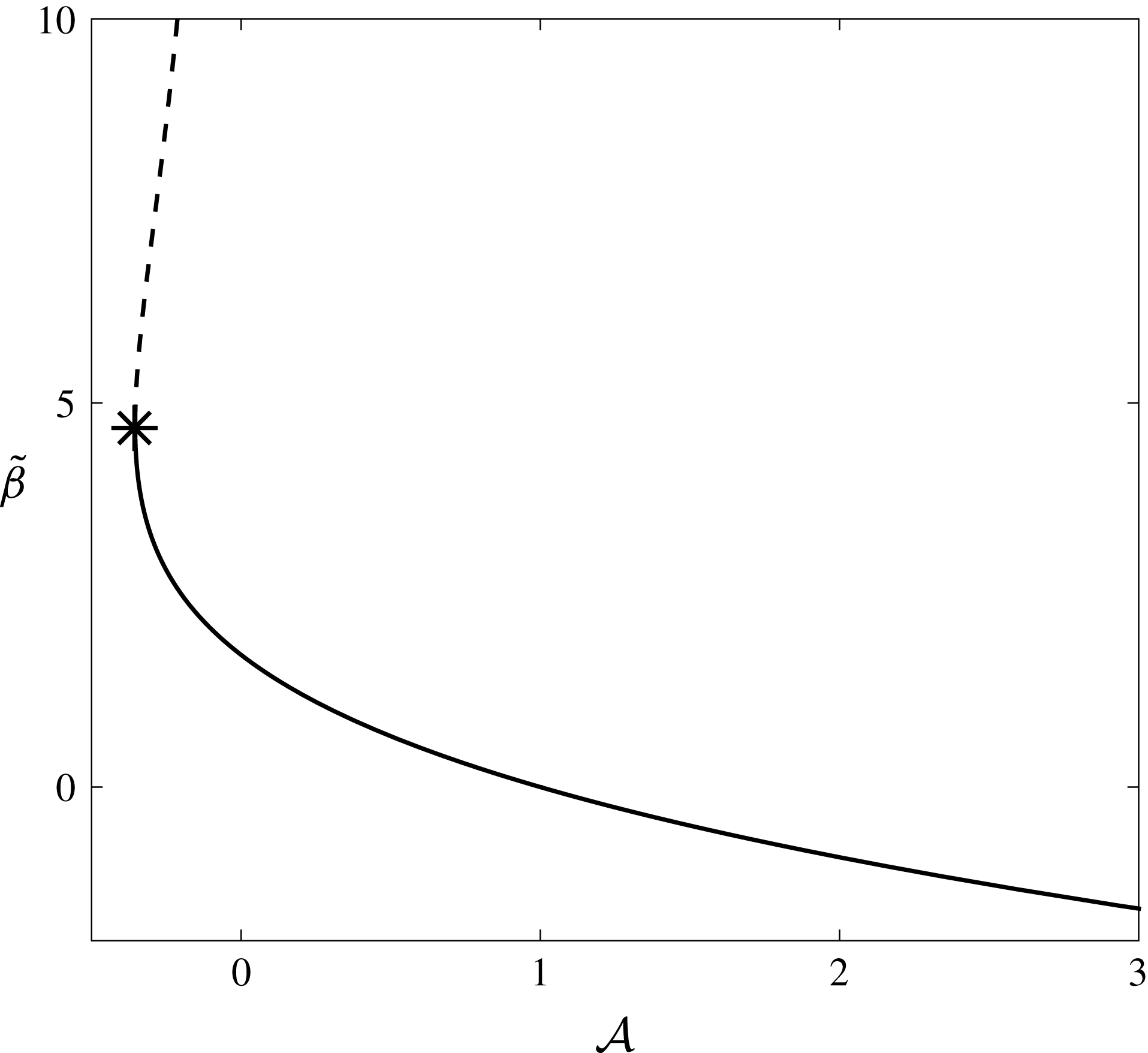
To efficiently determine
 ${\mathcal{A}}$
, we modify the trick used by Töpfer (Reference Töpfer1912) and turn the boundary value problem (A 13) into an initial value problem by exploiting the invariance in the system. That is, we solve the initial value problem
 $$\begin{eqnarray}2\bar{g}^{\prime \prime \prime }(\unicode[STIX]{x1D702})+\bar{g}^{\prime \prime }(\unicode[STIX]{x1D702})\bar{g}(\unicode[STIX]{x1D702})=0,\quad \bar{g}(0)=0,\quad \bar{g}^{\prime }(0)=\unicode[STIX]{x1D6FE},\quad \bar{g}^{\prime \prime }(0)=\operatorname{sign}(1-{\mathcal{A}}),\end{eqnarray}$$
for
 $\unicode[STIX]{x1D702}>0$
, using a range of values of
 $\unicode[STIX]{x1D6FE}$
, and note that the far-field behaviour of this function is
 $$\begin{eqnarray}\bar{g}\sim {\displaystyle \frac{\unicode[STIX]{x1D6FE}}{{\mathcal{A}}}}\unicode[STIX]{x1D702}-\tilde{\unicode[STIX]{x1D6FD}}({\mathcal{A}})\sqrt{{\displaystyle \frac{{\mathcal{A}}}{\unicode[STIX]{x1D6FE}}}}+\text{exponentially small terms}\quad \text{as }\unicode[STIX]{x1D702}\rightarrow \infty .\end{eqnarray}$$
We solve (A 15a
) numerically, encountering the same number of solutions for a given
 ${\mathcal{A}}$
as predicted in Callegari & Friedman (Reference Callegari and Friedman1968), Callegari & Nachman (Reference Callegari and Nachman1978), Hussaini & Lakin (Reference Hussaini and Lakin1986), Hussaini et al. (Reference Hussaini, Lakin and Nachman1987) (see figure 15). We will use values of
 $\tilde{\unicode[STIX]{x1D6FD}}$
from the solid curve in figure 15, taking the lower branch of the non-unique solutions (corresponding to larger values of the skin friction) as this branch continuously varies from the unique solutions for
 ${\mathcal{A}}\geqslant 0$
. We note that as the movement of the tissue construct is governed by the forces acting upon it, the normal wall slip velocity does not tend to oppose the normal velocity leaving the construct for our problem. Hence, we do not encounter extreme values of
 ${\mathcal{A}}$
in our problem;
 ${\mathcal{A}}$
tends to stay within
 $(0,3)$
, though very occasionally strays beyond these limits. When it does, we extrapolate the corresponding coupling conditions using a cubic spline. We also note that very small values of
 $K$
(corresponding to a near impermeable construct) would result in large values of
 ${\mathcal{A}}$
. However, in that limit, the assumption that there is an
 $O(1)$
flow though the construct would break down, and we would be in the small local Reynolds number limit. This limit was also considered in Dalwadi et al. (Reference Dalwadi, Chapman, Waters and Oliver2016) for stationary walls.
Finally, we note that the far-field conditions of (A 11a,b
) match with region
 $\text{VII}$
, the outer outflow region, and are
 $$\begin{eqnarray}\left.\begin{array}{@{}c@{}}\displaystyle \widetilde{u}\rightarrow {\mathcal{A}}+{\displaystyle \frac{z(z-1)p_{0n}(0,s,t)}{2(-KP_{0n}(0,s,t))}},\quad \widetilde{v}^{(a)}\rightarrow 0,\quad \widetilde{v}^{(b)}\rightarrow 0,\quad \widetilde{w}\rightarrow 0,\\ \displaystyle \widetilde{p}\sim {\displaystyle \frac{p_{0n}(0,s,t)\widetilde{N}}{(-KP_{0n}(0,s,t))}}+\unicode[STIX]{x1D6F1}({\mathcal{A}};s,t)\quad \text{as }\widetilde{N}\rightarrow \infty .\end{array}\right\}\end{eqnarray}$$
Here,
 $\unicode[STIX]{x1D6F1}$
is the function required to couple the first-correction pressures in the outer regions. That is, rearranging (A 10) and using the far-field results (A 16a
) leads to the outer coupling condition for outflow at this order:
 $$\begin{eqnarray}p_{1}-P_{1}=(-KP_{0n}(0,s,t))^{2}\unicode[STIX]{x1D6F1}({\mathcal{A}};s,t)\quad \text{for }u_{0}^{rel}>0.\end{eqnarray}$$
We discuss our numerical solution for
 $\unicode[STIX]{x1D6F1}$
below.
To determine the coupling condition for the normal velocity averaged over the
 $z$
-direction, we note that an
 $O(\unicode[STIX]{x1D716}Re)$
difference in normal velocity can be obtained by a leading-order variation in the azimuthal velocity over a length scale of
 $O(\unicode[STIX]{x1D716}Re)$
. This can be formally deduced by integrating the continuity equations (2.12d
) and (2.13d
) over the inner regions, as shown in Dalwadi et al. (Reference Dalwadi, Chapman, Waters and Oliver2016). Using the scalings (A 10), the equivalent relationship here is
 $$\begin{eqnarray}\int _{0}^{1}(\boldsymbol{u}_{1}^{rel}-\boldsymbol{Q}_{1}^{rel})\boldsymbol{\cdot }\boldsymbol{n}\,\text{d}z={\displaystyle \frac{\unicode[STIX]{x2202}}{\unicode[STIX]{x2202}s}}(KP_{0n}(0,s,t)\{p_{0s}(0,s,t)\unicode[STIX]{x1D6EC}_{a}+\boldsymbol{s}\boldsymbol{\cdot }\boldsymbol{u}^{slip}\unicode[STIX]{x1D6EC}_{b}\})\quad \text{for }u_{0}^{rel}>0,\end{eqnarray}$$
where
 $$\begin{eqnarray}\displaystyle & \displaystyle \unicode[STIX]{x1D6EC}_{a}({\mathcal{A}};s,t)=\int _{0}^{\infty }\int _{0}^{1}\widetilde{v}^{(a)}\,\text{d}z\,\text{d}\widetilde{N}, & \displaystyle\end{eqnarray}$$
 $$\begin{eqnarray}\displaystyle & \displaystyle \unicode[STIX]{x1D6EC}_{b}({\mathcal{A}};s,t)=\int _{0}^{\infty }\int _{0}^{1}\widetilde{v}^{(b)}\,\text{d}z\,\text{d}\widetilde{N}, & \displaystyle\end{eqnarray}$$
where
 $\widetilde{v}^{(a)}$
and
 $\widetilde{v}^{(b)}$
are solved by (A 11). We follow Dalwadi et al. (Reference Dalwadi, Chapman, Waters and Oliver2016) and solve for
 $\widetilde{u}$
,
 $\widetilde{w}$
, and
 $\widetilde{p}$
using the second-order central finite-difference scheme described in Bodoia & Osterle (Reference Bodoia and Osterle1961), implemented for moving walls, enabling us to determine
 $\unicode[STIX]{x1D6F1}$
. Then, we use these results to solve for
 $\widetilde{v}^{(a)}$
and
 $\widetilde{v}^{(b)}$
using a second-order central finite-difference scheme, allowing us to obtain
 $\unicode[STIX]{x1D6EC}_{a}$
and
 $\unicode[STIX]{x1D6EC}_{b}$
via quadrature. We show our results for these three functions in figure 16. As we discussed above,
 ${\mathcal{A}}$
tends to stay within
 $(0,3)$
and we extrapolate the corresponding coupling conditions using a cubic spline on the rare occasions that
 ${\mathcal{A}}$
strays out of this range (dashed lines on figure 16).
The three functions
 $\unicode[STIX]{x1D6F1}$
,
 $\unicode[STIX]{x1D6EC}_{a}$
, and
 $\unicode[STIX]{x1D6EC}_{b}$
, defined in (A 16a
), (A 17b
), and (A 17c
), respectively. These functions are used to evaluate the coupling conditions (defined in (A 16b
) and (A 17a
)) between the moving outer regions of the tissue construct and the bulk bioreactor flow. The coupling conditions have been reduced to functions of a single parameter,
 ${\mathcal{A}}$
, defined in (A 12). The solid lines are calculated from the definitions (A 16a
), (A 17b
), and (A 17c
), and the dashed lines represent the extrapolation we discuss in the main text.
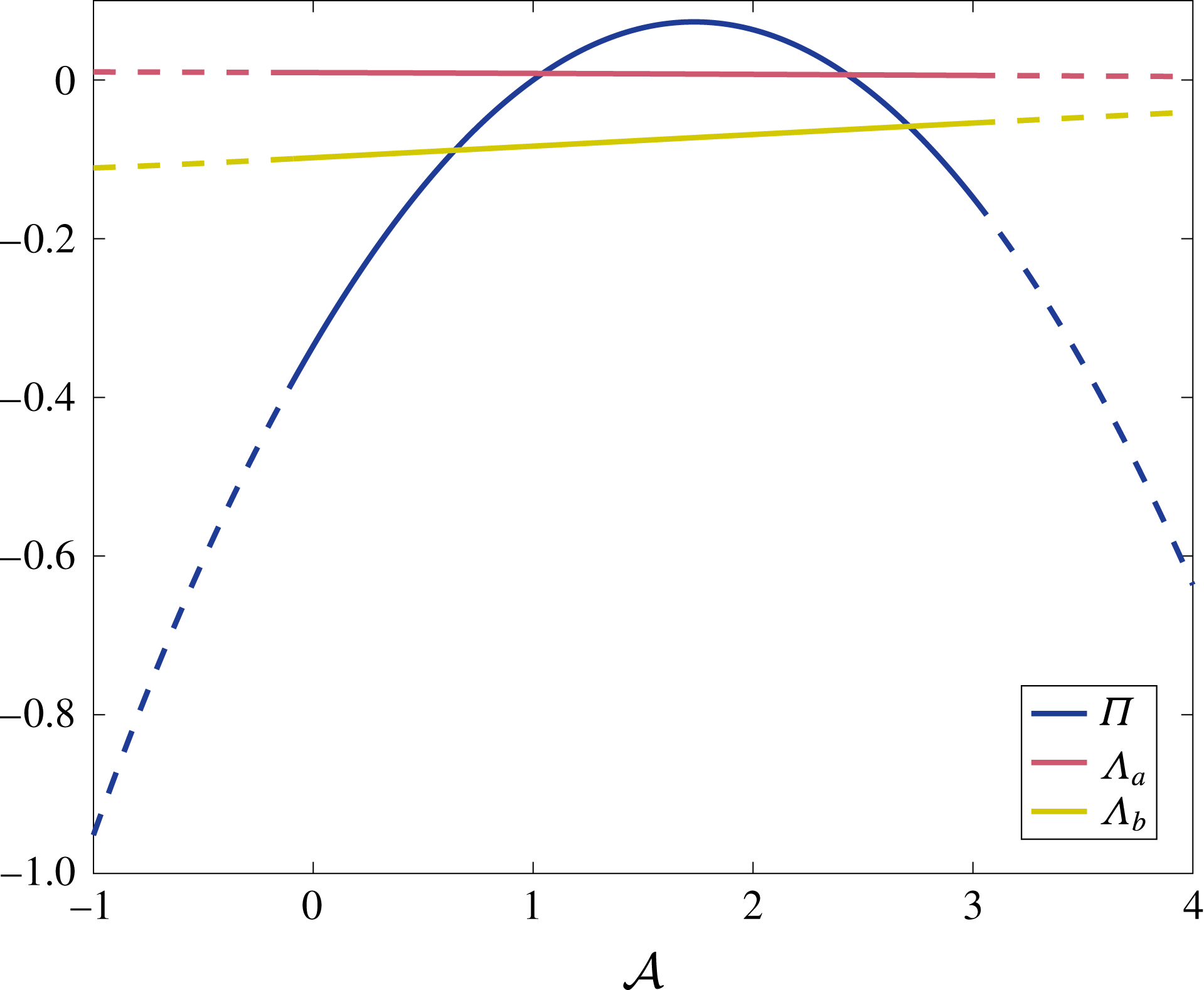
For an impermeable wall instead of a porous construct, the condition is the same as for leading order. That is, we use
 $\boldsymbol{Q}^{rel}\boldsymbol{\cdot }\boldsymbol{n}=0$
in (A 7b
) and (A 17a
) (along with
 $K=0$
for the latter), to obtain
 $$\begin{eqnarray}\int _{0}^{1}\boldsymbol{u}_{1}^{rel}\boldsymbol{\cdot }\boldsymbol{n}\,\text{d}z=0.\end{eqnarray}$$
Thus, we have determined the coupling conditions for the flow problem up to
 $O(\unicode[STIX]{x1D716}Re)$
. The leading-order coupling conditions are given by (A 5). The first-correction coupling conditions are given by (A 7) for inflow, and by (A 16b
)–(A 17). Our asymptotic analysis and scaling choices have reduced the problem of determining the coupling conditions significantly. That is, we are able to obtain the details we require by numerically solving a system for one dimensionless parameter, namely
 ${\mathcal{A}}$
.
A.3 Deriving the flow problem
We now derive the reduced flow problem we present and solve in § 3. We start by substituting the asymptotic expansions (3.1) into the bulk flow equations (2.12) and the interior flow equations (2.13). At
 $O(1)$
, in the bulk flow region we have
 $$\begin{eqnarray}p_{0X}=u_{0zz},\quad p_{0Y}=v_{0zz},\quad 0=-p_{0z},\quad \unicode[STIX]{x1D735}\boldsymbol{\cdot }\boldsymbol{u}_{0}=0,\end{eqnarray}$$
in the interior flow region we have
 $$\begin{eqnarray}\displaystyle & \displaystyle U_{0}-\dot{R}-(\dot{\unicode[STIX]{x1D711}}-\unicode[STIX]{x1D714})Y=-KP_{0X}, & \displaystyle\end{eqnarray}$$
 $$\begin{eqnarray}\displaystyle & \displaystyle V_{0}+(\dot{\unicode[STIX]{x1D711}}-\unicode[STIX]{x1D714})(X-R)=-KP_{0Y}, & \displaystyle\end{eqnarray}$$
 $$\begin{eqnarray}\displaystyle & \displaystyle 0=-KP_{0z}, & \displaystyle\end{eqnarray}$$
 $$\begin{eqnarray}\displaystyle & \displaystyle \unicode[STIX]{x1D735}\boldsymbol{\cdot }\boldsymbol{Q}_{0}=0. & \displaystyle\end{eqnarray}$$
At
 $O(\unicode[STIX]{x1D716}Re)$
, in the bulk flow region we have
 $$\begin{eqnarray}\displaystyle & \displaystyle \dot{u}_{0}+(\boldsymbol{u}_{0}\boldsymbol{\cdot }\unicode[STIX]{x1D735})u_{0}-2\dot{\unicode[STIX]{x1D711}}v_{0}-\ddot{\unicode[STIX]{x1D711}}Y-\dot{\unicode[STIX]{x1D711}}^{2}X=-p_{1X}+u_{1zz}, & \displaystyle\end{eqnarray}$$
 $$\begin{eqnarray}\displaystyle & \displaystyle \dot{v}_{0}+(\boldsymbol{u}_{0}\boldsymbol{\cdot }\unicode[STIX]{x1D735})v_{0}+2\dot{\unicode[STIX]{x1D711}}u_{0}+\ddot{\unicode[STIX]{x1D711}}X-\dot{\unicode[STIX]{x1D711}}^{2}Y=-p_{1Y}+v_{1zz}, & \displaystyle\end{eqnarray}$$
 $$\begin{eqnarray}\displaystyle & \displaystyle 0=-p_{1z}, & \displaystyle\end{eqnarray}$$
 $$\begin{eqnarray}\displaystyle & \displaystyle \unicode[STIX]{x1D735}\boldsymbol{\cdot }\boldsymbol{u}_{1}=0, & \displaystyle\end{eqnarray}$$
 $$\begin{eqnarray}U_{1}=-KP_{1X},\quad V_{1}=-KP_{1Y},\quad 0=-KP_{1z},\quad \unicode[STIX]{x1D735}\boldsymbol{\cdot }\boldsymbol{Q}_{1}=0.\end{eqnarray}$$
As is standard with the lubrication equations, we are able to impose the no-slip boundary conditions (2.14) on the flat surfaces of the bioreactor, as follows
 $$\begin{eqnarray}\boldsymbol{u}_{0}=(1-\dot{\unicode[STIX]{x1D711}})\boldsymbol{e}_{z}\times \boldsymbol{X},\quad \boldsymbol{u}_{1}=\mathbf{0}\quad \text{on }\overline{S}.\end{eqnarray}$$
On
 $\overline{T}$
, the flat surfaces of the tissue construct, we see from § A.1 that the continuity of flux condition (2.15a
) reduces to no flux through the boundary
 $$\begin{eqnarray}W_{0}=0,\quad W_{1}=0\quad \text{on }\overline{T},\end{eqnarray}$$
and the remaining conditions on this boundary are not required. We derive the effective conditions to be applied at the curved construct interface in § A.2. At leading order, the effective coupling conditions are (A 5). At
 $O(\unicode[STIX]{x1D716}Re)$
, the effective coupling conditions are (A 7) for the averaged flow moving into the construct relative to its motion, and (A 16b
) and (A 17) for the averaged flow moving out of the construct relative to its motion. At the curved bioreactor edge, the effective boundary conditions are (A 6) for leading order and (A 18) for first correction.
A.3.1 Deriving the
$O(1)$
flow equations

Solving (A 19a–c
) subject to (A 23a
) in the
 $X$
- and
 $Y$
-directions, we obtain
 $$\begin{eqnarray}(u_{0},v_{0})=(1-\dot{\unicode[STIX]{x1D711}})\boldsymbol{e}_{z}\times \boldsymbol{X}+f_{1}(z)(p_{0X},p_{0Y}),\quad f_{1}(z)={\displaystyle \frac{z(z-1)}{2}}.\end{eqnarray}$$
Substituting (A 25) into (A 19d
), integrating with respect to
 $z$
, and using (A 23a
) in the
 $z$
-direction, we obtain
 $$\begin{eqnarray}w_{0}\equiv 0,\quad 0=\unicode[STIX]{x1D6FB}_{\bot }^{2}p_{0},\end{eqnarray}$$
where we reiterate that
 $\unicode[STIX]{x1D6FB}_{\bot }^{2}=\unicode[STIX]{x2202}_{XX}+\unicode[STIX]{x2202}_{YY}$
.
The Darcy velocity in terms of the fluid pressure inside the construct is already given by (A 20a,b
). Hence, our tasks within the construct are to formulate a governing equation for
 $P_{0}$
and to determine
 $W_{0}$
. Proceeding as for the bulk flow, we substitute (A 20a,b
) into (A 20d
), integrate with respect to
 $z$
, and use (A 24a
) to determine that
 $$\begin{eqnarray}W_{0}\equiv 0,\quad 0=\unicode[STIX]{x1D6FB}_{\bot }^{2}P_{0}.\end{eqnarray}$$
Thus, (A 25)–(A 27) gives the leading-order flow in terms of the fluid pressure, and the governing equations for the latter. In conjunction with (A 5), these yield the leading-order system we state and solve in § 3.
A.3.2 Deriving the
$O(\unicode[STIX]{x1D716}Re)$
flow equations

At
 $O(\unicode[STIX]{x1D716}Re)$
, the analysis of the Darcy flow equations (A 22) is the same as for leading order, and we deduce that
 $$\begin{eqnarray}W_{1}\equiv 0,\quad 0=\unicode[STIX]{x1D6FB}_{\bot }^{2}P_{1}.\end{eqnarray}$$
The bulk flow equations at this order are given by (A 21). By integrating twice with respect to
 $z$
, and using the no-slip boundary conditions (A 23b
) on
 $z=0$
,
 $1$
, the in-plane fluid velocity is given in terms of the fluid pressure as follows
 $$\begin{eqnarray}u_{1}\boldsymbol{e}_{X}+v_{1}\boldsymbol{e}_{Y}=f_{1}(z)\boldsymbol{A}(X,Y,t)+f_{2}(z)\boldsymbol{B}(X,Y,t)+f_{3}(z)\boldsymbol{C}(X,Y,t),\end{eqnarray}$$
where
 $$\begin{eqnarray}f_{2}(z)={\displaystyle \frac{f_{1}(z)(z^{2}-z-1)}{12}},\quad f_{3}(z)={\displaystyle \frac{f_{1}(z)(2z^{4}-4z^{3}+z^{2}+z+1)}{120}},\end{eqnarray}$$
and
 $$\begin{eqnarray}\displaystyle & \displaystyle \boldsymbol{A}(X,Y,t)=\unicode[STIX]{x1D735}(p_{1}-{\textstyle \frac{1}{2}}(X^{2}+Y^{2})), & \displaystyle\end{eqnarray}$$
 $$\begin{eqnarray}\displaystyle & \displaystyle \boldsymbol{B}(X,Y,t)=\unicode[STIX]{x1D735}(\dot{p}_{0}+(1-\dot{\unicode[STIX]{x1D711}})(\boldsymbol{e}_{z}\times \boldsymbol{X})\boldsymbol{\cdot }\unicode[STIX]{x1D735}p_{0})-2\unicode[STIX]{x1D735}\times (p_{0}\boldsymbol{e}_{z}), & \displaystyle\end{eqnarray}$$
 $$\begin{eqnarray}\displaystyle & \displaystyle \boldsymbol{C}(X,Y,t)=\unicode[STIX]{x1D735}\left({\textstyle \frac{1}{2}}|\unicode[STIX]{x1D735}p_{0}|^{2}\right), & \displaystyle\end{eqnarray}$$
 $f_{1}(z)$
is defined in (A 25). From the continuity equation (A 21d
), the solution for
 $w_{1}$
is given by
 $$\begin{eqnarray}w_{1}=-\unicode[STIX]{x1D6FB}_{\bot }^{2}\left(\left(p_{1}-{\displaystyle \frac{1}{2}}(X^{2}+Y^{2})\right)\int _{0}^{z}f_{1}(\unicode[STIX]{x1D709})\,\text{d}\unicode[STIX]{x1D709}+{\displaystyle \frac{1}{2}}|\unicode[STIX]{x1D735}p_{0}|^{2}\int _{0}^{z}f_{3}(\unicode[STIX]{x1D709})\,\text{d}\unicode[STIX]{x1D709}\right),\end{eqnarray}$$
where we use the fact that
 $\boldsymbol{B}$
is solenoidal. By setting
 $z=1$
in (A 32), we obtain the governing equation (3.15a
) for the first correction to the pressure. In the boundary regions, we note that the velocity components in the
 $\boldsymbol{e}_{z}$
direction only arise at the order where inertial terms are present. This is also true with stationary walls for both solid (Thompson Reference Thompson1968; Balsa Reference Balsa1998) and porous obstacles (Dalwadi et al.
Reference Dalwadi, Chapman, Waters and Oliver2016) in Hele-Shaw cells.
The average flux boundary conditions (3.7a ) and (3.16c ) are determined by integrating (A 29) over the bioreactor thickness to obtain
 $$\begin{eqnarray}\int _{0}^{1}\boldsymbol{u}_{1}\,\text{d}z=-{\displaystyle \frac{1}{12}}\unicode[STIX]{x1D735}\unicode[STIX]{x1D6F9}+{\displaystyle \frac{\boldsymbol{B}}{120}},\end{eqnarray}$$
which allows us to deduce (3.7a ) and (3.16c ), where we use (3.4a ) to simplify the first of these.
To calculate the second term in (A 31b ), we note that
 $$\begin{eqnarray}X\boldsymbol{e}_{X}+Y\boldsymbol{e}_{Y}={\displaystyle \frac{(\cosh (\unicode[STIX]{x1D6FC}-\unicode[STIX]{x1D6FC}_{1})\cos \unicode[STIX]{x1D6FD}-\cosh \unicode[STIX]{x1D6FC}_{1})\boldsymbol{e}_{\unicode[STIX]{x1D6FC}}+(\sinh (\unicode[STIX]{x1D6FC}-\unicode[STIX]{x1D6FC}_{1})\sin \unicode[STIX]{x1D6FD})\boldsymbol{e}_{\unicode[STIX]{x1D6FD}}}{\cosh \unicode[STIX]{x1D6FC}-\cos \unicode[STIX]{x1D6FD}}},\end{eqnarray}$$
obtained using (3.8) and moving from unit vectors in
 $(X,Y)$
to
 $(\unicode[STIX]{x1D6FC},\unicode[STIX]{x1D6FD})$
. Finally, we highlight that the bipolar transformation defined in (3.8) and (3.9) is time-dependent. Hence, when calculating
 $\dot{p}_{0}$
in (A 31b
), it is helpful to use the alternative bipolar definition
 $$\begin{eqnarray}\cosh \unicode[STIX]{x1D6FC}_{1}={\displaystyle \frac{1+R^{2}-b^{2}}{2R}},\quad \cosh \unicode[STIX]{x1D6FC}_{2}={\displaystyle \frac{1-R^{2}-b^{2}}{2Rb}},\end{eqnarray}$$
to obtain the following results
 $$\begin{eqnarray}{\displaystyle \frac{\text{d}\unicode[STIX]{x1D6FC}_{1}}{\text{d}t}}=-{\displaystyle \frac{\dot{R}\coth \unicode[STIX]{x1D6FC}_{2}}{R}},\quad {\displaystyle \frac{\text{d}\unicode[STIX]{x1D6FC}_{2}}{\text{d}t}}=-{\displaystyle \frac{\dot{R}\coth \unicode[STIX]{x1D6FC}_{1}}{R}}.\end{eqnarray}$$
Appendix B. Asymptotic behaviour of
$\unicode[STIX]{x1D6FE}_{1}(R)$

In the limit of small
 $R$
, we see from (A 35) that
 $\unicode[STIX]{x1D6FC}_{1}$
and
 $\unicode[STIX]{x1D6FC}_{2}$
are large. Thus, in this limit, (4.6b
) becomes
 $$\begin{eqnarray}\unicode[STIX]{x1D6FE}_{1}(R)={\displaystyle \frac{6}{\tanh (\unicode[STIX]{x1D6FC}_{2}-\unicode[STIX]{x1D6FC}_{1})+12K}}+O(\text{e}^{-2\unicode[STIX]{x1D6FC}_{2}}).\end{eqnarray}$$
Taking the logarithm of both sides of (3.9a ), we additionally deduce that
 $$\begin{eqnarray}\unicode[STIX]{x1D6FC}_{2}-\unicode[STIX]{x1D6FC}_{1}\sim -\log b\quad \text{as }R\rightarrow 0^{+}.\end{eqnarray}$$
Substituting (B 2) into (B 1), we obtain (4.7a ).
In the limit of
 $R\rightarrow (1-b)^{-}$
, corresponding to the construct edge getting close to the bioreactor edge, the analysis is a little more involved. In this limit,
 $\unicode[STIX]{x1D6FC}_{1}$
and
 $\unicode[STIX]{x1D6FC}_{2}$
are small, and thus the infinite sum (4.6b
) converges more slowly. More formally, setting
 $R=1-b-\unicode[STIX]{x1D6FF}^{2}b/(2(1-b))$
, where
 $\unicode[STIX]{x1D6FF}\ll 1$
is an artificially small parameter, we use (A 35) to deduce that
 $\unicode[STIX]{x1D6FC}_{1}\sim b\unicode[STIX]{x1D6FF}/(1-b)$
and
 $\unicode[STIX]{x1D6FC}_{2}\sim \unicode[STIX]{x1D6FF}/(1-b)$
. This allows us to write
 $$\begin{eqnarray}\unicode[STIX]{x1D6FE}_{1}\sim 24\sinh ^{2}\left({\displaystyle \frac{\unicode[STIX]{x1D6FF}}{1-b}}\right)\mathop{\sum }_{n=1}^{\infty }{\displaystyle \frac{n\text{e}^{-cn\unicode[STIX]{x1D6FF}}}{\tanh n\unicode[STIX]{x1D6FF}+12K}}\quad \text{for }R\rightarrow (1-b)^{-},\end{eqnarray}$$
where
 $c=2/(1-b)$
. Then, we use the Euler–Maclaurin formula
 $$\begin{eqnarray}\mathop{\sum }_{n=1}^{\infty }f(\unicode[STIX]{x1D6FF}n)={\displaystyle \frac{1}{\unicode[STIX]{x1D6FF}}}\int _{\unicode[STIX]{x1D6FF}}^{\infty }f(\unicode[STIX]{x1D709})\,\text{d}\unicode[STIX]{x1D709}+{\displaystyle \frac{f(\unicode[STIX]{x1D6FF})}{2}}+O(\unicode[STIX]{x1D6FF}f^{\prime }(\unicode[STIX]{x1D6FF})),\end{eqnarray}$$
to turn the slowly converging sum (B 3) into
 $$\begin{eqnarray}\unicode[STIX]{x1D6FE}_{1}\sim {\displaystyle \frac{24}{(1-b)^{2}}}\left(\int _{\unicode[STIX]{x1D6FF}}^{\infty }{\displaystyle \frac{\unicode[STIX]{x1D709}\text{e}^{-c\unicode[STIX]{x1D709}}}{\tanh \unicode[STIX]{x1D709}+12K}}\,\text{d}\unicode[STIX]{x1D709}+{\displaystyle \frac{\unicode[STIX]{x1D6FF}^{2}\text{e}^{-c\unicode[STIX]{x1D6FF}}}{2(\tanh \unicode[STIX]{x1D6FF}+12K)}}\right).\end{eqnarray}$$
We note that
 $$\begin{eqnarray}\int _{0}^{\unicode[STIX]{x1D6FF}}{\displaystyle \frac{\unicode[STIX]{x1D709}\text{e}^{-c\unicode[STIX]{x1D709}}}{\tanh \unicode[STIX]{x1D709}+12K}}\,\text{d}\unicode[STIX]{x1D709}\sim \int _{0}^{\unicode[STIX]{x1D6FF}}{\displaystyle \frac{\unicode[STIX]{x1D709}}{\unicode[STIX]{x1D709}+12K}}\,\text{d}\unicode[STIX]{x1D709}=\unicode[STIX]{x1D6FF}-12K\log \left(1+{\displaystyle \frac{\unicode[STIX]{x1D6FF}}{12K}}\right)\end{eqnarray}$$
and
 $$\begin{eqnarray}\int _{0}^{\infty }{\displaystyle \frac{\unicode[STIX]{x1D709}\text{e}^{-c\unicode[STIX]{x1D709}}}{\tanh \unicode[STIX]{x1D709}+12K}}\,\text{d}\unicode[STIX]{x1D709}={\displaystyle \frac{1}{c^{2}(1+12K)}}+{\displaystyle \frac{1}{2(1+12K)^{2}}}\unicode[STIX]{x1D6F7}\left({\displaystyle \frac{1-12K}{1+12K}},2,{\displaystyle \frac{2+c}{2}}\right),\end{eqnarray}$$
where
 $\unicode[STIX]{x1D6F7}$
is the Lerch transcendent, able to be evaluated up to numerical precision and defined in series form as
 $$\begin{eqnarray}\unicode[STIX]{x1D6F7}(z,s,v)=\mathop{\sum }_{k=0}^{\infty }{\displaystyle \frac{z^{k}}{(k+v)^{s}}}.\end{eqnarray}$$
Thus, we are able to write (B 5) as
 $$\begin{eqnarray}\displaystyle \unicode[STIX]{x1D6FE}_{1} & {\sim} & \displaystyle {\displaystyle \frac{24}{(1-b)^{2}}}\left\{{\displaystyle \frac{1}{c^{2}(1+12K)}}+{\displaystyle \frac{1}{2(1+12K)^{2}}}\unicode[STIX]{x1D6F7}\left({\displaystyle \frac{1-12K}{1+12K}},2,{\displaystyle \frac{2+c}{2}}\right)\right.\nonumber\\ \displaystyle & & \displaystyle +\,\left.12K\log \left(1+{\displaystyle \frac{\unicode[STIX]{x1D6FF}}{12K}}\right)-{\displaystyle \frac{\unicode[STIX]{x1D6FF}(\unicode[STIX]{x1D6FF}+24K)}{2(\unicode[STIX]{x1D6FF}+12K)}}\right\},\end{eqnarray}$$
where we have kept the last term in (B 9) in its current form so as to allow a smooth transition for
 $K\rightarrow 0^{+}$
in our results. Rewriting (B 9) in terms of
 $R$
and
 $b$
yields (4.7b
).



